An Improved Algorithm to Delineate Urban Targets with Model-Based Decomposition of PolSAR Data

1
Center for Information Geoscience, University of Electronic Science and Technology of China (UESTC), 2006 Xiyuan Avenue, West Hi-Tech Zone, Chengdu 611731, Sichuan, China
2
Department of Geography, Planning, and Environment, East Carolina University, Greenville, NC 27858, USA
3
School of Resources and Environment, University of Electronic Science and Technology of China (UESTC), 2006 Xiyuan Avenue, West Hi-Tech Zone, Chengdu 611731, Sichuan, China
*
Author to whom correspondence should be addressed.
Remote Sens. 2017, 9(10), 1037; https://doi.org/10.3390/rs9101037
Submission received: 11 June 2017
/
Revised: 25 September 2017
/
Accepted: 9 October 2017
/
Published: 11 October 2017
Abstract
:In model-based decomposition algorithms using polarimetric synthetic aperture radar (PolSAR) data, urban targets are typically identified based on the existence of strong double-bounced scattering. However, urban targets with large azimuth orientation angles (AOAs) produce strong volumetric scattering that appears similar to scattering characteristics from tree canopies. Due to scattering ambiguity, urban targets can be classified into the vegetation category if the same classification scheme of the model-based PolSAR decomposition algorithms is followed. To resolve the ambiguity and to reduce the misclassification eventually, we introduced a correlation coefficient that characterized scattering mechanisms of urban targets with variable AOAs. Then, an existing volumetric scattering model was modified, and a PolSAR decomposition algorithm developed. The validity and effectiveness of the algorithm were examined using four PolSAR datasets. The algorithm was valid and effective to delineate urban targets with a wide range of AOAs, and applicable to a broad range of ground targets from urban areas, and from upland and flooded forest stands.
1. Introduction
Target delineation in an urban area is of great significance for urban planning, development assessment, management, and environmental protection. Acquired polarimetric synthetic aperture radar (PolSAR) data from a ground target can form the covariance or coherency matrix characterizing scattering mechanisms of the target. Thus, PolSAR is a valuable remote sensor to identify various types of urban targets such as building, house, and infrastructure.
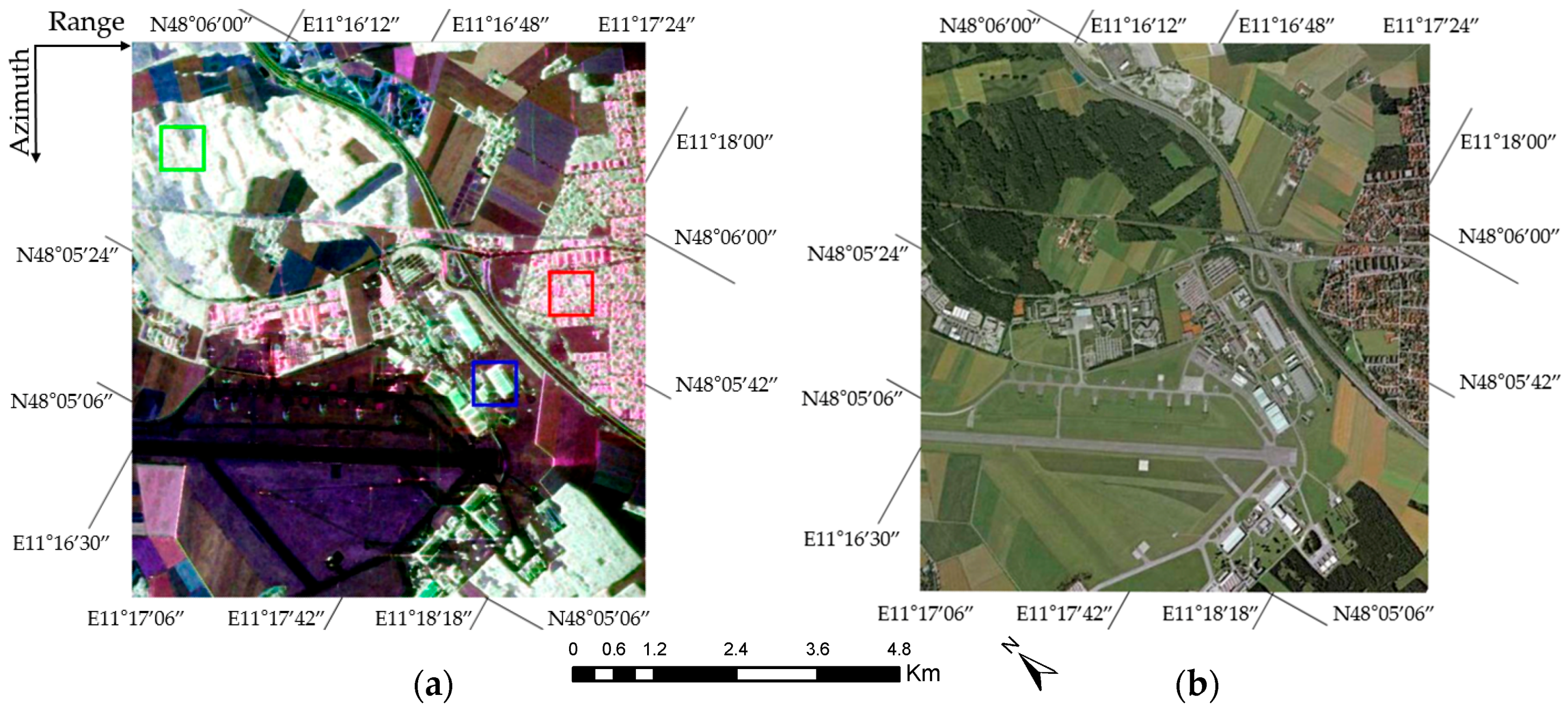
If the flat wall of a building is parallel to the flight direction of the SAR sensor, the building has an azimuth orientation angle (AOA) of 0°. The AOA is off 0° once both are not parallel. The range of the AOA is between −45° (−π/4) and 45° (−π/4). The shape of a building or street pattern is usually rectangular. One needs only to consider the AOA from –45° to 0° or from 0° to 45°. The AOA range between 0° and 45° is used in this study. Scattering characteristics of urban targets are greatly affected by their AOAs in addition to physical dimension, shape, spatial density, and pattern (e.g., [1,2,3,4,5]). Figure 1a is a Pauli Red, Green, and Blue (PauliRGB) image of the German Aerospace Center (DLR) E-SAR L-band PolSAR data near Oberpfaffenhofen, Germany (https://earth.esa.int/web/polsarpro/data-sources/sample-datasets). The image size is 1300 rows by 1200 columns, covering an area about 2.50 km wide by 2.53 km high. The widely-accepted interpretation of the PauliRGB image is that houses, buildings, and infrastructure in urban areas primarily act as dihedral corner reflectors, and are represented in red. The vegetated area has strong volumetric scattering, and is shown green. The blue color represents a target with strong surface scattering. With the reference of the optical image from GoogleEarth® (Version: 7.1.8.3036 (32-bit), Google, 1600 Amphitheatre Parkway, Mountain View, CA, USA, Figure 1b), the interpretation is correct for the urban area, which is highlighted in a red square, and for vegetated surfaces, as outlined by a green square. However, buildings are clearly inside the area highlighted by the blue square, but they are considered to be vegetation (Figure 1a). The misinterpretation is caused by the AOAs of buildings that are significantly un-parallel with the flight direction.
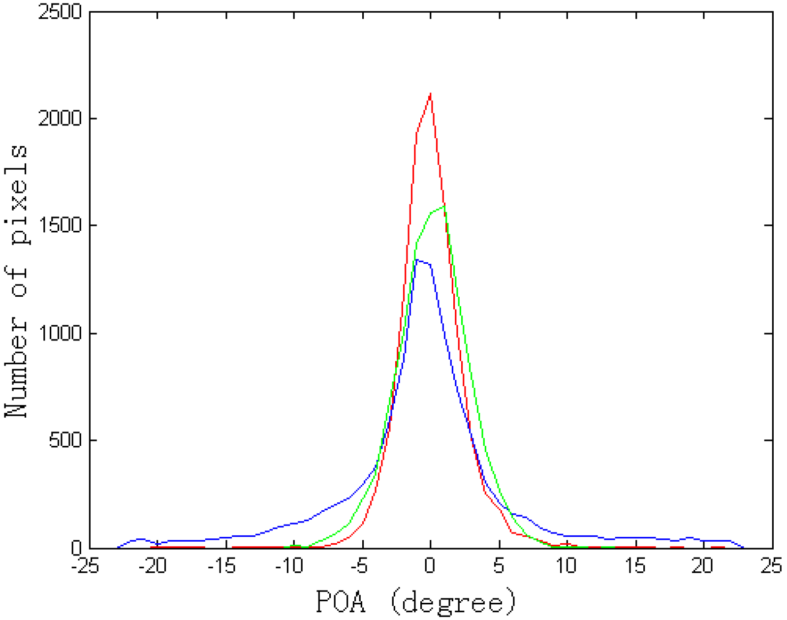
Unless the shape of a building is cylindrical, a tree is typically more azimuthally symmetrical than the building is. Thus, the tree is generally less azimuthally dependent in comparison with the building. Values of polarization orientation angles (POAs) widely used in the de-orientation of the AOAs should be smaller in forested areas than in urban areas [1,2,3,4,5]. Histograms of POAs extracted from the red, green, and blue squares in Figure 1a are shown in Figure 2. Each square consists of 100 × 100 pixels. Pixels within the red square represent urban areas with small AOAs, pixels within the green square represent forested areas, and pixels within the blue square denotes urban areas with large AOAs. The color of the histogram curve is related to the color of the square in the figure. The angles vary from −22.5° (−π/8) to 22.5° (π/8) with the majority of them near 0° (0). The AOA curves from three squares are overlapped heavily. The algorithms coupled with the de-orientation of the POA approach [2,3,4,5] cannot effectively characterize urban targets that have a wide range of AOAs.
The decomposition of PolSAR data has played a significant role in the understanding and identification of ground targets, and a number of volumetric scattering models have been proposed [5,6,7,8,9,10,11,12,13,14,15,16,17,18]. For example, eigenvalues and eigenvectors of the covariance matrix of PolSAR data were used to derive the volumetric scattering components [6,7]. Freeman and Durden [8] decomposed the PolSAR data into components of surface scattering, double-bounced scattering, and volumetric scattering. Although the Freeman and Durden decomposition algorithm [8] could be generally applied to forested areas with variable compositions of tree species, there was concern over whether reliable geophysical parameters in forested areas could be extracted from PolSAR data. Thus, Freeman [9] simplified the Freeman and Durden decomposition algorithm [8] into two major components with volumetric scattering from canopy layer and double-bounced trunk ground interactions, or with volumetric scattering from canopy layer and ground surface scattering.
Since randomly oriented long-thin cylinders or dipoles were used to model the volumetric scattering [8], the volumetric scattering could be overestimated. To reduce the overestimation, Yamaguchi et al. [5,10] used a randomly oriented dipole model, a vertically orientated dipole model, or a horizontally orientated dipole model to model the volumetric scattering. The latter two models produced less volumetric scattering as compared to that of the randomly oriented dipole model. Furthermore, Yamaguchi et al. [5,10] extracted a helix scattering component from their volumetric scattering component. An et al. [11] developed a new volumetric scattering model to characterize the total randomness that is the main feature of volumetric scattering. To model a broad range of canopies in forested environments properly, researchers alternatively proposed a suite of generalized volumetric scattering models [12,13,14]. In summary, algorithms [5,6,7,8,9,10,11,12,13,14] are mainly developed for the understanding of the polarimetric scattering mechanisms in forested environments. However, the algorithms might become ineffective in the identification of an urban target whose AOA is largely off 0° vs. a non-urban target. When the AOA of an urban target is near 45°, its backscattering is cross-scattering that usually comes from the volumetric scattering of tree canopies (e.g., Figure 1a). Thus, if these algorithms are directly used, the urban target is very likely be classified into the vegetation category due to the ambiguity in scattering mechanisms.
To reduce ambiguity and to avoid the misclassification eventually, Chen et al. [15] proposed an algorithm to suppress the overestimation of the volumetric scattering in urban areas, but the success of their algorithm was limited. Hong and Wdowinski [16] added a scattering model for a rotated dihedral plane to correctly describe the cross-scattering from a rotated dihedral corner reflector (CR) and proposed a four-component decomposition algorithm. Xiang et al. [17] used a generalized scattering model to characterize scattering mechanisms of buildings with different POAs and proposed a five-component decomposition algorithm. Xie et al. [18] implemented the generalized volumetric scattering model [13] and the simplified adaptive volume scattering model [14] into the decomposition algorithm. Satisfactory results were obtained. However, since the non-linear least squared optimization method was used to invert the model parameters simultaneously [18], the inversion process was quite time-consuming.
The combination of the decomposition and classification is then explored (e.g., [19,20,21]). Azmedroub et al. [21] decomposed the PolSAR image using Yamaguchi et al. (2011) [5], the Yamaguchi-2011 algorithm for short first. The Wishart classification was next applied to obtain the final delineation of urban targets. As pointed out by Du and Wang [1], the Yamaguchi-2011 algorithm misclassified houses and buildings into the vegetation category. This misclassification was the unavoidable source of error in Azmedroub et al. algorithm. Zou et al. [22] proposed an eigenvalue and eigenvector based four-component decomposition algorithm. They linked the eigen-decomposition algorithm and the model-based decomposition algorithm through a lookup table. As a result, the misclassification in urban areas decreased. However, the level of the classification accuracy could be still improved.
Although a coherence coefficient algorithm (e.g., [1,23]) can theoretically resolve the misclassification entirely, one needs at least two PolSAR images to obtain one coherence image. Thus, the algorithm is not usable when there is only a single PolSAR image, or if the coherence image cannot be derived, although multiple PolSAR images may exist. Therefore, the objectives of this study are to further resolve the ambiguity in scattering mechanisms from urban and non-urban targets, and to develop an algorithm that will improve the performance of an existing and widely-used model-based decomposition algorithm. The algorithm will be applicable to land cover types including urban areas, and upland and flooded forest stands. In addition, the proposed algorithm must be not only valid, but also simple in implementation and computationally efficient. In particular, a correlation coefficient revealing the distinct characteristics of urban and non-urban targets is introduced. Then, the coefficient is used to modify the volumetric scattering model component of Yamaguchi et al. (2005) [10] or the Yamaguchi-2005 algorithm for short. Before details of our algorithm development are given, models/algorithms reviewed above are categorized on the bases of the decomposition approach, primary usage, and secondary usage (Table 1). With the table, a reader might achieve a better understanding of studies of the PolSAR decomposition in forested and urban areas.
2. Methodology
2.1. Coherency Matrix [T] and Correlation Coefficient r
A 3 × 3 coherency matrix, [T] describing scattering mechanisms of ground targets is defined as
where Spq (p = H or V, and q = H or V) is the element of a scattering matrix at polarization pq. In the PauliRGB decomposition, element T11 stands for the surface scattering energy, T22 the double-bounced scattering energy, and T33 the volumetric scattering energy. In a PolSAR image, numerous scatterers exist within an image pixel, and can produce all three types of scattering energy. Thus, scattering characteristics inside one pixel may not be well described when each matrix element is individually used. The combined use of the elements is considered.
When the AOA of an urban target (e.g., a building) is near-zero or small, there is strong double-bounced scattering return. The value of T22 is high, but the value of T33 is low. When the AOA is large especially ~45°, there is strong volumetric scattering. T33 is high but T22 is low. Thus, the combination of T22 and T33 properly characterizes scattering mechanisms of urban targets regardless of their AOAs. The correlation coefficient is defined as:
The rationale to introduce r includes (i) T22, in the PauliRGB image is a widely-used parameter to represent urban targets with strong double-bounced scattering, (ii) T33 is related to the volumetric scattering that can come from tree canopies in forested areas, and from buildings/houses and infrastructure having large AOAs, (iii) the increase of double-bounced scattering from the urban targets, and the reduction of the volumetric scattering from the same urban targets can be well assessed by changes of T22 and T33 values, and (iv) r is simple to compute in comparison with [2,3,4,5,18]. The computational efficiency of the algorithm should be high as shown later.
2.2. The Addition of a Volumetric Model for Urban Targets with Large AOAs and the Proposed Algorithm
When the PolSAR image is decomposed using a 3 × 3 coherency matrix, [T], the volumetric scattering model is in the form of a diagonal matrix (e.g., [11,17]) or:
As the proposed algorithm is a revision of the Yamaguchi-2005 algorithm (Table 1) by modifying the volumetric scattering component using r, there are no changes of the surface scattering, double-bounced scattering, and helix scattering components of the Yamaguchi-2005 algorithm. Thus, the proposed algorithm is expressed as:
With the reference to Equations (1)–(4) and the Yamaguchi-2005 algorithm, A, B, and C are solved next. First:
where Im(·) is an operator to extract the imaginary part of a complex value. Then:
If (Re(SHHSVV*) ≥ 0), then . Re(·) is an operator to extract the real part of a complex number. Thus:
and
If (Re(SHHSVV*) < 0), then . Therefore:
and
Scattering powers contributed from the surface scattering (Ps), double-bounced scattering (Pd), volumetric scattering (Pv), and helix scattering (Pc) are:
The Yamaguchi-2005 algorithm works satisfactorily in the decomposition/classification of the surface, urban targets with 0° or small AOAs, and forested areas. However, when the algorithm is used to decompose targets of houses/buildings and street patterns with large AOAs in urban areas, the strong volumetric scattering from the targets are obtained, as shown later in this study. If the decomposed result is showed as a PauliRGB image, the targets are presented in green or green-dominated colors. Thus, the urban targets are unfortunately considered as vegetation. The improper modeling of the urban targets with the current three volumetric models in the Yamaguchi-2005 algorithm can be attributed for the cause. The revision of the volumetric scattering models is in order. Mathematically, the revised volumetric scattering model can be written as:
Following criteria are employed to determine the use of which Model in (12).
- (i)
- Previous studies in the PolSAR data analysis and canopy backscattering modeling (e.g., [24,25,26]) suggest that |SHH|2 is usually greater than |SVV|2 in flooded forests or coniferous forest stands where strong double-bounced scattering caused by trunk-ground interactions exists. This relationship is especially true when the radar wavelength is long such as with an L-band sensor [24,25,26]. Thus, to make this mitigation and proposed algorithm applicable to PolSAR data when acquired at a long radar wavelength, and from areas consisting of urban targets, flooded forests, and coniferous forest stands, we compare |SHH|2 and |SVV|2. If |SHH|2 > |SVV|2, then [T]vol_Yamaguchi-2005 is used.
- (ii)
- The Yamaguchi-2005 algorithm can effectively decompose/classify the surface, urban targets with 0° or small AOAs, and forested areas. Thus, if the double-bounced scattering or surface scattering of an image pixel is more than 50%, then [T]vol_Yamaguchi-2005 is employed.
- (iii)
- Otherwise, [T]vol_4th is used.
Next, the derivation of [T]vol_4th based on r is detailed. If the PolSAR image is expressed in [T], the volumetric scattering component in the Freeman-Durden decomposition [8] is:
Hong and Wdowinski [16] model the volumetric scattering from an oriented building as:
To be similar to Equation (14), one can rewrite Equation (15) as:
where . However, θdom itself or a function of θdom such as cannot well characterize urban targets with large AOAs as shown in Figure 2. Alternatively, r or f(r) is introduced. In other words, we use f(r) to replace f(θdom) in Equation (16), and hybrid Equations (13) and (16) to revise the volumetric scattering model as:
When f(r) ≠ 0, [T]vol_4th, Model (17a) is the combination of the volumetric scattering model of Freeman and Durden [8], and modified volumetric scattering model for oriented buildings [17]. If f(r) = 0, [T]vol_4th, Model (17b) becomes an identity matrix multiplied by a factor of two and it produces the strongest volumetric scattering [11]. It should be noted that (proportion to) is used to simplify above discussions. However, solutions of model parameters are bounded by Equation (4).
According to Equation (6), the volumetric scattering is proportion to 1/C. The larger the C value is, the smaller the volumetric scattering. Also, with regard to Equations (8) and (9), the double-bounced scattering is negatively related to B. If the value of B is small or even negative, the double-bounced scattering increases. Thus, to group urban targets regardless of their AOAs into an urban category properly, one should set C to be as large as possible, and B to be small in Model (17c). Possible solutions can be countless as long as f(r) is positive and increases. Thus, to make the revised model simple and effective, we select f(r) = 3r, and Model (17c) becomes:
Finally, to ensure that C is large, B is small for a range of r, further operations are considered. If r is higher than a threshold value such as 0.01 (as shown in Section 3.1), and less than 2/3, the reciprocal, 1/r is used. If r is ≤ 0.01 or ≥ 2/3, there is no change of r. In addition, even though there are other methods to increase r, but the reciprocal function is simple, and is chosen. For example, if one wants to increase r = 0.1 to r = 10, the reciprocal function works well even though one can multiply r by 100. If one wants to change r = 0.02 to r = 50, the reciprocal function works as well. However, one must multiply r by 2500 to achieve that. Thus, there would be multiple factors to consider if the multiplication function were used. As A, B, and C are solved on a pixel-by-pixel basis, the volumetric scattering model is self-adaptive. Figure 3 is the summary of the proposed model-based decomposition algorithm.
3. Results and Discussion
3.1. Correlation Coefficient r
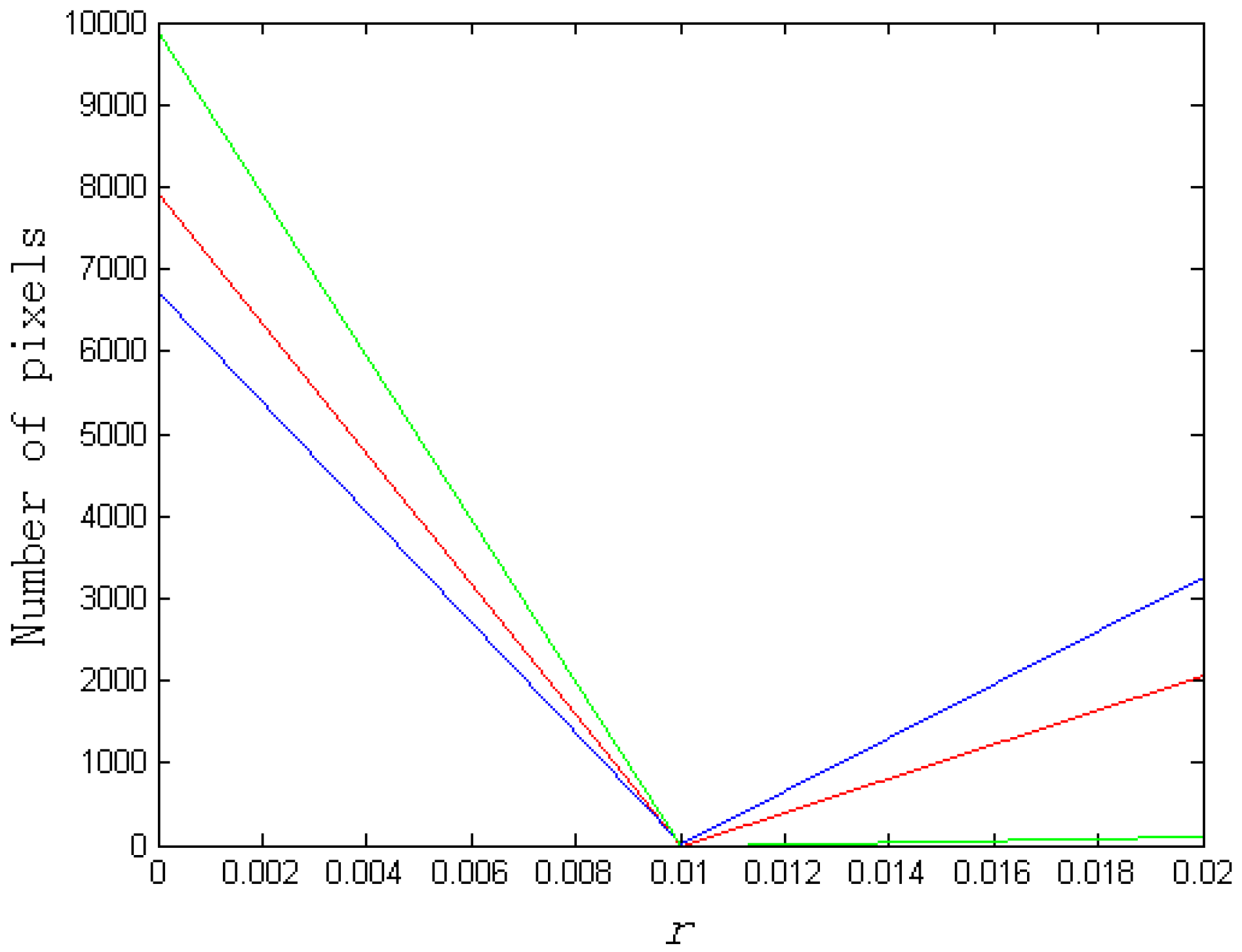
r values were studied using the Oberpfaffenhofen data. Overall, r values were low in forested areas and in open surface areas, but ranged from moderate to high in urban areas with variable AOAs. Then, r values were extracted from pixels within three squares (Figure 1a) and quantified. Histograms were shown in Figure 4. r was low in the forested areas (the green line). r values (the red and blue lines) in urban areas varied from low to high, regardless whether AOAs were small or large. The difference of r values between urban targets and forested (or non-urban) areas should help distinguish both from each other. In addition, the three lines crossed each other near 0.01, which is the threshold used in the algorithm. It should be noted that the maximum value of r in the histogram was set to 0.02 for the purpose to show small r values, although r would be larger than 0.02. The effectiveness of r in the delineation of urban targets was next investigated.
3.2. Validation of the Algorithm Using Goldstone Polarimetric Data
The algorithm is applied to the National Aeronautics and Space Administration/Jet Propulsion Laboratory (NASA/JPL) Airborne Synthetic Aperture Radar (AIRSAR) C-band PolSAR data collected at Goldstone, California, USA [6,27]. Numerous trihedral CRs, and dihedral CRs with AOAs of 0° and 45° have been deployed on the flat and dry lake bed for the calibration of the AIRSAR sensor. A trihedral CR produces the strongest surface scattering. The strongest double-bounced scattering is generated when a dihedral CR is with an AOA of 0°. In this study, the dihedral CRs could stand for houses/buildings and street patterns with a 0° AOA in urban areas. A dihedral CR with an AOA of 45° outputs the strongest volumetric backscattering that could represent the volumetric backscattering from urban targets with AOAs of 45°. However, from the classification point of view, dihedral CRs, regardless of their AOAs should be grouped into the dihedral CR category. Analogously, regardless of the AOAs of houses, buildings, and street patterns having in urban areas, they should be classified into the urban category.
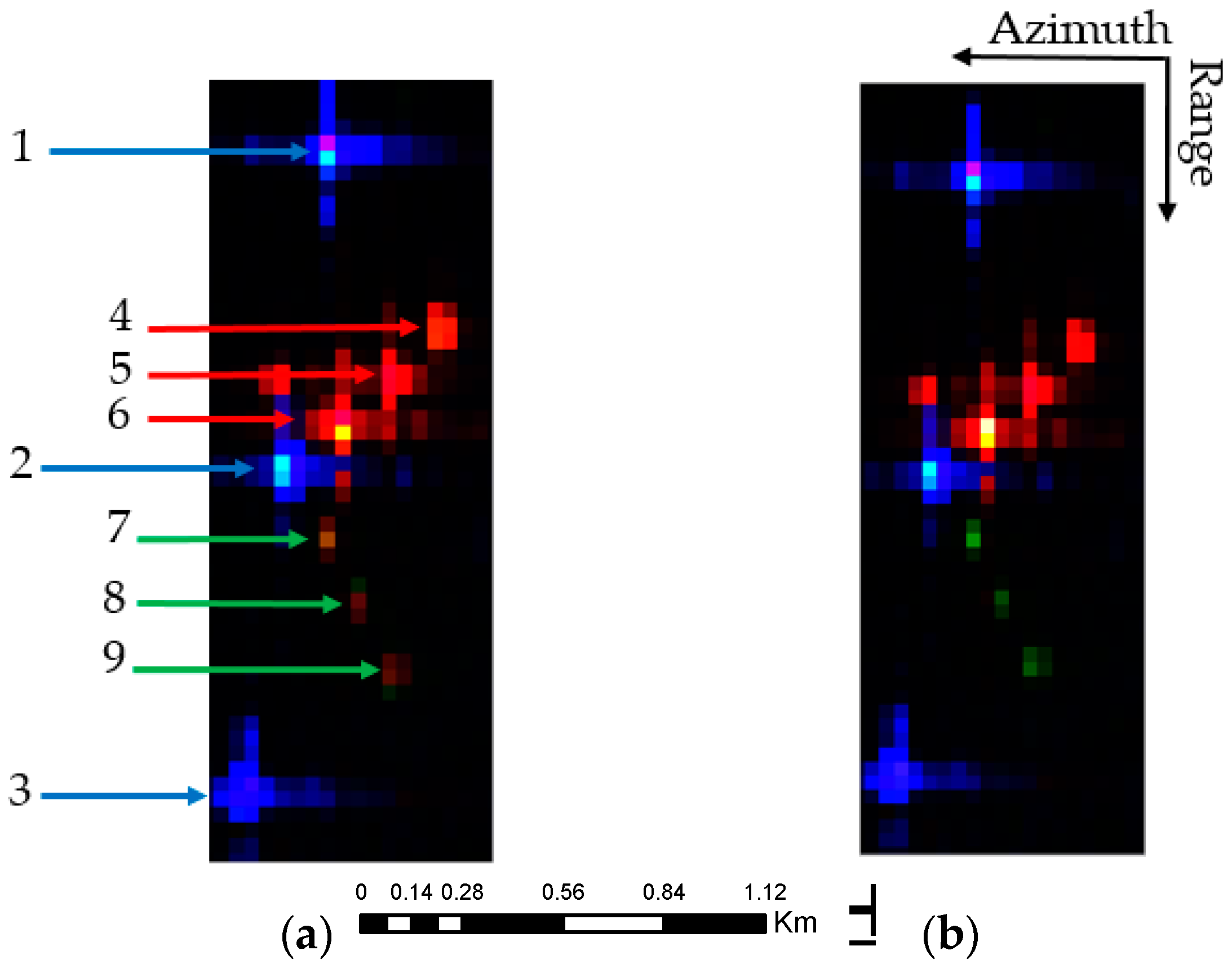
A PauliRGB image was then obtained after the algorithm. A sub-image consisting of three trihedral CRs (numbered as 1–3), three dihedral CRs with AOAs of 0° (4–6), and three dihedral CRs with AOAs of 45° (7–9) was extracted and shown (Figure 5a). The image was 550 rows by 200 columns. Since sizes of the trihedral CRs were much larger than those of the dihedral CRs [27], the backscatter from the trihedral CRs was much stronger than that from the dihedral CRs. The trihedral CRs producing the strongest surface scattering were displayed in blue color. The dihedral CRs (4, 5, and 6) with AOAs of 0° created strong double-bounced scattering. They were displayed in red. Dihedral CRs 7–9 with AOAs of 45° were shown in orange-magenta, that is, a mixture of red and green colors with the red component being dominant. Since the AOAs of dihedral CRs 7–9 were 45°, the CRs ought to produce strong volumetric backscattering. Thus, the algorithm suppressed the volumetric scattering but elevated the double-bounced scattering. The scattering mechanisms from dihedral CRs 4–6 and CRs 7–9 then similar. If dihedral CRs 4–6 were to mimic urban targets with 0° or small AOAs, and dihedral CRs 7–9 were to model urban targets with large AOAs (up to 45°), both types of mimicked urban targets should be identified as “urban targets”.
To quantify the effectiveness of the proposed algorithm, we computed the percentage of power of Ps, Pd, and Pv in the sum, (Ps + Pd + Pv) for CRs 1–9 (Table 2) [Pc in (11) is not related to r, A, B, or C. Thus, the sum consists of only three components.] The percentage was tabulated in each cell of the first row, and was denoted in bold font. The surface scattering dominated for trihedral CRs (1–3) because the percentage was 98.1% or higher. The percentage of the double-bounced scattering was 96.1% or higher for dihedral CRs 4–6 with AOAs of 0°. For dihedral CRs (7–9) with AOAs of 45°, double-bounced scattering was at least 53.6%, whereas the volumetric scattering was 41.9% or less. Thus, the increase of double-bounced scattering and decrease of volumetric scattering was evident.
In comparison, the Yamaguchi-2011 algorithm was applied to the Goldstone AIRSAR data. The Yamaguchi-2011 algorithm revised from the Yamaguchi-2005 algorithm was designated to resolve the AOA problem in the identification of urban targets. Figure 5b is the result, shown as a PauliRGB image. Trihedral CRs 1–3 are displayed in blue, showing strong surface scattering. The percentage is 98.1% or larger, and is shown in Roman font (Table 2). Dihedral CRs 4–6 are shown in red, indicating strong double-bounced scattering. The percentage is 98.0% or higher (Table 2). Dihedral CRs 7–9 are displayed in green, representing strong volumetric scattering. The percentage is at least 82.6% or greater (Table 2). Therefore, if dihedral CRs 7–9 were to model urban targets with large AOAs, the targets would have strong volumetric scattering and would be classified into the vegetation category under the PauliRGB classification scheme. For the final comparison, the difference of two percentages (i.e., the percentage in the first row minus that in the second row) is given cell-by-cell (Table 2). Both algorithms were very similar in the decomposition of the scattering mechanisms from the trihedral CRs, and dihedral CRs with AOAs of 0°, because the difference in absolute value is 3.5% or less. However, for dihedral CRs 7–9, the percentage of double-bounced scattering increased by at least 49.9% and the percentage of volume scattering decreased by more than 56.2%. Therefore, the proposed algorithm had little effect on the decomposition of trihedral CRs and dihedral CRs with AOAs of 0°. The algorithm could decrease the volume scattering, but increased the double-bounced scattering for dihedral CRs with AOAs of 45°.
3.3. Decomposition of Oberpfaffenhofen Polarimetric Data
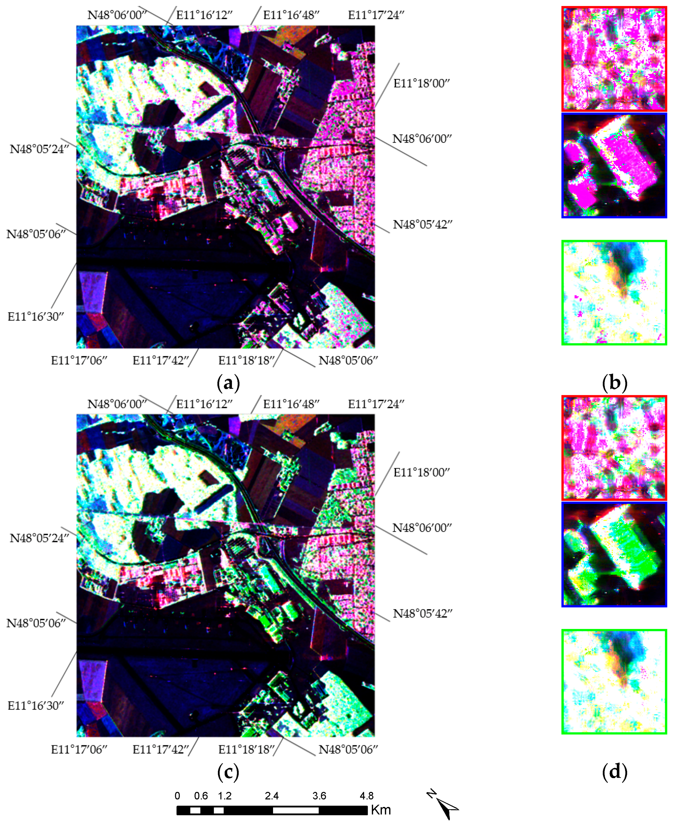
The proposed algorithm was applied to the Oberpfaffenhofen E-SAR data. The decomposition result was shown as a PauliRGB image (Figure 6a). Almost all urban areas with variable AOAs (as shown in Figure 1b) were displayed in red or magenta colors (Figure 6a). The percentage of double-bounced scattering was dominant among the surface scattering, double-bounced scattering, and volumetric scattering mechanisms. Figure 6b was the enlarged views of the red, green, and blue squares (as identified in Figure 1a). Urban targets in red and blue squares (the top two) were effectively identified because pixels with red and magenta colors dominated the image. Pixels inside the green square were mainly presented in green, cyan, and white colors. Then, averaged percentages of three types of scattering mechanism for each square were calculated (Table 3). Inside the red square, the percentages of the surface scattering, double-bounced scattering, and volumetric scattering were 32.2%, 59.0%, and 8.8%, respectively. Double-bounced scattering was dominant. In the green square, the volumetric scattering was 45.7%. The surface scattering was 27.2% and the double-bounced scattering 27.1%. The volumetric scattering was the largest one. Within the blue square, the surface scattering, the double-bounced scattering, and volumetric scattering were 37.9%, 44.7%, and 17.4%, respectively. The percentage of the double-bounced scattering was the largest.
The Yamaguchi-2011 algorithm was also applied to the Oberpfaffenhofen E-SAR data. Results were shown in Figure 6c. The enlarged views of three selected squares were provided (Figure 6d). In comparison, the number of pixels with red and magenta colors in Figure 6a was much greater than that of Figure 6c. The increase in the number of pixels with red and magenta colors was clear, as shown in the enlarged views of the red and blue squares (Figure 6b c.f. Figure 6d). Thus, the proposed algorithm visually outperformed the Yamaguchi-2011 algorithm.
Averaged percentages from surface scattering, double-bounced scattering, and volumetric scattering extracted from three squares (Figure 6d) were tabulated (Table 3). Inside the red square, the averaged percentage of the double-bounced scattering was 57.7% using the Yamaguchi-2011 algorithm. The double-bounced scattering was dominant among three types of scattering mechanism as derived from both algorithms. The differences between the percentages of the surface scattering, double-bounced scattering, and volumetric scattering were small. For the vegetated areas (outlined by the green square), the averaged percentage of volumetric scattering was 46.2% from the Yamaguchi-2011 algorithm, and 45.7% from our algorithm. Volumetric scattering was dominant. Therefore, both algorithms performed similarly.
Within the blue square, the Yamaguchi-2011 algorithm produced 25.7% of the surface scattering, 31.3% of the double-bounced scattering, and 43.0% of the volumetric scattering (Table 3). In comparison, the proposed algorithm increased the double-bounced scattering by 13.4%, but reduced the volumetric scattering by 25.6%. Thus, the chance for misclassification decreased if our decomposed results were next used to delineate urban and non-urban targets using the PauliRGB classification scheme.
It should be noted that the same PolSAR data were studied, and the decomposition results have been published (Figure 5d,e, p. 1292, [22]). Overall, previous results and ours results regarding vegetated areas and open surfaces were comparable. However, in urban areas such as the areas near the middle and right side of the figure, there were significantly more red/magenta pixels in Figure 6a than Figure 5d or Figure 5e, in [22]. Thus, the proposed algorithm reduced the volumetric scattering but elevated double-bounced scattering further. This was especially true for the area outlined by the blue square in (our) Figure 1a. That area was dominated by buildings with AOAs near 45°. The additional reduction of the volumetric scattering energy but the increase of double-bounced scattering energy should improve the level of classification accuracy.
3.4. Applicability of the Algorithm to Two Additional PolSAR Datasets
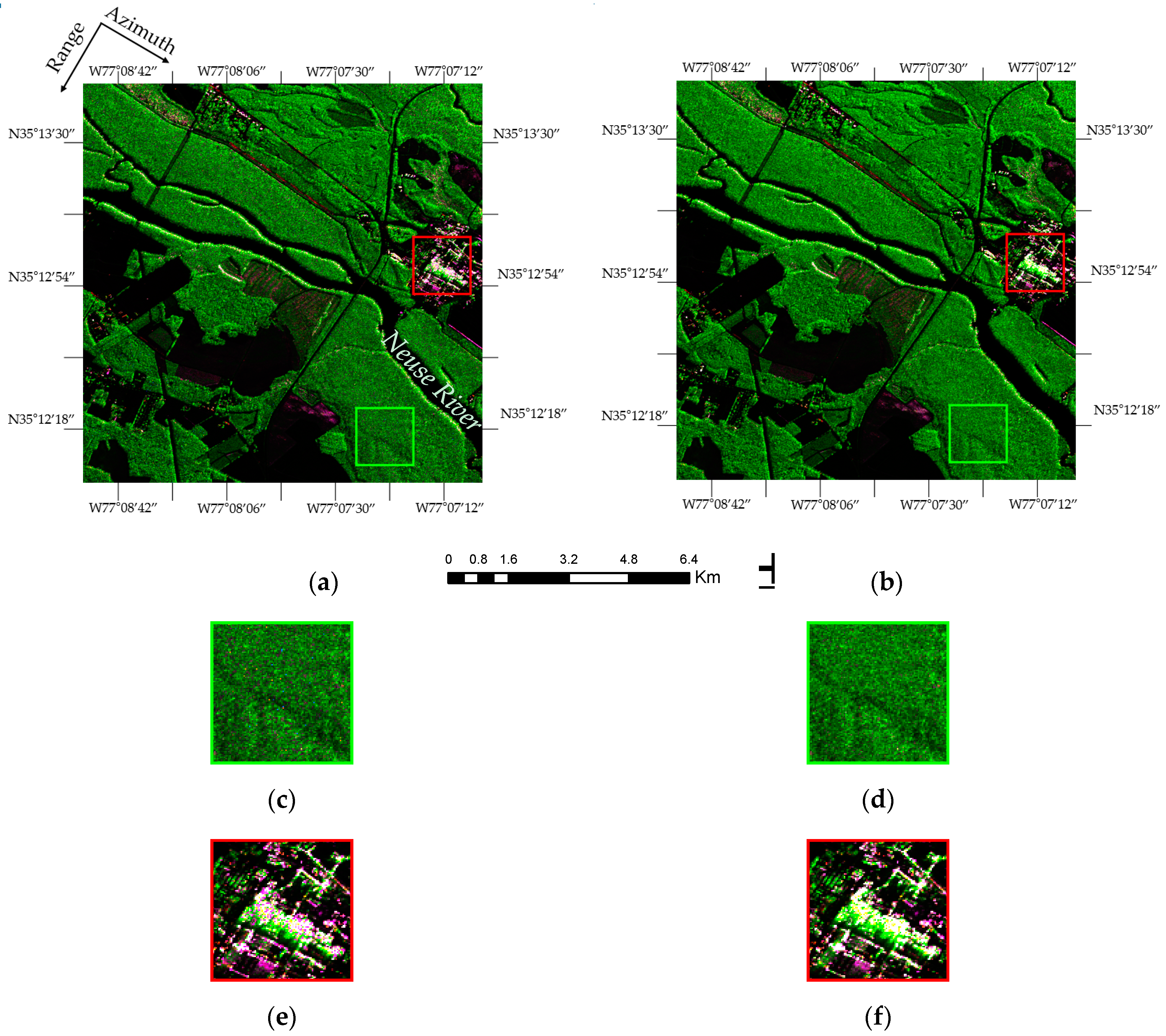
The first dataset tested was the NASA/JPL Uninhabited Aerial Vehicle Synthetic Aperture Radar (UAVSAR) L-band PolSAR dataset (UA_Ingley_31201_09059_003_090813_L090_CX_01) acquired on 13 August 2009. The study area (Figure 7a) is about 7km south of Vanceboro, North Carolina, USA. The image is 700 rows × 700 columns covering an area about 3.60 km in the longitude direction and 4.20 km in the latitude direction. The major reason for using this area is that the dominant landuse and land cover type is vegetation with mature loblolly pine (Pinus taeda) in upland forest stands, and large cypress (Taxodium distichum) trees in flooded forest stands. A mature loblolly pine is typically nearly 20–30 m tall and has a small tree crown. Its trunk is 20–40 cm in diameter at breast height (DBH). The number of trees per ha. or stand density ranges from several hundred up to 1000. The cypress trees in the flooded forest stands are mainly situated along the banks of the Neuse River and its tributaries, in North Carolina. Mature cypress trees are tall (>30 m) and large in DBH (>80 cm). Stand density is in tens to hundreds of trees per ha. Tree crown can be fully developed if the stand density is low, or a cypress tree is near the stand edges. Thus, the double-bounced scattering from the trunk-ground interactions at L-band should be strong from the upland forest stands of pines, and from flooded forest stands of cypresses. The decomposed results using the proposed algorithm and the Yamaguchi-2011 algorithm are shown in Figure 7a and Figure 7b, respectively. In the vegetated areas, both figures were very similar overall. The close-up views from a forested area further indicated the similarity (Figure 7c c.f. Figure 7d). Thus, the proposed algorithm is applicable in the forested areas with the dry or flooded ground surface conditions.
It should be noted that the proposed algorithm delineated more urban targets as shown in red and magenta colors in Figure 7e when compared to the delineation using the Yamaguchi-2011 algorithm (Figure 7f). Figure 7e or Figure 7f depicts the facility for paper manufacturing by Weyerhaeuser Corporation, USA. The facility consists of buildings and man-made structures with a wide range of AOAs.
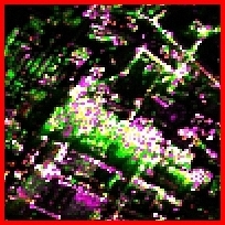
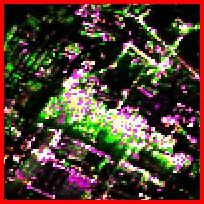
The second one was the Japan Advanced Land Observing Satellite/Phased Array type L-band Synthetic Aperture Radar (ALOS/PALSAR) dataset (ALPSRP202350750) near San Francisco, California, USA. The data were acquired on 11 November 2009. A subimage with 1000 rows by 1000 columns covering the area about 12.6 km wide by 12.7 km high was extracted. Decomposed results using the proposed and Yamaguchi-2011 algorithms are shown in Figure 8a and Figure 8b, respectively. Both figures were potentially visually similar. With the reference to hi-resolution optical image, the majority of the urban areas in San Francisco were correctly identified. However, the area near the San Francisco side of the Oakland Bay Bridge as highlighted in the red square (Figure 8a or Figure 8b), was comprised of buildings, street patterns, and infrastructure with a wide range of AOAs. The area was 90 × 90 pixels. The corresponding enlarged views were shown in Figure 8c,d. Both algorithms may not produce satisfactory outcomes because green color overall dominated. However, there were more red/magenta spots in Figure 8c than in Figure 8d. The proposed algorithm increased the double-bounced scattering, but decreased the volumetric scattering to some extent. Changes in the relative importance of the surface scattering, double-bounced scattering, and volumetric scattering were quantified next.
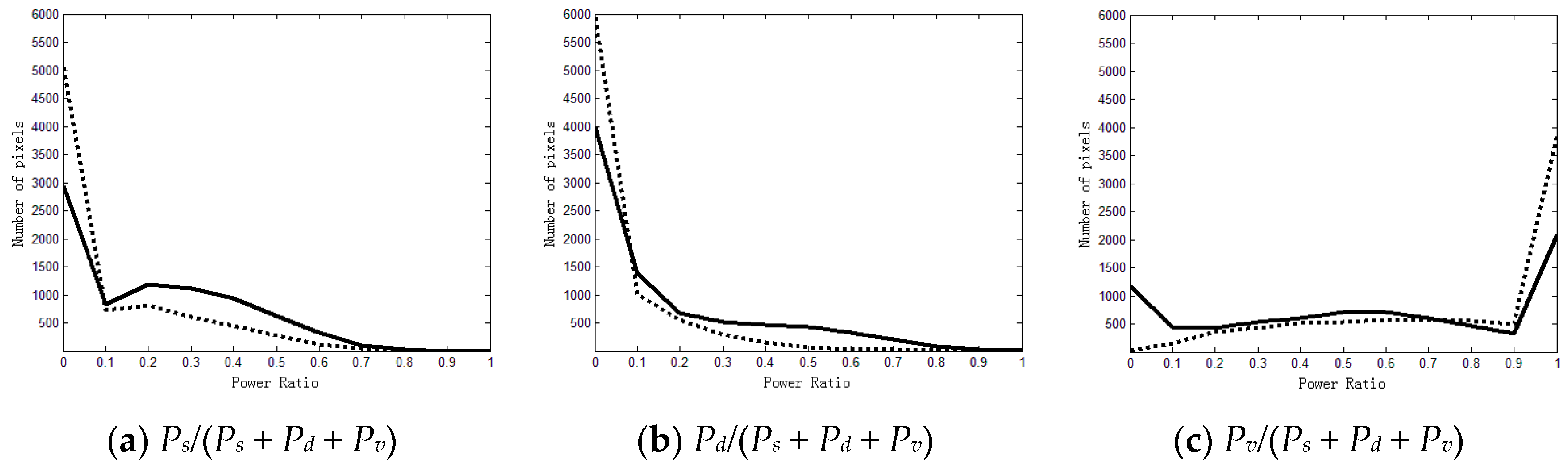
Histograms of Ps/(Ps + Pd + Pv), Pd/(Ps + Pd + Pv) and Pv/(Ps + Pd + Pv) are shown in Figure 9. In the figure, the solid line stands for the frequency counts derived from the proposed algorithm and the dotted line from Yamaguchi-2011 algorithm. In Figure 9a, both algorithms performed similarly overall even though the number of pixels with large Ps values derived by the proposed algorithm may increase. In Figure 9b, the histogram of the double-bounced scattering using the proposed algorithm was spread out between 0 and 1. The histogram derived from the Yamaguchi-2011 algorithm could be clustered near the low-end with the majority of pixels having Pd ≤ 0.1 (80.8% of the total number of pixels). Thus, among three types of scattering mechanism, the increase of the relative importance of Pd after the proposed algorithm was clear. After the proposed algorithm, the majority of pixels had a small value of Pv (Figure 9c). In comparison, most pixels had relative large Pv values when the Yamaguchi-2011 algorithm was employed.
3.5. Computational Efficiency
The proposed algorithm, the Yamaguchi-2011 algorithm, and the Xie et al. algorithm [18] were applied to four UAVSAR datasets. The image sizes were 200 × 200, 400 × 400, 800 × 800, and 1600 × 1600 pixels, respectively. The central processing unit (CPU) used was an Intel CoreTM I5-4590 at 3.30 GHz, with a memory of 8 GB. Windows 7 64-bit with Service Pack-1 was the operating system used. MATLAB R2013b 64-bit was the software environment used to process PolSAR datasets. The processing time was recorded (Table 4). As the image size increased, the processing time was almost linearly increased using the proposed algorithm. However, for Yamaguchi-2011 and Xie et al. algorithms, the processing time could be increased geometrically. Overall, the proposed algorithm was the most efficient.
4. Conclusions
In model-based PolSAR decomposition algorithms, urban targets are usually delineated based on the existence of strong double-bounced scattering. However, buildings and street patterns with large azimuth orientation angles (AOAs) can produce strong volumetric scattering that is typically considered as a scattering characteristic from vegetated surfaces. Thus, the misclassification of urban targets as vegetation category occurs if the PauliRGB classification scheme is considered. To mitigate the misclassification, we introduced a correlation coefficient to characterize scattering mechanisms of urban targets of variable AOAs. Then, the coefficient was used to modify the existing volumetric scattering model. A revised decomposition algorithm was developed.
The validity and effectiveness of the algorithm was examined using NASA/JPL AIRSAR C-band PolSAR data of Goldstone, CA, USA. Within the AIRSAR data, there were dihedral CRs with AOAs of 0°, and dihedral CRs with AOAs of 45°. After the algorithm, dihedral CRs with the AOAs of 0° and 45° created strong double-bounced scattering. Since a dihedral CR with a 45° AOA generates strong volumetric backscattering, the algorithm successfully suppresses the volumetric scattering but elevates the double-bounced scattering. Thus, if dihedral CRs with AOAs of 0° are to mimic urban targets with 0° or small AOAs, and dihedral CRs with AOAs of 45°, to model urban targets with large AOAs, both types of mimicked urban targets should be identified as “urban targets”. Then, the algorithm was applied to DLR E-SAR L-band PolSAR data near Oberpfaffenhofen, Germany, NASA/JPL L-band UAVSAR PolSAR data near Vanceboro, NC, USA, and Japan ALOS/PALSAR PolSAR data of San Francisco, CA, USA. The algorithm improved on the level of accuracy in the delineation of urban targets versus non-urban targets. In addition, the algorithm had little effect on the surface or volumetric scattering characteristics from ground targets in urban areas, and in forested areas with dry or inundated ground surface condition, and on the double-bounced scattering from mature loblolly pine stands and flooded cypress stands. Therefore, the objectives of this study were met because the ambiguity in scattering mechanisms from urban and non-urban targets were further resolved. An algorithm applicable to a range of land cover types including urban areas, and upland and flooded forest stands was thus developed. The algorithm not only improved on the performance of existing and widely-used model-based decomposition algorithms, but also was simple and efficient.
Finally, as shown in Figure 8a, the algorithm could not suppress volumetric scattering enough or significantly, and was also unable to elevate the double-bounced scattering sufficiently. Further investigation is needed to improve the performance of the algorithm in this regard.
Supplementary Materials
Supplementary File 1Acknowledgments
This work was sponsored by the National Natural Science Foundation of China under grants 41471361 to the University of Electronic Science and Technology of China (UESTC), and the Fundamental Research Funds for the Central Universities under grant ZYGX2013Z006 of UESTC. The Goldstone data were obtained from NASA/JPL, USA. The Oberpfaffenhofen data were downloaded from https://earth.esa.int/web/polsarpro/data-sources/sample-datasets. The Vanceboro and San Francisco data were obtained from the Distributed Active Archive Center (DAAC) at the Alaska Satellite Facility (ASF), USA. We thanked Qinghua Xie who graciously provided his computer codes for their algorithm to us. The time and effort of anonymous reviewers were greatly appreciated.
Author Contributions
Wang and Duan conceived the study. Duan designed the experiment, and analyzed PolSAR datasets in consultation with Wang. Duan and Wang wrote the paper.
Conflicts of Interest
The authors declare no conflicts of interest.
References
- Du, A.; Wang, Y. Compensation for Azimuth Angle or Scale Effect on Building Extraction in Urban Using SAR Scales of Polarization and Coherence. IEEE J. Sel. Top. Appl. Earth Obs. Remote Sens. 2016, 9, 2601–2610. [Google Scholar] [CrossRef]
- Iribe, K.; Sato, M. Analysis of Polarization Azimuth Angle Shifts by Artificial Structures. IEEE Trans. Geosci. Remote Sens. 2007, 45, 3417–3425. [Google Scholar] [CrossRef]
- Chen, S.W.; Ohki, M.; Shimada, M.; Sato, M. Deorientation Effect Investigation for Model-Based Decomposition over Oriented Built-Up Areas. IEEE Geosci. Remote Sens. Lett. 2013, 10, 273–277. [Google Scholar] [CrossRef]
- Lee, J.S.; Ainsworth, T.L. The Effect of Azimuth Angle Compensation on Coherency Matrix and Polarimetric Target Decompositions. IEEE Trans. Geosci. Remote Sens. 2011, 49, 53–64. [Google Scholar] [CrossRef]
- Yamaguchi, Y.; Sato, A.; Boerner, W.M.; Sato, R.; Yamada, H. Four-Component Scattering Power Decomposition With Rotation of Coherency Matrix. IEEE Trans. Geosci. Remote Sens. 2011, 49, 2251–2258. [Google Scholar] [CrossRef]
- Wang, Y.; Davis, F.W. Decomposition of Polarimetric Synthetic Aperture Radar Backscatter from Upland and Flooded Forests. Int. J. Remote Sens. 1997, 18, 1319–1332. [Google Scholar] [CrossRef]
- Van Zyl, J.J.; Arii, M.; Kim, Y. Model-Based Decomposition of Polarimetric SAR Covariance Matrices Constrained for Nonnegative Eigenvalues. IEEE Trans. Geosci. Remote Sens. 2011, 49, 3452–3459. [Google Scholar] [CrossRef]
- Freeman, A.; Durden, S.L. A Three-Component Scattering Model for Polarimetric SAR Data. IEEE Trans. Geosci. Remote Sens. 1998, 36, 963–973. [Google Scholar] [CrossRef]
- Freeman, A. Fitting a Two-Component Scattering Model to Polarimetric SAR Data from Forests. IEEE Trans. Geosci. Remote Sens. 2007, 45, 2583–2592. [Google Scholar] [CrossRef]
- Yamaguchi, Y.; Moriyama, T.; Ishido, M. Four Component Scattering Model for Polarimetry SAR Image Decomposition. IEEE Trans. Geosci. Remote Sens. 2005, 43, 1699–1706. [Google Scholar] [CrossRef]
- An, W.; Cui, Y.; Yang, J. Three-Component Model-Based Decomposition for Polarimetric SAR Data. IEEE Trans. Geosci. Remote Sens. 2010, 48, 2732–2739. [Google Scholar]
- Arii, M.; van Zyl, J.J.; Kim, Y. A General Characterization for Polarimetric Scattering from Vegetation Canopies. IEEE Trans. Geosci. Remote Sens. 2010, 48, 3349–3357. [Google Scholar] [CrossRef]
- Antropov, O.; Rauste, Y.; Häme, T. Volume Scattering Modeling in PolSAR Decompositions: Study of ALOS PALSAR Data over Boreal Forest. IEEE Trans. Geosci. Remote Sens. 2011, 49, 3838–3848. [Google Scholar] [CrossRef]
- Huang, X.; Wang, J.; Shang, J. An Integrated Surface Parameter Inversion Scheme over Agricultural Fields at Early Growing Stages by Means of C-Band Polarimetric RADARSAT-2 Imagery. IEEE Trans. Geosci. Remote Sens. 2016, 54, 2510–2528. [Google Scholar] [CrossRef]
- Chen, S.W.; Wang, X.S.; Xiao, S.P.; Sato, M. General Polarimetric Model-Based Decomposition for Coherency Matrix. IEEE Trans. Geosci. Remote Sens. 2014, 52, 1843–1855. [Google Scholar] [CrossRef]
- Hong, S.H.; Wdowinski, S. Double-Bounce Component in Cross-Polarimetric SAR from a New Scattering Target Decomposition. IEEE Trans. Geosci. Remote Sens. 2014, 52, 3039–3051. [Google Scholar] [CrossRef]
- Xiang, D.; Ban, Y.; Su, Y. Model-Based Decomposition With Cross Scattering for Polarimetric SAR Urban Areas. IEEE Geosci. Remote Sens. Lett. 2015, 12, 2496–2500. [Google Scholar] [CrossRef]
- Xie, Q.; Ballester-Berman, J.D.; Lopez-Sanchez, J.M.; Zhu, J.; Wang, C. On the Use of Generalized Volume Scattering Models for the Improvement of General Polarimetric Model-Based Decomposition. Remote Sens. 2017, 9, 117. [Google Scholar] [CrossRef]
- Kajimoto, M.; Susaki, J. Urban-Area Extraction from Polarimetric SAR Images Using Polarization Orientation Angle. IEEE Trans. Geosci. Remote Sens. Lett. 2013, 10, 337–341. [Google Scholar] [CrossRef] [Green Version]
- Susaki, J.; Kishimoto, M. Urban Area Extraction Using X-Band Fully Polarimetric SAR Imagery. IEEE J. Sel. Top. Appl. Earth Obs. Remote Sens. 2016, 9, 2592–2601. [Google Scholar] [CrossRef]
- Azmedroub, B.; Ouarzeddine, M.; Souissi, B. Extraction of Urban Areas from Polarimetric SAR Imagery. IEEE J. Sel. Top. Appl. Earth Obs. Remote Sens. 2016, 9, 2583–2591. [Google Scholar] [CrossRef]
- Zou, B.; Lu, D.; Zhang, L.; Moon, W.M. Eigen-Decomposition-Based Four-Component Decomposition for PolSAR Data. IEEE J. Sel. Top. Appl. Earth Obs. Remote Sens. 2016, 9, 1286–1296. [Google Scholar] [CrossRef]
- Chen, S.W.; Wang, X.S.; Li, Y.Z.; Sato, M. Adaptive Model-Based Polarimetric Decomposition Using PolInSAR Coherence. IEEE Trans. Geosci. Remote Sens. 2014, 52, 1705–1718. [Google Scholar] [CrossRef]
- Hess, L.L.; Melack, J.M.; Filoso, S.; Wang, Y. Delineation of Inundated Area and Vegetation along the Amazon Floodplain with the SIR-C Synthetic Aperture Radar. IEEE Trans. Geosci. Remote Sens. 1995, 33, 896–904. [Google Scholar] [CrossRef]
- Wang, Y.; Hess, L.L.; Filoso, S.; Melack, J.M. Understanding the Radar Backscatter from Flooded and Nonflooded Amazonian Forests: Results from Canopy Backscatter Modeling. Remote Sens. Environ. 1995, 54, 324–332. [Google Scholar] [CrossRef]
- Wang, Y.; Davis, F.W.; Melack, J.M.; Kasischke, E.S.; Christensen, N.L., Jr. The Effects of Changes in Forest Biomass on Radar Backscatter from Tree Canopies. Int. J. Remote Sens. 1995, 16, 503–513. [Google Scholar] [CrossRef]
- Freeman, A.; Shen, Y.; Werner, C.L. Polarimetric SAR Calibration Experiment Using Active Radar Calibrator. IEEE Trans. Geosci. Remote Sens. 1990, 28, 224–240. [Google Scholar] [CrossRef]
Figure 1.
An area near Oberpfaffenhofen, Germany. (a) A PauliRGB image of E-SAR L-band PolSAR data, and (b) an optical image downloaded from GoogleEarth®.
Figure 1.
An area near Oberpfaffenhofen, Germany. (a) A PauliRGB image of E-SAR L-band PolSAR data, and (b) an optical image downloaded from GoogleEarth®.

Figure 2.
Histograms of polarization orientation angles (POAs) of the squares, Oberpfaffenhofen PolSAR data. The color of the histogram curve corresponds to the color of the square in Figure 1a.
Figure 2.
Histograms of polarization orientation angles (POAs) of the squares, Oberpfaffenhofen PolSAR data. The color of the histogram curve corresponds to the color of the square in Figure 1a.

Figure 3.
The flowchart of the proposed model-based decomposition algorithm.
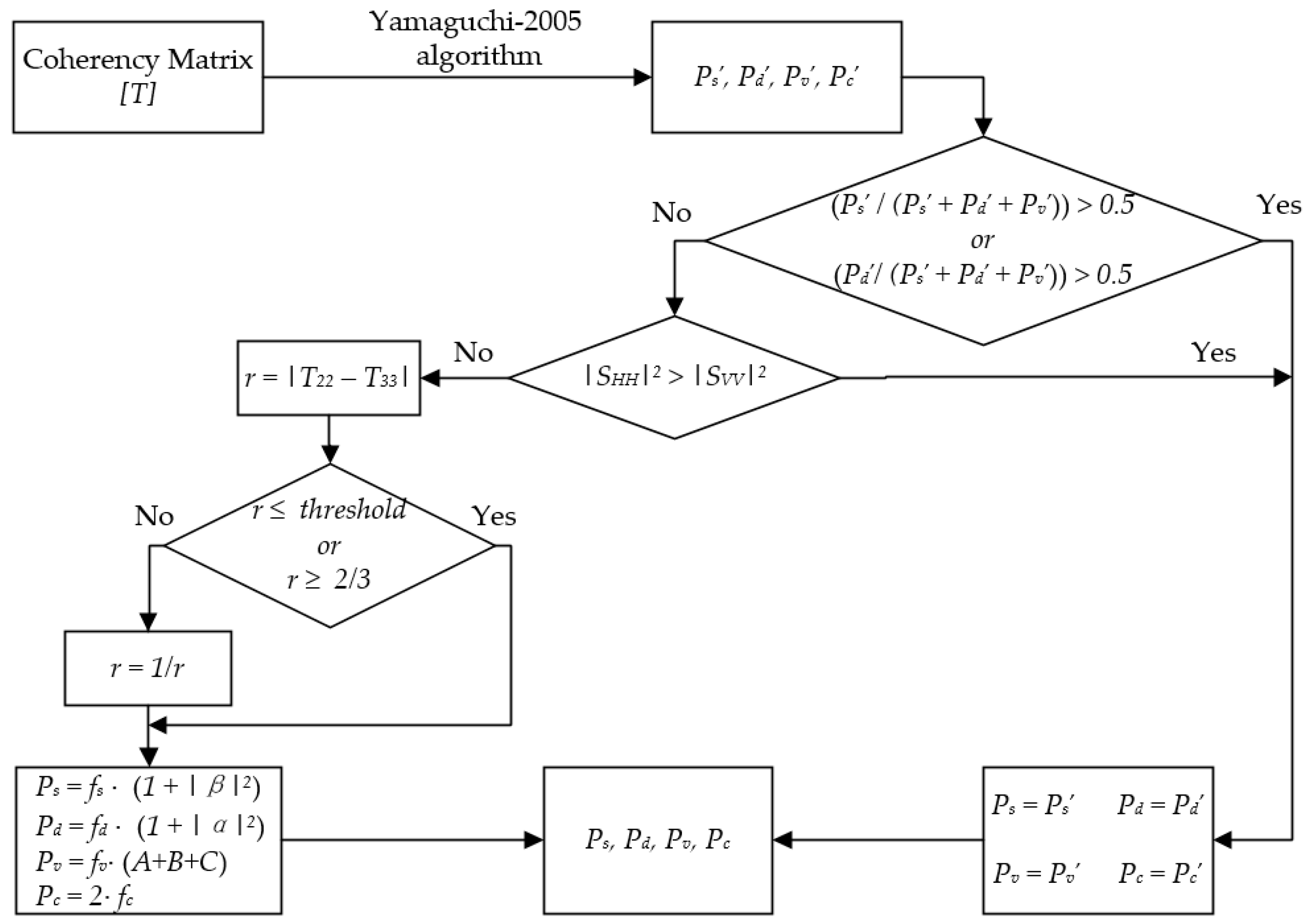
Figure 4.
Histograms of r values extracted from three squares in Figure 1a. The color of each histogram curve corresponds to the color of each square.
Figure 4.
Histograms of r values extracted from three squares in Figure 1a. The color of each histogram curve corresponds to the color of each square.

Figure 5.
Decomposition results of Goldstone AIRSAR data, USA using (a) the proposed algorithm and (b) Yamaguchi-2011 algorithm. In the figure, double-bounced scattering is shown in red color, volumetric scattering in green color, and surface scattering in blue color. Three trihedral corner reflectors (CRs) are numbered as 1 to 3, three dihedral CRs with AOAs of 0° as 4 to 6, and three dihedral CRs with AOAs of 45° as 7 to 9.

Figure 6.
Decomposition results of Oberpfaffenhofen E-SAR data, Germany. (a) The proposed algorithm and (b) the enlarged views of the red, blue, and green squares (as identified in Figure 1a). (c) The Yamaguchi-2011 algorithm and (d) enlarged views of the red, blue, and green squares.
Figure 6.
Decomposition results of Oberpfaffenhofen E-SAR data, Germany. (a) The proposed algorithm and (b) the enlarged views of the red, blue, and green squares (as identified in Figure 1a). (c) The Yamaguchi-2011 algorithm and (d) enlarged views of the red, blue, and green squares.

Figure 7.
Decomposed results of Vanceboro UAVSAR data, USA. (a) The proposed algorithm and (b) the Yamaguchi-2011 algorithm. The close-up views of a forest stand using the proposed algorithm (c) and the Yamaguchi-2011 algorithm (d). The enlarged views of the manufacture facility consisting of buildings and man-made structures using the proposed algorithm (e) and the Yamaguchi-2011 algorithm (f).

Figure 8.
Decomposed results of San Francisco PALSAR data, USA. (a) The proposed algorithm, and (b) Yamaguchi-2011 algorithm. (c) The enlarged view outlined by the red square and extracted from (a), and (d) the enlarged view within the red square and extracted from (b).
Figure 8.
Decomposed results of San Francisco PALSAR data, USA. (a) The proposed algorithm, and (b) Yamaguchi-2011 algorithm. (c) The enlarged view outlined by the red square and extracted from (a), and (d) the enlarged view within the red square and extracted from (b).
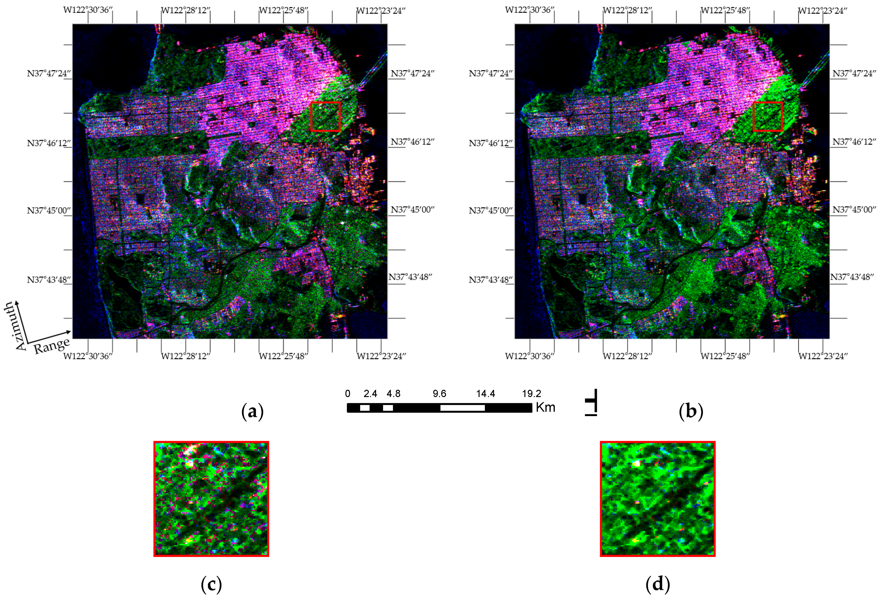
Figure 9.
(a–c) Histograms of three types of scattering mechanism extracted from a red square in Figure 8. The solid line stands for the proposed algorithm, and the dotted one for Yamaguchi-2011 algorithm.
Figure 9.
(a–c) Histograms of three types of scattering mechanism extracted from a red square in Figure 8. The solid line stands for the proposed algorithm, and the dotted one for Yamaguchi-2011 algorithm.


Table 1.
Summary of reviewed PolSAR decomposition models/algorithms on bases of decomposition approach, primary usage, and secondary usage.
Table 1.
Summary of reviewed PolSAR decomposition models/algorithms on bases of decomposition approach, primary usage, and secondary usage.
| Algorithm | Decomposition Approach | Primary Usage | Secondary Usage | Note |
|---|---|---|---|---|
| Du and Wang [1], and Chen et al. [23]. | Model component and coherence | Urban area | Forested environment | [1] is revised from [10]. [23] is revised from [8]. |
| Wang and Davis [6], van Zyl et al. [7], and Zou et al. [22]. | Eigenvalue and eigenvector | Forested environment | Urban area | |
| Yamaguchi et al. [5], Freeman and Durden [8], Freeman [9], Yamaguchi et al. [10], An et al. [11], Arii et al. [12], Antropov et al. [13], Huang et al. [14], Chen et al. [15], Hong and Wdowinski [16], Xiang et al. [17], and Xie et al. [18]. | Model component | Forested environment | Urban area | [5] is revised from [10]. [9] is a simplified version of [8]. [10] and [11] are revised from [8]. [13] is the generalization form of [8], [9], [10], and [11]. [14] is simplified from [12]. [15] uses four volumetric scattering models in [8], [10], and [11]. [16] and [17] are revised from [10]. [18] is a combination of [13], [14] and [15]. |
| Kajimoto and Susaki [19], Susaki and Kajimoto [20], and Azmedroub et al. [21]. | Model component and classification | Urban area | Forested environment | [19,20,21] are hybrid of decomposition and classification. |
| The proposed algorithm. | Model component | Urban area | This is a revised version of [10]. |
Table 2.
Percentage of each scattering type of nine corner reflectors (CRs) extracted from Goldstone AIRSAR data, USA. In each cell, the number in the first row and in bold font is the percentage of a scattering type derived from the proposed algorithm. The number in the second row and in regular font is the percentage of a scattering type derived from Yamaguchi-2011 algorithm. The italicized number in the third row is the difference of the first two rows.
| CR | 1 | 2 | 3 | 4 | 5 | 6 | 7 | 8 | 9 |
|---|---|---|---|---|---|---|---|---|---|
| Surface scattering | 98.1 | 98.7 | 99.8 | 0.2 | 0.6 | 0.3 | 0.8 | 9.5 | 4.5 |
| 98.1 | 98.6 | 99.8 | 0.5 | 0.6 | 0.6 | 2.8 | 3.2 | 1.5 | |
| 0.0 | 0.1 | 0.0 | −0.3 | 0.0 | −0.3 | −2.0 | 6.3 | 3.0 | |
| Double-bounced scattering | 1.8 | 0.3 | 0.2 | 96.1 | 99.3 | 98.3 | 72.1 | 64.1 | 53.6 |
| 1.8 | 0.3 | 0.2 | 99.3 | 99.4 | 98.0 | 6.0 | 14.2 | 0.3 | |
| 0.0 | 0.0 | 0.0 | −3.2 | −0.1 | 0.3 | 66.1 | 49.9 | 53.3 | |
| Volumetric scattering | 0.1 | 1.0 | 0.0 | 3.7 | 0.1 | 1.4 | 27.1 | 26.4 | 41.9 |
| 0.1 | 1.1 | 0.0 | 0.2 | 0.0 | 1.4 | 91.2 | 82.6 | 98.2 | |
| 0.0 | −0.1 | 0.0 | 3.5 | 0.1 | 0.0 | −64.1 | −56.2 | −56.3 |
Table 3.
Averaged percentages of Ps, Pd, and Pv extracted from Oberpfaffenhofen E-SAR data, Germany. In the table, α represents the proposed algorithm and β Yamaguchi-2011 algorithm. δ is the difference of results.
Table 3.
Averaged percentages of Ps, Pd, and Pv extracted from Oberpfaffenhofen E-SAR data, Germany. In the table, α represents the proposed algorithm and β Yamaguchi-2011 algorithm. δ is the difference of results.
| Ps/(Ps + Pd + Pv) | Pd/(Ps + Pd + Pv) | Pv/(Ps + Pd + Pv) | |||||||
|---|---|---|---|---|---|---|---|---|---|
| α | β | δ | α | β | δ | α | β | δ | |
| Red square | 32.2 | 31.2 | 1.0 | 59.0 | 57.7 | 1.1 | 8.8 | 11.1 | −2.3 |
| Green square | 27.2 | 26.9 | 0.3 | 27.1 | 26.8 | 0.3 | 45.7 | 46.2 | −0.5 |
| Blue square | 37.9 | 25.7 | 12.2 | 44.7 | 31.3 | 13.4 | 17.4 | 43.0 | −25.6 |
Table 4.
Processing time of the proposed algorithm (first row), the Yamaguchi-2011 algorithm (second row), and the Xie et al. algorithm [18] (third row). Unit: seconds.
Table 4.
Processing time of the proposed algorithm (first row), the Yamaguchi-2011 algorithm (second row), and the Xie et al. algorithm [18] (third row). Unit: seconds.
| 200 × 200 | 400 × 400 | 800 × 800 | 1600 × 1600 | |
|---|---|---|---|---|
| The proposed algorithm | 0.9 | 2.6 | 10.6 | 51.2 |
| Yamaguchi-2011 algorithm | 1.7 | 15.4 | 222.4 | 4133.4 |
| Xie et al. algorithm | 6699.8 | 26,500.0 | 102,170.0 | - a |
a The processing time took too long to be completed.
© 2017 by the authors. Licensee MDPI, Basel, Switzerland. This article is an open access article distributed under the terms and conditions of the Creative Commons Attribution (CC BY) license (http://creativecommons.org/licenses/by/4.0/).
Share and Cite
MDPI and ACS Style
Duan, D.; Wang, Y. An Improved Algorithm to Delineate Urban Targets with Model-Based Decomposition of PolSAR Data. Remote Sens. 2017, 9, 1037. https://doi.org/10.3390/rs9101037
AMA Style
Duan D, Wang Y. An Improved Algorithm to Delineate Urban Targets with Model-Based Decomposition of PolSAR Data. Remote Sensing. 2017; 9(10):1037. https://doi.org/10.3390/rs9101037
Chicago/Turabian StyleDuan, Dingfeng, and Yong Wang. 2017. "An Improved Algorithm to Delineate Urban Targets with Model-Based Decomposition of PolSAR Data" Remote Sensing 9, no. 10: 1037. https://doi.org/10.3390/rs9101037
Note that from the first issue of 2016, this journal uses article numbers instead of page numbers. See further details here.