Detection of Bivalve Beds on Exposed Intertidal Flats Using Polarimetric SAR Indicators


1
State Key Laboratory of Remote Sensing Science, Institute of Remote Sensing and Digital Earth, Chinese Academy of Sciences, Beijing 100101, China
2
University of Chinese Academy of Sciences, Beijing 100049, China
3
Institut für Meereskunde, Universität Hamburg, 20146 Hamburg, Germany
*
Author to whom correspondence should be addressed.
Remote Sens. 2017, 9(10), 1047; https://doi.org/10.3390/rs9101047
Submission received: 24 June 2017
/
Revised: 26 September 2017
/
Accepted: 10 October 2017
/
Published: 13 October 2017
(This article belongs to the Special Issue Ocean Remote Sensing with Synthetic Aperture Radar)
Abstract
:We propose new indicators for bivalve (oyster and mussel) beds on exposed intertidal flats, derived from dual-copolarization (HH + VV) TerraSAR-X, Radarsat-2, and ALOS-2 images of the German North Sea coast. Our analyses are based upon the Kennaugh element framework, and we show that different targets on exposed intertidal flats exhibit different radar backscattering characteristics, which manifest in different magnitudes of the Kennaugh elements. Namely, the inter-channel correlation’s real (K3) and imaginary (K7) part can be used to distinguish bivalve beds from surrounding sandy sediments, and together with the polarimetric coefficient (i.e., the normalized differential polarization ratio, K0/K4) they can be used as indicators for bivalve beds using multi-frequency dual-copolarization SAR data. Our results show that continuous bivalve bed monitoring is possible using dual-copolarimetric SAR acquisitions at all radar wavelengths.
Keywords:
bivalve beds; intertidal flats; Kennaugh elements; SAR; dual-polarization; multi-frequency
1. Introduction
Intertidal flats are coastal areas between the land and the open sea that are at risk due to climate change, sea level rise, marine pollution, and invasive species [1,2,3]. The German Wadden Sea is such a dynamic ecosystem, with a high economic and ecological value, and has been a UNESCO World Natural Heritage since 2009 [4]. Pacific oysters are an invasive species that has been rapidly spreading over large parts of the German Wadden Sea during the past decades, thereby having an impact on nutrient cycling, water filtration, and the entire coastal ecosystem [5]. Therefore, a frequent environmental monitoring of this entire area (approx. 4700 km2) is not only important, but also mandatory. However, in-situ measurements in tidal flats face many constraints, because of the repetitive flooding and the shallow water depth [6], and the development of reliable and automated techniques for an accurate classification (especially for bivalve beds) and for an assessment of their changes are strongly required.
Remote sensing is already regarded as a useful tool for the monitoring of intertidal flats. There have been many studies utilizing optical remote sensing techniques to detect oyster/mussel habitats, but the use of those sensors is limited by daytime and cloud coverage [7,8,9]. Moreover, bivalve beds are often covered by brown algae, which may cause classification errors when using optical data. In addition, there exist difficulties in describing the spectral signatures of bivalves due to a considerable spectral variability.
Radar sensors such as Synthetic Aperture Radar (SAR) can overcome those restrictions because of their all-weather capabilities and independence of daylight and also due to their ability to extract detailed structural information. It was found that bivalve beds and salt marshes have specific SAR signatures and can thus be monitored using space-borne SAR sensors [10,11,12,13]. Those bivalves are exposed above the sediments and form a rough reef or bed structure (with sharp and jagged surfaces) and increase the surface roughness locally, which causes stronger radar backscattering signals, making them visible in SAR imagery [11,14,15]. Therefore, surface roughness parameters retrieved from radar backscattering models can be used to distinguish bivalves from surrounding areas [10,16,17]. However, this approach may work only for a limited range of smooth bare soils, while mudflats with intense benthic fauna can be misinterpreted [13,14]. In addition, sandy sediments with sharp rims and rippled surfaces may also cause strong signals in SAR imagery, and hence SAR intensity channels cannot be simply used to get satisfactory classification accuracies.
With the advent of high-performance polarimetric SAR sensors, studies have been conducted to distinguish bivalves from sediments using multiple polarization SAR data. Gade et al. [10] provided both multi-frequency and multi-temporal analyses to improve the identification of bivalve beds in the German Wadden Sea. Similarly, Dehouck et al. [18] used combined TerraSAR-X (TSX) and optical imagery of the French Arcachon Bay to detect mussels, salt marshes, and sandy sediments. Choe et al. [14] demonstrated that quad polarimetric (quad-pol) multi-frequency (C-band and L-band) SAR data can be used to detect oyster reefs, but also demonstrated that indicators derived from L-band data show no significant differences between oyster beds and surrounding areas. Further analyses of indicators based on L-band data are rare, and therefore, the present paper is to propose polarimetric SAR indicators for the detection of bivalve beds that work at all wavelengths.
Commonly applied polarimetric decompositions such as the Cloude-Pottier and Freeman-Durden decomposition have been used for intertidal flats studies [19,20,21,22]. However, these decompositions can only be applied to quad-pol SAR data, while operational SAR sensors currently in orbit (such as the German TerraSAR-X, the Italian COSMO-SkyMed, and the European Sentinel-1A/B) provide data in dual-copolarization or dual-polarization mode. Radarsat-2 and ALOS-2 may acquire quad-pol data. However, this is only at the cost of limited spatial resolution and areal coverage. Moreover, bivalve beds on exposed intertidal flats can only be monitored at low tide. The limited time-window requires larger areal coverage with fine resolution. Therefore, further research is needed on the capabilities of existing or newly acquired dual-copolarization (dual-copol; HH + VV) SAR data [23] for monitoring intertidal flats, especially for the detection and classification of sediments and bivalve beds.
The Normalized Kennaugh element framework was developed by Schmitt et al. [24] and provides a method that can be applied on multi-scale, multi-temporal, multi-polarized, multi-frequency, and multi-sensor SAR data in a consistent mathematical manner. The Kennaugh elements allow the interpretation of physical scattering mechanisms (even- and odd-bounce scattering) for dual-polarization data [25], and this decomposition framework may allow a successful inclusion of those data into the Wadden Sea monitoring. Common polarimetric decompositions are either coherent or incoherent. The coherent decompositions based on the Sinclair matrix prohibit multi-looking and require descriptions of distributed targets, while the incoherent decompositions based on either the covariance or the coherency matrix often require large look numbers to keep radiometric stability [23,24,25]. Therefore, the Kennaugh formulation appears to be the right balance due to the basic description of the backscattering process [24]. Schmitt et al. and Moser et al. [25,26] first applied Kennaugh elements into wetland monitoring using dual-copol SAR data of the Upper Rhine in Germany and Lac Bam in Burkina Faso, respectively. Gade et al. [11] showed that the polarization coefficient (i.e., the normalized differential polarization ratio, referred to as PC) can be used to infer indicators for bivalve beds and demonstrated with X-band data. In this paper, we follow on those works using, among others, TerraSAR-X (TSX), Radarsat-2 (RS2), and ALOS-2 (AL2) data, with the specific aim to propose indicators for bivalve beds that were derived from dual-copol SAR data acquired at all wavelengths (X-, C-, and L-band).
The test site in the German Wadden Sea and the dual-copol multi-frequency (X-, C-, and L-band) SAR datasets are introduced in the following Section. The Kennaugh element framework and polarization coefficient are described thereafter, along with a presentation of statistical parameters that were used for the detection of oyster and mussel beds. We then compare and discuss the results of three space-borne sensors (working at X-, C-, and L-band) using the available dual-copol data and finally draw some conclusions.
2. Materials and Methods
2.1. Test Site and SAR Data
The test site “Amrum” on the northern part of the German Wadden Sea (Figure 1) is located between the islands of Amrum and Föhr and was already subject to previous studies [11,12,27]. This region contains sandy and muddy sediments, vegetated areas, bivalve beds (mainly Pacific oysters and cockles, but also blue mussels) and seagrass meadows; hence it represents an area of a typical mixture of bivalve beds and sediments on exposed intertidal flats. In addition, the bivalve beds in the test area “Amrum” are quite stable and chosen for demonstrating the effectiveness of the following indicators. Blue mussels and Pacific oysters may form extensive bivalve beds on elevated intertidal flats that may also contain areas of bare sediments and water puddles.
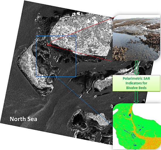
Frequent monitoring of bivalve beds in the test site “Amrum” is conducted during field campaigns as well as based on optical and (single-polarization) SAR imagery [12]. Therefore, a larger number of SAR images was available for the present investigation. The solid rectangles in Figure 1 delineate the locations of the X-, C-, and L-band SAR data used in this study. VV-polarization SAR scenes acquired around low tide by TSX, RS2, and AL2 are shown in Figure 2 as examples. Herein we focused on an 8.97 km × 8.31 km area of interest within the “Amrum” test site, marked by the red rectangle in the upper panel of Figure 2. In all panels, bivalve beds on exposed sediments show up as bright patches. That is because the bivalves stick out of the sediments, increasing the surface roughness locally with higher radar backscattering. Some of the exposed sediments in the inner parts of the intertidal flats appear in dark, likely because of remnant water that effectively flattens the surface. Tidal creeks can be delineated because of their rather smooth surface causing lower radar backscatter and also due to the enhanced surface roughness of the sandy sediments at their rims. As seen in Figure 2, it is difficult to infer the spatial extent of bivalve beds simply using intensity channels. This motivated us to use polarimetric information available at all wavelengths (X-, C-, and L-band).
Three single-look complex (SLC) SAR images of the test site “Amrum” acquired around low tide by TSX, RS2, and AL2 were used for the analyses presented in this paper. The SAR images’ pixel sizes range from 1 m × 1 m to 5 m × 5 m. Details of the used SAR images are summarized in Table 1, including the acquisition dates and times, the sensors and frequencies, polarizations, incidence angles, and water levels measured by the tide gauge “Wittdün” on the southern tip of Amrum. The TSX image was acquired in High-Resolution Spotlight mode (dual-copol: HH + VV), the RS2 image in Fine Quad-Pol mode (quad-pol: HH + HV + VH + VV), and the AL2 image in Strip-Map Ultra-Fine mode (quad-pol: HH + HV + VH + VV). However, as our analyses were carried out with the specific aim to demonstrate the potential of dual-copol SAR images for bivalve bed detection, we only used the co-polarization (HH and VV) channels of the RS2 and AL2 data. All SAR images were acquired close to the low tide (around 30 min) and at comparable incidence angles (between 30° and 40°). Validation data was obtained during field excursions in 2015.
For the validation of our results, we used in-situ data from monitoring campaigns in 2015 provided by the local National Park Agency. The left panel of Figure 3 shows the VV-pol TSX SAR image, with both Amrum on the left and Föhr on the upper right masked out for better orientation. Figure 3 also shows that many parts of the exposed intertidal flats appear brighter, although not all of them are bivalve beds.
Figure 4 shows transects of the normalized radar cross section (NRCS) of the three SAR image along the yellow line in the right panel of Figure 3 (solid curves; blue: TSX; red: RS2; green: AL2). Also added as dashed-dotted lines are the respective noise floors at vertical polarization, the noise equivalent sigma zero (NESZ). Hereafter, we used only those data whose signal-to-noise ratio (SNR) was at least 2 dB. From Figure 4, we can see that at most places, the NRCS was well above the noise floor; however, we also note that at some places the backscattered signal dropped below the noise floor, particularly at L-band (green curve/line).
2.2. Kennaugh Element Framework
The single-look complex (SLC) TSX, RS2, and AL2 products were processed following a general approach that is based upon the elements extracted from the 4 × 4 Kennaugh matrix, [K], which is computed by linearly transforming the four-dimensional Stokes vector [24]:
The Kennaugh element framework has been demonstrated to be applicable to dual- as well as quad-pol data of any wavelengths. In this study, we used dual-copol (HH + VV) TSX data, from which only the Kennaugh elements K0, K3, K4, and K7, can be inferred as follows [24]:
where |Spp|2 are the image intensities at polarization pp, the asterisk (*) denotes the complex conjugate, and the factor appears for symmetry reasons. K0 reflects the total intensity of both HH and VV layers; K3 is the difference between even- and odd-bounce scattering, where large values indicate a stronger even-bounce scattering than odd-bounce scattering, and vice versa [24]; K4 is the difference between the HH and VV intensities; K7 is the phase shift between even- and odd-bounce scattering. In the case of a dual-pol system (one co-pol and one cross-pol channel) Equations (2) to (5) correspond exactly to the well-known definition of a Stokes vector.
Following [24], the Kennaugh element layers were subsequently multi-looked, calibrated, and ground-range projected (UTM Zone 32, 1 m pixel spacing). These four Kennaugh elements at all wavelengths are shown in Figure 5. In this paper, we use the normalized Kennaugh elements, divided by the total intensity K0, in order to derive nearly normally distributed values per Kennaugh element and physically comparable measurements. Here, we choose the normalized K3 and K7, for detecting oysters and mussels.
Moreover, we use the polarization coefficient (PC), which was recently used by Gade et al. [11] as a promising parameter to infer indicators for bivalve beds from X-band dual-copol SAR images. PC is defined as
and is identical to the normalized Kennaugh element of K4.
Where the radar backscattering at horizontal polarization strongly dominates over that at vertical polarization PC approaches +1, and −1 in the opposite case. PC is close to 0 where the radar backscatter at both polarizations is similar. In this paper, we further verified the use of PC with respect to its effectiveness in detecting bivalve beds not only using X-band data as previous works, but also using data at longer radar wavelengths (C- and L-band).
3. Results
The new SAR decomposition framework described above was applied to the three SAR data sets of the test site “Amrum” in two case studies, the first of which were analyses of the real (K3) and imaginary (K7) parts of the inter-channel correlations, and the second analyses of PC using longer radar wavelengths (C- and L-band). In both case studies, we focused on potential indicators of bivalve beds.
3.1. New Indicators from Single Kennaugh Elements
The dielectric constant of bivalve shells (with lower moisture contents) is lower than that of the surrounding sediments, which would result in a lower radar backscatter from bivalve beds. However, since the bivalves are sticking out of sediments, they increase the surface roughness strongly, which in turn causes an overall stronger radar backscatter. And since they are oriented heterogeneously, this increase in radar backscatter depends on the radar polarization, which is the main factor that causes different polarimetric scattering signatures between bivalves and mudflats.
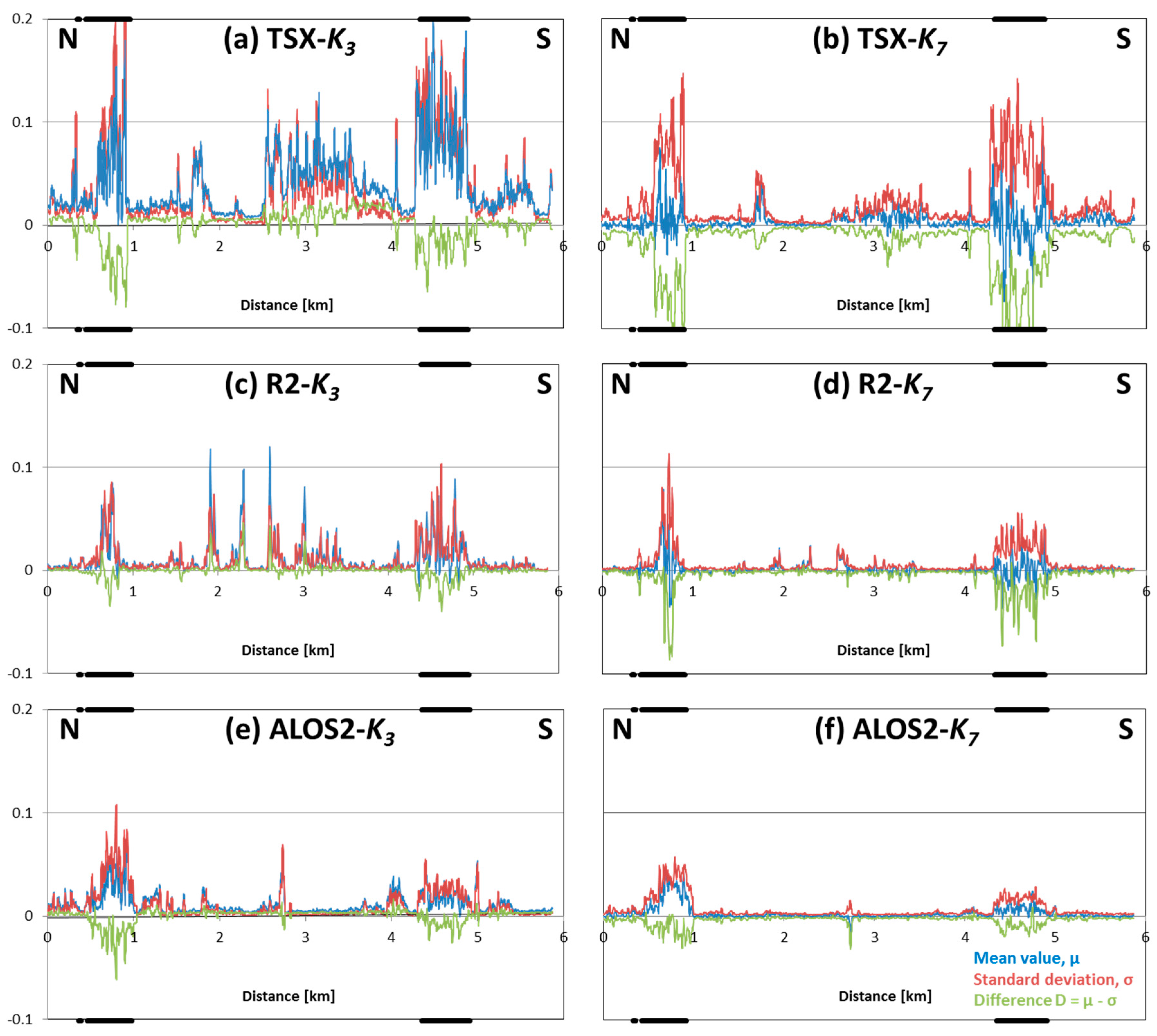
Along the transect line added to Figure 3 and Figure 5 (from north to south) we calculated profiles of the normalized Kennaugh elements K3 and K7. Figure 6 shows in blue the running mean, µ, of a moving 11-pixel window, in red the corresponding running standard deviation, σ, for K3 (left column) and K7 (right column) and for the TSX, RS2, and AL2 data (from top to bottom). In addition, we added in green the difference D of both,
Thick horizontal bars on the abscissae in Figure 6 denote the locations of bivalve beds, as found during field campaigns in 2015.
The panels in the left column (K3) of Figure 6 clearly show that in all radar bands both the (running) mean and (running) standard deviation are increased in the bivalve beds (between 0 km and 1 km, and between 4 km and 5 km), but also in the exposed sand flats in between. This effect is most pronounced in X-band (TSX, upper row) and weakens with increasing radar wavelength (middle row: RS2/C-band; lower row: AL2/L-band). However, we also note that the bivalve beds are the only areas where the standard deviation exceeds the mean value, which results in a negative difference D (green curves). This effect can be used to infer indicators for bivalve beds.
The peaks of the mean values indicate that both oyster/mussel beds and the sandy rims of the intertidal flats show stronger even-bounce backscatter components than odd-bounce, because of their rougher surfaces. This increase in K3 can be caused by either an increase in the even-bounce scattering or by a decrease in the odd-bounce scattering. In contrast, lower K3 values in the surrounding areas, consisting of mudflats and tidal channels, indicate much smoother surfaces. Apparently, the heterogeneous surface structure of bivalves causes a strong spatial variability of even- and odd-bounce backscattering and therefore higher standard deviations, which in turn results in negative differences, D3.
The Kennaugh element K7 holds complementary correlation information, the phase shift between even- and odd-bounce backscattering. The corresponding profiles in Figure 6 (right column) show that the phase differences inside the bivalve beds are always larger, and always show strong variations, so that the running standard deviation always exceeds the running mean. Therefore, the difference of both, D7, is always negative, but extreme values are only found in the bivalve beds. The rougher surfaces of bivalves cause diffuse radar backscattering, resulting in strong variations of the phase differences and, therefore, in standard deviations exceeding the mean values. Similar to the profiles in the left column of Figure 6, this effect weakens with increasing wavelength, i.e., from top to bottom. However, since areas of extremely negative “running differences” D7 correspond well with the validation data, we conclude that this difference can also be used as indicator for bivalve beds.
The profiles for both Kennaugh elements, K3 and K7 (left and right column of Figure 6, respectively), show a strong dependence on radar wavelength: with increasing wavelength (i.e., from top to bottom in Figure 6), the curves become flatter, i.e., the difference between even- and odd-bounce backscattering becomes smaller. One possible reason lies in the size of oysters, which are the prevailing species in those beds: depending on their age, the oysters may become 30 cm long, with the majority being below 20 cm in length. The roughness scale of those beds, therefore, is on the order of a decimeter, and the beds’ surfaces are much rougher for an X-band sensor (wavelength 3 cm) than for an L-band sensor (25 cm). This also results in smaller differences in the polarimetric backscattering, i.e., in smaller differences between even- and odd-bounce backscattering. Another, though less important, reason may lie in the season, in which the SAR data were acquired: the TSX data were acquired in early summer (June), during the vegetation period and growing season of the bivalves, while both the C- and L-band data were acquired in winter (December and February, respectively), when storm and high water events are more frequent.
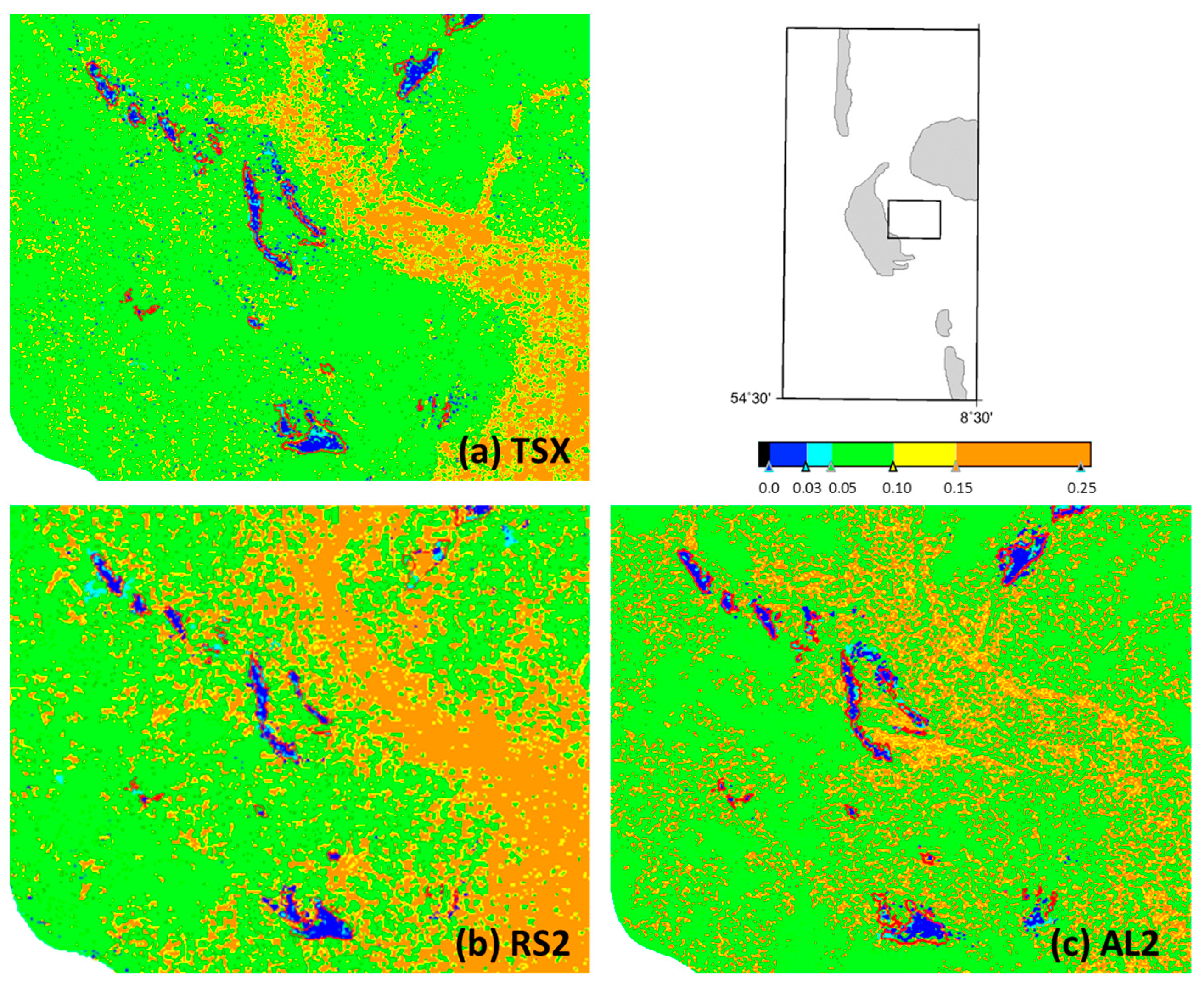
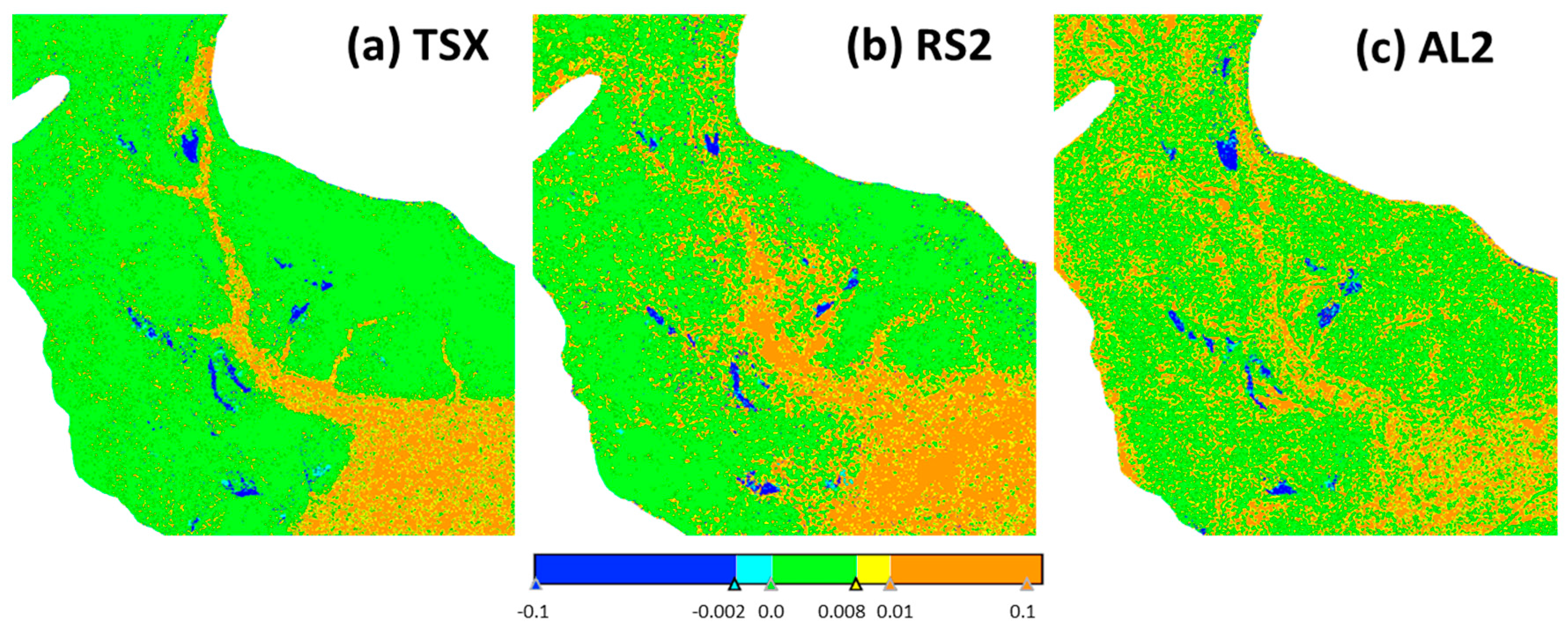
In order to generate maps of bivalve bed indicators we calculated the running mean and standard deviation of a moving 11 pixels × 11 pixels window, and consequently the differences D3 (Figure 7) and D7 (Figure 8). For D3 we set 0 as threshold for the bivalve indicators (i.e., we marked all negative differences D3), and we arbitrarily chose 0.01 to further discriminate between sediments (between 0 and 0.01) and tidal channels and creeks (above 0.01). The results for the three datasets, TSX, RS2, and AL2, are shown in Figure 7, where the blue, orange, and green colors denote bivalve beds, exposed sediments, and tidal channels and creeks, respectively. A comparison with the validation data (red lines in Figure 3) immediately reveals that the difference D3 provides an indicator for bivalve beds on exposed intertidal flats. Moreover, previous studies have also demonstrated that the use of multi-polarization SAR images have some additional potential for the monitoring of sediment surfaces on intertidal flats using SAR sensors [6,11,18,22]. With the given color coding, areas of water coverage, mainly the tidal channels, appears in orange colors, whereas the open sediment flats appear in green and yellow. More research is still required to analyze to what extent this parameter can be used in this respect.
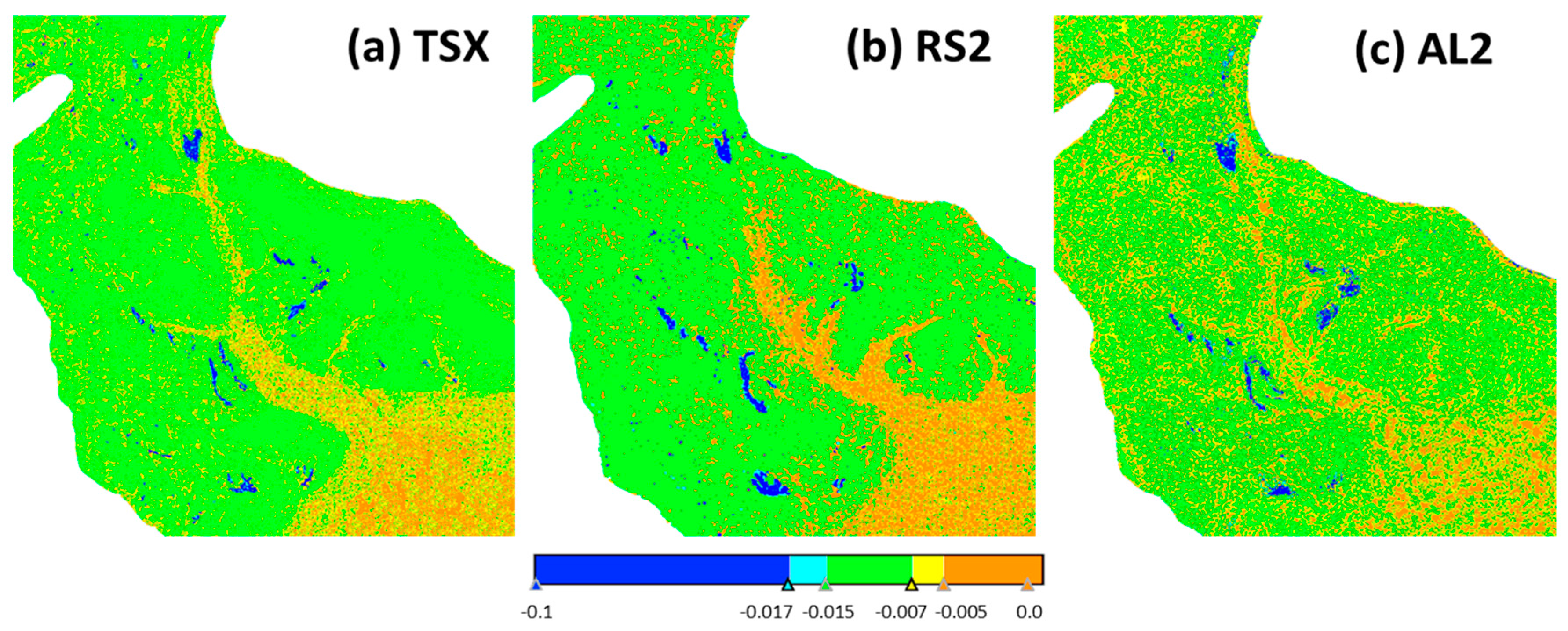
The same analyses were also performed with the difference D7 (Figure 8), with the thresholds set to −0.015 (bivalves–sediment) and −0.005 (sediment–tidal creeks and channels). The results look very similar to those obtained for D3 (Figure 7).
Figure 7 and Figure 8 demonstrate that the best correlation with the in-situ data is obtained when X-band data are used, and the indicators for bivalves are derived using the Difference D3 (left Panel of Figure 7). This is in line with our earlier observation, that the highest K3 values of the running mean and standard deviation were found at X-band (upper left panel of Figure 6). The detection accuracy was derived as the ratio of the number of pixels correctly assigned to bivalve beds and the total number of pixels in bivalve beds, as given in the validation data from monitoring campaigns. The accuracies ranging from 84.70% to 88.87% for D3 and 81.02% to 85.13% for D7, are given in Table 2. Moreover, a discrimination of exposed sediments (green) and tidal creeks and channels (orange) also appears to be possible using our approach, particularly using X-band data and the difference D3. The most homogeneous backscattering conditions are found in water-covered areas, i.e., in the tidal creeks and channels, and as a result, the difference of tidal channels and exposed sediment flats between the running mean and standard deviation is maximum in those areas. Apparently, this discrimination works well at short radar wavelengths (X-band), although we also note that different water levels (Table 1) may have caused the observed differences.
3.2. Indicators from Polarization Coefficients
The polarization coefficient (PC) was used by Gade et al. [11,28] as indicator for bivalve beds on exposed intertidal flats. As the abrupt end of the ALOS-1 mission in 2011, we were only able to demonstrate PC with TSX X-band data. Here, we build up on those previous works using SAR data acquired at longer wavelengths (C- and L-band). Following [11] the product P is defined as
where and are the absolute value of the running mean and standard deviation, respectively, of the polarization coefficient, PC. Because of their increased surface roughness, bivalve beds always cause an increased radar backscatter at both HH and VV polarizations, resulting in both low mean values and low standard deviations, and eventually in low values of the product P [11]. Similar to the above analyses, we used a running window of size 11 pixels × 11 pixels to calculate the product P, and the results are shown in Figure 9.
Figure 9 shows that the spatial range of the bivalve beds coincides well with the validation data of the field campaigns (marked in red). We note that the high detection accuracies for the Product P (84.72% to 87.72%) indicate that the use of dual co-pol SAR images has good potential for the monitoring of bivalves even when SAR data acquired at longer wavelengths (L-band) are used. Similar to the above findings, we found that the ability to distinguish sediments from tidal creeks and channels decreases with increasing radar wavelength. It should also be noted that surface scattering is the dominant scattering mechanism in most areas of exposed intertidal flats and the adjacent tidal creeks and channels. As the radar wavelength increases, these surface scatters tend to represent a relatively smoother effect, which can also explain this phenomenon. Moreover, images acquired at incidence angles between 31° and 37° are well suited for detection of bivalve beds because of the stronger radar contrast between the bivalve beds and their surroundings.
4. Discussion
Our studies indicate that the use of the Kennaugh element framework has great potential for the detection of bivalve beds on exposed intertidal flats. The spatially complex and rough surface structures of bivalve (oyster/mussel) beds on intertidal flats can be clearly defined through their unique polarimetric signatures, so that they can be discriminated from the surrounding bare sediments. A major advantage of the proposed indicators is that a series of single-acquisition SAR data can be used for a frequent monitoring of intertidal flats on the German North Sea coast, thereby providing valuable input for existing classification schemes that is independent of daylight and weather conditions. The detection of bivalve beds based on the Kennaugh element framework works best using X-band SAR data, but even long radar wavelengths (L-band) can be used to gain reliable results, and thus complement the L-band’s inability to distinguish bivalves from surrounding areas in previous studies.
The Kennaugh element framework appears to be superior over other decomposition schemes on quad-pol SAR data and thus, improves the monitoring capabilities in the German Wadden Sea, particularly during the short periods of low tide. E.g., decompositions based on eigenvectors are susceptible to mixed results in very noisy decomposition parameters and thus, require very high look numbers to overcome this problem. Decompositions applied to interpret the components with the help of physical mechanisms based on radar backscattering models potentially also impair the description of natural targets, and are always limited to certain wavelength regimes. The numerical models, in turn, can rare suffice our requirements in wide range of smooth bare soils in the German Wadden Sea, especially targets with vegetation coverage, as well as our existing or newly acquired dual-copol SAR datasets. In this study, the relationship between even- and odd-bounce scattering events helps the detection of bivalves as expected, especially the complementary phase shift between even- and odd-bounce scattering (K7). It was physically interpreted herein and demonstrated the ability to aid the discriminability between bivalve beds and surrounding sediments. Therefore, the Kennaugh decomposition theory has great advantages in describing the scattering features of sediments and habitats on exposed intertidal flats and may help in fully understanding the radar backscattering mechanisms on those flats. This Kennaugh-based approach should be transferable to any other regions as long as the data acquired at low tide, likewise to any other available polarimetric SAR sensors in orbit (such as COSMO-SkyMed and Sentinel-1A/B). This transferable to our available SAR datasets in terms of different wavelengths and characteristics is subject to ongoing research. This is in line with the idea exploited in this paper and could be further extended to other intertidal flats, such as the test sites around the islands of Spiekeroog and Norderney in the German Wadden Sea.
We also note that our results may help in improving the results from field campaigns: not only were our thresholds for the discrimination of bivalve beds, sediments, and tidal creeks and channels chosen arbitrarily, but the borders of the bivalve beds measured in-situ are always subjectively identified and may not reflect the very density threshold, from which bivalves may be detectable from space. In addition, our results also provide predictive guidance for the future field campaigns, based on multi-frequency SAR data and on multi-polarization modes. In this way, frequent monitoring of targets on exposed intertidal flats can be conducted combining the rapid imaging of SAR instruments with field investigations. It should be mentioned that dedicated field campaigns can be conducted only once or twice per year because of the reduced accessibility of these areas. In addition, muddy sediments and tidal channels may impede field surveys of larger areas or their access from land. Thus, such manpower- and time-consuming field campaigns cannot be conducted frequently, and this is also one of our motivations to monitor habitats using remote sensing techniques.
Any discrimination between different bivalve species (e.g., between blue mussels and oysters, or between cockles and oysters) based on polarimetric SAR images is not (yet) possible and requires further analyses. Therefore, further research is still needed to determine to what extent our new parameters can be used for such purposes. In addition, different water levels and seasonal changes can influence the backscattering characteristics of bare sediments [29] and bivalve beds. Therefore, future work will also include the sensitivity of Kennaugh elements to water levels and seasonal changes, e.g., the coverage by brown algae or Fucus. Future studies will be performed using dual-polarization SAR data (with one co-polarization and one cross-polarization channel), as usually acquired in current (Sentinel-1A/B) and future (RCM and SAOCOM) space borne SAR missions.
5. Conclusions
We have introduced new polarimetric SAR indicators for bivalve beds on exposed intertidal flats that are based on dual-copol SAR data. The proposed indicators for bivalve beds consist of the normalized real (K3) and imaginary (K7) parts of inter-channel correlations, as well as on the polarization coefficient, i.e., the normalized differential polarization ratio, PC = K4/K0. Comparing with the in-situ data from the field campaigns, we conclude that the Difference D3 and D7, as well as Product P, are useful indicators for extracting backscattering characteristics of bivalve beds, and can provide frequent and accurate mapping of habitats on intertidal flats.
Using SAR data from different sensors (working at different radar bands) the locations of the newly applied indicators always coincided with those where bivalve beds were encountered during field campaigns. Therefore, we also conclude that bivalve (oyster/mussel) beds can be detected at all radar wavelengths (X-, C-, and L-band), although we note that best results were obtained using X-band (TSX) data. In addition, the proposed indicators work well using images acquired at incidence angles between 31° and 37°.
Our proposed indicators allow the dual-copol SAR datasets for the detection of bivalve beds, exploiting the values of the existing or newly acquired datasets from the SAR sensors in orbit to the largest extent and keeping fine spatial resolution and large areal coverage. Moreover, the fact that these indicators are based on single-acquisition SAR data makes it superior to others based on series of SAR images, particularly for the monitoring of intertidal flats, a highly dynamic environment. Therefore, the results of our polarimetric analyses, as presented herein, have great potential to act as valuable input for existing classification systems.
Acknowledgments
The authors are grateful to Jörn Kohlus and Kai Eskildsen of the National Park Agency of the Schleswig-Holsteinean Wadden Sea National Park, who provided a-priori knowledge and in-situ data. One of the authors (W.W.) performed this research is in the frame of a fellowship of the German Academic Exchange Service (DAAD). Tide gauge data were provided by the Waterways and Shipping Board (Wasser- und Schifffahrtsamt, WSA) Tönning. ALOS-2, Radarsat-2, and TerraSAR-X data were provided by JAXA, CSA, and DLR, respectively, under contract RA6-3200 and 5077/OCE0994. RADARSAT is an official mark of the Canadian Space Agency. This work was also supported in part by the National Key R & D Program of China under Grant 2017YFB0502803 and in part by the Student President Foundation of the Institute of Remote Sensing and Digital Earth under Grant Y6SY1400CX.
Author Contributions
W. Wang, M. Gade, and X. Yang conceived and designed the data analyses; W. Wang mainly performed the analyses and interpretation of the results, and wrote most sections of this paper; M. Gade acquired the data, participated in analyses and interpretation, and contributed in writing and revising the paper. X. Yang aided with revising the manuscript. The sequence of authors reflects their level of contribution.
Conflicts of Interest
The authors declare no conflict of interest.
References
- Troost, K. Causes and effects of a highly successful marine invasion: Case-study of the introduced Pacific oyster Crassostrea gigas in continental NW European estuaries. J. Sea Res. 2010, 64, 145–165. [Google Scholar] [CrossRef]
- Lee, Y.K.; Park, J.W.; Choi, J.K.; Oh, Y.; Won, J.S. Potential uses of TerraSAR-X for mapping herbaceous halophytes over salt marsh and tidal flats. Estuar. Coast. Shelf Sci. 2012, 115, 366–376. [Google Scholar] [CrossRef]
- Klemas, V. Remote sensing of emergent and submerged wetlands: An overview. Int. J. Remote Sens. 2013, 34, 6286–6320. [Google Scholar] [CrossRef]
- Van der Wal, D.; Herman, P.M.J. Regression-based synergy of optical, shortwave infrared and microwave remote sensing for monitoring the grain-size of intertidal sediments. Remote Sens. Environ. 2007, 111, 89–106. [Google Scholar] [CrossRef]
- Regniers, O.; Bombrun, L.; Ilea, I.; Lafon, V.; Germain, C. Classification of oyster habitats by combining wavelet-based texture features and polarimetric SAR descriptors. In Proceedings of the IEEE International Geoscience and Remote Sensing Symposium, Milan, Italy, 26–31 July 2015. [Google Scholar]
- Gade, M.; Alpers, W.; Melsheimer, C.; Tanck, G. Classification of sediments on exposed tidal flats in the German Bight using multi-frequency radar data. Remote Sens. Environ. 2008, 112, 1603–1613. [Google Scholar] [CrossRef]
- Liu, S.; Li, Z.; Yang, X.; William, G.P.; Yu, Y.; Zheng, Q.; Li, X. Atmospheric frontal gravity waves observed in satellite SAR images of the Bohai Sea and Huanghai Sea. Acta Oceanol. Sin. 2010, 29, 35–43. [Google Scholar] [CrossRef]
- Grizzle, R.E.; Adams, J.R.; Walters, L. Historical changes in intertidal oyster (Crassostrea Virginica) reefs in a Florida Lagoon potentially related to boating activities. J. Shellfish Res. 2002, 21, 749–756. [Google Scholar]
- Zheng, Q.; Holt, B.; Li, X.; Liu, X.; Zhao, Q.; Yuan, Y.; Yang, X. Deep-water seamount wakes on SEASAT SAR image in the Gulf Stream region. Geophys. Res. Lett. 2012, 39, 11604. [Google Scholar] [CrossRef]
- Gade, M.; Melchionna, S.; Stelzer, K.; Kohlus, J. Multi-frequency SAR data help improving the monitoring of intertidal flats on the German North Sea coast. Estuar. Coast. Shelf Sci. 2014, 140, 32–42. [Google Scholar] [CrossRef]
- Gade, M.; Melchionna, S. Joint use of multiple Synthetic Aperture Radar imagery for the detection of bivalve beds and morphological changes on intertidal flats. Estuar. Coast. Shelf Sci. 2016, 171, 1–10. [Google Scholar] [CrossRef]
- Müller, G.; Stelzer, K.; Smollich, S.; Gade, M.; Adolph, W.; Melchionna, S.; Kemme, L.; Geißler, J.; Millat, G.; Reimers, H.C. Remotely sensing the German Wadden Sea—A new approach to address national and international environmental legislation. Environ. Monit. Assess. 2016, 188, 595. [Google Scholar] [CrossRef] [PubMed]
- Choe, B.H.; Kim, D.J.; Hwang, J.H.; Oh, Y.; Moon, W.M. Oyster reef signature in tidal flats detected by multi-frequency polarimetric SAR data. In Proceedings of the IEEE International Geoscience and Remote Sensing Symposium, Vancouver, BC, Canada, 24–29 July 2011. [Google Scholar]
- Choe, B.H.; Kim, D.J.; Hwang, J.H.; Oh, Y.; Moon, W.M. Detection of oyster habitat in tidal flats using multi-frequency polarimetric SAR data. Estuar. Coast. Shelf Sci. 2012, 97, 28–37. [Google Scholar] [CrossRef]
- Baghdadi, N.; Zribi, M.; Loumagne, C.; Ansart, P.; Anguela, T.P. Analysis of TerraSAR-X data and their sensitivity to soil surface parameters over bare agricultural fields. Remote Sens. Environ. 2008, 112, 4370–4379. [Google Scholar] [CrossRef]
- Park, S.E.; Moon, W.M.; Kim, D.J. Estimation of surface roughness parameter in intertidal mudflat using airborne polarimetric SAR data. IEEE Trans. Geosci. Remote Sens. 2009, 47, 1022–1031. [Google Scholar] [CrossRef]
- Van der Wal, D.; Herman, P.M.J.; van den Dool, A.W. Characterisation of surface roughness and sediment texture of intertidal flats using ERS SAR imagery. Remote Sens. Environ. 2005, 98, 96–109. [Google Scholar] [CrossRef]
- Dehouck, A.; Lafon, V.; Baghdadi, N.; Roubache, A.; Rabaute, T. Potential of TerraSAR-X imagery for mapping intertidal coastal wetlands. In Proceedings of the 4th TerraSAR-X Science Team Meeting, Oberpfaffenhofen, Germany, 14–16 February 2011. [Google Scholar]
- Van Beijma, S.; Comber, A.; Lamb, A. Random forest classification of salt marsh vegetation habitats using quad-polarimetric airborne SAR, elevation and optical RS data. Remote Sens. Environ. 2014, 149, 118–129. [Google Scholar] [CrossRef]
- Lee, S.K.; Hong, S.H.; Kim, S.W.; Yamaguchi, Y.; Won, J.S. Polarimetric features of oyster farm observed by AIRSAR and JERS-1. IEEE Trans. Geosci. Remote Sens. 2006, 44, 2728–2735. [Google Scholar] [CrossRef]
- Cheng, T.Y.; Yamaguchi, Y.; Chen, K.S.; Lee, J.S.; Cui, Y. Sandbank and oyster farm monitoring with multi-temporal polarimetric SAR data using four-component scattering power decomposition. IEICE Trans. Commun. 2013, 96, 2573–2579. [Google Scholar] [CrossRef]
- Wang, W.; Yang, X.; Li, X.; Chen, K.; Liu, G.; Li, Z.; Gade, M. A fully polarimetric SAR imagery classification scheme for mud and sand flats in intertidal zones. IEEE Trans. Geosci. Remote Sens. 2017, 55, 1734–1742. [Google Scholar] [CrossRef]
- Ullmann, T.; Schmitt, A.; Jagdhuber, T. Two component decomposition of dual polarimetric HH/VV SAR data: Case study for the tundra environment of the Mackenzie Delta region, Canada. Remote Sens. 2016, 8, 1027. [Google Scholar] [CrossRef]
- Schmitt, A.; Wendleder, A.; Hinz, S. The Kennaugh element framework for multi-scale, multi-polarized, multi-temporal and multi-frequency SAR image preparation. ISPRS J. Photogramm. Remote Sens. 2015, 102, 122–139. [Google Scholar] [CrossRef]
- Moser, L.; Schmitt, A.; Wendleder, A.; Roth, A. Monitoring of the Lac Bam wetland extent using dual-polarized X-band SAR data. Remote Sens. 2016, 8, 302. [Google Scholar] [CrossRef]
- Schmitt, A.; Wendleder, A.; Roth, A.; Brisco, B. Water extent monitoring and water level estimation using multi-frequency, multi-polarized, and multi-temporal SAR data. In Proceedings of the IEEE International Geoscience and Remote Sensing Symposium, Quebec, QC, Canada, 13–18 July 2014. [Google Scholar]
- Gade, M.; Melchionna, S.; Kemme, L. Analyses of multi-year Synthetic Aperture Radar imagery of dry-fallen intertidal flats. In Proceedings of the 36th International Symposium of Remote Sensing and Environment, Berlin, Germany, 11–15 May 2015. [Google Scholar]
- Gade, M. A polarimetric radar view at exposed intertidal flats. In Proceedings of the IEEE International Geoscience and Remote Sensing Symposium, Beijing, China, 10–15 July 2016. [Google Scholar]
- Gade, M.; Wang, W.; Kemme, L. On the imaging of exposed intertidal flats by dual-polarization Synthetic Aperture Radar. Remote Sens. Environ. 2017. under review. [Google Scholar]
Figure 1.
The test site “Amrum” in the German Wadden Sea. The solid rectangles delineate the spatial coverage of the TerraSAR-X (TSX) (red), Radarsat-2 (RS2) (green), and ALOS-2 (AL2) (blue) data (Figure 2).
Figure 1.
The test site “Amrum” in the German Wadden Sea. The solid rectangles delineate the spatial coverage of the TerraSAR-X (TSX) (red), Radarsat-2 (RS2) (green), and ALOS-2 (AL2) (blue) data (Figure 2).
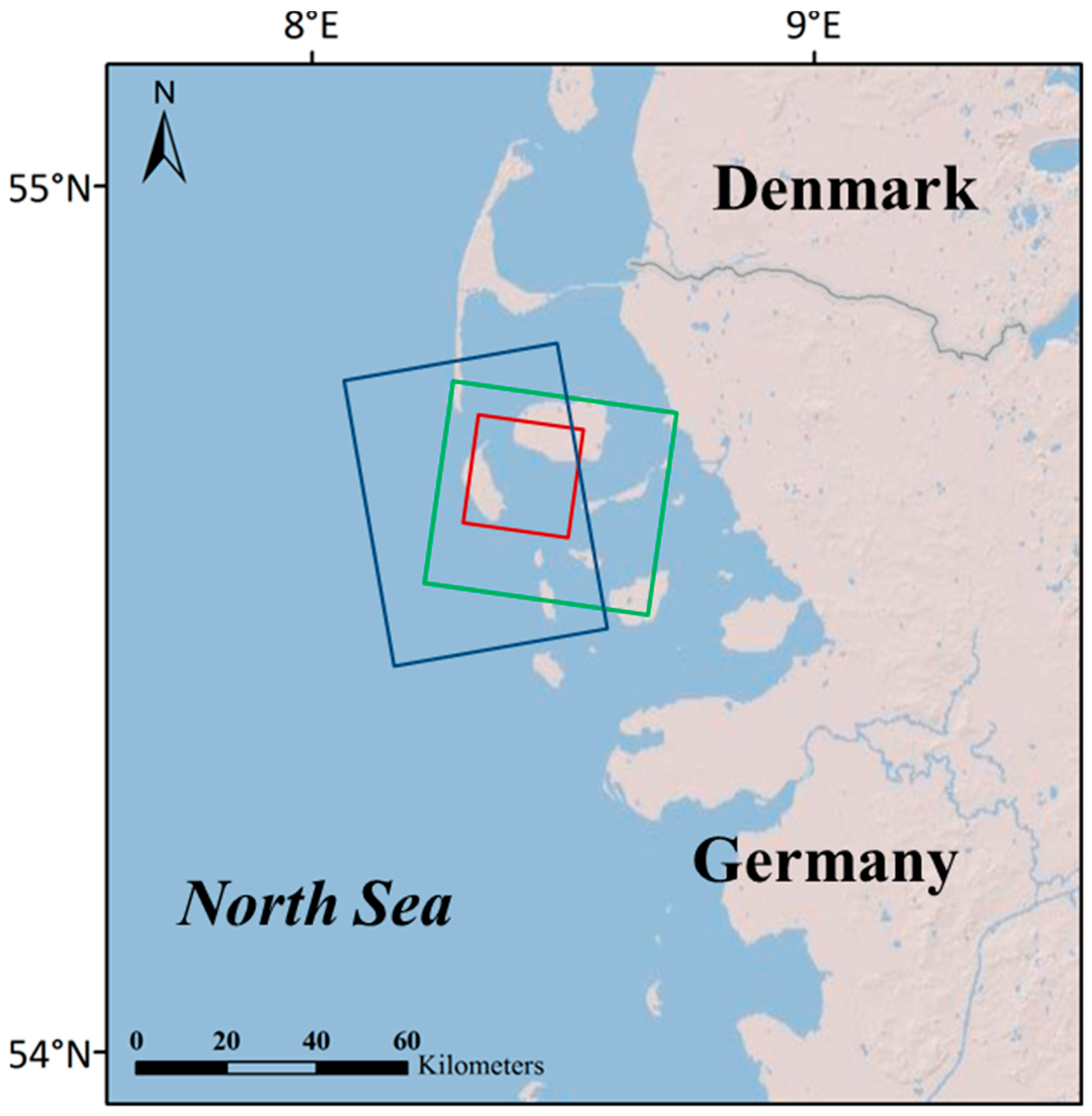
Figure 2.
Synthetic Aperture Radar (SAR) images of the test site “Amrum” in VV-polarization. (a) TSX data acquired on 20 June 2016, at 05:50 UTC © DLR; (b) RS2 data on 24 December 2015, at 05:43 UTC, Radarsat-2 data and products © MacDonald, Dettwiler and Associates Ltd. 2015 – All Rights Reserved; (c) AL2 data on 29 February 2016, at 23:10 UTC © JAXA. The red rectangle marks the area of interest (8.97 km × 8.31 km); the red star marks the location of tide gauge “Wittdün”.
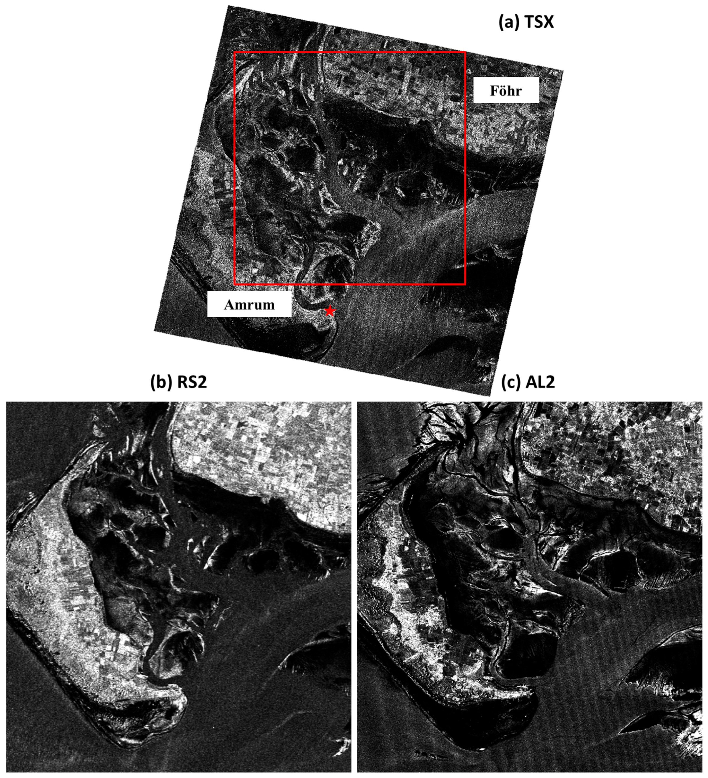
Figure 3.
Left: TSX VV-pol SAR image of 20 June 2016. The red lines denote the spatial extent of bivalve beds, as obtained from field excursions, the yellow line is a transect through bare flats and tidal creeks, but also through bivalve beds; upper right: map showing the TSX SAR image location; lower right: photograph (S. Melchionna) of oyster beds showing the typical structures with elevated patches of oysters, water puddles, and sediments.
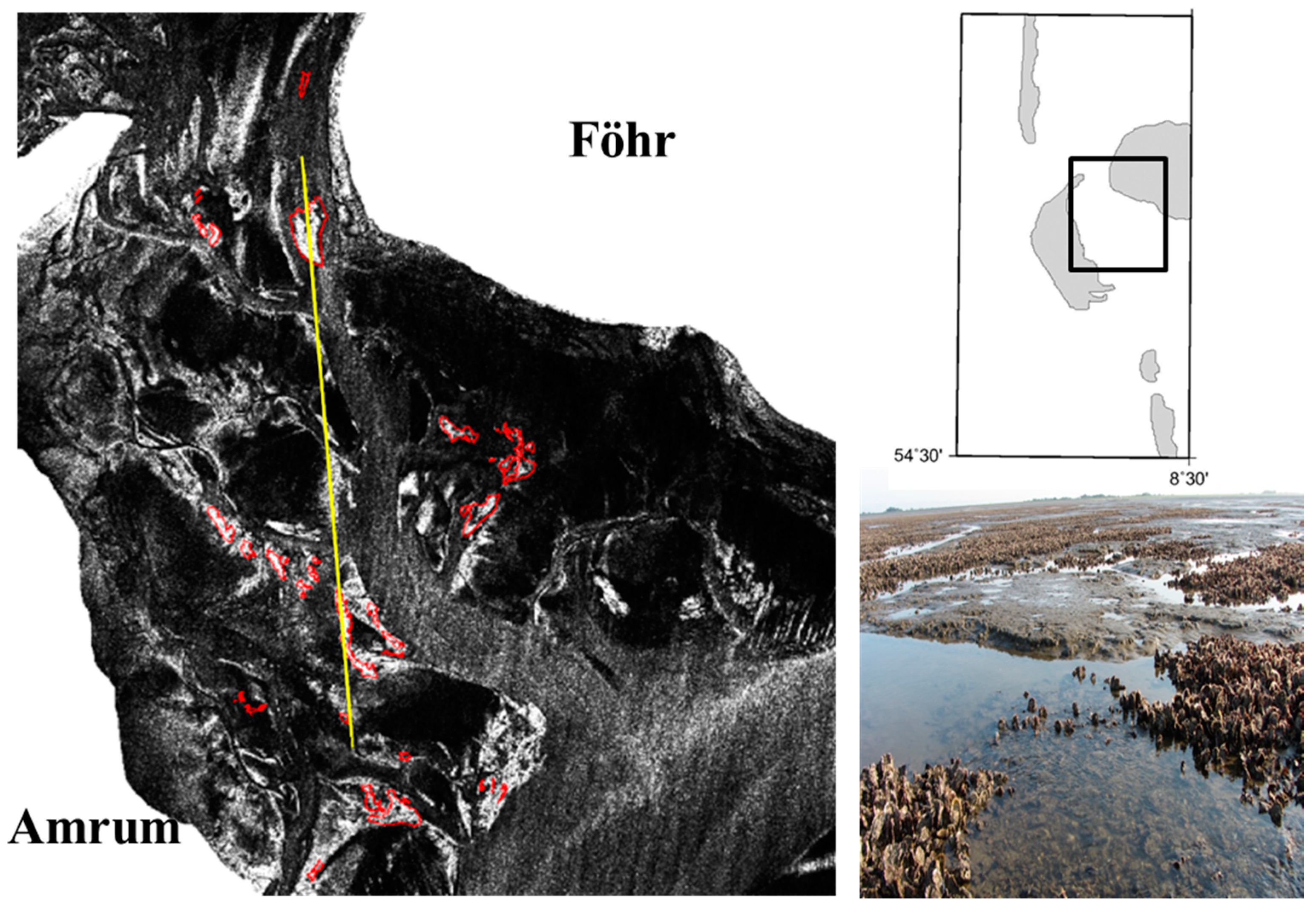
Figure 4.
Comparisons of the normalized radar cross section (NRCS) (solid lines) and noise equivalent sigma zero (NESZ) (dashed-dotted lines) along the yellow transect line marked in Figure 3. Blue: TSX; red: RS2; green: AL2. The dashed-dotted lines were raised by 2 dB to better demonstrate where the SAR data’s SNR was better than 2 dB. The thick horizontal bars on the abscissae indicate the locations of bivalve beds found in field excursions in 2015.
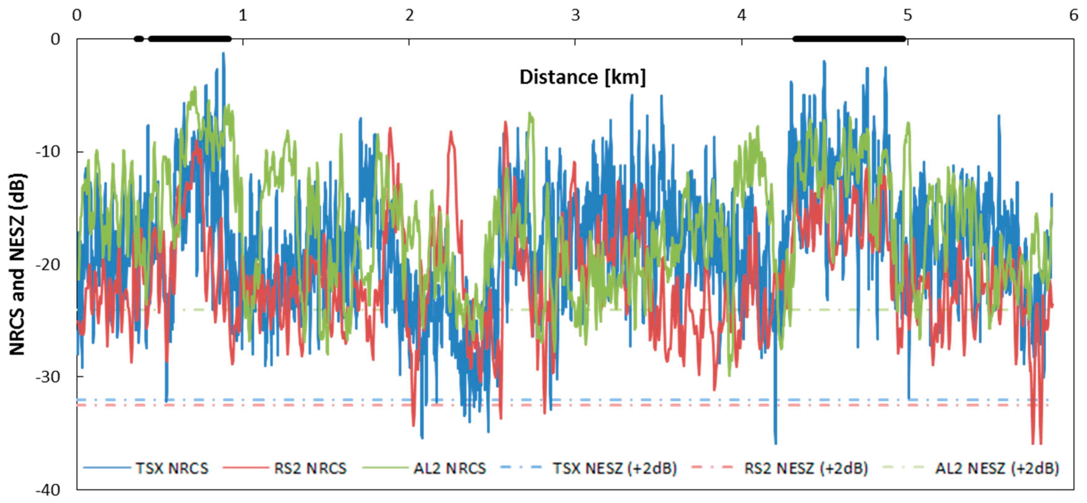
Figure 5.
The four Kennaugh elements derived from dual-copol SAR data. Columns (from left to right): K0 (sum of HH and VV intensities), K3 (difference between even- and odd-bounce scattering), K4 (difference of HH and VV intensities), K7 (phase shift between even- and odd-bounce scattering); rows (from top to bottom): (a) TSX (20 June 2016), (b) RS2 (24 December 2015), (c) AL2 (29 February 2016).
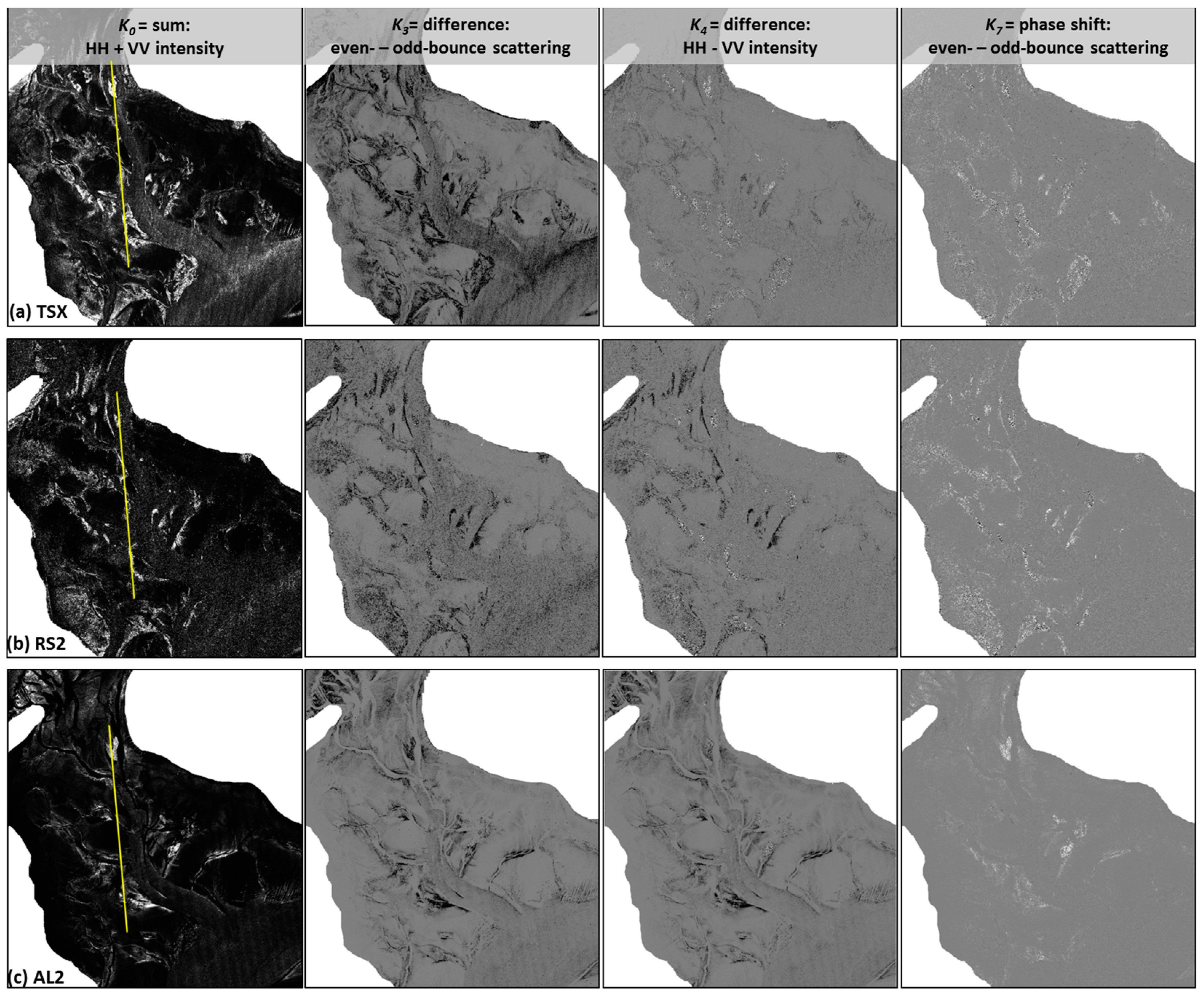
Figure 6.
Profiles along the transect line included in Figure 3 and Figure 5 from north (N) to south (S). Blue: running mean; red: running standard deviation; green: difference of both; each calculated for K3 (left column) and K7 (right column). Upper row: X-band; middle row: C-band; lower row: L-band. The thick horizontal bars on the top and bottom frames indicate the locations of bivalve beds found in field excursions in 2015.

Figure 7.
Difference D3 of the running mean and standard deviation of Kennaugh element K3 derived from (a) TSX X-band data, (b) RS2 C-band data, (c) AL2 L-band data, each calculated for a moving window of size 11 pixels × 11 pixels.
Figure 7.
Difference D3 of the running mean and standard deviation of Kennaugh element K3 derived from (a) TSX X-band data, (b) RS2 C-band data, (c) AL2 L-band data, each calculated for a moving window of size 11 pixels × 11 pixels.

Figure 8.
Same as Figure 7, but for the Difference D7.
Figure 8.
Same as Figure 7, but for the Difference D7.

Figure 9.
Product P of the absolute mean and standard deviation, each calculated for a running 11 pixels × 11 pixels window using (a) TSX X-band data [11]; (b) RS2 C-band data; (c) AL2 L-band data. The borders of bivalve beds found during field campaigns are inserted as red lines, and the map on the upper right shows the location of the area of interest.

Table 1.
SAR acquisition dates, times, sensors, modes, and environmental conditions during image acquisitions. Polarizations: dual-copol HH + VV (D), quad-pol HH + HV + VH + VV (Q).
Table 1.
SAR acquisition dates, times, sensors, modes, and environmental conditions during image acquisitions. Polarizations: dual-copol HH + VV (D), quad-pol HH + HV + VH + VV (Q).
| Date/Time [UTC] | Sensor/Band | Polarization/Incidence Angle | Water Level [cm] | Time (UTC)/Water Level [cm] at Low Tide |
|---|---|---|---|---|
| 20 June 2016/05:50 | TSX/X Band | D/31.4° | −160 | 06:22/−171 |
| 24 December 2015/05:43 | RS2/C Band | Q/36.3° | −94 | 05:25/−103 |
| 29 February 2016/23:10 | AL2/L Band | Q/35.3° | −171 | 23:46/−176 |
Table 2.
Detection accuracies of indicators for bivalve beds at all wavelengths (X-, C-, and L-band).
Table 2.
Detection accuracies of indicators for bivalve beds at all wavelengths (X-, C-, and L-band).
| Indicator | Detection Accuracy (%) | ||
|---|---|---|---|
| TSX | RS2 | AL2 | |
| D3 | 88.87 | 86.35 | 84.70 |
| D7 | 85.13 | 83.72 | 81.02 |
| P | 87.72 | 85.59 | 84.72 |
© 2017 by the authors. Licensee MDPI, Basel, Switzerland. This article is an open access article distributed under the terms and conditions of the Creative Commons Attribution (CC BY) license (http://creativecommons.org/licenses/by/4.0/).
Share and Cite
MDPI and ACS Style
Wang, W.; Gade, M.; Yang, X. Detection of Bivalve Beds on Exposed Intertidal Flats Using Polarimetric SAR Indicators. Remote Sens. 2017, 9, 1047. https://doi.org/10.3390/rs9101047
AMA Style
Wang W, Gade M, Yang X. Detection of Bivalve Beds on Exposed Intertidal Flats Using Polarimetric SAR Indicators. Remote Sensing. 2017; 9(10):1047. https://doi.org/10.3390/rs9101047
Chicago/Turabian StyleWang, Wensheng, Martin Gade, and Xiaofeng Yang. 2017. "Detection of Bivalve Beds on Exposed Intertidal Flats Using Polarimetric SAR Indicators" Remote Sensing 9, no. 10: 1047. https://doi.org/10.3390/rs9101047
Note that from the first issue of 2016, this journal uses article numbers instead of page numbers. See further details here.