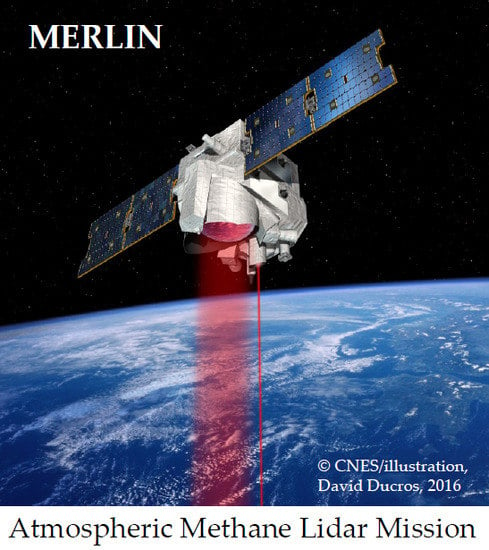
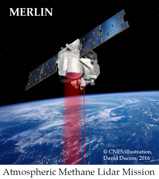
MERLIN: A French-German Space Lidar Mission Dedicated to Atmospheric Methane

 , , , , , , ,
  , ,
, ,
Abstract
:
1. Introduction
2. Mission Objectives
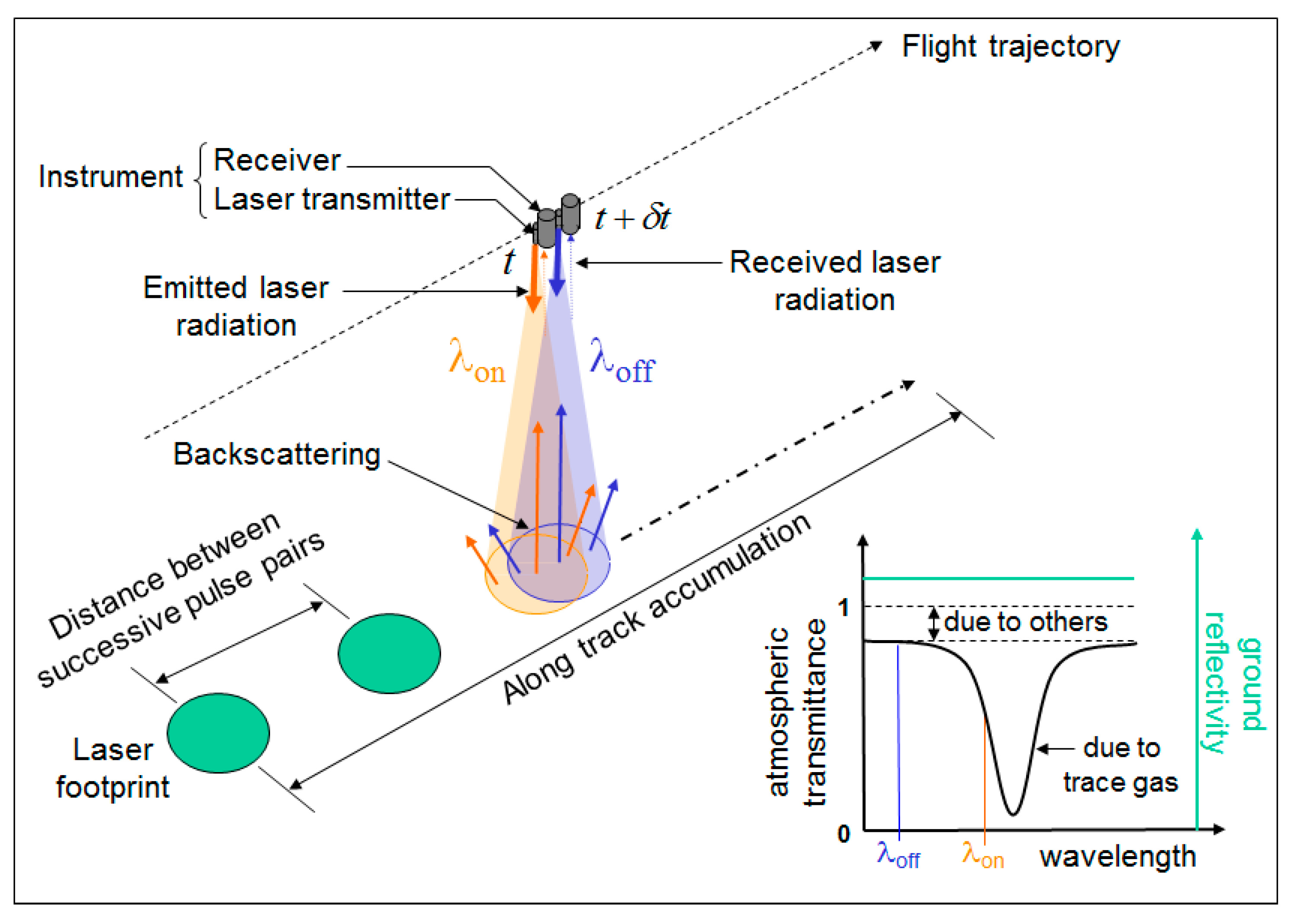
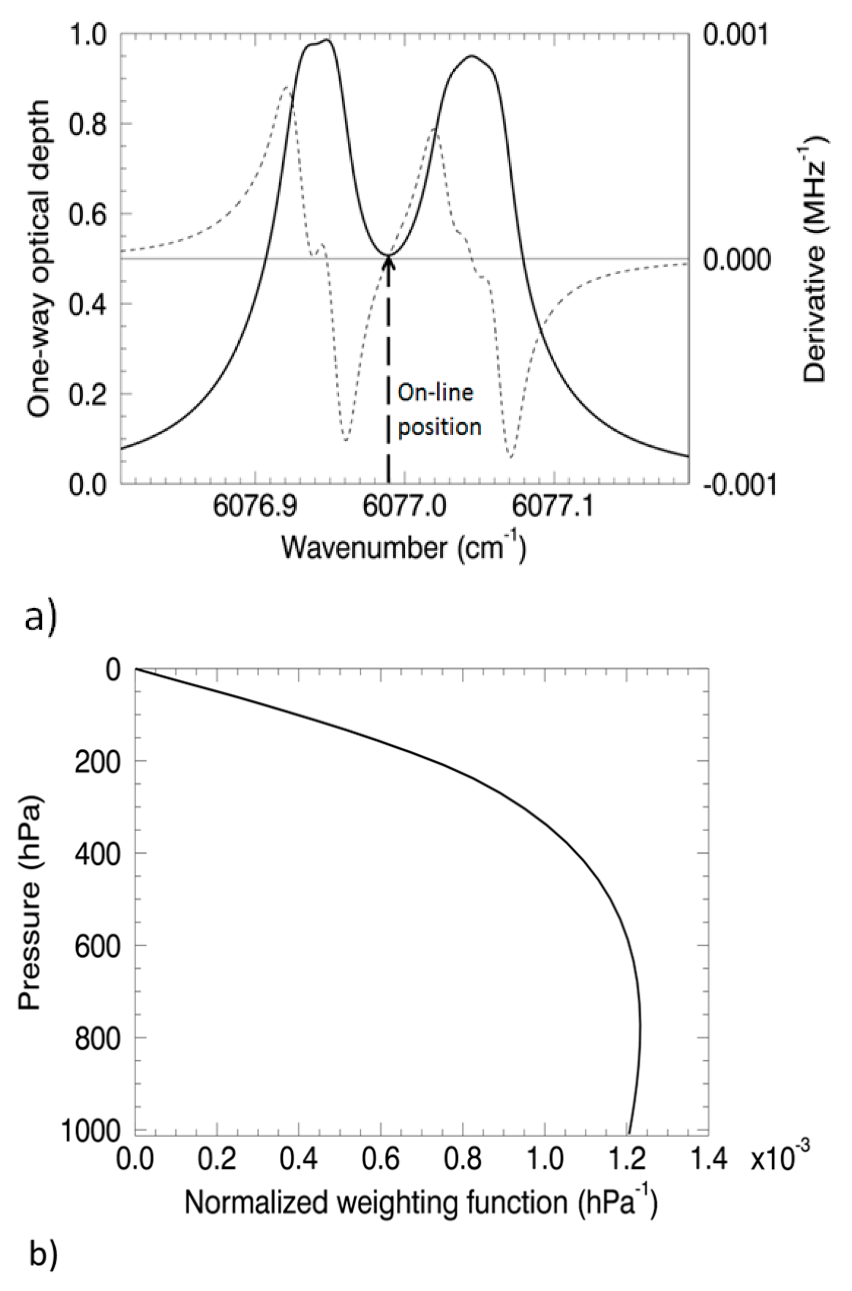
3. Methodology
4. Mission Elements
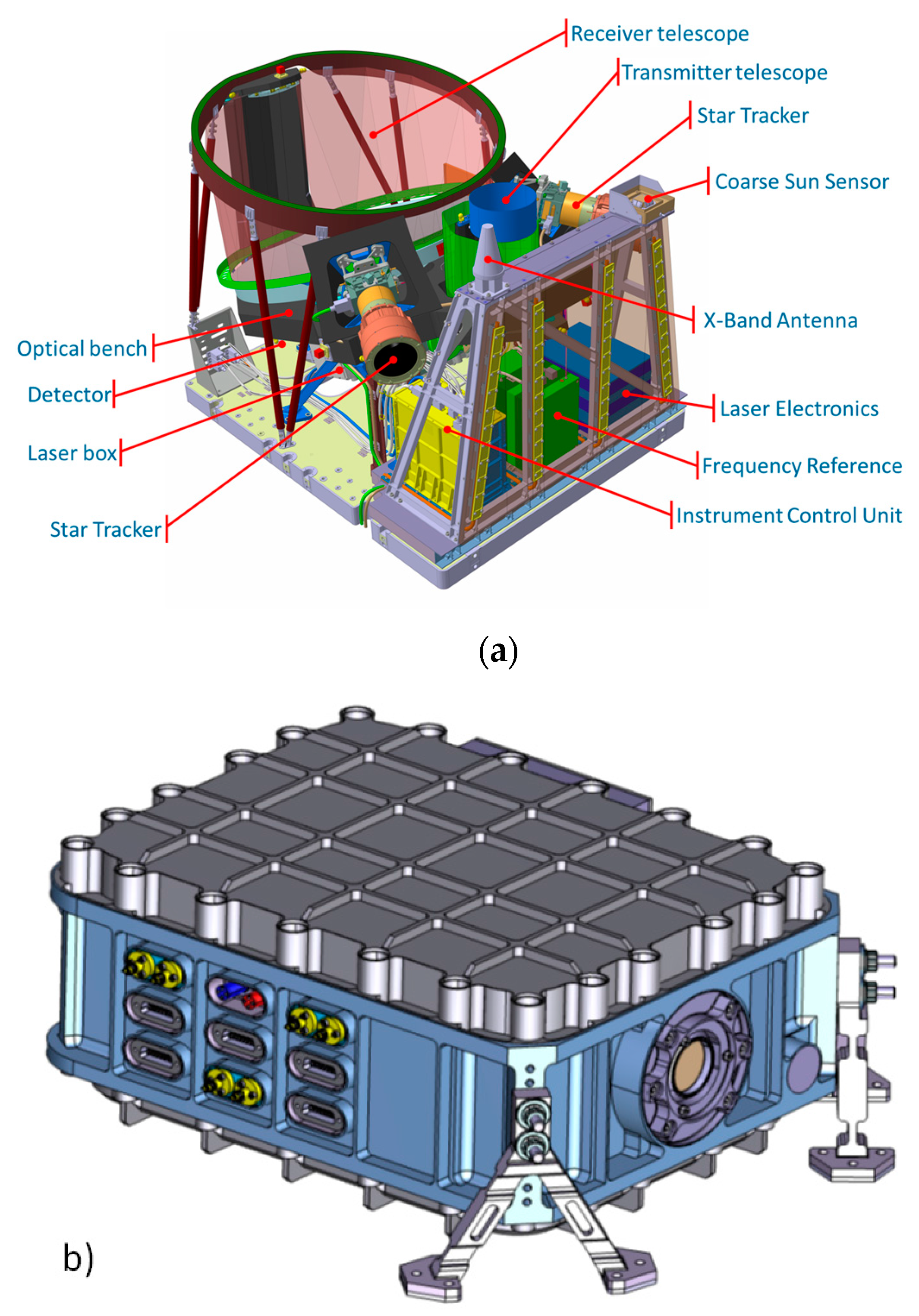
4.1. Space Segment
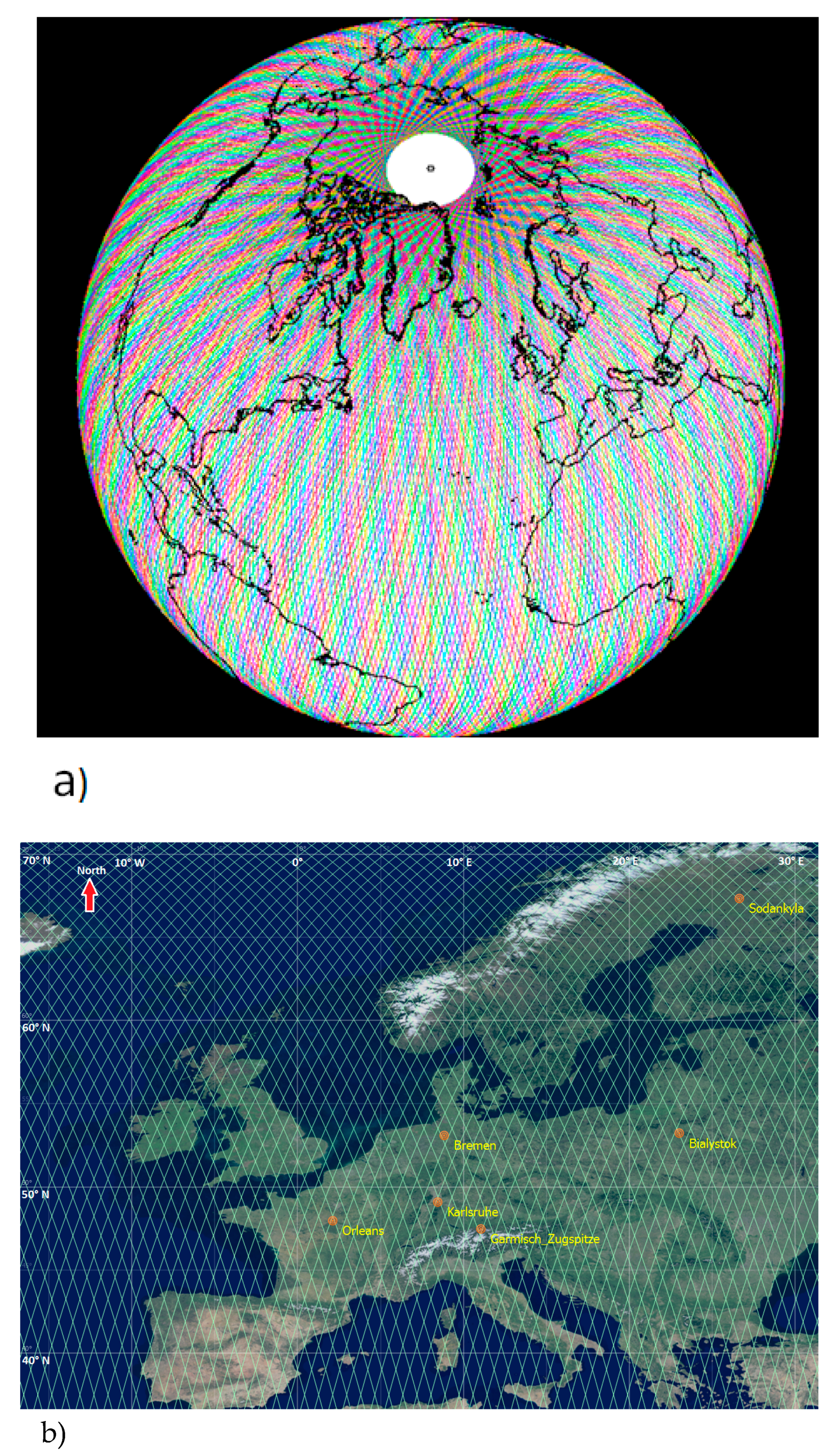
4.2. Mission Orbit
4.3. Data and Products
4.4. Validation
5. Performance
5.1. XCH4 Error Budget
5.2. Random and Systematic Error Scenarios
5.3. Expected Uncertainty Reductions on Surface Emission
6. Conclusions
Acknowledgments
Author Contributions
Conflicts of Interest
References
- Hartmann, D.L.; Klein Tank, A.M.G.; Rusticucci, M.; Alexander, L.V.; Brönnimann, S.; Charabi, Y.; Dentener, F.J.; Dlugokencky, E.J.; Easterling, D.R.; Kaplan, A.; et al. Observations: Atmosphere and surface. In Climate Change 2013: The Physical Science Basis. Contribution of Working Group I to the Fifth Assessment Report of the Intergovernmental Panel on Climate Change; Cambridge University Press: Cambridge, UK; New York, NY, USA, 2013. [Google Scholar]
- Saunois, M.; Bousquet, P.; Poulter, B.; Peregon, A.; Ciais, P.; Canadell, J.G.; Dlugokencky, E.J.; Etiope, G.; Bastviken, D.; Houweling, S.; et al. The global methane budget 2000–2012. Earth Syst. Sci. Data 2016, 8, 697–751. [Google Scholar] [CrossRef]
- WMO. World Meteorological Organisation, World Data Centre for Greenhouse Gases (WDCGG), Japan Meteorological Agency. Available online: http://ds.data.jma.go.jp/gmd/wdcgg/introduction.html (accessed on 31 March 2017).
- Blake, D.R.; Mayer, E.W.; Tyler, S.C.; Makide, Y.; Montague, D.C.; Rowland, F.S. Global increase in atmospheric methane concentrations between 1978 and 1980. Geophys. Res. Lett. 1982, 9, 477–480. [Google Scholar] [CrossRef]
- Sweeney, C.; Karion, A.; Wolter, S.; Newberger, T.; Guenther, D.; Higgs, J.A.; Andrews, A.E.; Lang, P.M.; Neff, D.; Dlugokencky, E.; et al. Seasonal climatology of CO2 across north america from aircraft measurements in the noaa/esrl global greenhouse gas reference network. J. Geophys. Res. Atmos. 2015, 120, 5155–5190. [Google Scholar] [CrossRef]
- Brenninkmeijer, C.A.M.; Crutzen, P.; Boumard, F.; Dauer, T.; Dix, B.; Ebinghaus, R.; Filippi, D.; Fischer, H.; Franke, H.; Frieβ, U.; et al. Civil aircraft for the regular investigation of the atmosphere based on an instrumented container: The new caribic system. Atmos. Chem. Phys. 2007, 7, 4953–4976. [Google Scholar] [CrossRef] [Green Version]
- Schuck, T.J.; Ishijima, K.; Patra, P.K.; Baker, A.K.; Machida, T.; Matsueda, H.; Sawa, Y.; Umezawa, T.; Brenninkmeijer, C.A.M.; Lelieveld, J. Distribution of methane in the tropical upper troposphere measured by caribic and contrail aircraft. J. Geophys. Res. Atmos. 2012, 117, D19304. [Google Scholar] [CrossRef]
- Chang, R.Y.W.; Miller, C.E.; Dinardo, S.J.; Karion, A.; Sweeney, C.; Daube, B.C.; Henderson, J.M.; Mountain, M.E.; Eluszkiewicz, J.; Miller, J.B.; et al. Methane emissions from alaska in 2012 from carve airborne observations. Proc. Natl. Acad. Sci. USA 2014, 111, 16694–16699. [Google Scholar] [CrossRef] [PubMed]
- Paris, J.D.; Stohl, A.; Ciais, P.; Nédélec, P.; Belan, B.D.; Arshinov, M.Y.; Ramonet, M. Source-receptor relationships for airborne measurements of CO2, CO and O3 above siberia: A cluster-based approach. Atmos. Chem. Phys. 2010, 10, 1671–1687. [Google Scholar] [CrossRef] [Green Version]
- Wofsy, S.; The HIPPO Science Team; Cooperating Modellers and Satellite Teams. Hiaper pole-to-pole observations (hippo): Fine grained, global scale measurements of climatically important atmospheric gases and aerosols. Phil. Trans. R. Soc. A 2011, 369, 2073–2086. [Google Scholar] [CrossRef] [PubMed]
- Karion, A.; Sweeney, C.; Tans, P.; Newberger, T. Aircore: An innovative atmospheric sampling system. J. Atmos. Ocean. Technol. 2010, 27, 1839–1853. [Google Scholar] [CrossRef]
- Wunch, D.; Toon, G.C.; Blavier, J.-F.L.; Washenfelder, R.A.; Notholt, J.; Connor, B.J.; Griffith, D.W.T.; Sherlock, V.; Wennberg, P.O. The total carbon column observing network. Phil. Trans. R. Soc. A 2011, 369. [Google Scholar] [CrossRef] [PubMed]
- Gerilowski, K.; Tretner, A.; Krings, T.; Buchwitz, M.; Bertagnolio, P.P.; Belemezov, F.; Erzinger, J.; Burrows, J.P.; Bovensmann, H. Mamap—A new spectrometer system for column-averaged methane and carbon dioxide observations from aircraft: Instrument description and performance analysis. Atmos. Meas. Tech. 2011, 4, 215–243. [Google Scholar] [CrossRef]
- Krings, T.; Gerilowski, K.; Buchwitz, M.; Hartmann, J.; Sachs, T.; Erzinger, J.; Burrows, J.P.; Bovensmann, H. Quantification of methane emission rates from coal mine ventilation shafts using airborne remote sensing data. Atmos. Meas. Tech. 2013, 6, 151–166. [Google Scholar] [CrossRef] [Green Version]
- Krautwurst, S.; Gerilowski, K.; Jonsson, H.H.; Thompson, D.R.; Kolyer, R.W.; Thorpe, A.K.; Horstjann, M.; Eastwood, M.; Leifer, I.; Vigil, S.; et al. Methane emissions from a californian landfill, determined from airborne remote sensing and in-situ measurements. Atmos. Meas. Tech. 2017, 10, 3429–3452. [Google Scholar] [CrossRef]
- Bousquet, P.; Ciais, P.; Miller, J.B.; Dlugokencky, E.J.; Hauglustaine, D.A.; Prigent, C.; Van der Werf, G.R.; Peylin, P.; Brunke, E.G.; Carouge, C.; et al. Contribution of anthropogenic and natural sources to atmospheric methane variability. Nature 2006, 443, 439–443. [Google Scholar] [CrossRef] [PubMed]
- Houweling, S.; Kaminski, T.; Dentener, F.; Lelieveld, J.; Heimann, M. Inverse modeling of methane sources and sinks using the adjoint of a global transport model. J. Geophys. Res. Atmos. 1999, 104, 26137–26160. [Google Scholar] [CrossRef]
- INFLUX. Indianapolis Flux Experiment. Available online: http://sites.psu.edu/influx/ (accessed on 25 August 2017).
- Lamb, B.K.; Cambaliza, M.O.L.; Davis, K.J.; Edburg, S.L.; Ferrara, T.W.; Floerchinger, C.; Heimburger, A.M.F.; Herndon, S.; Lauvaux, T.; Lavoie, T.; et al. Direct and indirect measurements and modeling of methane emissions in Indianapolis, Indiana. Environ. Sci. Technol. 2016, 50, 8910–8917. [Google Scholar] [CrossRef] [PubMed]
- Viatte, C.; Lauvaux, T.; Hedelius, J.K.; Parker, H.; Chen, J.; Jones, T.; Franklin, J.E.; Deng, A.J.; Gaudet, B.; Verhulst, K.; et al. Methane emissions from dairies in the los angeles basin. Atmos. Chem. Phys. 2017, 17, 7509–7528. [Google Scholar] [CrossRef]
- Wong, C.K.; Pongetti, T.J.; Oda, T.; Rao, P.; Gurney, K.R.; Newman, S.; Duren, R.M.; Miller, C.E.; Yung, Y.L.; Sander, S.P. Monthly trends of methane emissions in los angeles from 2011 to 2015 inferred by clars-fts observations. Atmos. Chem. Phys. 2016, 16, 13121–13130. [Google Scholar] [CrossRef]
- Locatelli, R.; Bousquet, P.; Saunois, M.; Chevallier, F.; Cressot, C. Sensitivity of the recent methane budget to lmdz sub-grid-scale physical parameterizations. Atmos. Chem. Phys. 2015, 15, 9765–9780. [Google Scholar] [CrossRef]
- Patra, P.K.; Houweling, S.; Krol, M.; Bousquet, P.; Belikov, D.; Bergmann, D.; Bian, H.; Cameron-Smith, P.; Chipperfield, M.P.; Corbin, K.; et al. Transcom model simulations of ch4 and related species: Linking transport, surface flux and chemical loss with ch4 variability in the troposphere and lower stratosphere. Atmos. Chem. Phys. 2011, 11, 12813–12837. [Google Scholar] [CrossRef] [Green Version]
- Dlugokencky, E.J.; Bruhwiler, L.; White, J.W.C.; Emmons, L.K.; Novelli, P.C.; Montzka, S.A.; Masarie, K.A.; Lang, P.M.; Crotwell, A.M.; Miller, J.B.; et al. Observational constraints on recent increases in the atmospheric ch burden. Geophys. Res. Lett. 2009, 36, L18803. [Google Scholar] [CrossRef]
- Miller, S.M.; Wofsy, S.C.; Michalak, A.M.; Kort, E.A.; Andrews, A.E.; Biraud, S.C.; Dlugokencky, E.J.; Eluszkiewicz, J.; Fischer, M.L.; Janssens-Maenhout, G.; et al. Anthropogenic emissions of methane in the united states. Proc. Natl. Acad. Sci. USA 2013, 110, 20018–20022. [Google Scholar] [CrossRef] [PubMed]
- Delahaye, T.; Reed, Z.; Maxwell, S.; Hodges, J.T.; Sung, K.; Brown, L.; Benner, C.; Devi, V.M.; Warneke, T.; Spietz, P.; et al. Precise methane absorption measurements in the 1.64 µm spectral region for the merlin mission. J. Geophys. Res. Atmos. 2016, 121, 7360–7370. [Google Scholar] [CrossRef] [PubMed]
- Bousquet, P.; Ehret, G.; Group, M.S.A. The MERLIN Science Plan; CNES: Toulouse, France, 2015; Available online: https://files.lsce.ipsl.fr/public.php?service=files&t=9f79de7f3eabfe3655393efebef43377 (accessed on 25 August 2017).
- GAW Report #213. In Proceedings of the 17th WMO/IAEA Meeting on Carbon Dioxide, Other Greenhouse Gases and Related Tracers Measurement Techniques (GGMT-2013), Beijing, China, 10–13 June 2013; World Meteorological Organization: Geneva, Switzerland, 2014.
- Bovensmann, H.; Burrows, J.P.; Buchwitz, M.; Frerick, J.; Noël, S.; Rozanov, V.V.; Chance, K.V.; Goede, A.P.H. Sciamachy: Mission objectives and measurement modes. J. Atmos. Sci. 1999, 56, 127–150. [Google Scholar] [CrossRef]
- Buchwitz, M.; De Beek, R.; Noel, S.; Burrows, J.P.; Bovensmann, H.; Schneising, O.; Khlystova, I.; Bruns, M.; Bremer, H.; Bergamaschi, P.; et al. Atmospheric carbon gases retrieved from sciamachy by wfm-doas: Version 0.5 co and ch4 and impact of calibration improvements on CO2 retrieval. Atmos. Chem. Phys. 2006, 6, 2727–2751. [Google Scholar] [CrossRef]
- Buchwitz, M.; Reuter, M.; Schneising, O.; Boesch, H.; Guerlet, S.; Dils, B.; Aben, I.; Armante, R.; Bergamaschi, P.; Blumenstock, T.; et al. The greenhouse gas climate change initiative (ghg-cci): Comparison and quality assessment of near-surface-sensitive satellite-derived CO2 and CH4 global data sets. Remote Sens. Environ. 2015, 162, 344–362. [Google Scholar] [CrossRef]
- Burrows, J.P.; Hölzle, E.; Goede, A.P.H.; Visser, H.; Fricke, W. Sciamachy—Scanning imaging absorption spectrometer for atmospheric chartography. Acta Astronaut. 1995, 35, 445–451. [Google Scholar] [CrossRef]
- Dils, B.; De Mazière, M.; Müller, J.F.; Blumenstock, T.; Buchwitz, M.; De Beek, R.; Demoulin, P.; Duchatelet, P.; Fast, H.; Frankenberg, C.; et al. Comparisons between sciamachy and ground-based ftir data for total columns of CO, CH4, CO2 and N2O. Atmos. Chem. Phys. 2006, 6, 1953–1976. [Google Scholar] [CrossRef]
- Frankenberg, C.; Aben, I.; Bergamaschi, P.; Dlugokencky, E.J.; Van Hees, R.; Houweling, S.; Van der Meer, P.; Snel, R.; Tol, P. Global column-averaged methane mixing ratios from 2003 to 2009 as derived from sciamachy: Trends and variability. J. Geophys. Res. Atmos. 2011, 116, D04302. [Google Scholar] [CrossRef]
- Butz, A.; Guerlet, S.; Hasekamp, O.; Schepers, D.; Galli, A.; Aben, I.; Frankenberg, C.; Hartmann, J.M.; Tran, H.; Kuze, A.; et al. Toward accurate CO(2) and CH(4) observations from gosat. Geophys. Res. Lett. 2011, 38, L14812. [Google Scholar] [CrossRef]
- Morino, I.; Uchino, O.; Inoue, M.; Yoshida, Y.; Yokota, T.; Wennberg, P.O.; Toon, G.C.; Wunch, D.; Roehl, C.M.; Notholt, J.; et al. Preliminary validation of column-averaged volume mixing ratios of carbon dioxide and methane retrieved from gosat short-wavelength infrared spectra. Atmos. Meas. Tech. 2011, 4, 1061–1076. [Google Scholar] [CrossRef]
- Bergamaschi, P.; Frankenberg, C.; Meirink, J.F.; Krol, M.; Dentener, F.; Wagner, T.; Platt, U.; Kaplan, J.O.; Koerner, S.; Heimann, M.; et al. Satellite chartography of atmospheric methane from sciamachyon board envisat: 2. Evaluation based on inverse model simulations. J. Geophys. Res. Atmos. 2007, 112, D2. [Google Scholar] [CrossRef]
- Bergamaschi, P.; Frankenberg, C.; Meirink, J.F.; Krol, M.; Villani, M.G.; Houweling, S.; Dentener, F.; Dlugokencky, E.J.; Miller, J.B.; Gatti, L.V.; et al. Inverse modeling of global and regional CH4 emissions using sciamachy satellite retrievals. J. Geophys. Res. Atmos. 2009, 114, D22. [Google Scholar] [CrossRef]
- Bergamaschi, P.; Houweling, S.; Segers, A.; Krol, M.; Frankenberg, C.; Scheepmaker, R.A.; Dlugokencky, E.; Wofsy, S.C.; Kort, E.A.; Sweeney, C.; et al. Atmospheric CH4 in the first decade of the 21st century: Inverse modeling analysis using sciamachy satellite retrievals and noaa surface measurements. J. Geophys. Res. Atmos. 2013, 118, 7350–7369. [Google Scholar] [CrossRef]
- Houweling, S.; Krol, M.; Bergamaschi, P.; Frankenberg, C.; Dlugokencky, E.J.; Morino, I.; Notholt, J.; Sherlock, V.; Wunch, D.; Beck, V.; et al. A multi-year methane inversion using sciamachy, accounting for systematic errors using tccon measurements. Atmos. Chem. Phys. 2014, 14, 10961–10962. [Google Scholar] [CrossRef]
- Meirink, J.F.; Bergamaschi, P.; Frankenberg, C.; d’Amelio, M.T.S.; Dlugokencky, E.J.; Gatti, L.V.; Houweling, S.; Miller, J.B.; Rockmann, T.; Villani, M.G.; et al. Four-dimensional variational data assimilation for inverse modeling of atmospheric methane emissions: Analysis of sciamachy observations. J. Geophys. Res. Atmos. 2008, 113, D17. [Google Scholar] [CrossRef]
- Cressot, C.; Chevallier, F.; Bousquet, P.; Crevoisier, C.; Dlugokencky, E.J.; Fortems-Cheiney, A.; Frankenberg, C.; Parker, R.; Pison, I.; Scheepmaker, R.A.; et al. On the consistency between global and regional methane emissions inferred from sciamachy, tanso-fts, iasi and surface measurements. Atmos. Chem. Phys. 2014, 14, 577–592. [Google Scholar] [CrossRef]
- Monteil, G.; Houweling, S.; Butz, A.; Guerlet, S.; Schepers, D.; Hasekamp, O.; Frankenberg, C.; Scheepmaker, R.; Aben, I.; Röckmann, T. Comparison of ch4 inversions based on 15 months of gosat and sciamachy observations. J. Geophys. Res. Atmos. 2013, 118, 11807–11823. [Google Scholar] [CrossRef]
- Kort, E.A.; Frankenberg, C.; Costigan, K.R.; Lindenmaier, R.; Dubey, M.K.; Wunch, D. Four corners: The largest us methane anomaly viewed from space. Geophys. Res. Lett. 2014, 41, 6898–6903. [Google Scholar] [CrossRef]
- Buchwitz, M.; Schneising, O.; Reuter, M.; Heymann, J.; Krautwurst, S.; Bovensmann, H.; Burrows, J.P.; Boesch, H.; Parker, R.J.; Somkuti, P.; et al. Satellite-derived methane hotspot emission estimates using a fast data-driven method. Atmos. Chem. Phys. 2017, 17, 5751–5774. [Google Scholar] [CrossRef]
- Crevoisier, C.; Nobileau, D.; Fiore, A.M.; Armante, R.; Chedin, A.; Scott, N.A. Tropospheric methane in the tropics—First year from iasi hyperspectral infrared observations. Atmos. Chem. Phys. 2009, 9, 6337–6350. [Google Scholar] [CrossRef]
- Alexe, M.; Bergamaschi, P.; Segers, A.; Detmers, R.; Butz, A.; Hasekamp, O.; Guerlet, S.; Parker, R.; Boesch, H.; Frankenberg, C.; et al. Inverse modelling of CH4 emissions for 2010–2011 using different satellite retrieval products from gosat and sciamachy. Atmos. Chem. Phys. 2015, 15, 113–133. [Google Scholar] [CrossRef] [Green Version]
- Buchwitz, M.; Dils, B.; Boesch, H.; Crevoisier, C.; Detmers, R.; Frankenberg, C.; Hasekamp, O.; Hewson, W.; Laeng, A.; Noel, S.; et al. Product Validation and Intercomparison Report (PVIR); Version 4.0, CRDP#3; From ESA Climate Change Initiative (CCI); European Space Agency: Paris, France, 2016; Available online: http://www.esa-ghg-cci.org/?q=node/95 (accessed on 25 August 2017).
- Hu, H.; Hasekamp, O.; Butz, A.; Galli, A.; Landgraf, J.; Aan de Brugh, J.; Borsdorff, T.; Scheepmaker, R.; Aben, I. The operational methane retrieval algorithm for tropomi. Atmos. Meas. Tech. 2016, 9, 5423–5440. [Google Scholar] [CrossRef]
- Glumb, R.; Davis, G.; Lietzke, C. The tanso-fts-2 instrument for the gosat-2 greenhouse gas monitoring mission. In Proceedings of the 2014 IEEE International Geoscience and Remote Sensing Symposium (IGARSS), Quebec City, QC, Canada, 6 November 2014; pp. 1238–1240. [Google Scholar]
- O’Brien, D.M.; Polonsky, I.N.; Utembe, S.R.; Rayner, P.J. Potential of a geostationary geocarb mission to estimate surface emissions of CO2, CH4 and CO in a polluted urban environment: Case study shanghai. Atmos. Meas. Tech. 2016, 9, 4633–4654. [Google Scholar]
- Crevoisier, C.; Clerbaux, C.; Guidard, V.; Phulpin, T.; Armante, R.; Barret, B.; Camy-Peyret, C.; Chaboureau, J.P.; Coheur, P.F.; Crépeau, L.; et al. Towards iasi-new generation (iasi-ng): Impact of improved spectral resolution and radiometric noise on the retrieval of thermodynamic, chemistry and climate variables. Atmos. Meas. Tech. 2014, 7, 4367–4385. [Google Scholar] [CrossRef] [Green Version]
- Ehret, G.; Kiemle, C.; Wirth, M.; Amediek, A.; Fix, A.; Houweling, S. Space-borne remote sensing of CO2, CH4, and N2O by integrated path differential absorption Lidar: A sensitivity analysis. Appl. Phys. B Lasers Opt. 2008, 90, 593–608. [Google Scholar] [CrossRef] [Green Version]
- Flamant, P.; Ehret, G.; Millet, B.; Alpers, M. Merlin: A French-German mission addressing methane monitoring by Lidar from space. In Proceedings of the 26th International Laser Radar Conference (ILRC), Porto Heli, Greece, 26–29 June 2012. [Google Scholar]
- Kiemle, C.; Quatrevalet, M.; Ehret, G.; Amediek, A.; Fix, A.; Wirth, M. Sensitivity studies for a space-based methane Lidar mission. Atmos. Meas. Tech. 2011, 4, 2195–2211. [Google Scholar] [CrossRef] [Green Version]
- Pierangelo, C.; Millet, B.; Esteve, F.; Alpers, M.; Ehret, G.; Flamant, P.H.; Berthier, S.; Gibert, F.; Chomette, O.; Edouart, D.; et al. Merlin (methane remote sensing Lidar mission): An overview. In Proceedings of the 27th International Laser Radar Conference (ILRC), New York, NY, USA, 5–10 July 2015; EPJ Web of Conferences: Les Ulis, France, 2016; Volume 119. [Google Scholar]
- Abshire, J.B.; Riris, H.; Allan, G.R.; Weaver, C.J.; Mao, J.; Sun, X.; Hasselbrack, W.E.; Kawa, S.R.; Biraud, S. Pulsed airborne Lidar measurements of atmospheric CO2 column absorption. Tellus B 2010, 62, 770–783. [Google Scholar] [CrossRef]
- Amediek, A.; Fix, A.; Wirth, M.; Ehret, G. Development of an opo system at 1.57 μm for integrated path dial measurement of atmospheric carbon dioxide. Appl. Phys. B 2008, 92, 295–302. [Google Scholar] [CrossRef] [Green Version]
- Gibert, F.; Flamant, P.H.; Bruneau, D.; Loth, C. Two-micrometer heterodyne differential absorption Lidar measurements of the atmospheric CO2 mixing ratio in the boundary layer. Appl. Opt. 2006, 45, 4448–4458. [Google Scholar] [CrossRef] [PubMed]
- Gibert, F.; Flamant, P.H.; Cuesta, J.; Bruneau, D. Vertical 2-μm heterodyne differential absorption Lidar measurements of mean CO2 mixing ratio in the troposphere. J. Atmos. Ocean. Technol. 2008, 25, 1477–1497. [Google Scholar] [CrossRef]
- Ishii, S.; Mizutani, K.; Fukuoka, H.; Ishikawa, T.; Philippe, B.; Iwai, H.; Aoki, T.; Itabe, T.; Sato, A.; Asai, K. Coherent 2 μm differential absorption and wind Lidar with conductively cooled laser and two-axis scanning device. Appl. Opt. 2010, 49, 1809–1817. [Google Scholar] [CrossRef] [PubMed]
- Koch, G.J.; Barnes, B.W.; Petros, M.; Beyon, J.Y.; Amzajerdian, F.; Yu, J.; Davis, R.E.; Ismail, S.; Vay, S.; Kavaya, M.J.; et al. Coherent differential absorption Lidar measurements of CO2. Appl. Opt. 2004, 43, 5092–5099. [Google Scholar] [CrossRef] [PubMed]
- Spiers, G.D.; Menzies, R.T.; Jacob, J.; Christensen, L.E.; Phillips, M.W.; Choi, Y.; Browell, E.V. Atmospheric CO2 measurements with a 2 μm airborne laser absorption spectrometer employing coherent detection. Appl. Opt. 2011, 50, 2098–2111. [Google Scholar] [CrossRef] [PubMed]
- NASA. Ascends: Mission Science Definition and Planning Workshop Report. Available online: https://cce.nasa.gov/ascends (accessed on 24 November 2016).
- Riris, H.; Numata, K.; Li, S.; Wu, S.; Ramanathan, A.; Dawsey, M.; Mao, J.; Kawa, R.; Abshire, J.B. Airborne measurements of atmospheric methane column abundance using a pulsed integrated-path differential absorption Lidar. Appl. Opt. 2012, 51, 8296–8305. [Google Scholar] [CrossRef] [PubMed]
- Amediek, A.; Ehret, G.; Fix, A.; Wirth, M.; Büdenbender, C.; Quatrevalet, M.; Kiemle, C.; Gerbig, C. Charm-F a new airborne integrated-path differential-absorption Lidar for carbon dioxide and methane observations: Measurement performance and quantification of strong point source emissions. Appl. Opt. 2017, 56, 5182–5197. [Google Scholar] [CrossRef]
- Wirth, M.; Fix, A.; Mahnke, P.; Schwarzer, H.; Schrandt, F.; Ehret, G. The airborne multi-wavelength water vapor differential absorption Lidar wales: System design and performance. Appl. Phys. B 2009, 96, 201. [Google Scholar] [CrossRef] [Green Version]
- Cosentino, A.; D’Ottavi, A.; Sapia, A.; Suetta, E. Spaceborne lasers development for aladin and atlid instruments. In Proceedings of the Geoscience and Remote Sensing Symposium (IGARSS), Munich, Germany, 22–27 July 2012; pp. 5673–5676. [Google Scholar] [CrossRef]
- Hunt, W.H.; Winker, D.M.; Vaughan, M.A.; Powell, K.A.; Lucker, P.L.; Weimer, C. Calipso Lidar description and performance assessment. J. Atmos. Ocean. Technol. 2009, 26, 1214–1228. [Google Scholar] [CrossRef]
- Winker, D.M.; Vaughan, M.A.; Omar, A.; Hu, Y.; Powell, K.A.; Liu, Z.; Hunt, W.H.; Young, S.A. Overview of the calipso mission and caliop data processing algorithms. J. Atmos. Ocean. Technol. 2009, 26, 2310–2323. [Google Scholar] [CrossRef]
- Strotkamp, M.; Elsen, F.; Löhring, J.; Traub, M.; Hoffmann, D. Two stage innoslab amplifier for energy scaling from 100 to >500 mj for future Lidar applications. Appl. Opt. 2017, 56, 2886–2892. [Google Scholar] [CrossRef] [PubMed]
- Frankenberg, C.; Meirink, J.F.; Bergamaschi, P.; Goede, A.P.H.; Heimann, M.; Korner, S.; Platt, U.; van Weele, M.; Wagner, T. Satellite chartography of atmospheric methane from sciamachy on board envisat: Analysis of the years 2003 and 2004. J. Geophys. Res. Atmos. 2006, 111, D07303. [Google Scholar] [CrossRef]
- Kuze, A.; Suto, H.; Shiomi, K.; Kawakami, S.; Tanaka, M.; Ueda, Y.; Deguchi, A.; Yoshida, J.; Yamamoto, Y.; Kataoka, F.; et al. Update on gosat tanso-fts performance, operations, and data products after more than 6 years in space. Atmos. Meas. Tech. 2016, 9, 2445–2461. [Google Scholar] [CrossRef]
- Butz, A.; Galli, A.; Hasekamp, O.; Landgraf, J.; Tol, P.; Aben, I. Tropomi aboard sentinel-5 precursor: Prospective performance of CH4 retrievals for aerosol and cirrus loaded atmospheres. Remote Sens. Environ. 2012, 120, 267–276. [Google Scholar] [CrossRef]
- ESA. Sentinel 5 ESA Webpage. Available online: https://sentinel.esa.int/web/sentinel/missions/sentinel-5;jsessionid=270F0A88C1532B4319622FCF6F80CDA2.jvm2 (accessed on 25 August 2017).
- Polonsky, I.N.; O’Brien, D.M.; Kumer, J.B.; O’Dell, C.W.; the geo, C.T. Performance of a geostationary mission, geocarb, to measure CO2, CH4 and CO column-averaged concentrations. Atmos. Meas. Tech. 2014, 7, 959–981. [Google Scholar] [CrossRef]
- Prather, M.J.; Holmes, C.D.; Hsu, J. Reactive greenhouse gas scenarios: Systematic exploration of uncertainties and the role of atmospheric chemistry. Geophys. Res. Lett. 2012. [Google Scholar] [CrossRef]
- Kirschke, S.; Bousquet, P.; Ciais, P.; Saunois, M.; Canadell, J.G.; Dlugokencky, E.J.; Bergamaschi, P.; Bergmann, D.; Blake, D.R.; Bruhwiler, L.; et al. Three decades of global methane sources and sinks. Nat. Geosci. 2013, 6, 813–823. [Google Scholar] [CrossRef]
- Saunois, M.; Jackson, R.B.; Bousquet, P.; Poulter, B.; Canadell, J.G. The growing role of methane in anthropogenic climate change. Environ. Res. Lett. 2016, 11, 120207. [Google Scholar] [CrossRef]
- Chevallier, F.; Broquet, G.; Pierangelo, C.; Crisp, D. Probabilistic global maps of the CO2 column at daily and monthly scales from sparse satellite measurements. J. Geophys. Res. Atmos. 2017, 122, 7614–7629. [Google Scholar] [CrossRef]
- CAMS. Copernicus Atmosphere Monitoring Service. Available online: http://atmosphere.copernicus.eu/ (accessed on 25 August 2017).
- Massart, S.; Agusti-Panareda, A.; Aben, I.; Butz, A.; Chevallier, F.; Crevoisier, C.; Engelen, R.; Frankenberg, C.; Hasekamp, O. Assimilation of atmospheric methane products into the macc-ii system: From sciamachy to tanso and iasi. Atmos. Chem. Phys. 2014, 14, 6139–6158. [Google Scholar] [CrossRef] [Green Version]
- Bruhwiler, L.M.; Basu, S.; Bergamaschi, P.; Bousquet, P.; Dlugokencky, E.; Houweling, S.; Ishizawa, M.; Kim, H.S.; Locatelli, R.; Maksyutov, S.; et al. U.S. CH4 emissions from oil and gas production: Have recent large increases been detected? J. Geophys. Res. Atmos. 2017, 122, 4070–4083. [Google Scholar] [CrossRef]
- Ehret, G.; Kiemle, C. Requirements Definition for Future Dial Instrument; ESA Study Report, ESA-CR(P)-4513; European Space Agency: Paris, France, 2003. [Google Scholar]
- Loth, C.; Flamant, P.; Bréon, F.M.; Bruneau, D.; Desmet, P.; Pain, T.; Dabas, A.; Prunet, P.; Cariou, J.P. Future Atmopheric Carbon Dioxide Testing from Space, Observations Techniques and Sensor Concepts for the Observations of CO2 from Space; ESA Study Report, ESA-CR(P)-4544; European Space Agency: Paris, France, 2005. [Google Scholar]
- Ingmann, P. A-Scope. Esa Report: Advanced Space Carbon and Climate Observation of Planet Earth, Report for Assessment; SP-1313/1; ESA/ESTEC: Noordwijk, The Netherlands, 2009. [Google Scholar]
- Ehret, G.; Fix, A.; Kiemle, C.; Wirth, A. Space-Borne Monitoring of Methane by Intergrated Parth Differential Absorption Lidar: Perspective of dlr’s Charm-SSB Mission. In Proceedings of the 24th International Laser Radar Conference (ILRC), Boulder, Colorado, USA, 23–27 June 2008; pp. 1208–1211. [Google Scholar]
- Caron, J.; Durand, Y. Operating wavelengths optimization for a spaceborne Lidar measuring atmospheric CO2. Appl. Opt. 2009, 48, 5413–5422. [Google Scholar] [CrossRef] [PubMed]
- Fix, A.; Quatrevalet, M.; Witschas, B.; Wirth, M.; Büdenbender, C.; Amediek, A.; Ehret, G. Challenges and solutions for frequency and energy references for spaceborne and airborne integrated path differential absorption Lidars. In Proceedings of the 27th International Laser Radar Conference (ILRC), New York, NY, USA, 5–10 July 2015; EPJ Web of Conferences: Les Ulis, France, 2016; Volume 119, p. 6012. [Google Scholar]
- Ehret, G.; Bousquet, P.; Group, M.S.A. The MERLIN Science Plan; CNES: Toulouse, France, 2015; Available online: https://files.lsce.ipsl.fr/public.php?service=files&t=1196ccc2dfda89c239d3eb5387da3ca1 (accessed on 25 August 2017).
- Tellier, Y.; Pierangelo, C.; Wirth, M.; Gibert, F. Averaging bias correction for the future ipda Lidar mission merlin. In Proceedings of the 28th International Laser Radar Conference (ILRC), Bucarest, Romania, 25–30 June 2017. [Google Scholar]
- Hungershoefer, K.; Breon, F.M.; Peylin, P.; Chevallier, F.; Rayner, P.; Klonecki, A.; Houweling, S.; Marshall, J. Evaluation of various observing systems for the global monitoring of CO2 surface fluxes. Atmos. Chem. Phys. 2010, 10, 10503–10520. [Google Scholar] [CrossRef]
- Kaminski, T.; Knorr, W.; Schürmann, G.; Scholze, M.; Rayner, P.J.; Zaehle, S.; Blessing, S.; Dorigo, W.; Gayler, V.; Giering, R.; et al. The bethy/jsbach carbon cycle data assimilation system: Experiences and challenges. J. Geophys. Res. Biogeosci. 2013, 118, 1414–1426. [Google Scholar] [CrossRef]


| Parameter/Information | MERLIN | SCIAMACHY | GOSAT | GOSAT-2 | Sentinel 5P TROPOMI | Sentinel 5 | IASI | geoCARB | IASI-NG |
|---|---|---|---|---|---|---|---|---|---|
| Agencies | DLR/CNES | DLR/NSO/ESA | JAXA | JAXA | ESA/NSO | ESA | CNES/EUMETSAT | NASA | CNES/EUMETSAT |
| Orbit | Low sun synchronous | Low sun synchronous | Low sun synchronous | Low sun synchronous | Low sun synchronous | Low sun synchronous | Low sun synchronous | Geo-stationary | Low sun synchronous |
| Meas. tech. | Active Lidar | Passive SWIR | Passive SWIR | Passive SWIR | Passive SWIR | Passive SWIR | Passive TIR | Passive SWIR | Passive TIR |
| Mission status | Selected and funded | Terminated 2012 | In orbit and functioning | Selected and funded | Selected and funded | Selected and funded | Selected and funded | Selected and funded | Selected and funded |
| Spectr. window (µm) a | 1.64555/1.64585 b | 1.63–1.70 2.23–2.34 | 1.63–1.70 | 1.63–1.70 2.33–2.38 | 2.31–2.39 | 1.63–1.70 2.31–2.39 | 3.62–15.50 | 2.3–2.34 | 3.62–15.50 |
| Launch date | 2021/22 | 2002 | 2009 | 2018 | 2017 | 2022 | 2006/13/18 MetopA/B/C) | 2022/23 | 2021/28/35 (Metop-SG- A1/A2/A3) |
| Product | XCH4 | XCH4, XCO2, SIF, other react. gases | XCH4, XCO2, SIF | XCH4, XCO2, XCO, SIF | XCH4, SIF, other react. gases | XCH4, SIF, other react.gases | Free trop. XCH4 and others | XCH4, XCO2, other react. gases | Free trop. XCH4 and others |
| Revisiting time (days) | 28 | 6 | 3 | 6 | 1 | 1 | 1 | 2–8 h c | 1 |
| Smallest spot size (km2) | 0.15 × 0.15 | 30 × 60 | Circular 10 km diam. | Circular 10 km diam. | 7 × 7 | 7 × 7 | 12 × 12 | 4 × 5 d | 12 × 12 |
| Soundings/s | 20 | 3 | 0.25 | 0.25 | 215 | 215 | 215 | ~250 | 215 |
| Overpass time (local) | 06:00/18:00 | 10:00 | 13:00 | 13:00 | 13:30 | 9:30 | 09:30/21:30 | Continuous during daylight | 09:30/21:30 |
| References | This paper | [32,72] | [73] | [50] | [74] | [75] | [46] | [76] | [52] |
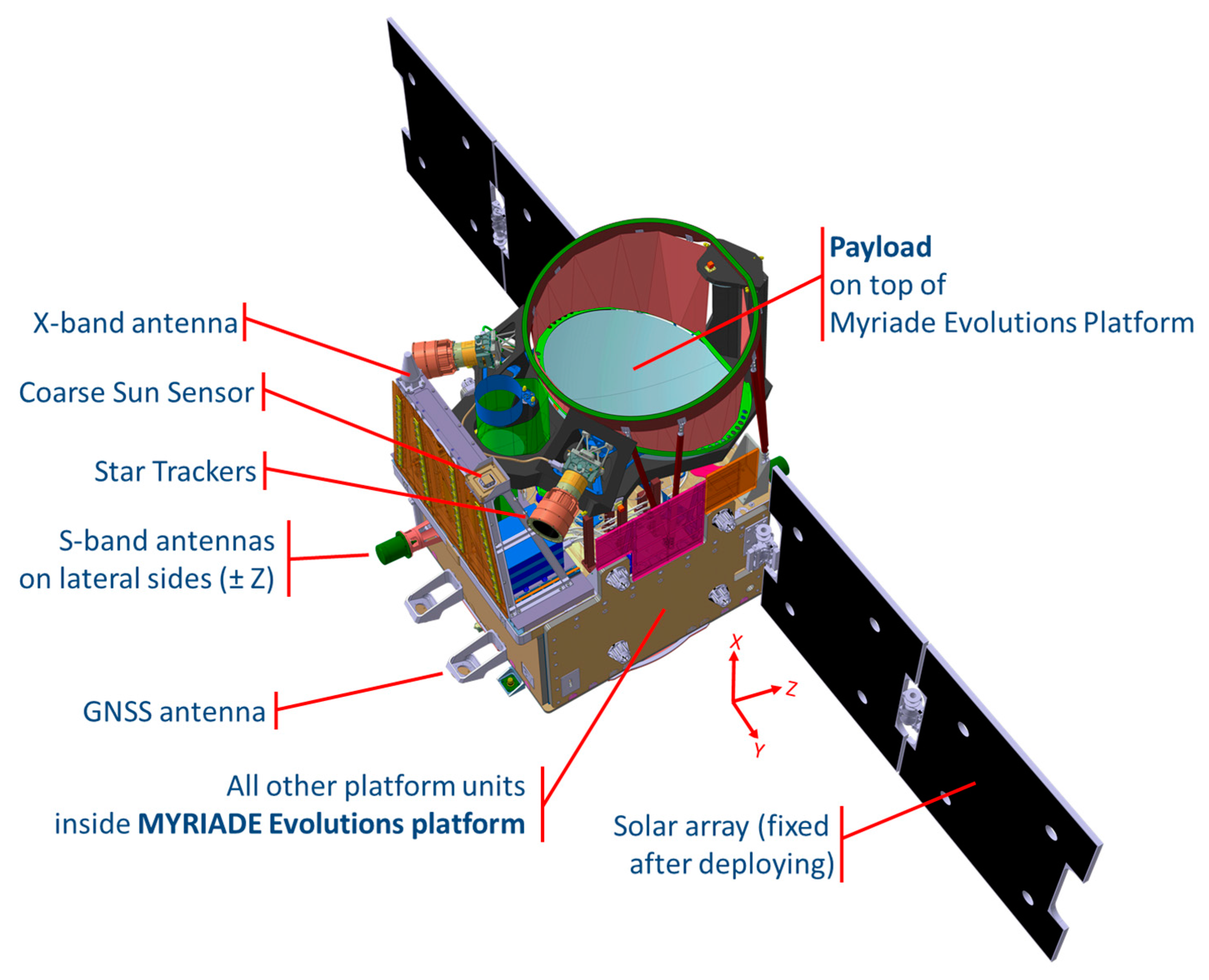
| Platform | MYRIADE Evolutions |
|---|---|
| Satellite Mass (Platform+Payload): | 430 kg |
| Satellite Power (Platform+Payload): | 500 W |
| GPS receiver: | 2 sensors |
| Star tracker: | 2 optical Heads |
| Payload: | IPDA Lidar for Methane |
| Mass allocation: | 140 kg |
| Power allocation: | 150 W |
| Laser transmitter type: | Nd:YAG pumped OPO |
| Online frequency: | 6076.9896 cm−1 |
| Offline frequency: | 6075.97 cm−1 |
| Pulse energy: | 9.5 mJ |
| Pulse length: | 20 ns |
| Time lag between on/offline transmission: | 250 µs |
| Pulse-pair repetition rate: | 20 Hz |
| Receiving telescope size: | 69 cm |
| Detector type: | Avalanche Pin Diode (APD) |
| Spot size on ground | 100 m (90% encircled energy) |
| Orbit: | Sun synchr. polar, low Earth orbit (LEO) |
| LTAN: | 06:00 h or 18:00 h |
| Height: | ~500 km |
| Inclination: | 97.4° |
| Repeat cycle: | 28 days |
| Attitude control: | 3 axis stabilized |
| Parameter | User Requirements | MERLIN System Specification Requirement | ||
|---|---|---|---|---|
| Threshold | Breakthrough | Target | ||
| XCH4 random error | 36 ppb | 18 ppb | 8 ppb | 22 ppb (27 ppb *) |
| XCH4 systematic error | 3 ppb | 2 ppb | 1 ppb | 3 ppb (3.7 ppb *) |
| Spatial coverage | Global | Global | Global | Global |
| Resolution | Horizontal: 50 km averaging; vertical: total column | |||
| Parameter | Random Error | Impact on XCH4 |
|---|---|---|
| Differential Atmospheric Optical Depth (DAOD) | 1.3% | 23.14 ppb |
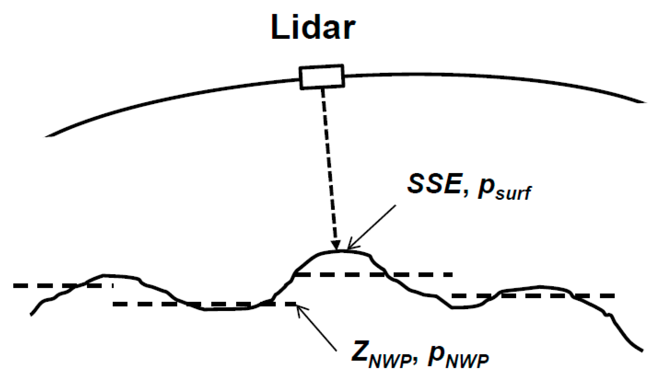
| SSE | 10 m | 2.57 ppb |
| Surface pressure (Numerical Weather Prediction (NWP)) | 2 hPa | 4.27 ppb |
| Temperature | 2 K | 5.2 ppb |
| Total budget based on specified values | 24.3 ppb |
| Parameter | Systematic Errors | Impact on XCH4 |
|---|---|---|
| DAOD | 0.13% | 2.31 ppb |
| SSE | 6 m | 1.54 ppb |
| Surface pressure (NWP) | 0.2 hPa | 0.43 ppb |
| Temperature | 2 profiles of bias | 0.5 ppb |
| Water vapor | 4% | 0.1 ppb |
| Methane cross section | 0.2% | 0.62 ppb |
| Frequency | 7 MHz offset, 8 MHz systematic | 0.3 ppb |
| Laser width knowledge | 5% for 100 MHz | 0.17 ppb |
| Spectral purity | - | 0.23 ppb |
| Processing | 1 ppb | |
| Total budget based on specified values | 3.1 ppb |
© 2017 by the authors. Licensee MDPI, Basel, Switzerland. This article is an open access article distributed under the terms and conditions of the Creative Commons Attribution (CC BY) license (http://creativecommons.org/licenses/by/4.0/).
Share and Cite
Ehret, G.; Bousquet, P.; Pierangelo, C.; Alpers, M.; Millet, B.; Abshire, J.B.; Bovensmann, H.; Burrows, J.P.; Chevallier, F.; Ciais, P.; et al. MERLIN: A French-German Space Lidar Mission Dedicated to Atmospheric Methane. Remote Sens. 2017, 9, 1052. https://doi.org/10.3390/rs9101052
Ehret G, Bousquet P, Pierangelo C, Alpers M, Millet B, Abshire JB, Bovensmann H, Burrows JP, Chevallier F, Ciais P, et al. MERLIN: A French-German Space Lidar Mission Dedicated to Atmospheric Methane. Remote Sensing. 2017; 9(10):1052. https://doi.org/10.3390/rs9101052
Chicago/Turabian StyleEhret, Gerhard, Philippe Bousquet, Clémence Pierangelo, Matthias Alpers, Bruno Millet, James B. Abshire, Heinrich Bovensmann, John P. Burrows, Frédéric Chevallier, Philippe Ciais, and et al. 2017. "MERLIN: A French-German Space Lidar Mission Dedicated to Atmospheric Methane" Remote Sensing 9, no. 10: 1052. https://doi.org/10.3390/rs9101052