Nominal 30-m Cropland Extent Map of Continental Africa by Integrating Pixel-Based and Object-Based Algorithms Using Sentinel-2 and Landsat-8 Data on Google Earth Engine


 , , and
Abstract
:
1. Introduction
2. Materials
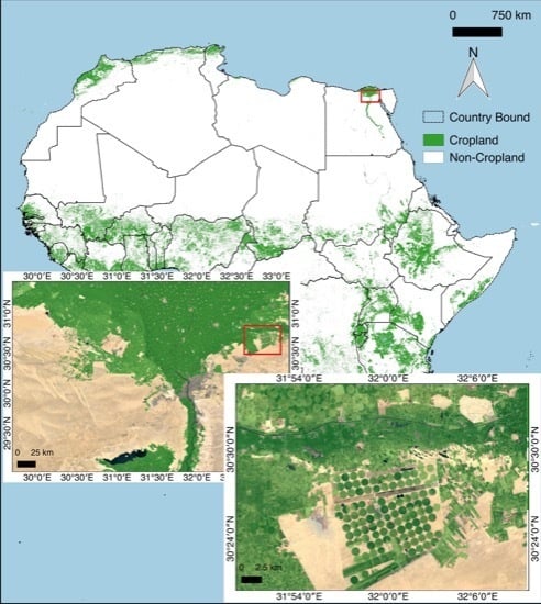
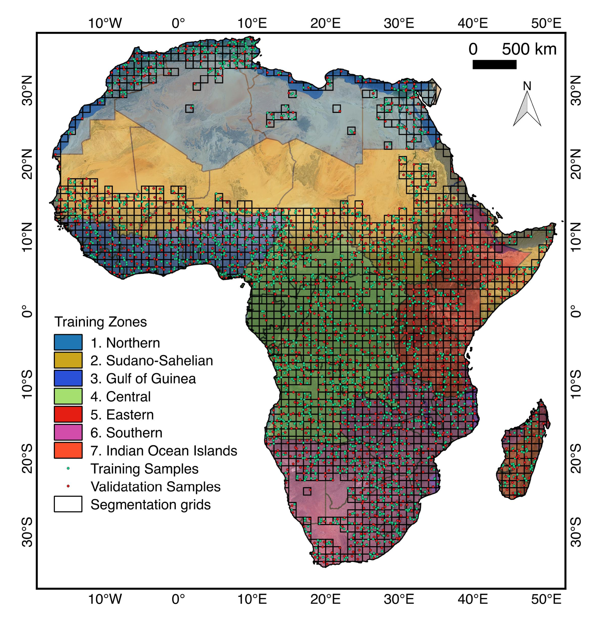
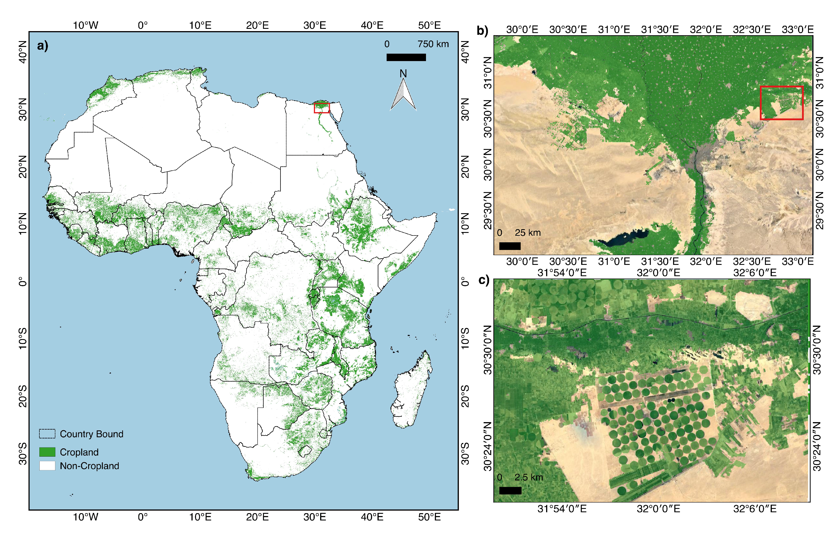
2.1. Study Area
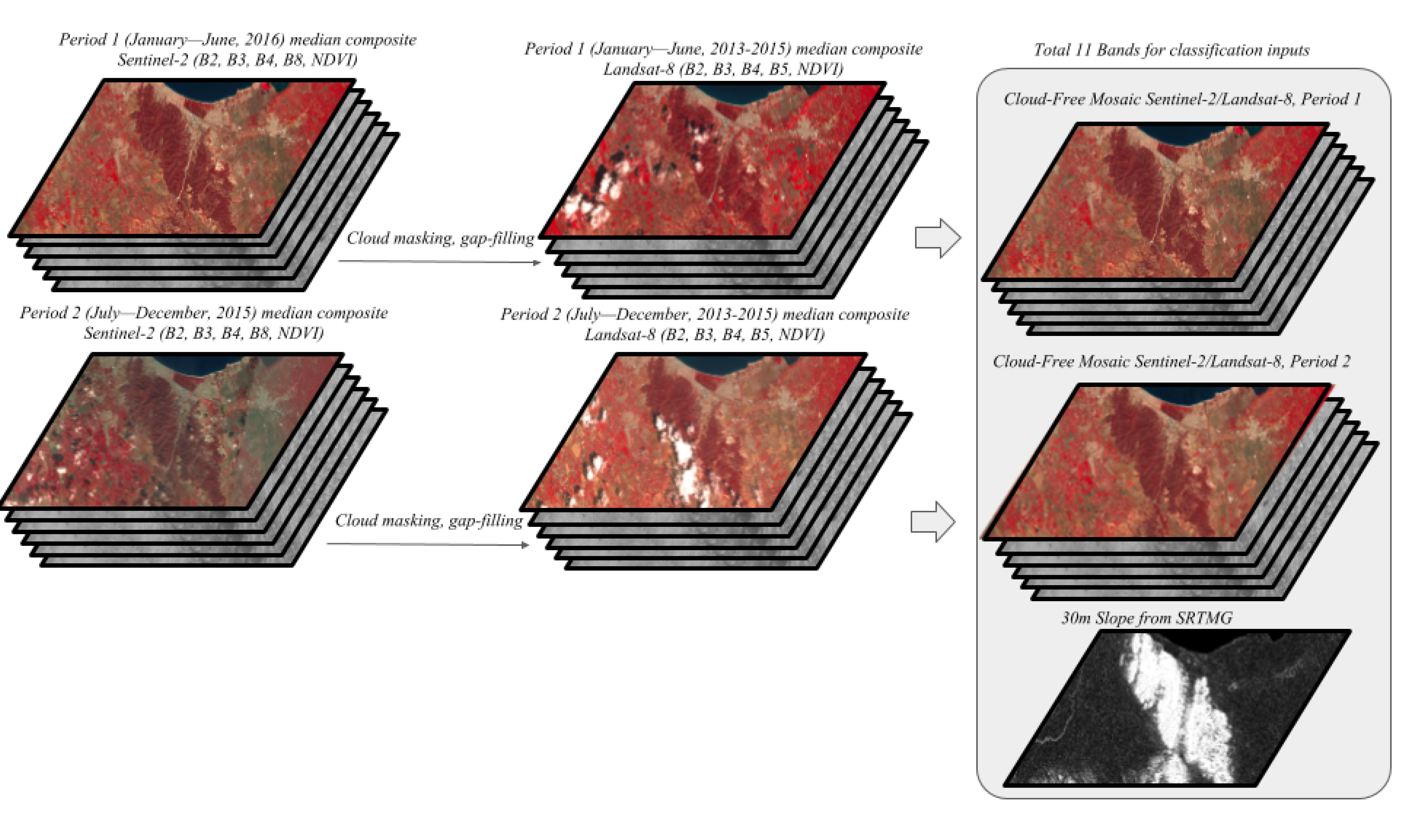
2.2. Cloud-Free Satellite Imagery Composition at 30-m Resolution
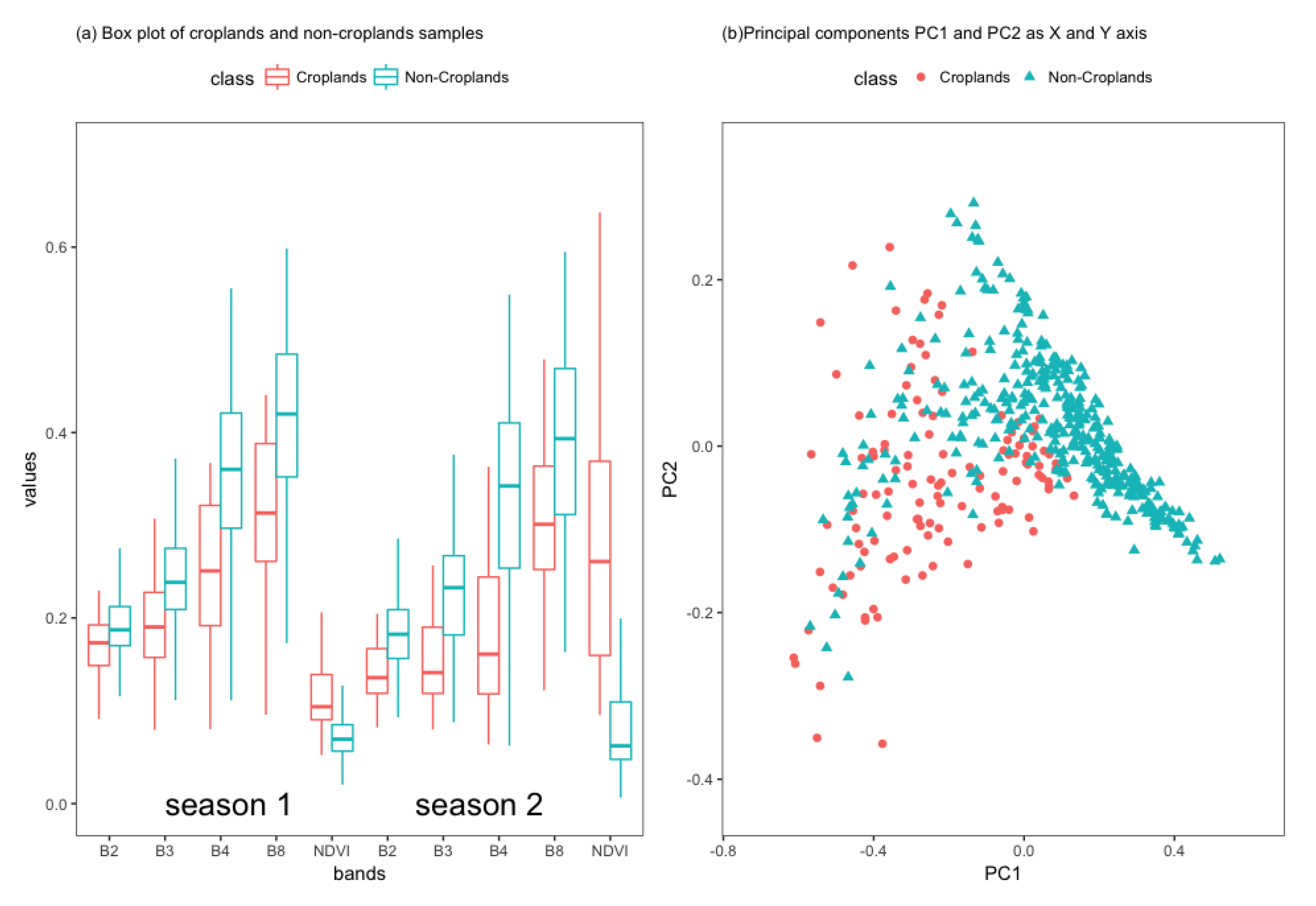
2.3. Reference Training Samples
2.4. Reference Validation Sample Polygons
3. Methods
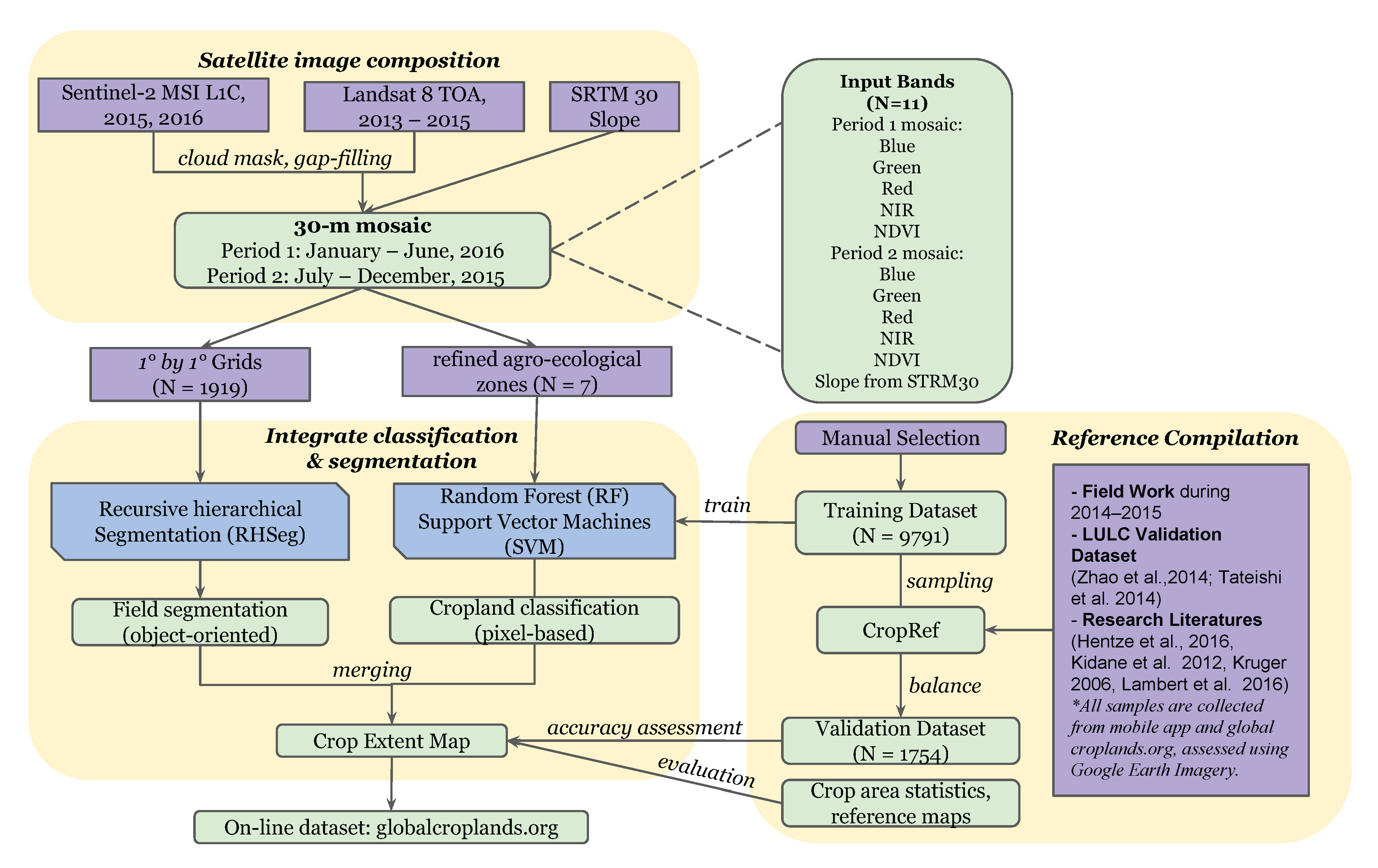
3.1. Overview of the Methodology
- 30-m mosaic (11 bands) was built using Sentinel-2 and Landsat-8 data (Section 2.2) for period 1 (January–June, 2016) and period 2 (July–December, 2015);
- Random Forest and Support Vector Machines (Section 3.1) were used to classify input bands for croplands versus non-croplands;
- Using same bands as inputs, recursive hierarchical segmentation (Section 3.2) was carried out in 1 by 1 grid units on NASA pleiades supercomputer;
- The pixel-based classification was integrated with object-based segmentation into cropland extent map (Section 3.3) for further assessment (Section 3.4)
- We compared derived cropland areas with country-wise statistics from other sources in Section 3.5 and explored the consistency between GFSAD30AFCE map and other reference maps in Section 3.6.
- 30-m Cropland extent product is released through the NASA Land Processes Distributed Active Archive Center (LP DAAC) at: https://doi.org/10.5067/MEaSUREs/GFSAD/GFSAD30AFCE.001 and can be viewed at: https://croplands.org.
3.2. Pixel-Based Classifier: Random Forest (RF) and Support Vector Machine (SVM)
3.3. Recursive Hierarchical Image Segmentation (RHSeg)
3.4. Integration of Pixel-Based Classification and Object-Based Segmentation
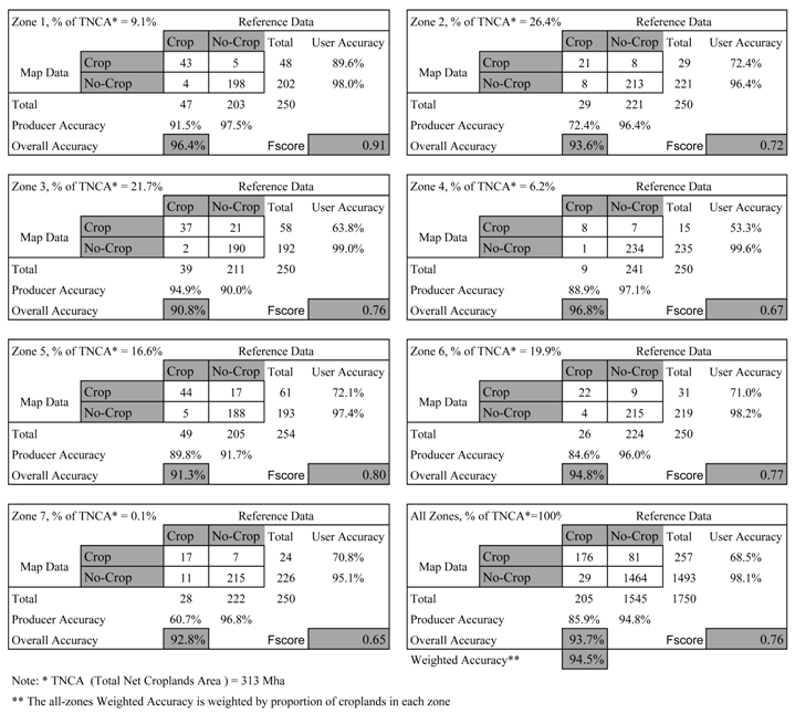
3.5. Accuracy Assessment
- Stratified, random and balanced sampling: The African continent has been divided into 7 refined agro-ecological zones or RAEZs (Figure 1) for stratified random sampling. Due to a large crop diversity across RAEZ’s (Figure 1) there is high variability in their growing periods and crop distribution. Therefore, to maintain balanced sampling for each zone, samples have been randomly distributed in each zone. The question of how many samples are sufficient to achieve statistically valid accuracy results is described in next point below.
- Sample Size: The sample size has been chosen based on the analysis of incrementing minimum number of samples. Initially, first 50 samples were chosen as minimum number for all the 7 RAE’s and then incremented in steps with another 50 more samples. A few RAEZ’s in Africa have little cropland distribution so that 50 samples were enough to achieve a valid assessment. However, other RAEZ’s needed up to 250 samples for their assessment. Beyond 250 samples, accuracies of all RAEZ’s become asymptotic. Overall, for Africa, total 1754 samples were used from 7 RAEZ’s.
- Sample unit: The sample unit for a given validation sample must be a group of pixels (at least 3 × 3 pixels of 30-m resolution) in order to minimize the impact of positional accuracy [88]. This sampling unit is a 3 × 3 homogeneous window containing one class. If a sample at this step was recognized to be a mixed patch of cropland and non-cropland, it had to be excluded from the validation dataset in the accuracy assessment since heterogeneous windows were not considered, however excluding them is the best practical choice for accuracy assessment.
- Sampling was balanced to keep the proportion of the cropland versus non-cropland samples close to the proportion of the cropland versus non-cropland area from the product layer to be validated.
- Validation samples are created independently from training samples described in Section 2.3, by a different team.
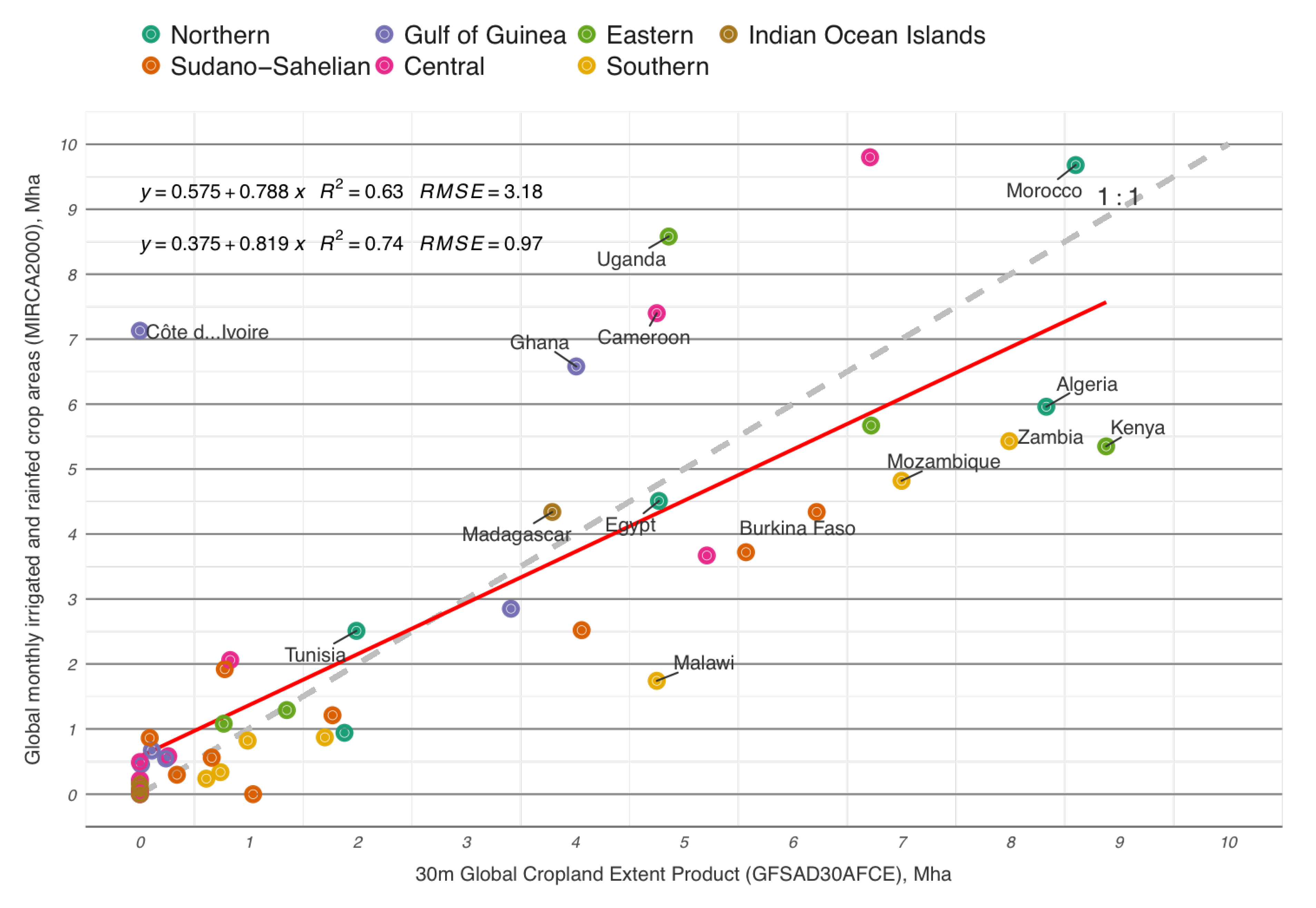
3.6. Calculation of Actual Cropland Areas and Comparison with Areas from Other Sources
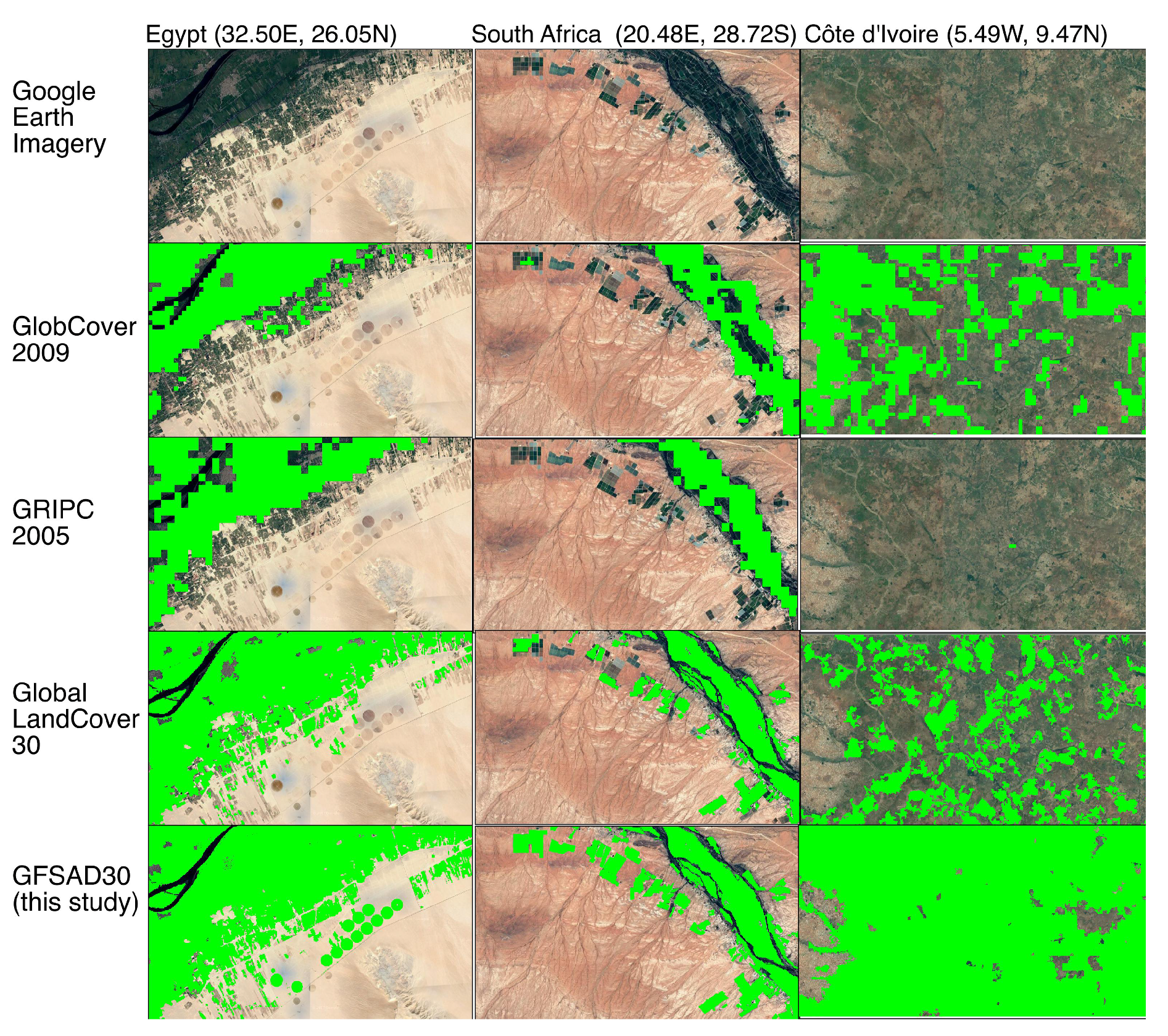
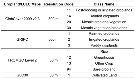
3.7. Consistency between GFSAD30AFCE Product and Four Existing Crop Maps
- Global Land Cover Map for 2009 (GlobCover 2009) [39]. Class 11, 14 were reclassified as “croplands” and other land cover classes were reclassified as “non-croplands”;
- Global rainfed, irrigated, and paddy croplands map GRIPC [16]. All agricultural classes include rainfed, irrigated and paddy were combined as “croplands” and other classes were “non-croplands”;
- 30-m global land-cover map FROM-GLC [48]. Level 1 class 10 and Level 2 Bare-cropland 94 were combined as “croplands” and other classes were “non-croplands”; and
- Global land cover GLC30 [45]. Class 10 was combined as “croplands” and other classes were “non-croplands”.
4. Results
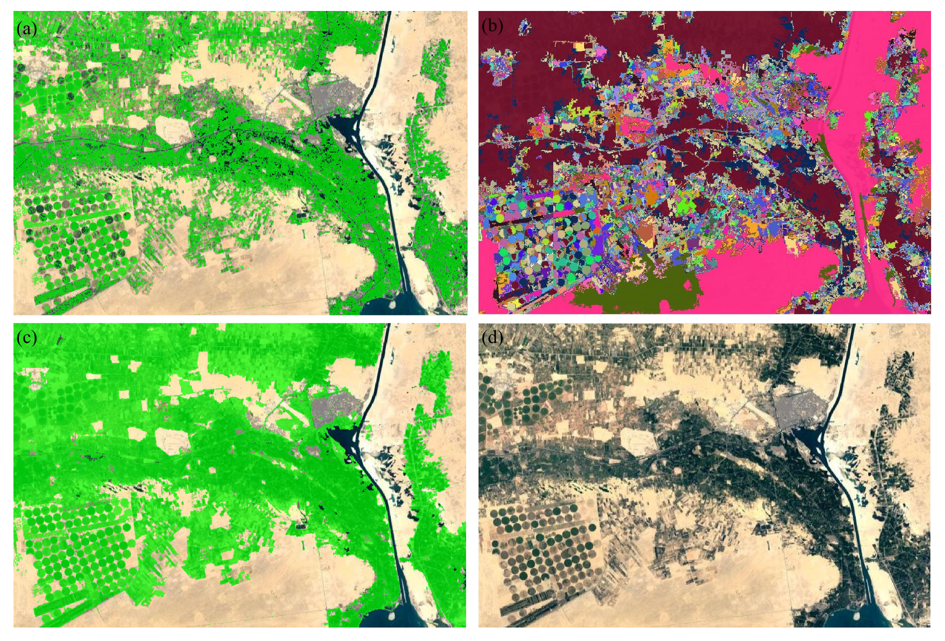
4.1. GFSAD30AFCE Product
4.2. GFSAD30AFCE Product Accuracies
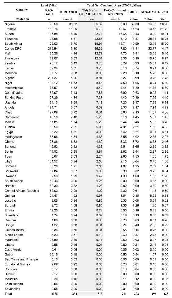
4.3. Cropland Areas and Comparison with Statistics from Other Sources
- Different definition of “croplands” class: GFSAD30AFCE product as per definition, includes all agricultural annual standing croplands, cropland fallows, and permanent plantation crops whereas cropland areas reported in statistics may not include cropland fallows;
- Different time: GFSAD30AFCE incorporate the latest cultivated area in 2015–2016 as well as the croplands fallows whereas country reported cropland areas may happen in other years.
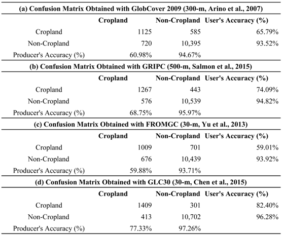
4.4. Consistency between GFSAD30AFCE Product and Four Existing Crop Maps
5. Discussion
6. Conclusions
Acknowledgments
Author Contributions
Conflicts of Interest
Abbreviations
| GFSAD30: | Global Food Security Analysis-Support Data Project |
| GEE: | Google Earth Engine |
References
- Thenkabail, P.S.; Hanjra, M.A.; Dheeravath, V.; Gumma, M. A Holistic View of Global Croplands and Their Water Use for Ensuring Global Food Security in the 21st Century through Advanced Remote Sensing and Non-remote Sensing Approaches. Remote Sens. 2010, 2, 211–261. [Google Scholar] [CrossRef] [Green Version]
- Fritz, S.; See, L.; Rembold, F. Comparison of global and regional land cover maps with statistical information for the agricultural domain in Africa. Int. J. Remote Sens. 2010, 31, 2237–2256. [Google Scholar] [CrossRef]
- Herold, M.; Mayaux, P.; Woodcock, C.E.; Baccini, A.; Schmullius, C. Some challenges in global land cover mapping: An assessment of agreement and accuracy in existing 1 km datasets. Remote Sens. Environ. 2008, 112, 2538–2556. [Google Scholar] [CrossRef]
- See, L.; Fritz, S.; You, L.; Ramankutty, N.; Herrero, M.; Justice, C.; Becker-Reshef, I.; Thornton, P.; Erb, K.; Gong, P.; et al. Improved global cropland data as an essential ingredient for food security. Glob. Food Secur. 2015, 4, 37–45. [Google Scholar] [CrossRef] [Green Version]
- Delrue, J.; Bydekerke, L.; Eerens, H.; Gilliams, S.; Piccard, I.; Swinnen, E. Crop mapping in countries with small-scale farming: A case study for West Shewa, Ethiopia. Int. J. Remote Sens. 2012, 34, 2566–2582. [Google Scholar] [CrossRef]
- Hannerz, F.; Lotsch, A. Assessment of land use and cropland inventories for Africa. In CEEPA Discussion Papers; University of Pretoria: Pretoria, South Africa, 2006; Volume 22. [Google Scholar]
- Gallego, F.J.; Kussul, N.; Skakun, S.; Kravchenko, O.; Shelestov, A.; Kussul, O. Efficiency assessment of using satellite data for crop area estimation in Ukraine. Int. J. Appl. Earth Obs. Geoinf. 2014, 29, 22–30. [Google Scholar] [CrossRef]
- Thenkabail, P.S.; Wu, Z. An Automated Cropland Classification Algorithm (ACCA) for Tajikistan by Combining Landsat, MODIS, and Secondary Data. Remote Sens. 2012, 4, 2890–2918. [Google Scholar] [CrossRef]
- Wu, W.; Shibasaki, R.; Yang, P.; Zhou, Q.; Tang, H. Remotely sensed estimation of cropland in China: A comparison of the maps derived from four global land cover datasets. Can. J. Remote Sens. 2014, 34, 467–479. [Google Scholar] [CrossRef]
- Büttner, G. CORINE Land Cover and Land Cover Change Products. In Land Use and Land Cover Mapping in Europe; Springer: Dordrecht, The Netherlands, 2014; pp. 55–74. [Google Scholar]
- Tian, S.; Zhang, X.; Tian, J.; Sun, Q. Random Forest Classification of Wetland Landcovers from Multi-Sensor Data in the Arid Region of Xinjiang, China. Remote Sens. 2016, 8, 954. [Google Scholar] [CrossRef]
- Pittman, K.; Hansen, M.C.; Becker-Reshef, I.; Potapov, P.V.; Justice, C.O. Estimating Global Cropland Extent with Multi-year MODIS Data. Remote Sens. 2010, 2, 1844–1863. [Google Scholar] [CrossRef]
- Thenkabail, P.S.; Biradar, C.M.; Noojipady, P.; Dheeravath, V.; Li, Y.; Velpuri, M.; Gumma, M.; Gangalakunta, O.R.P.; Turral, H.; Cai, X.; et al. Global irrigated area map (GIAM), derived from remote sensing, for the end of the last millennium. Int. J. Remote Sens. 2009, 30, 3679–3733. [Google Scholar] [CrossRef]
- Teluguntla, P.; Thenkabail, P.S.; Xiong, J.; Gumma, M.K.; Congalton, R.G.; Oliphant, A.; Poehnelt, J.; Yadav, K.; Rao, M.N.; Massey, R. Spectral Matching Techniques (SMTs) and Automated Cropland Classification Algorithms (ACCAs) for Mapping Croplands of Australia using MODIS 250-m Time-series (2000–2015) Data. Int. J. Digit. Earth 2017, 944–977. [Google Scholar] [CrossRef]
- Xiong, J.; Thenkabail, P.S.; Gumma, M.K.; Teluguntla, P.; Poehnelt, J.; Congalton, R.G.; Yadav, K.; Thau, D. Automated cropland mapping of continental Africa using Google Earth Engine cloud computing. ISPRS J. Photogramm. Remote Sens. 2017, 126, 225–244. [Google Scholar] [CrossRef]
- Salmon, J.M.; Friedl, M.A.; Frolking, S.; Wisser, D.; Douglas, E.M. Global rain-fed, irrigated, and paddy croplands: A new high resolution map derived from remote sensing, crop inventories and climate data. Int. J. Appl. Earth Obs. Geoinf. 2015, 38, 321–334. [Google Scholar] [CrossRef]
- Alcántara, C.; Kuemmerle, T.; Prishchepov, A.V.; Radeloff, V.C. Mapping abandoned agriculture with multi-temporal MODIS satellite data. Remote Sens. Environ. 2012, 124, 334–347. [Google Scholar] [CrossRef]
- Estel, S.; Kuemmerle, T.; Alcántara, C.; Levers, C.; Prishchepov, A.; Hostert, P. Mapping farmland abandonment and recultivation across Europe using MODIS NDVI time series. Remote Sens. Environ. 2015, 163, 312–325. [Google Scholar] [CrossRef]
- Friedl, M.A.; Sulla-Menashe, D.; Tan, B.; Schneider, A.; Ramankutty, N.; Sibley, A.; Huang, X. MODIS Collection 5 global land cover: Algorithm refinements and characterization of new datasets. Remote Sens. Environ. 2010, 114, 168–182. [Google Scholar] [CrossRef]
- Boryan, C.; Yang, Z.; Mueller, R.; Craig, M. Monitoring US agriculture: The US Department of Agriculture, National Agricultural Statistics Service, Cropland Data Layer Program. Geocarto Int. 2011, 26, 341–358. [Google Scholar] [CrossRef]
- Vintrou, E.; Desbrosse, A.; Bégué, A.; Traoré, S. Crop area mapping in West Africa using landscape stratification of MODIS time series and comparison with existing global land products. Int. J. Appl. Earth Obs. Geoinf. 2012, 14, 83–93. [Google Scholar] [CrossRef]
- Dheeravath, V.; Thenkabail, P.S.; Thenkabail, P.S.; Noojipady, P.; Chandrakantha, G.; Reddy, G.P.O.; Gumma, M.K.; Biradar, C.M.; Velpuri, M.; Gumma, M.K. Irrigated areas of India derived using MODIS 500 m time series for the years 2001–2003. ISPRS J. Photogramm. Remote Sens. 2010, 65. [Google Scholar] [CrossRef]
- Biradar, C.M.; Thenkabail, P.S.; Noojipady, P.; Li, Y.; Dheeravath, V.; Turral, H.; Velpuri, M.; Gumma, M.K.; Gangalakunta, O.R.P.; Cai, X.L.; et al. A global map of rainfed cropland areas (GMRCA) at the end of last millennium using remote sensing. Int. J. Appl. Earth Obs. Geoinf. 2009, 11, 114–129. [Google Scholar] [CrossRef]
- Lambert, M.J.; Waldner, F.; Defourny, P. Cropland Mapping over Sahelian and Sudanian Agrosystems: A Knowledge-Based Approach Using PROBA-V Time Series at 100-m. Remote Sens. 2016, 8. [Google Scholar] [CrossRef]
- Shao, Y.; Lunetta, R.S. Comparison of support vector machine, neural network, and CART algorithms for the land-cover classification using limited training data points. ISPRS J. Photogramm. Remote Sens. 2012, 70, 78–87. [Google Scholar] [CrossRef]
- Kussul, N.; Skakun, S.; Shelestov, A. Regional scale crop mapping using multi-temporal satellite imagery. Int. Arch. Photogramm. Remote Sens. Spat. Inf. Sci. 2015, 40, 45–52. [Google Scholar] [CrossRef]
- Skakun, S.; Kussul, N.; Shelestov, A.Y.; Lavreniuk, M.; Kussul, O. Efficiency Assessment of Multitemporal C-Band Radarsat-2 Intensity and Landsat-8 Surface Reflectance Satellite Imagery for Crop Classification in Ukraine. IEEE J. Sel. Top. Appl. Earth Obs. Remote Sens. 2015, 9, 3712–3719. [Google Scholar] [CrossRef]
- Huang, C.; Davis, L.S.; Townshend, J.R.G. An assessment of support vector machines for land cover classification. Int. J. Remote Sens. 2010, 23, 725–749. [Google Scholar] [CrossRef]
- Vintrou, E.; Ienco, D.; Bégué, A. Data mining, a promising tool for large-area cropland mapping. IEEE J. Sel. Top. Appl. Earth Obs. Remote Sens. 2013, 6, 2132–2138. [Google Scholar] [CrossRef]
- Pan, Y.; Hu, T.; Zhu, X.; Zhang, J. Mapping cropland distributions using a hard and soft classification model. IEEE Trans. Geosci. Remote Sens. 2012, 50, 4301–4312. [Google Scholar] [CrossRef]
- Van Niel, T.G.; McVicar, T.R. Determining temporal windows for crop discrimination with remote sensing: A case study in south-eastern Australia. Comput. Electron. Agric. 2004, 45, 91–108. [Google Scholar] [CrossRef]
- Conrad, C.; Dech, S.; Dubovyk, O.; Fritsch, S.; Klein, D.; Löw, F.; Schorcht, G.; Zeidler, J. Derivation of temporal windows for accurate crop discrimination in heterogeneous croplands of Uzbekistan using multitemporal RapidEye images. Comput. Electron. Agric. 2014, 103, 63–74. [Google Scholar] [CrossRef]
- Löw, F.; Michel, U.; Dech, S.; Conrad, C. Impact of feature selection on the accuracy and spatial uncertainty of per-field crop classification using Support Vector Machines. ISPRS J. Photogramm. Remote Sens. 2013, 85, 102–119. [Google Scholar] [CrossRef]
- Matton, N.; Canto, G.; Waldner, F.; Valero, S.; Morin, D.; Inglada, J.; Arias, M.; Bontemps, S.; Koetz, B.; Defourny, P. An Automated Method for Annual Cropland Mapping along the Season for Various Globally-Distributed Agrosystems Using High Spatial and Temporal Resolution Time Series. Remote Sens. 2015, 7, 13208–13232. [Google Scholar] [CrossRef]
- Peña-Barragán, J.M.; Ngugi, M.K.; Plant, R.E.; Six, J. Object-based crop identification using multiple vegetation indices, textural features and crop phenology. Remote Sens. Environ. 2011, 115, 1301–1316. [Google Scholar] [CrossRef]
- Johnson, D.M.; Mueller, R. The 2009 Cropland Data Layer. Photogramm. Eng. Remote Sens. 2010, 76, 1201–1205. [Google Scholar]
- Kalensky, Z.D. AFRICOVER Land Cover Database and Map of Africa. Can. J. Remote Sens. 1998, 24, 292–297. [Google Scholar] [CrossRef]
- Bartholomé, E.; Belward, A.S. GLC2000: A new approach to global land cover mapping from Earth observation data. Int. J. Remote Sens. 2005, 26, 1959–1977. [Google Scholar] [CrossRef]
- Arino, O.; Gross, D.; Ranera, F.; Leroy, M.; Bicheron, P.; Brockman, C.; Defourny, P.; Vancutsem, C.; Achard, F.; Durieux, L.; et al. GlobCover: ESA service for global land cover from MERIS. In Proceedings of the IEEE International Geoscience and Remote Sensing Symposium, Barcelona, Spain, 23–27 July 2007; pp. 2412–2415. [Google Scholar]
- Latham, J.; Cumani, R.; Rosati, I.; Bloise, M. Global Land Cover Share (GLC-SHARE) Database Beta-Release Version 1.0-2014; FAO: Rome, Italy, 2014; Available online: http://csdms.colorado.edu/wiki/Data:GLC-SHARE (accessed on 31 May 2017).
- Friedl, M.A.; McIver, D.K.; Hodges, J.C.F.; Zhang, X.Y.; Muchoney, D.; Strahler, A.H.; Woodcock, C.E.; Gopal, S.; Schneider, A.; Cooper, A.; et al. Global land cover mapping from MODIS: algorithms and early results. Remote Sens. Environ. 2002, 83, 287–302. [Google Scholar] [CrossRef]
- Waldner, F.; Fritz, S.; Di Gregorio, A.; Defourny, P. Mapping Priorities to Focus Cropland Mapping Activities: Fitness Assessment of Existing Global, Regional and National Cropland Maps. Remote Sens. 2015, 7, 7959–7986. [Google Scholar] [CrossRef] [Green Version]
- Teluguntla, P.; Thenkabail, P.; Xiong, J.; Gumma, M.K.; Giri, C.; Milesi, C.; Ozdogan, M.; Congalton, R.; Yadav, K. CHAPTER 6—Global Food Security Support Analysis Data at Nominal 1 km (GFSAD1 km) Derived from Remote Sensing in Support of Food Security in the Twenty-First Century: Current Achievements and Future Possibilities. In Remote Sensing Handbook (Volume II): Land Resources Monitoring, Modeling, and Mapping with Remote Sensing; Thenkabail, P.S., Ed.; CRC Press: Boca Raton, FL, USA; London, UK; New York, NY, USA, 2015; pp. 131–160. [Google Scholar]
- Waldner, F.; De Abelleyra, D.; Verón, S.R.; Zhang, M.; Wu, B.; Plotnikov, D.; Bartalev, S.; Lavreniuk, M.; Skakun, S.; Kussul, N.; et al. Towards a set of agrosystem-specific cropland mapping methods to address the global cropland diversity. Int. J. Remote Sens. 2016, 37, 3196–3231. [Google Scholar] [CrossRef] [Green Version]
- Chen, J.; Chen, J.; Liao, A.; Cao, X.; Chen, L.; Chen, X.; He, C.; Han, G.; Peng, S.; Zhang, W.; et al. Global land cover mapping at 30 m resolution: A POK-based operational approach. ISPRS J. Photogramm. Remote Sens. 2015, 103, 7–27. [Google Scholar] [CrossRef]
- Gong, P.; Wang, J.; Yu, L.; Zhao, Y.; Zhao, Y.; Liang, L.; Niu, Z.; Huang, X.; Fu, H.; Liu, S.; et al. Finer resolution observation and monitoring of global land cover: first mapping results with Landsat TM and ETM+ data. Int. J. Remote Sens. 2013, 34, 2607–2654. [Google Scholar] [CrossRef]
- Hansen, M.C.; Loveland, T.R. A review of large area monitoring of land cover change using Landsat data. Remote Sens. Environ. 2012, 122, 66–74. [Google Scholar] [CrossRef]
- Yu, L.; Wang, J.; Clinton, N.; Xin, Q.; Chen, Y.; Zhong, L.; Gong, P. FROM-GC: 30 m global cropland extent derived through multisource data integration. Int. J. Digit. Earth 2013, 6, 521–533. [Google Scholar] [CrossRef]
- Costa, H.; Carrão, H.; Bação, F.; Caetano, M. Combining per-pixel and object-based classifications for mapping land cover over large areas. Int. J. Remote Sens. 2014, 35, 738–753. [Google Scholar] [CrossRef]
- Myint, S.W.; Gober, P.; Brazel, A.; Gober, P.; Brazel, A.; Grossman-Clarke, S.; Grossman-Clarke, S.; Weng, Q. Per-pixel vs. object-based classification of urban land cover extraction using high spatial resolution imagery. Remote Sens. Environ. 2011, 115, 1145–1161. [Google Scholar] [CrossRef]
- Malinverni, E.S.; Tassetti, A.N.; Mancini, A.; Zingaretti, P.; Frontoni, E.; Bernardini, A. Hybrid object-based approach for land use/land cover mapping using high spatial resolution imagery. Int. J. Geogr. Inf. Sci. 2011, 25, 1025–1043. [Google Scholar] [CrossRef]
- Dingle Robertson, L.; King, D.J. Comparison of pixel- and object-based classification in land cover change mapping. Int. J. Remote Sens. 2011, 32, 1505–1529. [Google Scholar] [CrossRef]
- Ok, A.O.; Akar, O.; Gungor, O. Evaluation of random forest method for agricultural crop classification. Eur. J. Remote Sens. 2012, 45, 421–432. [Google Scholar] [CrossRef]
- De Wit, A.J.W.; Clevers, J.G.P.W. Efficiency and accuracy of per-field classification for operational crop mapping. Int. J. Remote Sens. 2010, 25, 4091–4112. [Google Scholar] [CrossRef]
- Castillejo-González, I.L.; López-Granados, F.; García-Ferrer, A.; Peña-Barragán, J.M.; Jurado-Expósito, M.; de la Orden, M.S.; González-Audicana, M. Object- and pixel-based analysis for mapping crops and their agro-environmental associated measures using QuickBird imagery. Comput. Electron. Agric. 2009, 68, 207–215. [Google Scholar] [CrossRef]
- Marshall, M.T.; Husak, G.J.; Michaelsen, J.; Funk, C.; Pedreros, D.; Adoum, A. Testing a high-resolution satellite interpretation technique for crop area monitoring in developing countries. Int. J. Remote Sens. 2011, 32, 7997–8012. [Google Scholar] [CrossRef]
- Gorelick, N.; Hancher, M.; Dixon, M.; Ilyushchenko, S.; Thau, D.; Moore, R. Google Earth Engine: Planetary-scale geospatial analysis for everyone. Remote Sens. Environ. 2017. [Google Scholar] [CrossRef]
- Lupien, J.R. Agriculture Food and Nutrition for Africa–A Resource Book for Teachers of Agriculture; FAO: Rome, Italy, 1997; Available online: http://www.fao.org/docrep/w0078e/w0078e00.htm (accessed on 12 October 2016).
- Gerland, P.; Raftery, A.E.; ikova, H.E.; Li, N.; Gu, D.; Spoorenberg, T.; Alkema, L.; Fosdick, B.K.; Chunn, J.; Lalic, N.; et al. World population stabilization unlikely this century. Science 2014, 346, 234–237. [Google Scholar] [CrossRef] [PubMed]
- Drusch, M.; Del Bello, U.; Carlier, S.; Colin, O.; Fernandez, V.; Gascon, F.; Hoersch, B.; Isola, C.; Laberinti, P.; Martimort, P.; et al. Sentinel-2: ESA’s Optical High-Resolution Mission for GMES Operational Services. Remote Sens. Environ. 2012, 120, 25–36. [Google Scholar] [CrossRef]
- Immitzer, M.; Vuolo, F.; Atzberger, C. First Experience with Sentinel-2 Data for Crop and Tree Species Classifications in Central Europe. Remote Sens. 2016, 8, 166. [Google Scholar] [CrossRef]
- Battude, M.; Al Bitar, A.; Morin, D.; Cros, J.; Huc, M.; Sicre, C.M.; Le Dantec, V.; Demarez, V. Estimating maize biomass and yield over large areas using high spatial and temporal resolution Sentinel-2 like remote sensing data. Remote Sens. Environ. 2016, 184, 668–681. [Google Scholar] [CrossRef]
- Inglada, J.; Arias, M.; Tardy, B.; Hagolle, O.; Valero, S.; Morin, D.; Dedieu, G.; Sepulcre, G.; Bontemps, S.; Defourny, P.; et al. Assessment of an Operational System for Crop Type Map Production Using High Temporal and Spatial Resolution Satellite Optical Imagery. Remote Sens. 2015, 7, 12356–12379. [Google Scholar] [CrossRef]
- Valero, S.; Morin, D.; Inglada, J.; Sepulcre, G.; Arias, M.; Hagolle, O.; Dedieu, G.; Bontemps, S.; Defourny, P.; Koetz, B. Production of a Dynamic Cropland Mask by Processing Remote Sensing Image Series at High Temporal and Spatial Resolutions. Remote Sens. 2016, 8, 55. [Google Scholar] [CrossRef]
- Lohou, F.; Kergoat, L.; Guichard, F.; Boone, A.; Cappelaere, B.; Cohard, J.M.; Demarty, J.; Galle, S.; Grippa, M.; Peugeot, C.; et al. Surface response to rain events throughout the West African monsoon. Atmos. Chem. Phys. 2014, 14, 3883–3898. [Google Scholar] [CrossRef] [Green Version]
- Hentze, K.; Thonfeld, F.; Menz, G. Evaluating Crop Area Mapping from MODIS Time-Series as an Assessment Tool for Zimbabwe’s “Fast Track Land Reform Programme”. PLoS ONE 2016, 11. [Google Scholar] [CrossRef] [PubMed]
- Kidane, Y.; Stahlmann, R.; Beierkuhnlein, C. Vegetation dynamics, and land use and land cover change in the Bale Mountains, Ethiopia. Environ. Monit. Assess. 2012, 184, 7473–7489. [Google Scholar] [CrossRef] [PubMed]
- Kruger, A.C. Observed trends in daily precipitation indices in South Africa: 1910–2004. Int. J. Climatol. 2006, 26, 2275–2285. [Google Scholar] [CrossRef]
- Motha, R.P.; Leduc, S.K.; Steyaert, L.T.; Sakamoto, C.M.; Strommen, N.D.; Motha, R.P.; Leduc, S.K.; Steyaert, L.T.; Sakamoto, C.M.; Strommen, N.D. Precipitation Patterns in West Africa. Mon. Weather Rev. 1980, 108, 1567–1578. [Google Scholar] [CrossRef]
- D’Odorico, P.; Gonsamo, A.; Damm, A.; Schaepman, M.E. Experimental Evaluation of Sentinel-2 Spectral Response Functions for NDVI Time-Series Continuity. IEEE Trans. Geosci. Remote Sens. 2013, 51, 1336–1348. [Google Scholar] [CrossRef]
- Van der Werff, H.; van der Meer, F. Sentinel-2A MSI and Landsat 8 OLI Provide Data Continuity for Geological Remote Sensing. Remote Sens. 2016, 8, 883. [Google Scholar] [CrossRef]
- Storey, J.; Roy, D.P.; Masek, J.; Gascon, F.; Dwyer, J.; Choate, M. A note on the temporary misregistration of Landsat-8 Operational Land Imager (OLI) and Sentinel-2 Multi Spectral Instrument (MSI) imagery. Remote Sens. Environ. 2016, 186, 121–122. [Google Scholar] [CrossRef]
- Languille, F.; Déchoz, C.; Gaudel, A.; Greslou, D.; de Lussy, F.; Trémas, T.; Poulain, V. Sentinel-2 geometric image quality commissioning: First results. Proc. SPIE 2015, 9643, 964306. [Google Scholar] [CrossRef]
- Barazzetti, L.; Cuca, B.; Previtali, M. Evaluation of registration accuracy between Sentinel-2 and Landsat 8. Proc. SPIE 2016. [Google Scholar] [CrossRef]
- Farr, T.G.; Rosen, P.A.; Caro, E.; Crippen, R.; Duren, R.; Hensley, S.; Kobrick, M.; Paller, M.; Rodriguez, E.; Roth, L.; et al. The Shuttle Radar Topography Mission. Rev. Geophys. 2007, 45. [Google Scholar] [CrossRef]
- Aitkenhead, M.J.; Aalders, I.H. Automating land cover mapping of Scotland using expert system and knowledge integration methods. Remote Sens. Environ. 2011, 115, 1285–1295. [Google Scholar] [CrossRef]
- Pelletier, C.; Valero, S.; Inglada, J.; Champion, N.; Dedieu, G. Assessing the robustness of Random Forests to map land cover with high resolution satellite image time series over large areas. Remote Sens. Environ. 2016, 187, 156–168. [Google Scholar] [CrossRef]
- Sharma, R.; Tateishi, R.; Hara, K.; Iizuka, K. Production of the Japan 30-m Land Cover Map of 2013–2015 Using a Random Forests-Based Feature Optimization Approach. Remote Sens. 2016, 8, 429. [Google Scholar] [CrossRef]
- Wessels, K.; van den Bergh, F.; Roy, D.; Salmon, B.; Steenkamp, K.; MacAlister, B.; Swanepoel, D.; Jewitt, D. Rapid Land Cover Map Updates Using Change Detection and Robust Random Forest Classifiers. Remote Sens. 2016, 8, 888. [Google Scholar] [CrossRef]
- Vapnik, V.N.; Vapnik, V. Statistical Learning Theory; Wiley: New York, NY, USA, 1998. [Google Scholar]
- Shi, D.; Yang, X. Support Vector Machines for Land Cover Mapping from Remote Sensor Imagery. In Monitoring and Modeling of Global Changes: A Geomatics Perspective; Springer: Dordrecht, The Netherlands, 2015; pp. 265–279. [Google Scholar]
- Im, J.; Jensen, J.R.; Tullis, J.A. Object-based change detection using correlation image analysis and image segmentation. Int. J. Remote Sens. 2008, 29, 399–423. [Google Scholar] [CrossRef]
- Stow, D.; Hamada, Y.; Coulter, L.; Anguelova, Z. Monitoring shrubland habitat changes through object-based change identification with airborne multispectral imagery. Remote Sens. Environ. 2008, 112, 1051–1061. [Google Scholar] [CrossRef]
- Espindola, G.; Câmara, G.; Reis, I.; Bins, L.; Monteiro, A. Parameter selection for region-growing image segmentation algorithms using spatial autocorrelation. Int. J. Remote Sens. 2006, 27, 3035–3040. [Google Scholar] [CrossRef]
- Nemani, R.; Votava, P.; Michaelis, A.; Melton, F.; Milesi, C. Collaborative supercomputing for global change science. Eos Trans. Am. Geophys. Union 2011, 92, 109–110. [Google Scholar] [CrossRef]
- Tilton, J.C.; Tarabalka, Y.; Montesano, P.M.; Gofman, E. Best Merge Region-Growing Segmentation with Integrated Nonadjacent Region Object Aggregation. IEEE Trans. Geosci. Remote Sens. 2012, 50, 4454–4467. [Google Scholar] [CrossRef]
- Sulla-Menashe, D.; Friedl, M.A.; Krankina, O.N.; Baccini, A.; Woodcock, C.E.; Sibley, A.; Sun, G.; Kharuk, V.; Elsakov, V. Hierarchical mapping of Northern Eurasian land cover using MODIS data. Remote Sens. Environ. 2011, 115, 392–403. [Google Scholar] [CrossRef]
- Congalton, R.G.; Green, K. Assessing the Accuracy of Remotely Sensed Data: Principles and Practice, 2nd ed.; CRC/Taylor & Francis: Boca Raton, FL, USA, 2009; p. 183. [Google Scholar]
- Congalton, R.G. Assessing Positional and Thematic Accuracies of Maps Generated from Remotely Sensed Data. In “Remote Sensing Handbook” (Volume I): Remotely Sensed Data Characterization, Classification, and Accuracies; Thenkabail, P.S., Ed.; CRC Press: Boca Raton, FL, USA; London, UK; New York, NY, USA, 2015; pp. 583–602. [Google Scholar]
- Thenkabail, P.S.; Knox, J.W.; Ozdogan, M.; Gumma, M.K.; Congalton, R.G.; Wu, Z.; Milesi, C.; Finkral, A.; Marshall, M.; Mariotto, I.; et al. Assessing Future Risks to Agricultural Productivity, Water Resources and Food Security: How Can Remote Sensing Help? Photogramm. Eng. Remote Sens. 2012, 78, 773–782. [Google Scholar]
- Chapagain, A.K.; Hoekstra, A.Y. The global component of freshwater demand and supply: An assessment of virtual water flows between nations as a result of trade in agricultural and industrial products. Water Int. 2008, 33, 19–32. [Google Scholar] [CrossRef]
- Portmann, F.T.; Siebert, S.; Döll, P. MIRCA2000—Global monthly irrigated and rainfed crop areas around the year 2000: A new high-resolution data set for agricultural and hydrological modeling. Glob. Biogeochem. Cycles 2010, 24, 1–24. [Google Scholar] [CrossRef]
- Dorward, A.; Chirwa, E. A Review of Methods for Estimating Yield and Production Impacts. 2010. Available online: http://eprints.soas.ac.uk/16731/1/FISP%20Production%20Methodologies%20review%20Dec%20Final.pdf (accessed on 10 August 2016).


© 2017 by the authors. Licensee MDPI, Basel, Switzerland. This article is an open access article distributed under the terms and conditions of the Creative Commons Attribution (CC BY) license (http://creativecommons.org/licenses/by/4.0/).
Share and Cite
Xiong, J.; Thenkabail, P.S.; Tilton, J.C.; Gumma, M.K.; Teluguntla, P.; Oliphant, A.; Congalton, R.G.; Yadav, K.; Gorelick, N. Nominal 30-m Cropland Extent Map of Continental Africa by Integrating Pixel-Based and Object-Based Algorithms Using Sentinel-2 and Landsat-8 Data on Google Earth Engine. Remote Sens. 2017, 9, 1065. https://doi.org/10.3390/rs9101065
Xiong J, Thenkabail PS, Tilton JC, Gumma MK, Teluguntla P, Oliphant A, Congalton RG, Yadav K, Gorelick N. Nominal 30-m Cropland Extent Map of Continental Africa by Integrating Pixel-Based and Object-Based Algorithms Using Sentinel-2 and Landsat-8 Data on Google Earth Engine. Remote Sensing. 2017; 9(10):1065. https://doi.org/10.3390/rs9101065
Chicago/Turabian StyleXiong, Jun, Prasad S. Thenkabail, James C. Tilton, Murali K. Gumma, Pardhasaradhi Teluguntla, Adam Oliphant, Russell G. Congalton, Kamini Yadav, and Noel Gorelick. 2017. "Nominal 30-m Cropland Extent Map of Continental Africa by Integrating Pixel-Based and Object-Based Algorithms Using Sentinel-2 and Landsat-8 Data on Google Earth Engine" Remote Sensing 9, no. 10: 1065. https://doi.org/10.3390/rs9101065