The Methane Isotopologues by Solar Occultation (MISO) Nanosatellite Mission: Spectral Channel Optimization and Early Performance Analysis

Abstract

MISO is an in-orbit demonstration mission that focuses on improving the representation of the methane distribution throughout the upper troposphere and stratosphere, to complement and augment the nadir- and zenith-looking methane observing system for a better understanding of the methane budget. MISO also aims to raise to space mission readiness the concept of laser heterodyne spectro-radiometry (LHR) and associated miniaturization technologies, through demonstration of Doppler-limited atmospheric transmittance spectroscopy of methane from a nanosatellite platform suitable for future constellation deployment. The instrumental and engineering approach to MISO is briefly presented to demonstrate the technical feasibility of the mission. LHR operates using narrow spectral coverage (<1 cm⁻¹) focusing on a few carefully chosen individual ro-vibrational transitions. A line-by-line spectral channel selection methodology is developed and used to optimize spectral channel selection relevant to methane isotopologue sounding from co-registered thermal infrared and short-wave infrared LHR. One of the selected windows is then used to carry out a first performance analysis of methane retrievals based on measurement noise propagation. This preliminary analysis of a single observation demonstrates an ideal instrumental precision of <1% for altitudes in the range 8–20 km, <5% for 20–30 km and <10% up to 37 km on a single isotopologue profile, which leaves a significant reserve for real-world error budget degradation and bodes well for the mission feasibility. MISO could realistically demonstrate methane limb sounding at Doppler-limited spectral resolution, even from a cost-effective 6 dm³ nanosatellite.

1. Introduction

Methane is the most abundant reactive trace gas in the Earth’s atmosphere and the third most potent greenhouse gas (GHG). Through its main tropospheric sink, it drives the oxidation level of the troposphere by reaction with the hydroxyl radical and relates to tropospheric ozone climate forcing [1]. It plays a significant role in chemistry–climate interactions in the upper troposphere, the lower stratosphere and the stratosphere, by determining the water content in these regions [2].

There are considerable unknowns in the characterization of the methane budget and particularly in explaining global trends over the past three decades. Following a decade-long pause up to 2007, methane concentrations have started to rise again at a rate of ~6 ppb/year [3] with the origin of this trend remaining uncertain [4]. Bottom-up estimates of emissions from inventories and top-down ones from assimilation of atmospheric observations do not agree.

Methane is also often associated with potentially accelerating positive climate feedback mechanisms, for example through the thawing of currently locked reservoirs, such as in the permafrost.

Whilst methane is a long-lived atmospheric species, its atmospheric lifetime of ~10 years is short compared to that of carbon dioxide (>100 years). Therefore, improved understanding of the fate of methane emissions will yield an improved basis for its control, which could in turn bring comparatively immediate benefits in global warming mitigation. In any case, there is a strong need to increase the number of trustworthy measurements of methane concentrations; coupled with modelling, better measurement allows improved characterization of sources, as well as their responses to increasing global temperatures.

Global remote sensing of the methane total column from low-Earth orbit makes it possible, through the use of inversion models assimilating multi-streams of observations with chemical transport models, to infer improved estimates of surface emissions, as demonstrated in the shortwave infrared (SWIR) with the SCIAMACHY instrument onboard ENVISAT [5]. ENVISAT is no longer active and, as far as methane is concerned, the current space-borne sensor infrastructure operating in the SWIR (using the 1.6 µm band of CH₄) consists of the TANSO Fourier transform spectrometer (FTS) onboard GOSAT (JAXA) [6]. SWIR sounders rely on solar radiation backscattered by land masses and offer an ideal means to derive the total column with sensitivity down to the surface.

In a complementary manner, and because sensitivity is driven by the temperature contrast against the Earth’s surface, remote sensing in the thermal infrared (TIR, 7.7 µm band of CH₄) is less sensitive to near-surface layers, while information on altitudinal distribution can be better resolved. Currently operating sounders in the TIR include the TES FTS onboard Aura (NASA), the grating spectrometer AIRS onboard Aqua (NASA), the IASI FTS onboard MetOp (EUMETSAT) and the CrIS FTS onboard Suomi-NPP (NASA) [7].

Additional sensors are planned to complement and/or replace the existing methane observing infrastructure, including GOSAT 2, an enhanced version of GOSAT (2018); IASI-NG, following on and improving IASI (2021); the grating spectrometer TROPOMI onboard Sentinel 5P (2017), to be followed by the Sentinel 5 SWIR grating spectrometer onboard MetOp SG A (2021); and the NASA JPSS follow-on to Suomi-NPP, using the same CrIS instrument (2017). Microcarb from CNES is also planned to include a methane channel (2021). Lastly, the MERLIN mission (2021) from DLR and CNES will see the deployment of an active sounder based on the differential absorption lidar technique.

In addition to space-based sensors, the CH₄ total column-observing infrastructure is complemented by the ground-based Total Carbon Column Observing Network (TCCON) [8], operating in solar occultation viewing mode. The network derives high-accuracy measurements from the SWIR CH₄ band and is essential for the validation of satellite data [9].

Global satellite data on CH₄ concentrations, together with ground-based measurements, are used to derive estimates of spatially-resolved CH₄ surface fluxes using optimal estimation methods [10]. In this top-down approach, the prior knowledge consists of existing spatio-temporal inventory information (and their uncertainties), fed into a chemical transport model to produce expected global total column maps, given the prior knowledge. Calculated column distributions are subsequently compared to those derived from aggregated measurements, leading to iterative adjustments to the flux maps until an optimal solution minimizing discrepancies between modelled and observed atmospheric concentrations is obtained (with its uncertainties) [11].

An important aspect underpinning the quality of the information derived with this approach resides in the accuracy of the chemical transport model, and, as far as CH₄ is concerned, the accurate representation of the CH₄ vertical distribution. Assimilated satellite and ground-based observations are predominantly column-averaged mixing ratios. While such observations have sensitivity over land to CH₄ in the planetary boundary layer where variations of concentrations are linked to surface sources and sinks, column-averages also reflect variability in higher atmospheric layers, which is strongly influenced by transport and upper air chemistry. Extracting accurate CH₄ source and sink estimates thus requires not only high-quality observations of the total CH₄ column, but also a well-constrained retrieval that will ensure that flux maps show proper sensitivity to concentration maps derived from the observing system.

Inversion models that incorporate total column measurements must ensure that the CH₄ stratospheric component is sufficiently well-described to avoid spurious seasonal, zonal and interhemispheric deviations in retrieved CH₄ concentrations and consequently modelled emissions. Assimilation of CH₄ column data improves constraints on the global budget; however, the treatment of stratospheric chemistry and dynamics has to be carefully considered and is currently not good enough. It has been established that the misrepresentation of the vertical distribution of methane, particularly in the stratosphere, directly produces significant errors in emission estimates [12,13,14]. MISO is an in-orbit demonstration (IOD) mission towards, ultimately, the development of a cost-effective constellation of nanosatellites measuring methane’s vertical distribution in the upper troposphere and the stratosphere with a high precision to address this issue. Currently most of the data used for that purpose come from a single instrument, the ACE FTS onboard SCISAT [15,16].

We report here on an initial MISO mission feasibility study with a focus on spectral channel optimization and selection, yielding some first insights into the performance that can be expected. In the next section, the MISO mission objectives are further described, followed by a section providing a brief overview of the mission concept and architecture. The methodology for narrow spectral window selection is subsequently described, along with some possible solutions and associated trade-offs. One of the previously determined optimum spectral channels is then used to carry out an observing system simulation including the instrument model, the radiative transfer model and the optimum estimation retrievals. Outcomes are used to investigate the feasibility of MISO and the potential benefits that MISO can bring in terms of sounding performance, considering the heavy restrictions on volume, mass and ultimately cost, that a nanosatellite mission imposes.

2. MISO Mission Objectives

MISO is a nanosatellite IOD foreseen as a precursor to a constellation deployment. It therefore aims to fulfil both scientific and technological objectives. On the scientific side, MISO focuses on complementing the nadir sounding CH₄ observing infrastructure by providing: (1) an improved representation of CH₄ in the upper troposphere and the stratosphere to constrain regional emission inversion models; (2) isotopologue distribution information in the upper troposphere and lower stratosphere (UTLS) to constrain global CH₄ chemical transport models; and (3) high-precision CH₄ profiling in the UTLS to help characterize the impact of methane in climate-composition interactions and radiative forcing.

At the same time, MISO has a strong technology demonstration component and aims to bring to mission-readiness four concepts: (1) SWIR and TIR laser heterodyne spectro-radiometers; (2) hollow waveguide optical integration for spectrometer miniaturization; (3) limb solar occultation sounding from a 6U nanosatellite (6U corresponds to 30 × 20 × 10 cm³); and (4) dual-band SWIR/TIR co-registered spectro-radiometry, particularly for isotopologue ratio measurements.

Fulfilling these objectives calls for a limb sounding geometry to adequately obtain the vertical distribution of CH₄. Spectro-radiometers with a high spectral resolving power are preferred to resolve individual ro-vibrational stratospheric lineshapes and high precision sounding requires the high instrumental signal-to-noise ratio (SNR) that the solar occultation viewing mode provides. Solar occultation limb sounding, however, allows for only two measurements per orbit and therefore provides limited coverage. The MISO approach is to obviate this spatial and temporal coverage limitation by ultimately targeting a constellation deployment; hence the need to deliver the above-mentioned stringent instrumental requirements from a cost-effective nanosatellite platform.

The case for an improved representation of the CH₄ vertical distribution in the upper troposphere and the stratosphere to constrain inversion models and improve regional estimates of CH₄ fluxes has been presented in the introduction. Beyond this primary goal, additional scientific benefits from MISO can be foreseen through the provision of the vertical distribution of CH₄ isotopologues in the UTLS, where fluxes of chemical constituents between the troposphere and stratosphere influence the interactions between atmospheric composition and climate.

Upper air radiative properties are driven by GHGs such as O₃, H₂O (highly variable), CH₄ and N₂O (variable in the stratosphere) and CO₂ (well mixed). In addition, cirrus clouds and aerosols make a significant contribution to the overall radiative budget. The main role of CH₄ relates to chemical feedback with O₃, CO and H₂O and it therefore has a strong indirect influence on climate via the water content in the stratosphere and the UTLS [17]. Future forcing of CH₄ remains uncertain and highly dependent on the evolution of the concentration over the next century [18,19], which requires the deployment of suitable measurement systems for monitoring.

Measurements of carbon isotopic ratios of methane contribute to distinguishing contributions from individual methane pathways. Each source has its own isotopic signature and at a global scale, anthropogenic sources can be distinguished from natural ones using isotopic ratio information [20]. CH₄ entering the stratosphere lasts for more than 100 years and, owing to the kinetic isotope effect, the carbon isotopic ratio of methane is expected to increase with altitude. As a result, old air exhibits a higher carbon isotopic ratio than that freshly injected from the upper troposphere [21].

Industrialized countries are well equipped with surface measurement infrastructures for CH₄ isotopic ratios. Despite the usefulness of isotopic ratios to understand transport and the partition of sources and sinks, measurements in the upper troposphere and the stratosphere are scarce. Among the few, Umezawa et al. report on airborne measurements in the upper troposphere that trace rapid air transport of methane emitted by biogenic sources in south east Asia and northern hemisphere air intrusion into the south through the upper troposphere [22]. Ridal et al. have also proven the relevance of water vapour and methane isotopic composition to understanding the details of middle atmosphere dynamics [23]. More recently, Röckmann et al. conducted balloon-borne measurements up to 35 km altitude [21]. Satellite-based measurements would significantly improve the spatial and temporal coverage of such measurements. Along these lines, Buzan et al. have reported the use of SCISAT-ACE data to derive global CH₄ isotopic ratio measurement from the space-borne solar occultation limb sounder [24], which constitutes an important precedent and benchmark for the MISO mission.

Given the scarcity of isotopic measurements in the stratosphere and the UTLS, even moderately improved knowledge about temporal and spatial distributions would be significant. This was therefore set as a secondary objective for the MISO mission. Interpretation of methane isotopologue budgets is complicated by seasonal cycles in source and sink processes and overlaps in isotopic signatures of different methane sources. Global seasonal maps from the MISO mission and a prospective constellation follow-on would provide significant inputs to address these ambiguities. Several modelling studies have noted that the dearth of stratospheric isotopic data has limited the ability of models to evaluate methane source strengths and distributions, the seasonality of methane source functions and experimentally determined kinetic isotope effects in methane sink processes. A better understanding of methane isotope fractionation would provide tighter constraints on the influence of stratospheric photochemistry on free tropospheric isotope values and decrease uncertainties in using the isotopic composition of methane in the troposphere to better quantify the methane budget [25].

3. MISO Mission Concept and Architecture

The details of the mission concept, architecture and engineering are beyond the scope of this manuscript. A brief, general description is given here to provide a top-level overview of spacecraft, preliminary orbit selection and payload, where directly relevant to the spectral window optimization and the sounding performance analysis.

3.1. Spacecraft

MISO is based on a nanosatellite platform and a 6U CubeSat format (20 × 10 × 30 cm³) has been retained to comply with available CubeSat containers and launchers. The platform design and selection is driven by the requirements of the two instrument payloads: (1) a TIR quantum cascade laser heterodyne spectro-radiometer (LHR), called the High-resolution Infra-Red Occultation Spectrometer (HIROS); and (2) a SWIR laser heterodyne spectro-radiometer, subsequently referred to as the SWIR LHR. To be cost-effective, the preliminary plan is to launch the spacecraft from the International Space Station (ISS) through a dispenser and use standard commercial off-the-shelf (COTS) components where possible. The ISS launch does limit the orbital choice, which ideally ought to be derived to ensure focus on the tropics where the upwelling injection occurs; nevertheless, it is believed to be suitable, considering the IOD nature of the mission and it effectively samples a wide range of low and mid-latitudes accessible from the ISS orbit inclination.

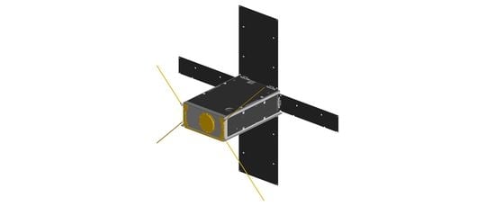
The spacecraft attitude in flight will be stabilized so that the optical line of sight (z-axis in Figure 1a) constantly points towards the Sun. This feature also drives the configuration of the deployable solar panels and the positioning of the star tracker, which requires a clear view to deep space. It also reduces the sensitivity to thermal variations during eclipses and facilitates thermal management of the spacecraft.

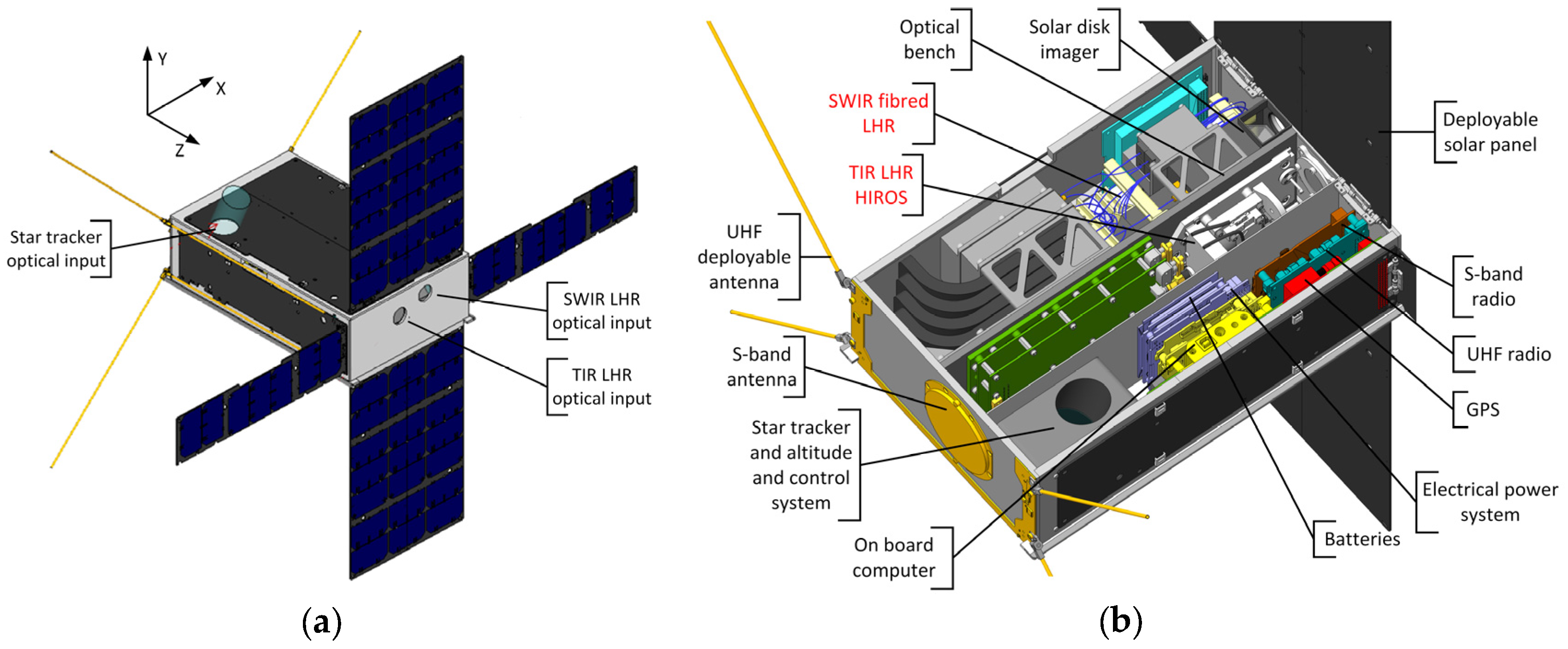
The platform and the two payloads are illustrated in Figure 1b, in which the spacecraft is shown with the top cover removed. The structure is bespoke to allow efficient packaging of the instruments and spacecraft subsystems. The bottom panel, not directly exposed to the Sun, can be used as a radiator, whilst the optical bench is positioned along the (y, z) plane and shared, on either side, by the two instruments. This configuration simplifies the pre-flight co-alignment of the two fields-of-view (FoV) and ensures in-flight stability of their co-registration.

The spacecraft accommodates the SWIR LHR and a solar disk imager, which together occupy ~3U (10 × 10 × 30 cm³) and HIROS (~1.5U or 10 × 5 × 30 cm³). The solar disk imager is embedded within the SWIR LHR optical input port and provides diagnostic data on the pointing knowledge, source strength and information on clouds towards lower tangent heights. The remaining ~1.5U houses the spacecraft subsystems including: (1) the attitude determination and control system, which ensures a pointing accuracy of <0.003° in the x and y axes; (2) the on-board computer; (3) the electrical power system, comprising solar panels generating ~40 W, batteries and power conditioning electronics; and (4) the communication platform, which uses a UHF link for telecommanding and housekeeping telemetry and an S-band link for payload data downlink. The overall mass comes to 10.4 kg including margins.

The baseline plan is to use the ISS as a launch platform and the Canisterized Satellite Dispenser from Planetary System Corporation. The IOD will be restricted to a low-Earth orbit accessible from the ISS. The natural variation in the orbit local time at ascending node ensures a variation of eclipse geolocation, which maximizes the global coverage. Using the ISS orbital parameters and retaining limb occultation eclipses comprised between 5 and 50 km tangent heights, ~1800 occultations are expected over a six-month period.

3.2. TIR LHR (HIROS) Instrument

The requirement to develop a TIR spectrometer capable of spectrally resolving individual Doppler-limited stratospheric absorption lines at a wavelength of ~8 µm, whilst being compatible with nanosatellite volume and mass restrictions, calls for the use of laser heterodyne spectro-radiometry (LHR) operating with TIR quantum cascade lasers as local oscillators. HIROS exploits the heritage from several ground-based LHR prototypes that have been demonstrated in solar occultation mode for several atmospheric constituents, including CH₄ [26,27,28]. Hoffmann et al. [28] provide a wealth of details on the TIR LHR approach and performance, which are directly relevant to HIROS.

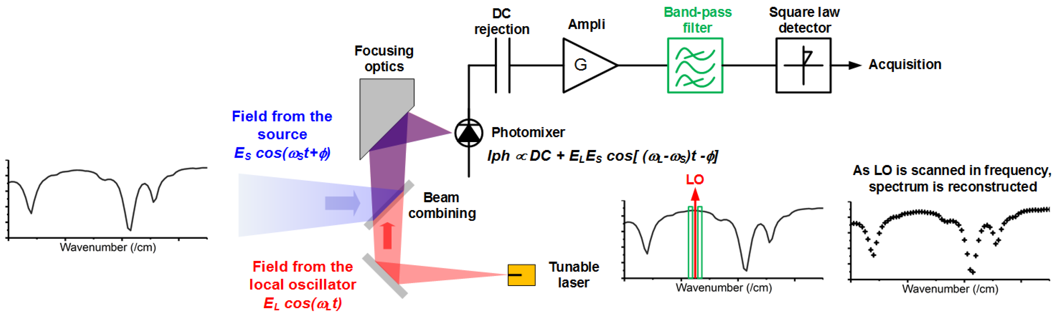
To summarize, the laser heterodyne spectrometry technique relies on optical heterodyne spectral down-conversion, in a similar fashion to heterodyne receivers used in the millimeter wave spectral domain. In the optical domain, the photomixer (the element producing the intermediate frequency (IF)) is a high-speed photodiode, whose response is typically quadratic with respect to the incident electromagnetic field, hence producing non-linear mixing. The implementation of an LHR is illustrated in Figure 2. Incident onto the main collection aperture of the optical system is the radiation one wishes to spectrally characterize. In the case of MISO, this represents the solar radiation that has passed through layers of the atmosphere and therefore contains spectral absorption signatures from atmospheric constituents. This source radiation is mixed with that of an ideal local oscillator (LO), which in the optical domain is well approximated by a single mode laser source. At the photodiode output, once the continuous photocurrent component has been removed, the IF signal contains a continuous spectrum of beat frequencies within the photodiode’s electrical bandwidth. This signal is amplified and further filtered by a low- or band-pass filter. This filter defines the amount of RF power centred around the LO frequency that is transmitted to a Schottky detector (square law detector). It therefore defines the instrument lineshape and the spectral resolution of the LHR. The voltage signal delivered by the Schottky diode is proportional to the LO power and to the broadband signal power within the instrument’s bandwidth as defined by the RF filter. For simplicity, the MISO LHRs retain operation in the LO sweep mode, in which the laser frequency is continuously tuned to sequentially reconstruct the part of the spectrum within the tuning range of the LO.

LHR combines several advantages: (1) ideally a shot noise limited operation, in practice limited by photodiode performance; (2) a very high spectral resolution (>500,000 resolving power), well suited for Doppler-limited and sub-Doppler spectroscopy with lineshape resolution; (3) a very narrow field-of-view defined by the LO divergence properties, which is a coherent source; and (4) a highly stable instrument lineshape defined by an electronic filter.

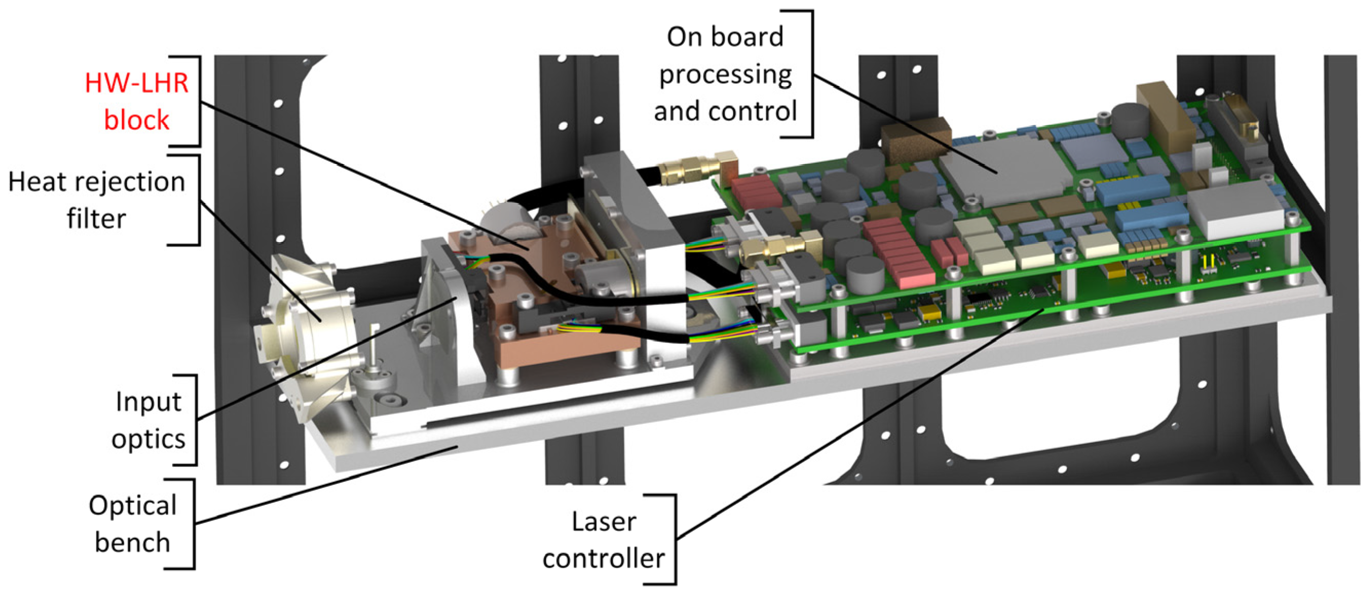
To achieve the level of miniaturization compatible with MISO, the TIR LHR was dramatically miniaturized using full optical integration within a hollow waveguide circuit [29]. As a result, the core of the spectrometer is encapsulated in a monolithic substrate of ~5 × 6 × 2 cm³, which includes the laser, optics and (thermoelectrically cooled) detectors. Figure 3 shows a CAD model of the HIROS instrument with the key component (the hollow waveguide integrated LHR block (HW-LHR)) highlighted in red. The front-end optics, composed of an on-axis, obscured, reflective all-aluminium telescope using a fast primary mirror (25 mm diameter) to limit the obscuration ratio, is coupled to the HW-LHR. The design of the telescope is partly driven by the need to limit the sensitivity of the hollow waveguide input coupling to the telescope alignment. In front of the input aperture, a heat rejection filter allows only the in-band TIR radiation through and rejects (reflects and/or absorbs) the rest of the solar spectrum.

Behind the optical subsystems are two electronics boards. The lower one is dedicated to the quantum cascade laser control (laser current tuning and laser temperature stabilization); the top one provides data acquisition, control, lock-in amplification, local storage and data pre-processing, before sending it to the spacecraft’s on-board computer for subsequent downlink.

3.3. SWIR LHR Instrument

The SWIR instrument is also an LHR, but uses conventional telecom laser and photonic technologies operating at a wavelength of ~1.6 µm. As with the TIR LHR, extensive demonstrations using ground-based prototypes have been made [30,31]. The SWIR LHR within MISO is based on the fully fiber-coupled design described in Rodin et al. [31]. 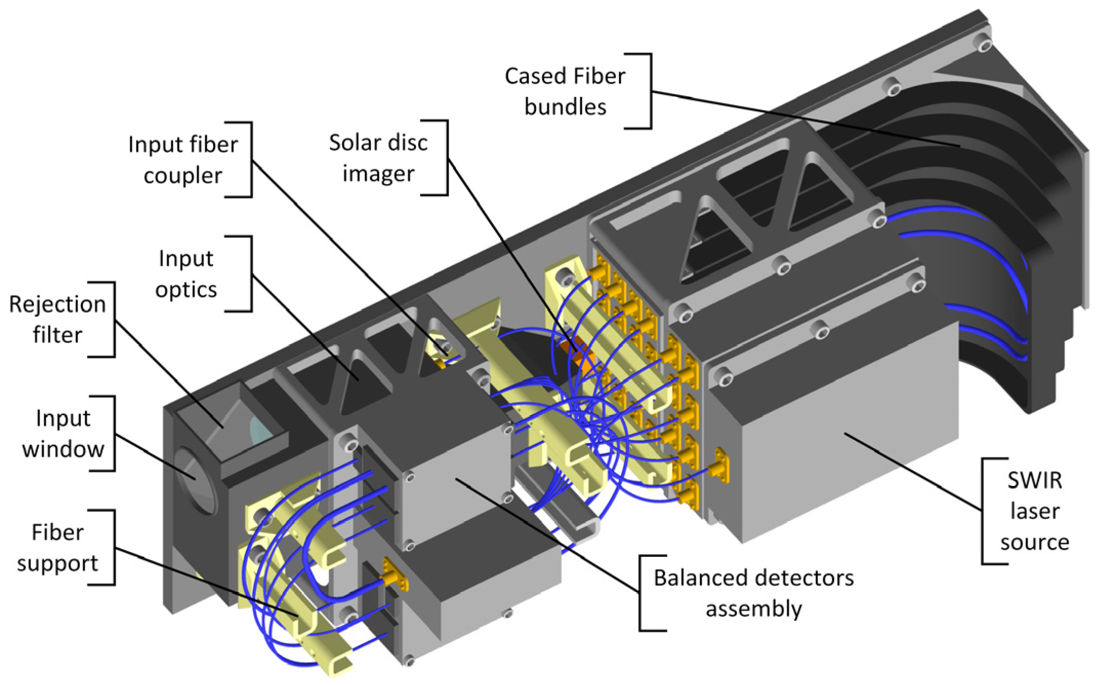In addition, to enhance the SNR and achieve comparable performance to the TIR LHR, the instrument relies on a balanced detection scheme and spatial multiplexing implemented using a multicore fibre input [32]. The solar radiation input is coupled into a seven-core fibre bundle, directed into four balanced detection modules. The front-end coupling optics are merged with the solar disk imager, in which a dichroic beamsplitter is used to separate the SWIR radiation from the visible. Figure 4 shows the 3D CAD model of the SWIR LHR packaged for incorporation into the MISO spacecraft.

4. Spectral Channel Selection

In the MISO implementation, the LHR spectral coverage is determined by the range of the frequency sweep of the local oscillator laser, which is typically in the range of ~1 cm⁻¹, obtained by modulation of the laser drive current. At the same time, the resolving power of the approach allows full lineshape resolution of Doppler-limited lines. This implies that spectral coverage optimization becomes a line-by-line analysis in terms of transition intensities, temperature and pressure dependence, to mention only the first-order parameters that govern the lineshape.

The spectral channel selection for the MISO mission combines three aspects: (1) maximizing the amount of information that can be retrieved from the instrument’s data whilst minimizing interference from other trace gases, for which the concepts of the optimal estimation method (OEM) are used [10]; (2) reducing the methane isotopic ratio sensitivity to atmospheric temperature uncertainties; and (3) taking into account instrumental and mission limitations. This analysis is performed specifically for limb sounding through the UTLS and stratosphere, where the instruments will need to cope with large signal dynamic ranges due to exponential changes in the sounded air mass.

4.1. Observing System Simulator for Information Analysis

To carry out the quantitative analysis on the degrees of freedom for signal (DFS) and the total information content of an atmospheric measurement, an observing system simulator (OSS) made of an atmospheric line-by-line radiative transfer code (the Reference Forward Model (RFM) [33]), an LHR instrument and noise model and an OEM retrieval algorithm have been developed. An updated, improved and more generic version of the OSS already described in Hoffmann et al. [28] has been generated. As part of a complete overhaul of the code, the core of the algorithm has been modified to handle the retrieval of isotopologues as individual species.

The OSS is used to conduct a sliding window analysis, for which solar occultation limb sounding at 9 and 18 km tangent heights is simulated, in relevance to mid-latitude UTLS. The measurement vector is made from appended spectra corresponding to the two tangent heights. For each narrow spectral window (0.5 cm⁻¹), a single iteration is calculated to derive the averaging kernel (AK) matrix, from which DFS and information content are quantified. The diagonal measurement error covariance matrix (S_ε) is populated with a constant variance assuming the ideal case of a shot noise limited LHR. The a priori covariance matrix (S_a) is defined arbitrarily as a diagonal matrix with 50% relative error. The full list of OSS parameter settings is given in

Table 1. Parameters used in the OSS used for sliding window analysis, for a limb observer at 1000 km altitude.

Parameters	Value/Setting
Radiative transfer code	RFM v4.35 patch 117 (run in transmission)
Spectroscopic database	Hitran 2012
Retrieval products	CH4 isotopologue or gas
State vector altitude grid	8.4, 9.4, 10.7, 12.8, 15.6, 17.6, 18.6, 19.9, 22.6, 27.9 km
Atmospheric gas and p, T profiles (truth, prior, first guess)	MIPAS2001 mid-latitude day, FASCODE for CFCs and minor constituents
A priori covariance matrix (Sa)	Diagonal, 50% relative error
Gas species included	H2O, CH4, N2O, CO2, O3, H2O2, COF2, HNO3, HOCl, N2O5, F115, F114, F13
LHR spectral resolution	0.002 cm−1
Instrument lineshape (ILS)	From laboratory measurements
Mixer heterodyne efficiency	0.5
System optical efficiency	0.5
Integration time per sample	50 ms
Source blackbody temperature	5778 K
Window size/sliding step	0.5/0.2 cm−1
Sampling resolution	0.002 cm−1
Tangent heights	9 and 18 km

. The parameters used for the analysis do not define a fully realistic instrumental scenario at this stage, as the focus is on identifying the relative optimum narrow spectral windows to be used for the subsequent full performance analysis, for which instrumental parameters are refined. Sliding window analyses are run separately for all retrieval products of interest (three main CH₄ isotopologues—¹²CH₄, ¹³CH₄ and CH₃D—and CO₂) and for the dominant interfering absorbers (H₂O, O₃, N₂O, HNO₃, and F14), to quantify their respective DFS as a function of frequency. The TIR spectral range covered was set between 1200–1380 cm⁻¹. The 10-layer state vector altitude grid was defined via the cumulative trace method [34].

As a diagnostic metric, a weighted sum of the individual DFS can be constructed according to the mission objectives, which ensures the agility of the approach to alternative mission opportunities. The weighting factor is tuned depending on whether a species is considered as a desired product (+1 weight, for example), or as an interference (−1, for example) that could impede the accuracy of the product’s retrieval. This method still does not account for potential heavy line overlap that may impede selectivity. The preferred window(s) of interest should exhibit a high target species DFS sum and a low contaminant DFS sum. Once such windows are selected, interferences are evaluated both visually and qualitatively.

4.2. Additional Selection Parameters

In the context of isotopic ratio measurements, additional selection parameters can be added, such that individual molecular transition parameters and their dependencies form an integral part of the selection process. Based on the development of tunable laser in-situ isotopic analysers, it had been found that the sensitivity of the isotopic ratio to temperature can constitute a major source of uncertainty when individual lines are used for sensing. Therefore, the window selection ought to take this into account. Following Bergamaschi et al. [35] and Weidmann et al. [36], a first criterion for isotopologue line selection requires similar lower state energies of the ro-vibrational transitions.

Isotopic ratios are usually expressed as a delta value, which represents the relative difference in the isotopic ratio of a sample against that of an established reference. In the case of methane carbon isotopic ratio, this quantity is defined by Equation (1) where δ¹³CH₄ is expressed in per mil (‰) and R_r is the Pee Dee Belemnite standard ratio R_r = 0.0112372.

$${\delta }^{13}{CH}_4=\left(\frac{\left[{}^{13}C{H}_4\right]}{\left[{}^{12}C{H}_4\right]}\cdot \frac{1}{R_r}-1\right)\cdot 1000,$$

(1)

The bias Δδ on the isotopic δ value induced by a temperature bias of ΔT can be expressed by Equation (2), in which ΔE″ is the lower state energy difference between the two isotopic molecular transitions considered, k the Boltzmann constant and T the absolute temperature.

$$\Delta \delta \cong \Delta T\cdot \Delta E^{″}/\left(k\cdot T^2\right),$$

(2)

This equation allows thresholds on the maximum allowable values of Δδ¹³CH₄ and ΔT to be set, which defines a subset of ¹³CH₄ and ¹²CH₄ lines that fulfil the requirement. A temperature of 220 K has been chosen to represent UTLS conditions.

A criterion for line intensities, S, can also be defined. Solar occultation limb measurements over a wide range of altitudes imply a large dynamic range in transmission. Isotopologue line intensities need to be carefully selected to yield a detectable absorption signal and to avoid saturation, whilst allowing measurement over the widest range of altitudes possible for both isotopologues. The maximum line intensity S_max was estimated for a tangent point height of 8 km, where transmission was coarsely modelled as a single gas cell of 1000 km length, containing 2 ppm of CH₄ at 350 mbar total pressure and 235 K temperature. An S_max of 5.0 × 10⁻²² cm⁻¹/(molec cm⁻²) was chosen. Similarly, for S_min, a tangent point height of 24 km was modelled as a single cell of 700 km length, with 1 ppm of CH₄ at 30 mbar total pressure and a temperature of 220 K. The criterion for line strength selection was a transmission of ~0.9. S_min was then set at 1.0 × 10⁻²³ cm⁻¹/(molec cm⁻²). Note that simple gas cell models to approximate limb transmission at tangent height have only been used for the purpose of setting the range of line intensities to consider during the line selection exercise.

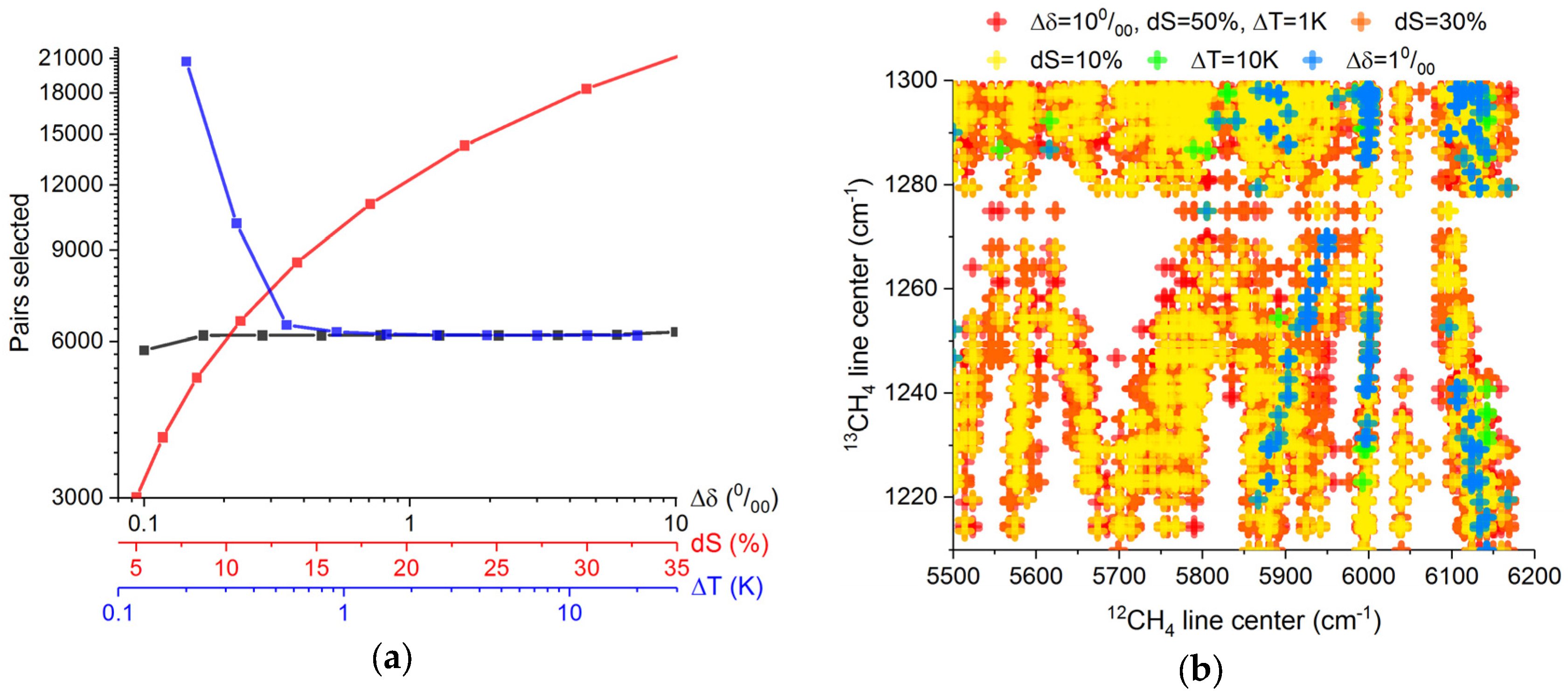
Within this defined range, a further criterion is set to ensure that absorption intensities from the ¹²CH₄ and ¹³CH₄ lines are similar (factoring in the natural abundances), to limit dynamic range and non-linearity issues. This is specified through a maximum acceptable relative intensity difference (dS) between the two isotopic lines. While this method does not account for the combined effect of multiple overlapping or densely-spaced lines, it offers a good first filter for setting line selection parameters.

The sensitivity to the different selection criteria has been evaluated by monitoring the number of relevant line pairs as the criteria are made more stringent. Only the two most abundant isotopologues, ¹²CH₄ and ¹³CH₄, have been considered. The outcome is plotted in Figure 5a, where only pairs with ¹³CH₄ transitions in the 500–1500 cm⁻¹ range have been retained. Sensitivity to the temperature uncertainty (ΔT) is the primary one to consider, given that the sounded air mass temperature error is likely to be a significant source of bias. Temperature uncertainties throughout the atmospheric profiles of a few Kelvin are to be anticipated. The selection is quite sensitive to the relative intensity difference, dS, and this criterion can be relaxed to higher values to increase the likelihood of finding suitable line pairs.

The wavelength range of suitable line pairs also relates to the spectrometer technologies to be used. Figure 5b shows identified pairs and their relative wavenumber positions for a number of selection criteria. HIROS has been set to operate in the fundamental ν₄ CH₄ band in the 1200–1250 cm⁻¹ range, to maximize the SNR. Shortwave of 1250 cm⁻¹, the atmosphere becomes optically thick at low tangent heights. The SWIR instrument draws on telecom laser technology and targets the CH₄ 2ν₃ overtone band at ~5850–6150 cm⁻¹, where most of the transitions selected with the baseline parameters reside (blue crosses in Figure 5b). The selection of the dual SWIR/TIR co-registered sounding for MISO originates from the preceding isotopic ratio line selection criteria.

4.3. Selected Spectral Windows

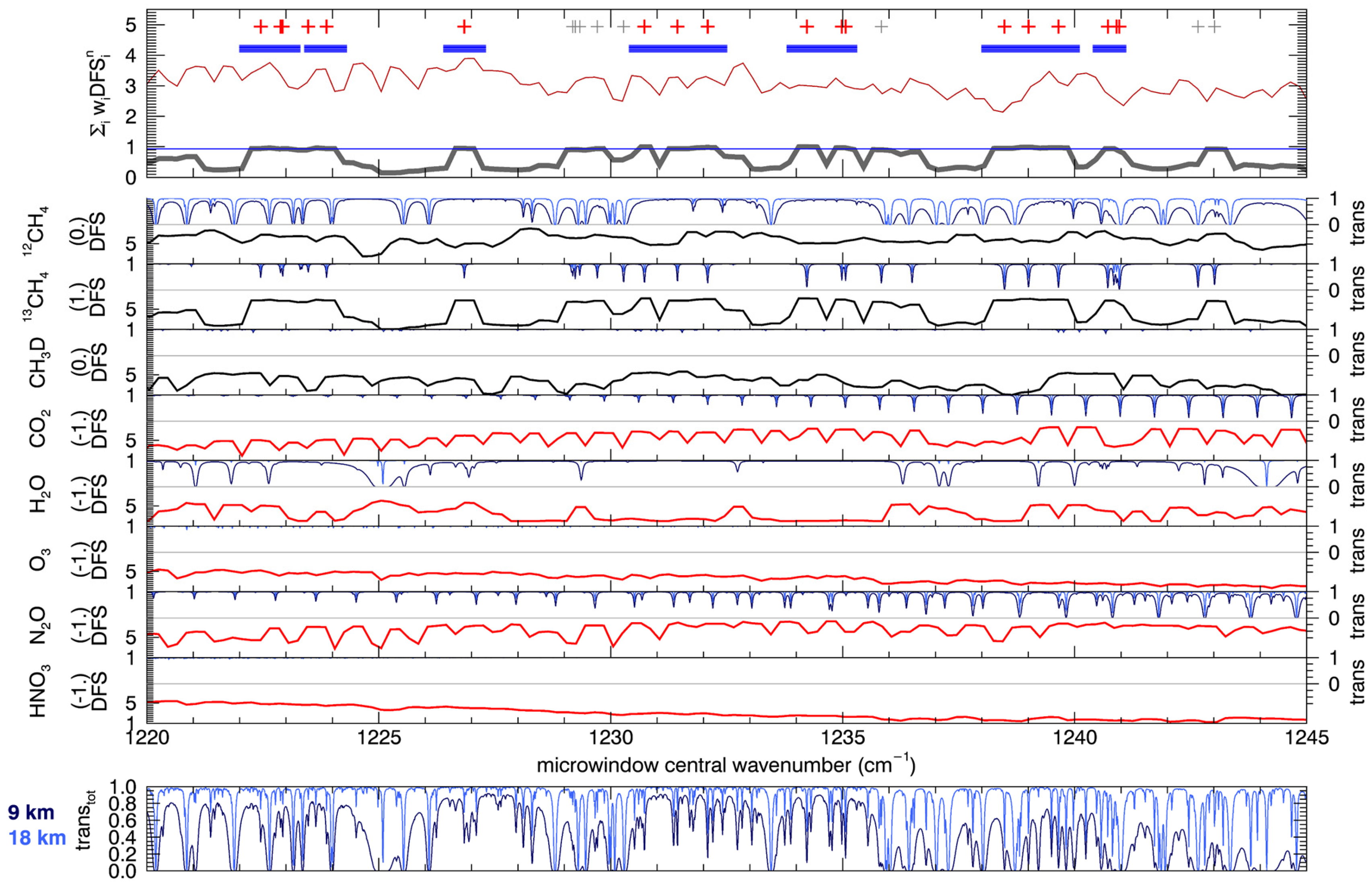
The combination of DFS analysis and isotopic line selection criteria is illustrated in Figure 6 for the case of HIROS channel selection, with only a subset of the wavelength range shown for clarity. From bottom to top, the following panels are shown: (1) the simulated atmospheric transmission at 9 and 18 km tangent heights; (2) five panels with individual DFS and transmission contributions for interfering species and CO₂; (3) three panels with individual DFS and transmission contributions for potential products (¹³CH₄, ¹²CH₄, CH₃D) and (4) the aggregated product DFS and interfering species DFS along with an indication of lines fulfilling the isotopic selection rules.

The top panel in Figure 6 summarizes the selection. The weighted product DFS sum (black line) provides the selection metric ensuring the maximum information on methane isotopologue is retrieved. By setting an appropriate but arbitrary threshold, spectral intervals of interest are automatically determined. Within these intervals, the individual isotopic lines fulfilling the criteria described in the previous section are retained for further scrutiny. These are highlighted as red crosses in the graph. At the same time, a low interfering species DFS (red line) is preferred. Since DFS is a metric characterizing the full narrow window and does not provide any information of the transition’s centre frequency, the interfering species DFS is only indicative for the selection. The potential candidates are thus further vetted by taking into account qualitative inspections of potential line overlaps and cross-talk.

Lastly, the limitations of the SWIR photodiode used in the SWIR LHR are considered. This device exhibits a sensitivity drop below 6000 cm⁻¹, detrimental to the SWIR LHR SNR. Limiting the detector responsivity drop to ~15% from its maximum value implies that the SWIR line must be at frequencies >5990 cm⁻¹.

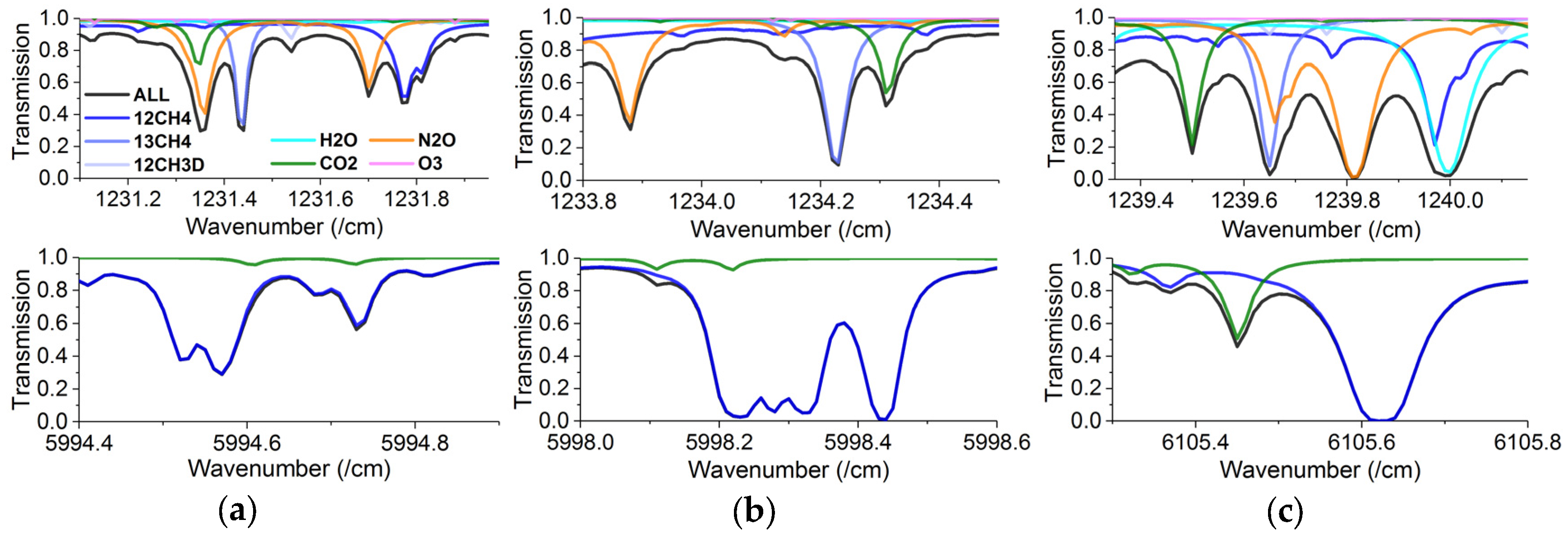
Three interesting candidates, shown in Figure 7, are retained, for which the following selection criteria are met: dS < 80% and Δδ < 5‰, for ΔT < 5 K. Two of the three selected channels (Figure 7a,b) are close enough in frequency that they could potentially be selected in orbit by modification of the laser temperature operating point. The pair from Figure 7a includes additional information about CH₃D, which would significantly enhance the isotopologue characterization. Aggregated CO₂ and N₂O information is also available. The pair in Figure 7b would ensure better SWIR detector response and include a strong CO₂ signal (¹⁸OCO). The pair in Figure 7c contains additional information on CO₂, N₂O and also H₂O, which is very relevant to the study of CH₄/H₂O interactions in the stratosphere. However, the overlapping absorption lines may lead to an increase in cross-talk.

The case of Figure 7b has been retained for the following performance and sensitivity analyses. The TIR spectral window was set to 1234.25 ± 0.15 cm⁻¹ and the SWIR one to 5998.30 ± 0.30 cm⁻¹. The SWIR window actually harbours eight ¹²CH₄ lines with similar lower state energies to the ¹³CH₄ TIR transition (<0.2 cm⁻¹ difference). Most of the lines satisfy dS < 40%.

5. Preliminary Performance Analysis

The preceding channel optimization aimed to determine the relative amount of information to discriminate between spectral windows. The analysis was performed for instrumental parameters settings not necessarily realistic of the mission, particularly as far as integration times are concerned. For the performance analysis, optimized instrumental parameters are refined and trade-offs made as required.

5.1. Instrumental and Atmospheric Parameter Definition

Firstly, the spectral resolution is considered. With LHR technology, the spectral resolution is defined in the electronic domain, usually using low-pass filters or equivalent processing. With the very high spectral resolution achievable by LHR, it is possible to probe well-defined individual absorption lines in the upper atmosphere, where Doppler broadening overwhelmingly dominates the observed linewidths. At a representative UTLS temperature of 220 K, Doppler broadening of CH₄ (full width at half maximum (FWHM)) is ~100 MHz (0.0033 cm⁻¹) and ~480 MHz (0.016 cm⁻¹) at 1250 and 6000 cm⁻¹ respectively. A spectrometer spectral resolution of the order of the Doppler FWHM ensures the best compromise between lineshape resolution and absorption sensitivity. A closer analysis of DFS as a function of the spectral resolution, holding the total measurement time constant by changing the integration time per spectral sample, shows that resolutions of 120 MHz and 200 MHz are well suited for HIROS and the SWIR LHR, respectively. The spectrometers’ spectral resolutions are modelled by synthetic top hat instrument lineshape functions of the selected spectral widths.

The second parameter driving instrumental performance is the number of sampling points per spectrum and the integration time per sampling point (τ), both of which drive the total time required to acquire one spectrum. HIROS and the SWIR LHR operate in a local oscillator sweep mode, which means that spectra are sequentially acquired, whilst the laser frequency is scanned across the selected narrow spectral window. For simplicity, the sampling resolution is set to be equal to the spectral resolution. The acquisition time to obtain a full spectrum also relates to the vertical resolution achieved in limb sounding because of the tangent point descent/ascent rate for a fixed sounding line-of-sight, proportional to spacecraft velocity. For an orbit altitude of 400 km, this rate is ~2.5 km/s, discarding atmospheric refraction and assuming an orbital plane containing the Sun (zero beta angle). Ignoring the instrument FoV function in the performance analysis, the acquisition parameters have been constrained by: (1) the spectral resolution as defined in the previous paragraph; and (2) a desired sounding vertical resolution (measurement spacing) of 2 km, which implies recording a full spectrum approximately every 800 ms and yields integration times per spectral sampling point of the order of 10 ms.

For limb sounding, the information collected comes primarily from the atmospheric layer corresponding to the tangent height. A 2 km vertical grid was therefore used for the retrieval, spanning 8–54 km and coinciding approximately with the measurement tangent points.

As part of the analysis, the “true” atmospheric state to be used in the OSS and against which the retrieval will be compared, needs to be defined, particularly as far ¹²CH₄ and ¹³CH₄ profiles are concerned. Profiles have been constructed from a number of sources. The tropospheric (<8 km) concentration for total methane has been set to a constant value. From 8 km to 29 km, data from the GAP-99-06 balloon-borne in-situ measurements found in [21] have been used. Between 29 km and 50 km, the SCISAT-ACE-averaged profile from [16] was used. Finally, above 50 km, the standard MIPAS 2001 mid latitude day profile was used.

For the δ¹³CH₄ profile, data from the Whole Atmospheric Community Climate Model (WACCM) found in [24] have been used to complement the balloon campaign data from [21] both in the troposphere and above 29 km. The constructed ¹²CH₄ and ¹³CH₄ profiles were given some further random fine-scale structure and then scaled to compensate for the fact that line intensities in Hitran 2012 include a natural abundance correction factor.

5.2. Instrument Error Propagation—Precision

Full OSS retrievals based on a Levenberg–Marquardt solver have been run over 50 members for both HIROS and the SWIR LHR in order to produce ensemble results on which statistical analysis can be done to validate the OEM error propagation. Only the random noise seed added to the synthetic “measured” spectra varies between runs. For each instrument, the measurement vector is composed of 24 concatenated spectra measured over increasing tangent heights. A priori data for the CH₄ profile were set to the MIPAS 2001 mid-latitude day profile and the ¹³CH₄ a priori profile was such that δ¹³CH₄ remains a constant profile at ~0‰.

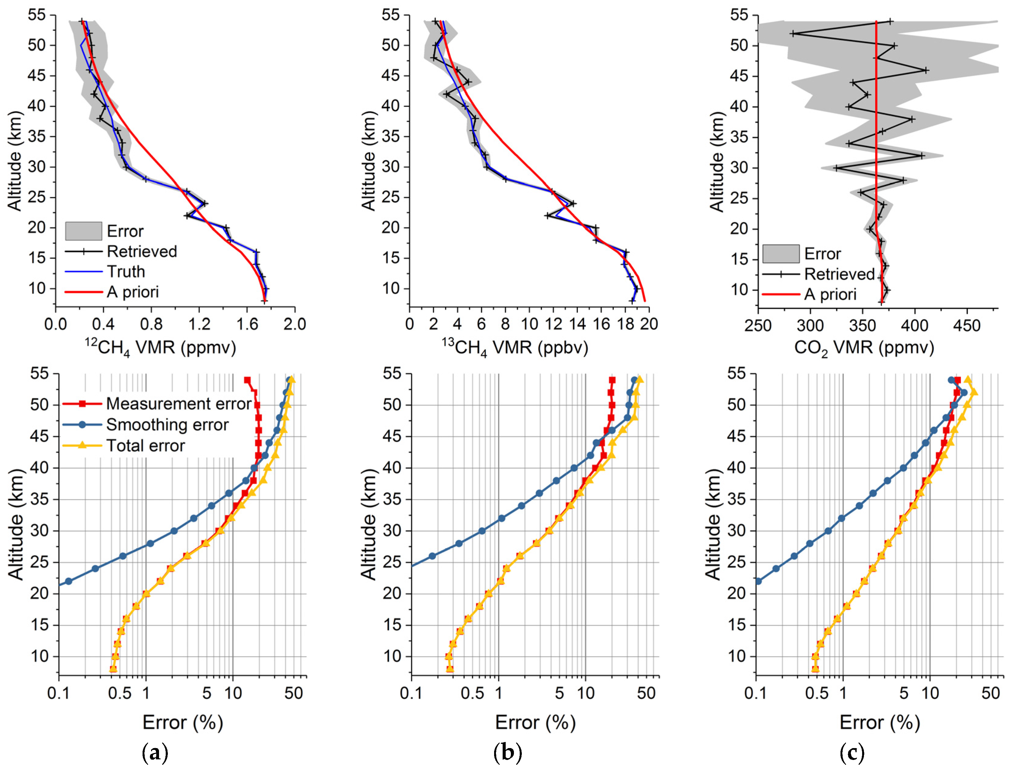
The outcome from one observation simulated for ideal instruments at the shot noise limit is shown in Figure 8, in which Figure 8a refers to ¹²CH₄ retrieved from SWIR LHR, Figure 8b to ¹³CH₄ retrieved from HIROS and Figure 8c to CO₂ retrieved from HIROS. As expected in the case of solar occultation limb sounding with high SNR (~780 for HIROS, ~250 for SWIR LHR; see, e.g., Equation (10) in [28], the value for the SWIR LHR has further been multiplied by $\sqrt{7}$ to account for the 7 fibres), the averaging kernels (AK) are nearly ideal. Considering a threshold of AK > 0.5, a single observation can provide sensitivity up to ~44, ~48 and >50 km for ¹²CH₄, ¹³CH₄ and CO₂, respectively. The TIR retrieval brings a total information content of 215 bits and a total DFS of 44 (2 species retrieved); the SWIR retrieval brings 99 bits of information and a DFS of 20 (1 species retrieved). The error bars from the OEM error propagation, denoting the aggregated measurement and smoothing error, match those derived from the ensemble statistics well. On the methane retrieved profiles, the vertical structures of the “truth” interpolated over the retrieval grid are well reproduced.

This single occultation in ideal instrumental conditions (shot noise limited detection and no broadband or continuum absorption contribution) provides, owing to the bright background source, a precision <1% in the mid-latitude upper troposphere and <~10% up to 32 (37) km for ¹²CH₄ (¹³CH₄). Note that these retrievals were carried out in sequence for the two isotopologues in question and not using a TIR/SWIR composite measurement vector.

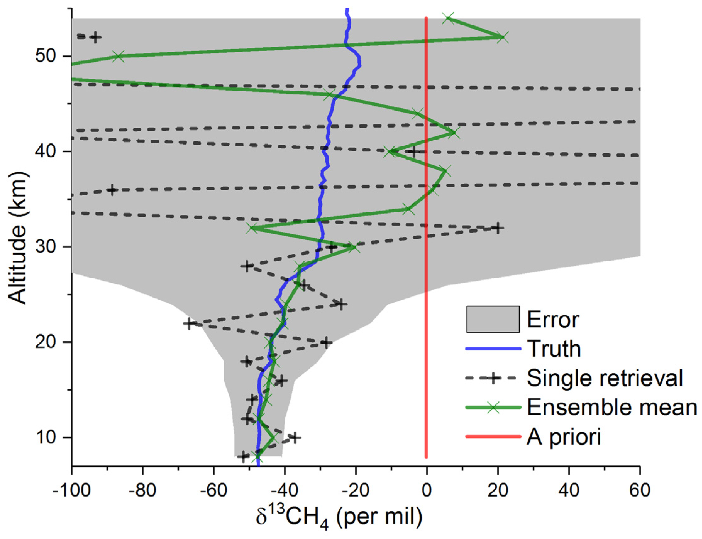
Using Equation (1), a standard error propagation calculation yields Equation (3), which is used to derive the expected error on the delta value. Note that this approach is truly a worst-case scenario, as the standard sum of error is used rather that the root-sum-square.

$$\Delta \delta {}^{13}C{H}_4=\frac{1000}{R_r\cdot \left[{}^{12}C{H}_4\right]}\cdot \left(\Delta \left[{}^{13}C{H}_4\right]+\frac{\left[{}^{13}C{H}_4\right]\cdot \Delta \left[{}^{12}C{H}_4\right]}{\left[{}^{12}C{H}_4\right]}\right),$$

(3)

Combining the data from Figure 8a,b and the instrument error propagated using Equation (3) yields the vertical profile of δ¹³CH₄ shown in Figure 9. The retrieved profile reproduces the truth within the one-sigma error. The error starts at ~7‰ at 8 km and becomes >20‰ for altitudes >21 km for a single occultation. Assuming insignificant isotopic ratio variability over a set of 50 consecutive occultations within a similar geographical area, the precision on δ¹³CH₄ could be brought down to ~1‰ at 8 km through averaging. Alternatively, the retrieval could be improved by using a form of regularization, such as the Tikhonov approach [37].

The single measurements simulated via the OSS as shown above are ideal. In practice, measurement noise is highly likely to be larger compared to the ideal case. When taking into account laboratory measurements using similar photodiodes as those planned for HIROS, at best instrument noise levels five times greater than the ideal shot noise limit are to be expected [29]. In the worst-case scenario, a degradation of ~10 from the ideal case would bring the random instrument noise on recorded spectra on par with those observed using ACE [24]. Assuming linear propagation, this multiplication factor relevant to non-ideal cases applies to the retrieval errors (when the measurement error dominates retrieval errors). As mentioned above as a numerical example, error reduction can always be obtained through temporal and/or zonal averaging, assuming limited temporal or spatial variability of the upper atmospheric isotopic ratios.

5.3. Elements of Systematic Error Analysis—Accuracy

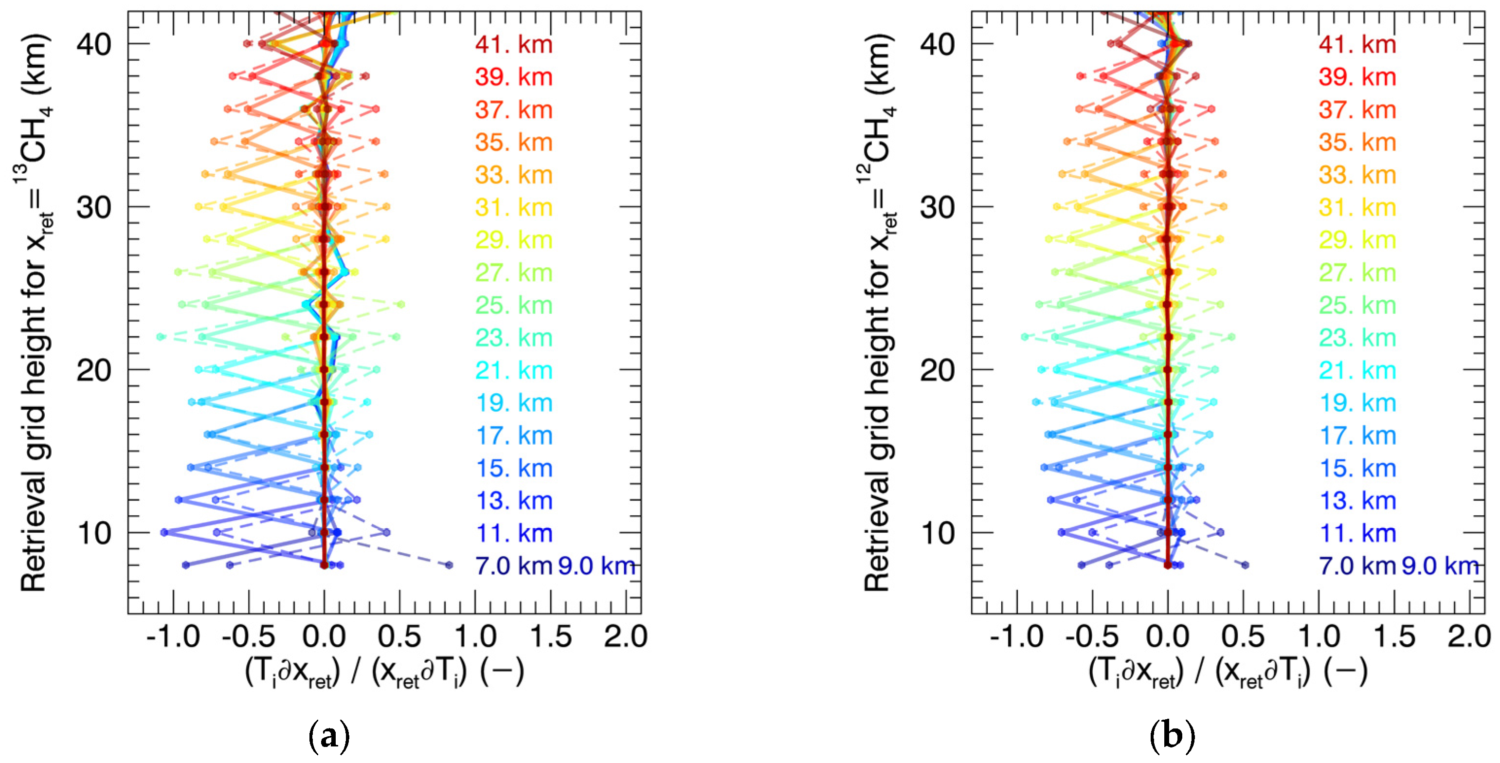
Whilst random measurement errors need to be considered to determine the feasibility of the mission, other sources of (systematic) errors will contribute and dominate the accuracy budget. Sources of systematic errors are numerous and their full study is beyond the scope of this initial spectral selection and assessment of MISO’s feasibility. As a first step, insights into the sensitivity of retrieved profiles to pressure and temperature perturbations have been investigated.

The most straightforward (though computationally expensive) approach to estimate retrieval sensitivity to temperature and pressure perturbations has been employed. The retrieved state $\widehat{\mathit{x}}$ can be written as the result of a retrieval function, R, as shown in Equation (4), applied to four sets of parameters. Vector y represents the measured data, x_a represents the a priori data, $\widehat{\mathit{b}}$ is a best estimate of all the other physical parameters required for the forward function (pressure and temperature profiles fall within this category) and c includes additional retrieval method parameters (e.g., convergence criteria, damping, scaling, interpolation, etc.).

The direct estimation of retrieval sensitivity to a model parameter $\widehat{\mathit{b}}$ is given by Equation (5). Practically, this evaluation is run by artificially scaling down the measurement error by three orders of magnitude to render it insignificant and perturbing temperature and pressure values by 1% at each 1 km level sequentially. G_b is then normalized to be expressed in terms of relative errors. In the case of solar occultation limb sounding, the outcome is quasi-diagonal, reflecting the vertical sensitivity of the measurement. The example in the case of temperature sensitivity is shown in Figure 10.

$$\widehat{\mathit{x}}=\mathit{R}\left(\mathit{y},\widehat{\mathit{b}},{\mathit{x}}_{\mathit{a}},\mathit{c}\right),$$

(4)

$${\mathbf{G}}_{\mathbf{b}}=\frac{\partial \widehat{\mathit{x}}}{\partial \widehat{\mathit{b}}}=\frac{\partial \mathit{R}}{\partial \widehat{\mathit{b}}}\cong \frac{\mathit{R}\left(\mathit{y},\widehat{\mathit{b}}+\Delta \widehat{\mathit{b}},{\mathit{x}}_{\mathit{a}},\mathit{c}\right)-\mathit{R}\left(\mathit{y},\widehat{\mathit{b}},{\mathit{x}}_{\mathit{a}},\mathit{c}\right)}{\Delta \widehat{\mathit{b}}}$$

(5)

Quantitatively, the largest sensitivity is to temperature around the tropopause, where a 1% relative uncertainty in temperature (~2 K) will result in a ~1% uncertainty in the retrieved CH₄ isotopologues volume mixing ratios (VMR). The sensitivity is negative as expected from a ro-vibrational transition whose strength increases with a temperature increase, requiring an under-estimation of the number density. The sensitivity is actually larger (~2%) on molecular number densities, as the VMR sensitivity is slightly offset by the p, T perturbations on the total air molecular number density. Whilst the temperature bias affects the individual isotopologue mixing ratio retrievals, as per the optimized spectral window selection, a 5 K bias maintains the delta value within the limit of the measurement error.

Sensitivity to pressure perturbations is similar if expressed in terms of retrieved VMRs, where the sensitivity is almost entirely due to the change in total air molecular number density. Corrected for this effect, the relative uncertainty in retrieved gas number densities for a 1% change in p would be <0.5%. A more in-depth assessment will be necessary in the case of joint pressure retrievals using the CO₂ transition, the error of which would then be correlated with the measurement error.

These data are preliminary and systematic error propagation will fall into the remit of a follow-on phase of full mission definition. The recent results obtained from SCISAT-ACE provide an encouraging precedent for high spectral resolution solar occultation limb sounders, especially as far as isotopic information is concerned. The fundamentally different approach of LHR spectroscopy nevertheless calls for a more in-depth error budget analysis, which could be supplemented by actual data from the IOD. Aspects to be considered for the future mission definition phase include:

• ILS knowledge and stability: Unlike FTS and grating spectrometers, the ILS of LHR is defined by the RF detection chain and, in the standard case, by the response function of the RF low-pass or band-pass filter defining the spectral bandwidth. Errors associated with ILS knowledge and errors (offset, skew or spread) are expected to be insignificant.
• Baseline errors: In the narrow spectral windows, broadband absorption contributions are assumed to produce a flat absorption continuum. In addition, laser power modulation during the laser frequency sweep results in a baseline variation. The impact of these baseline effects on the error budget needs be understood.
• Spectroscopic model errors such as molecular transition parameters or non-local thermodynamic equilibrium (NLTE) effects that are not captured by the model. The use of an extremely narrow spectral window focusing on well-identified absorption lines should favour better control over the model errors. Buzan et al. [24] report that spectroscopic parameter errors were the dominant source of bias in their ¹³CH₄/¹²CH₄ measurements from ACE data.
• Straylight errors: The straylight analysis performed on the optical instrument model suggests these to be insignificant and in the worst case to remain below 0.01% of the radiometric signal, owing to the spatially coherent nature of laser heterodyne detection.
• Spectrally interfering species: The high spectral resolution of LHR turns into high spectral selectivity, which should minimize the impact, as does a judicious prior window selection.
• Spectral calibration: The current engineering baseline is to use monolithic etalons providing a spectral calibration of the order of the sampling resolution.
• Spectral sample correlation: Thus far, spectral samples have been assumed to be uncorrelated. Both experimentally and by using the OSS, the impact of such correlations onto the error budget needs to be understood.
• Radiometric response errors such as offset, gain and non-linearity: In solar occultation, the use of transmittance minimizes sources of radiometric errors. High altitude occultation also provides a direct means of transmittance calibration.
• Knowledge of the FoV function, atmospheric spatio-temporal heterogeneities, vertical correlations and impact of the retrieval grid determination.
• Pointing errors and stability, SWIR/TIR co-registration errors, refraction effects and geo-localization errors.

The bias full analysis will further refine the mission definition and may affect the channel selection and distribution between HIROS and the SWIR LHR.

6. Conclusions

The concept of the MISO nanosatellite IOD mission has been introduced and presented with emphasis on the spectral narrow window selection and a first evaluation of sounding precision through random instrumental noise propagation. MISO exploits miniaturized LHR technology in the SWIR and the TIR that allows a focus on <1 cm⁻¹ spectral windows at very high spectral resolution, suitable for Doppler-limited line-by-line spectroscopy. A specific atmospheric line selection strategy and algorithm for optimization of methane isotopologues sounding has been developed to limit the impact of temperature biases on isotopic ratio measurements. Coupled to a forward model and a retrieval scheme, instrument random error propagation has been carried out for an initial evaluation of MISO’s expected performance.

The ideal performance is found to be outstanding, considering a 6U spacecraft with a mass of ~10 kg. Assuming that LHR is only limited by shot noise and a 2 km spacing vertical grid is used, a single occultation results, in the case of HIROS, in a precision of <1% for altitudes 8–20 km, <5% for 20–30 km and <10% up to 37 km on the methane isotopologue profile. These numbers relate to the best-case scenario; excess random noise and systematic errors are likely to dominate the error budget. However, this early outcome, along with the underlying engineering feasibility study, indicates that MISO is highly likely to achieve its IOD mission objectives.

The combination of miniaturization, low-cost and a fast development cycle, whilst maintaining a high level of performance, makes the MISO approach appealing for high spectral resolution sounding. With versatility in mind, the line selection algorithm has been developed to reconfigure the instruments quickly to achieve other mission objectives and to target different atmospheric species. This makes MISO agile and suitable either as a hosted or as a secondary payload.

Beyond the IOD, MISO is a first step towards a nanosatellite constellation obviating the limited coverage that reduces the utility of solar occultation measurements from a single spacecraft. In addition to starting the development of MISO hardware, further studies to quantify the benefits of MISO within the existing and forthcoming methane observing infrastructure, particularly as far as the estimation of regional methane fluxes is concerned, are needed to refine the early mission definition.