Nonnegative Matrix Factorization With Data-Guided Constraints For Hyperspectral Unmixing


1
College of Electrical Engineering, Zhejiang University, No.38, Zheda Road, Xihu District, Hangzhou 310027, China
2
School of Computer Science, Hangzhou Dianzi University, Hangzhou 310018, China
*
Author to whom correspondence should be addressed.
Remote Sens. 2017, 9(10), 1074; https://doi.org/10.3390/rs9101074
Submission received: 7 August 2017
/
Revised: 16 October 2017
/
Accepted: 18 October 2017
/
Published: 21 October 2017
(This article belongs to the Special Issue Hyperspectral Imaging and Applications)
Abstract
:Hyperspectral unmixing aims to estimate a set of endmembers and corresponding abundances in pixels. Nonnegative matrix factorization (NMF) and its extensions with various constraints have been widely applied to hyperspectral unmixing. L1/2 and L2 regularizers can be added to NMF to enforce sparseness and evenness, respectively. In practice, a region in a hyperspectral image may possess different sparsity levels across locations. The problem remains as to how to impose constraints accordingly when the level of sparsity varies. We propose a novel nonnegative matrix factorization with data-guided constraints (DGC-NMF). The DGC-NMF imposes on the unknown abundance vector of each pixel with either an L1/2 constraint or an L2 constraint according to its estimated mixture level. Experiments on the synthetic data and real hyperspectral data validate the proposed algorithm.
1. Introduction
Hyperspectral data consists of hundreds of contiguous narrow spectral bands and has been widely used in many fields [1]. Due to the limitation of the sensor’s spatial resolution, there exist mixed pixels consisting of several material signatures. To address this problem, hyperspectral unmixing (HU) has been adopted to decompose mixed pixels into endmember signatures and their corresponding proportions. According to the availablity of the prior knowledge, HU methods can be divided into three categories: unsupervised [2,3,4,5], semisupervised [6], and supervised [7] methods. We can also categorize HU methods into geometric methods and statistical methods. The pixel purity index (PPI) [8], N-FINDR [9], vertex component analysis (VCA) [10] and the simplex growing algorithm (SGA) [11] are the most famous geometric methods. The relationships among these methods are explored in [12,13,14]. There are also many statistical methods for hyperspectral unmixing [15,16,17]. Nonnegative matrix factorization (NMF) [18] is a typical statistical method [19]. It has been shown to be promising in extracting sparse and interpretable representations from a data matrix. The NMF decomposes a data matrix into two low-rank matrices with nonnegative constraint [20]. The decomposition results of NMF consist of a basis matrix and a coefficient matrix, which provide an intuitive and interpretable representation of data. As an unsupervised method, NMF is applied to hyperspectral unmixing and shows its advantages in many situations. To reduce the solution space, constraints on endmembers [21,22,23,24] and abundances [25,26] have been exploited and used in NMF. Recently, a sparseness constraint has been added to NMF to generate unique solutions and leads to better results [25,27]. The constraint is a widely-used sparseness constraint. However, regularization has the limitation that it cannot enforce further sparseness when the abundance sum-to-one constraint is used. The constraint is representative of . The solution of the regularizer is sparser compared with that of the regularizer. However, the regularizer also brings nonconvexity to the optimization problem. The nonconvex optimization problem with the regularizer can be solved by transforming the regularizer into a series of convex weighted regularizers [28]. -NMF is a popular NMF regularization method [29]. The authors have shown that the regularizer can overcome the limitation of the regularizer and enforce a sufficiently sparse solution. On the contrary, -NMF generates smooth results rather than sparse results [30]. In [31], piecewise smooth nonsmooth (PSnsNMF) and piecewise smooth NMF with sparseness constraints (PSNMFSC) are proposed by incorporating the piecewise smoothness of spectral data and sparseness of endmember abundances. The authors of [32] propose NMF with sparseness and smoothness constraints (NMFSSC). However, NMFSSC does not consider the sparsity level of data and just imposes sparseness and smoothness constraints simultaneously. In data-guided sparsity-regularized nonnegative matrix factorization (DgS-NMF) [33], the sudden change areas are assumed to be highly mixed and a heuristic method is proposed to employ the spatial similarity to learn the mixed level in the hyperspectral images. The pixel with a higher sparsity level corresponds to a sparser constraint (from the norm to the norm). In [34], a learning-based sparsity method is proposed to learn a guidance map from the unmixing results and impose an adaptive -constraint.
In this paper, we propose a nonnegative matrix factorization with data-guided constraints (DGC-NMF). Unlike traditional constrained NMF methods that impose the same constraint over entire data, DGC-NMF firstly evaluates the sparsity level of each pixels’ abundances and then decides which kind of constraint should be imposed on the abundances of a pixel adaptively. In real hyperspectral images, the sparsity levels of the pixels’ abundances are varied and the pixels do not necessarily possess spatial dependence with their neighboring pixels. To preserve the distinctive sparsity information of each pixel’s abundances, the sparsity levels of pixels can be learnt via an NMF unmixing process without any sparseness constraint imposed. Therefore, each pixel’s abundances could enjoy a individual constraint according to its sparsity level in our method. In evenly mixed areas, the sparseness constraint may not contribute to achieving a smooth abundance vector of a pixel. Therefore, we also introduce the constraint to reduce extreme abundance values and promote the evenness of pixels’ abundance vector. Whether an constraint or an constraint is imposed on a pixel is learnt from its abundances’ sparsity level. In this way, our method could adaptively enforce sparse or smooth abundance results in regions with different mixed levels. The experimental results of synthetic and real data demonstrate the effectiveness of DGC-NMF.
The main contributions of this paper include two aspects. Firstly, we provide a method to evaluate the sparsity level of data in different areas and obtain the sparseness map of data. The effectiveness of this method has been verified using data with various sparsity levels. Secondly, we propose a novel NMF method which makes use of the sparsity information from data and adaptively imposes constraints according to the mixed levels of pixels. We analyze the sparsity behaviors of NMF with different regularizations and indicate that NMF with fixed constraints may be not applicable for a hyperspectral image with various sparsity levels, while it has been proven that the proposed DGC-NMF is capable.
The remainder of this paper is organized as follows. Section 2 gives a brief introduction of the NMF algorithm and the NMF with the or the constraint. Section 3 presents the proposed DGC-NMF and provides the proof that the objective decreases along the iterates of the algorithm. Section 4 validates the effectiveness of the proposed method on synthetic data and real hyperspectral images. Finally, Section 5 concludes this paper.
2. Preliminaries
2.1. NMF
Consider the hyperspectral image data , where and N is the number of pixels. In the linear mixing model, the hyperspectral data X could be represented as:
where denotes the endmember matrix, denotes the abundances of respective endmembers, and E is a residual term. The NMF algorithm is designed to find an approximate factorization of X, such that , where and . To quantify the quality of the approximate factorization, the Euclidean distance is commonly used to measure the distance between X and . The loss function of NMF based on the Euclidean distance is defined as follows:
where is the Frobenius norm. The problem of NMF is globally nonconvex. The problem is convex for one of the two blocks of variables only when the other is fixed. Estimating the values of W or H is a convex optimization problem when the other is fixed. A multiplication update rule for standard NMF algorithm is presented in [18] to locally minimize the cost function in (2)
where .* and ./ denote element-wise multiplication and division, respectively.
2.2. NMF with Sparseness Constraints
2.2.1. -NMF
Sparsity is an inherent property of hyperspectral data. To reduce the solution space and derive results with expected sparsity levels, some sparseness regularizations are added to constrain the sparseness of abundances. The regularizer is popular for generating sparse solutions. However, the regularizer may not enforce a sufficiently sparse solution while preserving the additivity constraint over the abundances since the sum-to-one constraint is a fixed norm. In [35], Qian et al. propose the -NMF, based on the regularizer. The regularizer possesses two advantages over the regularizer. It can still enforce sparsity with the full additivity constraint imposed. Another advantage is that the regularizer can obtain sparser solutions than the regularizer does [36]. The model of NMF with the regularizer is as follows: [35]
where
and denotes the -th element of H.
The objective in (5) is nonincreasing under the multiplicative update rules:
where denotes the reciprocal element-wise square root for each element in H.
2.2.2. -NMF
Due to the needs of application, the constraint can be adopted to generate smooth results other than sparse results. For areas in hyperspectral images that are evenly mixed with signatures, we also need the regularizer to promote evenness in the abundances of pixels in these areas. In [30], Pauca et al. explore the use of regularizer in NMF algorithm. The cost function with regularization term is expressed as:
where .
3. Proposed NMF with Data-Guided Constraints for Hyperspectral Unmixing
3.1. Sparsity Analysis
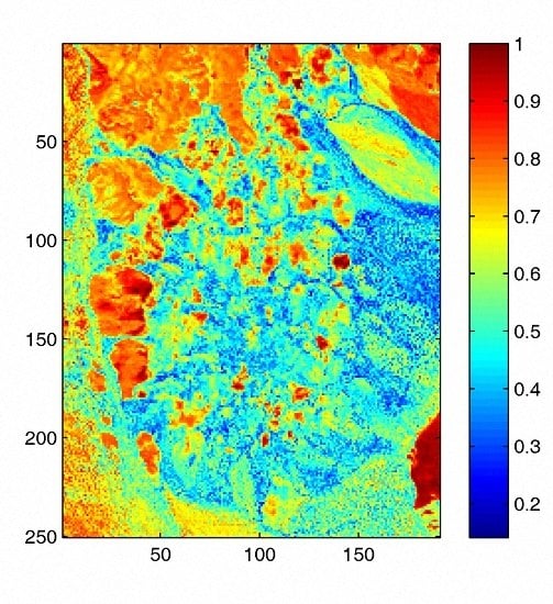
The phenomena of sparsity in abundances commonly exists in hyperspectral images [31]. Sparsity is an inherent property which refers to a representative occasion where mixed pixels could be represented by a few endmember signatures. Accordingly, sparseness constraints such as the regularizer help to obtain unique solutions and lead to better answers in scenes with obvious sparsity. However, in hyperspectral images there exist pixels located in transition regions which are evenly mixed and own low sparsity levels. Imposing a sparseness constraint over the entire image may not contribute to the unmixing accuracy of those evenly mixed pixels. Therefore, we also adopt an regularizer to promote the evenness of pixels’ abundance vectors, achieving an effect on abundances opposite to that of the regularizer. Through imposing the regularizer on a pixel’s abundance vector, extreme abundance values are reduced and the sparseness level of abundances tends to be lower. In our method, each pixel enjoys a individual constraint related to its own sparsity level of abundance. Figure 1 represents the well known Cuprite dataset collected by an airborne visible/infrared imaging spectrometer (AVIRIS) sensor over the Cuprite mining site and the corresponding sparseness map of this scene. To evaluate the sparsity levels of pixels, the sparsity level of the nth pixel’s abundances is defined as [37]
where denotes the abundance vector of nth pixel, P denotes the number of endmembers, and denotes the th element of H. As shown in Figure 1b, some regions mainly composed by one or a few materials possess high sparsity levels, while some other regions show low sparsity levels where minerals are evenly mixed there. The estimated sparsity levels of pixels range from 0.14 to 1. For hyperspectral data consisting of regions with various sparsity levels, using a simple kind of constraint on the whole image does not meet the practical situation and may not lead to a well-defined result.
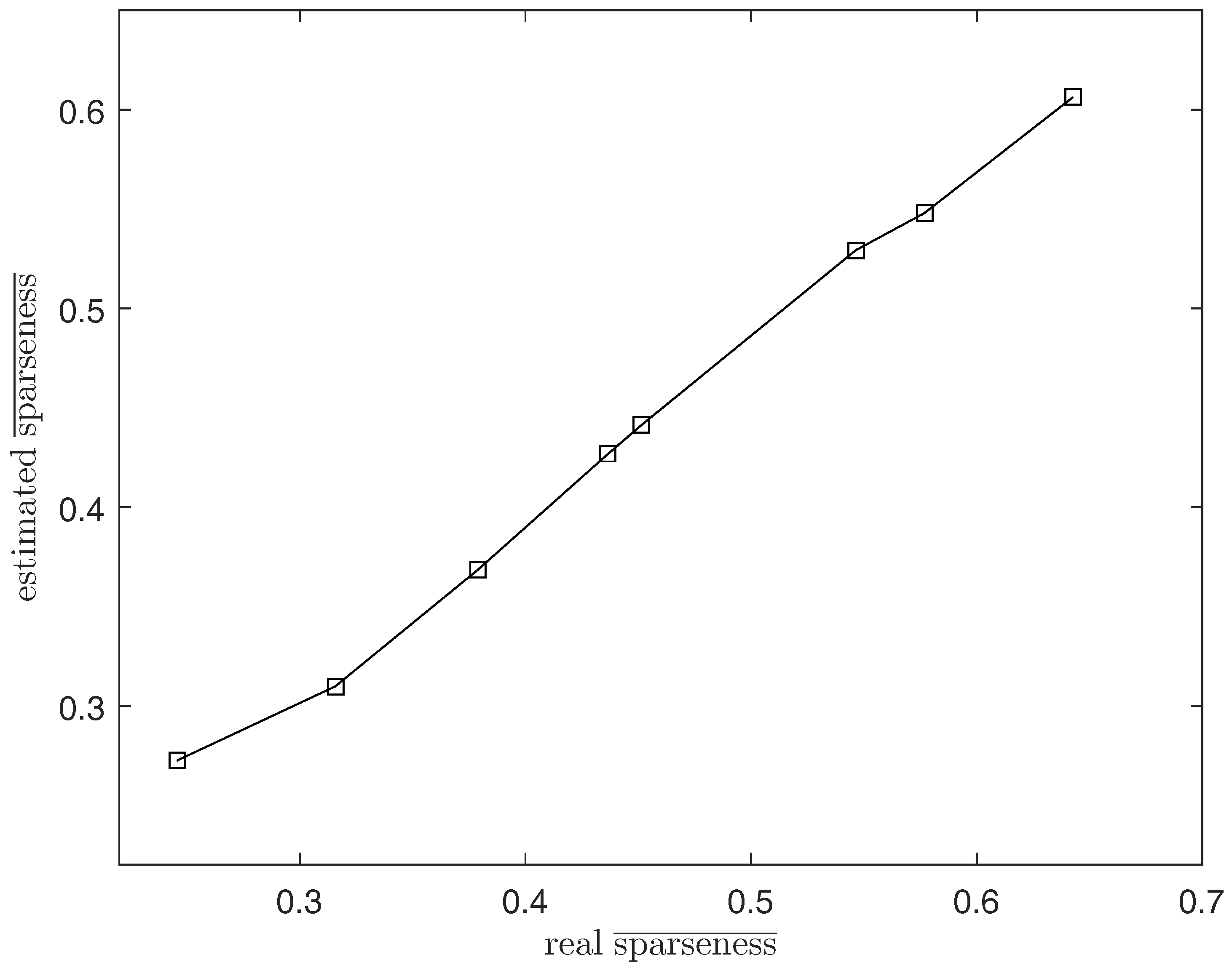
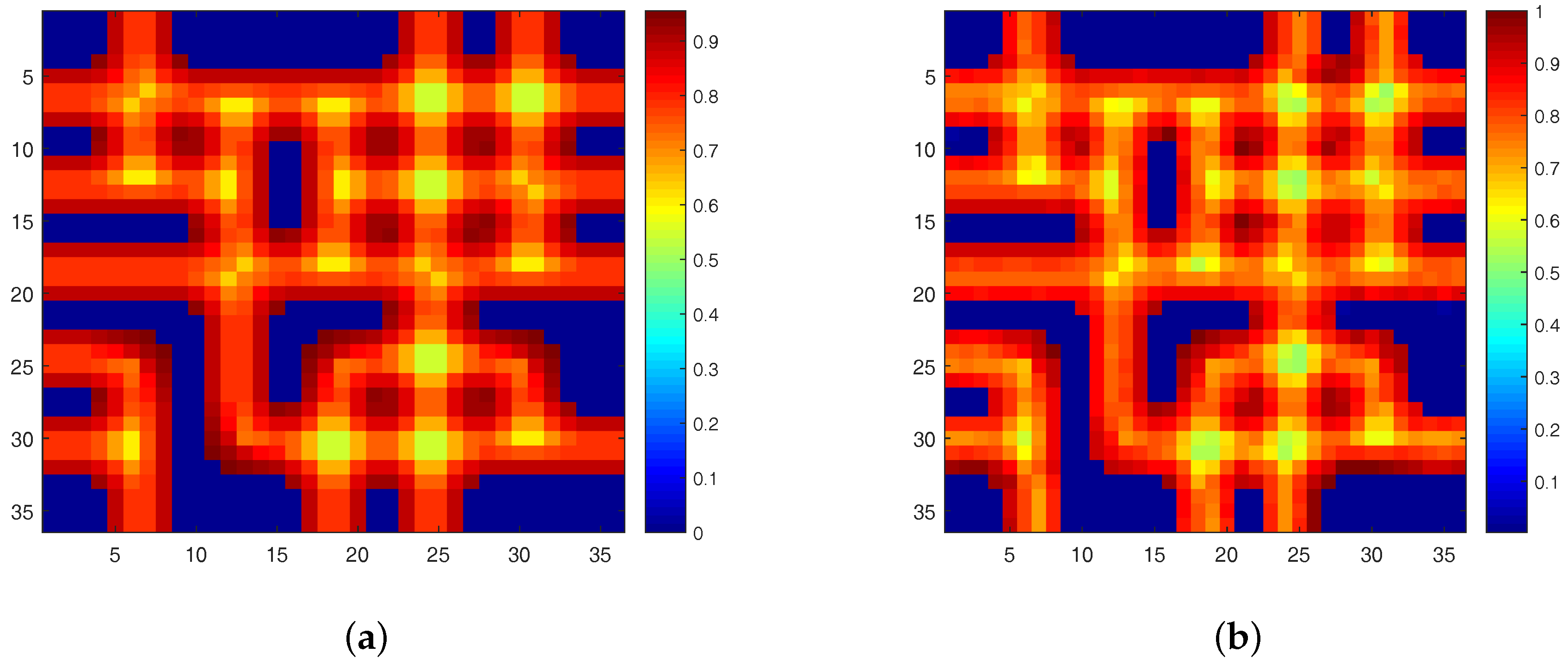
To solve this problem, we propose the DGC-NMF algorithm which is designed to impose constraints precisely according to the data’s sparsity levels in different regions. However, the sparsity levels of abundances are previously unknown since the ground truth of abundance is not available. In the proposed DGC-NMF algorithm, we firstly carry out an unmixing process based on NMF with no constraint to derive the sparseness map of data. No sparseness constraint is employed in this unmixing process to avoid the distinctive sparsity information of a pixel’s abundances being interfered with by a sparseness constraint without verification. This method of estimating sparseness maps may be a biased way. However, it is still a good choice for estimating sparsity levels since the ground truth of real hyperspectral data is not available and a small sparseness error is tolerable in our proposed DGC-NMF algorithm. To demonstrate the accuracy of the sparseness estimation, experiments are conducted to make comparison between estimated and real sparsity levels of data. Figure 2 shows that the estimated sparsity levels fit the real sparsity levels well under various sparsity levels. The estimated sparseness values could correctly reflect the general trend of the real sparsity levels. Figure 3 presents the real and the estimated sparseness map of synthetic data. The estimated map coincides with the real map well. For regions possessing high or low sparsity levels, the estimate sparseness map also shows high or low values. The estimated sparseness values can represent the real sparsity levels of pixels well. We also conduct experiments in Section 4.1 to compare DGC-NMF with the real sparseness map and DGC-NMF with the estimated sparseness map. The results also validate that it is practical to estimate sparsity levels via the unmixing result of NMF algorithm.
3.2. DGC-NMF Algorithm
Using the sparsity information learnt in Section 3.1, the proposed NMF with data-guided constraints decides whether the constraint or the constraint should be assigned to a pixel. In the DGC-NMF algorithm, both the regularizer and the regularizer are adopted to achieve better control of sparsity in each pixel’s abundances. Pixels are split into two categories according to sparsity levels. For pixels with high sparsity levels, the regularizer is adopted to constrain their abundance. For pixels with low sparsity levels, the regularizer is applied. The model of DGC-NMF is as follows:
where and are the regularization parameter, and and are the indictor matrices which decide whether an constraint constraint or an constraint is imposed or not for each pixel. is obtained by evaluating the sparse levels of abundances of all pixels
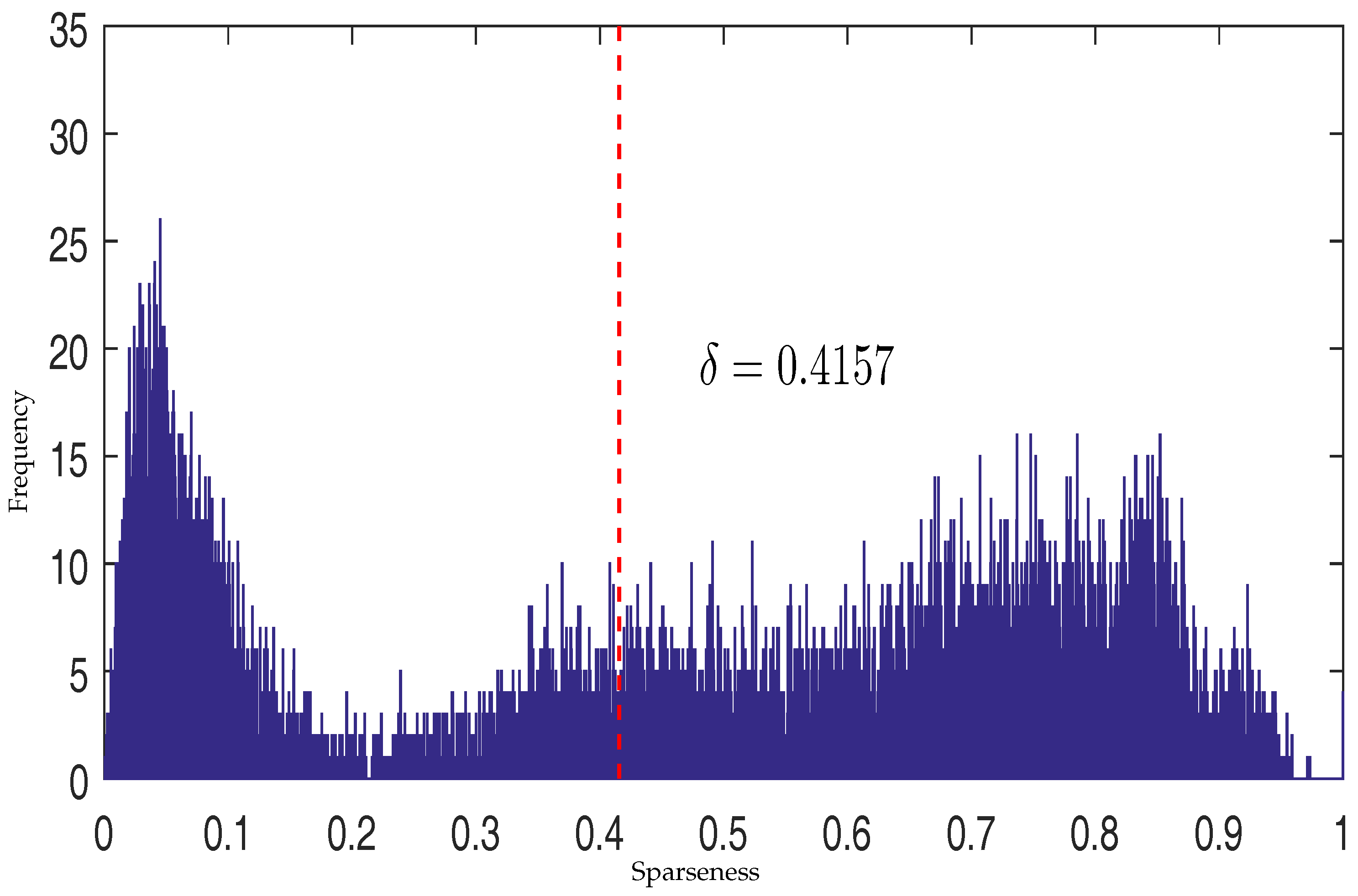
where is a threshold that controls which kind of constraint should be imposed. The threshold is decided by applying Otsu’s method to maximize the separability of pixels with high sparsity level and pixels with low sparsity level [38]. Figure 4 shows the histogram of estimated sparseness values for pixels in a synthetic image and the selected value of threshold for this synthetic image. The sparseness histogram is obtained by counting the sparseness of estimated abundance of pixels. When the sparseness of a pixel’s abundance is higher than , the pixel’s abundance will be constrained by an sparsity regularization. Otherwise, the pixel’s abundance will enjoy an constraint to promote evenness.
The procedure of the proposed DGC-NMF is described in Algorithm 1.
| Algorithm 1 DGC-NMF algorithm |
| Input: Hyperspectral data ; the number of endmembers P. |
Initialization: Initialize endmember matrix and abundance matrix by SGA-FCLS.
|
The update rule for W in Equation (15) is just the same as that in [18]. The authors of [18] have proved objective (2) is nonincreasing under the update rule in Equation (3). Therefore, we only need to focus on proving objective (13) is nonincreasing under the update rule for H in Equation (16).
Since the objective function in Equation (13) is separable by columns, for each column of H, we could consider each column of H individually. For convenience, let h denote a column of H, x denotes the corresponding columns in X, and c, d denote the corresponding column in C, D, respectively. c and d are vectors with all ones or zeros. The objective function by column is expressed as follows:
An auxiliary function similar to that used in the expectation-maximization algorithm is defined to prove Theorem 1 [39,40].
Definition 1.
is an auxiliary function of with
satisfied
Lemma 1.
If is an auxiliary function of , is nonincreasing under the update
Proof.
☐
Obviously, the second property of G defined in Definition 1 is satisfied. Writing out the Taylor expansion of
where the function R denotes the Lagrange remainder term, which can be omitted.
Comparing with in Equation (20), we find the first property is satisfied when
Equivalent to
where is is a diagonal matrix with diagonal
The positive semidefiniteness of has been proved in [18]. Another term in Equation (23) is nonnegative since c and h both are nonnegative. Thus, Equation (22) holds due to the sum of two positive semidefinite matrices is also positive semidefinite.
It remains to select the minimum of G by taking the gradient and equating to zero
Solving h gets
which is the desired columnwise form of update rule in Equation (16). The proof of Theorem 1 is completed.
4. Experimental Results and Analysis
4.1. Experiments on Synthetic Data
In this section, the proposed DGC-NMF algorithm is tested on synthetic data to evaluate its performance. Three related methods, including NMF [20], -NMF [35] and -NMF [41] are used for comparison with the proposed method. The synthetic data used to test is generated following [29]. The spectral signatures are randomly selected from the United States Geological Survey (USGS) digital spectral library to simulate synthetic images [42]. The abundances are generated as follows. Firstly, a size image is divided into regions. Each region is initialized with the same kind of ground material. Secondly, a low-pass filter is applied to generated mixed pixels and make the abundance variation smooth. Finally, a threshold is used to reject pixels with high purity. The pixels with abundance larger than will be replaced by mixtures of all endmembers with equal abundance. can be used as the parameter to generate synthetic data with various sparseness levels. In addition, zero-mean white Gaussian noise is added into the synthetic data to simulate possible noise. In the experiments on synthetic data and real data, DGC-NMF and the compared NMF based algorithms are all initialized using SGA-FCLS. SGA-FCLS provides a more accurate initialization than random initialization. We also compared the unmixing performance of our proposed DGC-NMF with that of SGA-FCLS in Section 4.2.
Two criteria, spectral angle distance (SAD) and root-mean-square error (RMSE), are adopted to evaluate the unmixing performance of algorithms. They are defined as follows:
where and are the reference endmember signatures and their estimates. Respectively, and are the reference and estimated abundances. Before calculating evaluation criteria, the estimated endmembers should firstly be reordered to match the reference endmembers. The estimated abundances should also be reordered respectively.
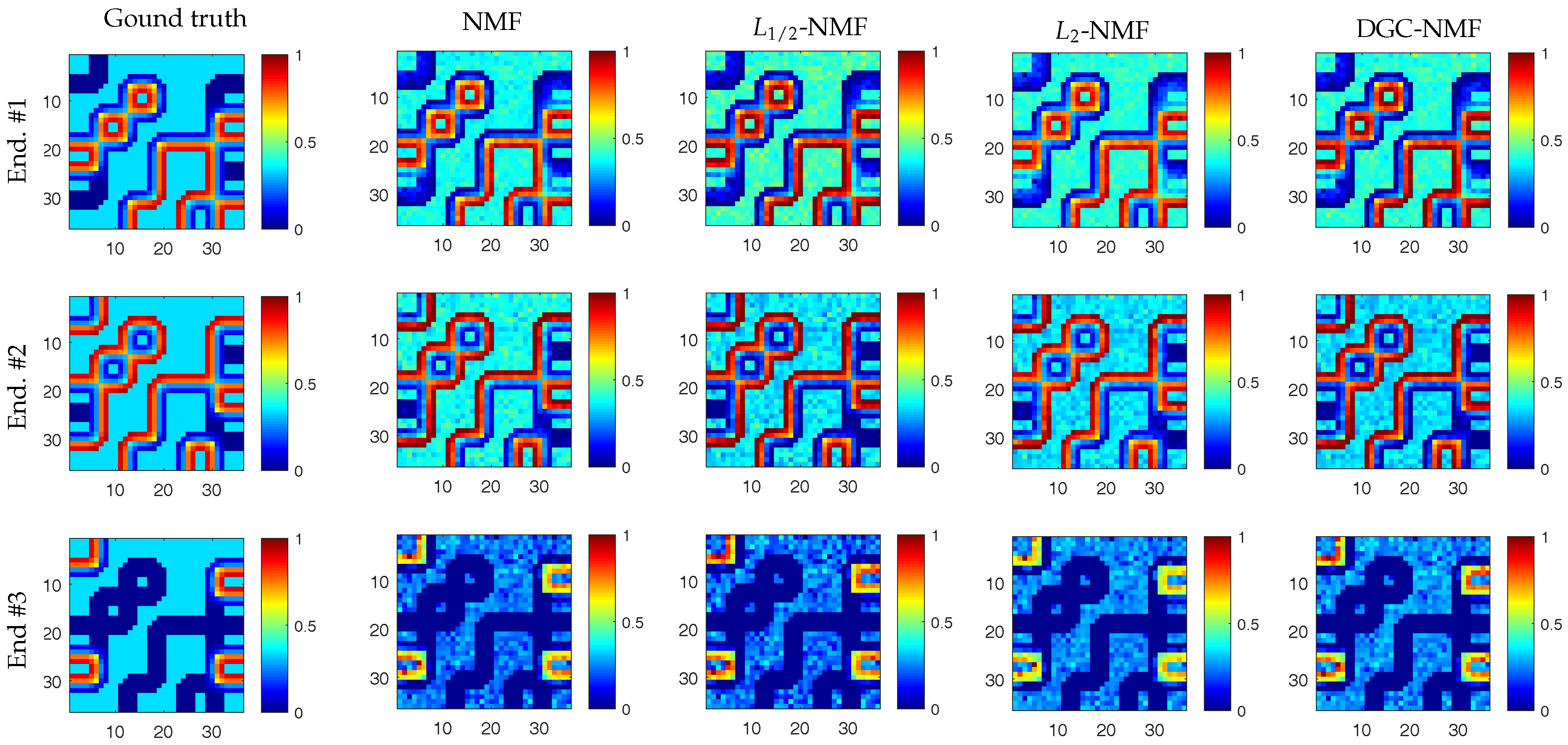
To present the effects of algorithms on the sparseness of unmixing results intuitively, we compare the sparseness histograms of different algorithms in Figure 5. The histogram are obtained by counting the sparseness levels of pixels’ abundance estimated by different algorithms. From the histogram in Figure 5b, it can be seen that the abundance result achieved by -NMF generally tends to be smoother. The histogram of -NMF owns more pixels with low sparseness levels compared to other algorithms. In Figure 5c, the whole histogram of -NMF has the tendency of a right shift, which demonstrates that -NMF can effectively promote sparsity in the unmixing process. The sparseness of pixels’ abundances will be raised when applying -NMF. The pixels with various sparseness are not able to receive constraints accommodated to their sparsity levels in -NMF and -NMF. For the histogram of DGC-NMF in Figure 5d, the right part of the histogram has the tendency towards a right shift and the left part has a tendency towards a left shift. This validates that the DGC-NMF algorithm can impose adaptive constraints on pixels according to their sparseness of abundances. Figure 6 shows the abundance maps of NMF, -NMF, -NMF, and DGC-NMF, respectively, when applied on synthetic data. It can be seen that DGC-NMF achieves sparser abundance results than NMF and -NMF in areas possessing high sparsity levels. Meanwhile, DGC-NMF obtains more accurate abundance results than -NMF in evenly mixed areas.
Due to the first unmixing process for learning sparseness maps from data, the proposed DGC-NMF is more computationally expensive than -NMF and -NMF. However, it is still in the same order of magnitude as -NMF and -NMF. Table 1 shows the running time of different algorithms on a size synthetic image. For each algorithm, 20 independent runs are carried out and the results are averaged. All experiments are performed using a laptop PC with an Intel Core I7 CPU and 8 GB of RAM. The iteration number of the two steps in DGC-NMF is set as 200. The iteration number of comparative algorithms is also set as 200.
To further analyze the performance of algorithms, five experiments are conducted with respect to the following: (1) sparseness; (2) size of image; (3) number of endmembers; and (4) the signal-to-noise ratio (SNR). For each experiment, 20 independent runs are carried out and the results are averaged. Considering DGC-NMF has the same parameters and as -NMF and -NMF, we set and in DGC-NMF to the same values as those of -NMF and -NMF to make fair comparisons. The values of parameters and for -NMF and -NMF, respectively, are carefully determined to achieve best results as in [33]. DGC-NMF adopts the same values of parameters to validate the effectiveness.
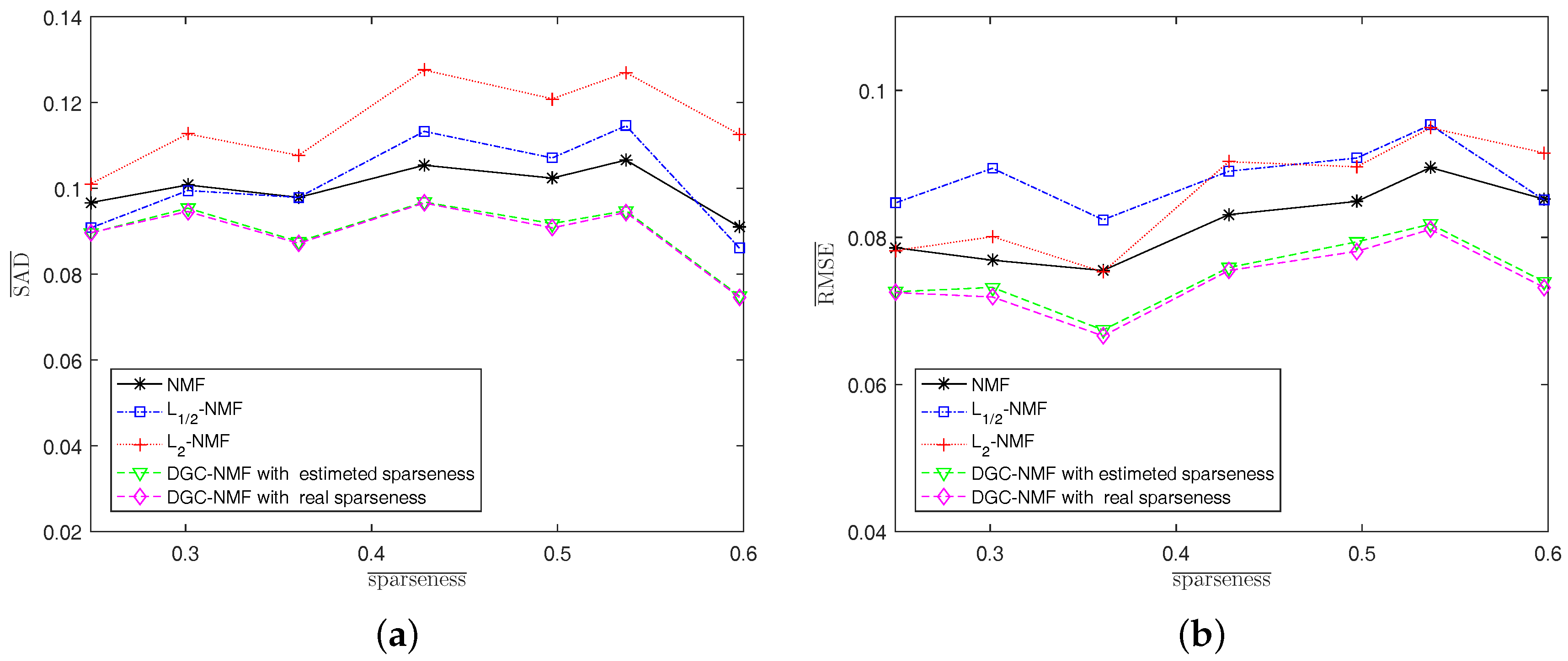
Experiment 1: In this experiment, we investigate the performance of algorithms under various sparsity levels. Since the real abundance maps of synthetic data are available, we also make comparison between DGC-NMF with a real sparseness map and DGC-NMF with an estimated sparseness map. The algorithms are tested on synthetic data with different average sparseness levels of abundances. The size of data used here and in the following experiments is , except in Experiment 2. The endmember number K = 6 and SNR = 20 dB. Figure 7 shows that the proposed DGC-NMF performs the best at various sparseness levels. The DGC-NMF with estimated sparseness map performs quite closely with the DGC-NMF with the real sparseness map, which proves the effectiveness of the proposed method for estimating the sparsity levels of pixels’ abundances. For SAD, DGC-NMF performs the best, while -NMF has the poorest performance. With the sparseness level rises to 0.6, -NMF achieves better performance than -NMF and NMF, while still being inferior to DGC-NMF. Considering RMSE, DGC-NMF also achieves the best performance under different sparseness levels. -NMF achieves more accurate results than -NMF when applied to data with relatively low sparsity levels.
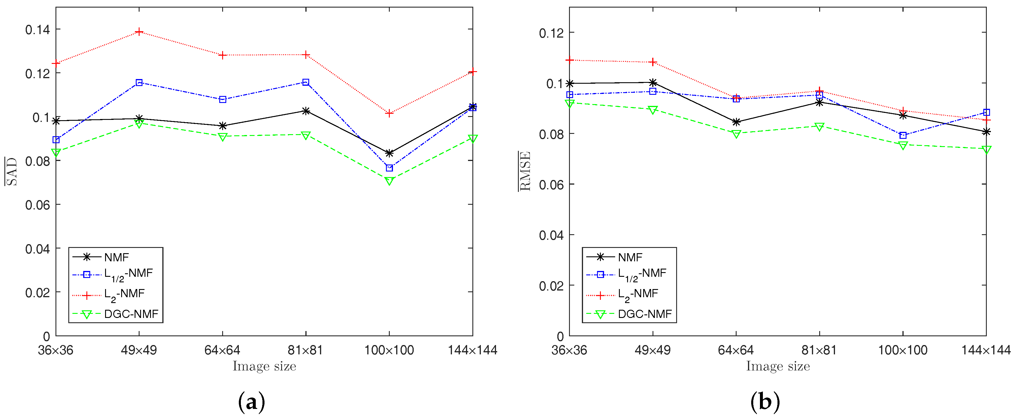
Experiment 2: The algorithms are also tested on synthetic data with different sizes to validate the performance. The image size is set as , respectively, with K = 6, and SNR = 20 dB. In this experiment and following experiments, the threshold is set as 0.91. Figure 8 shows that the proposed DGC-NMF achieves best results for either SAD or RMSE when applied to different sizes of images. For larger images, -NMF and -NMF may not obtain a satisfactory result since the images consist of areas with various sparsity levels and a simple constraint is not applicable. The proposed method provides a reliable way for images possessing areas with various sparsity levels and requiring adaptive constraints.
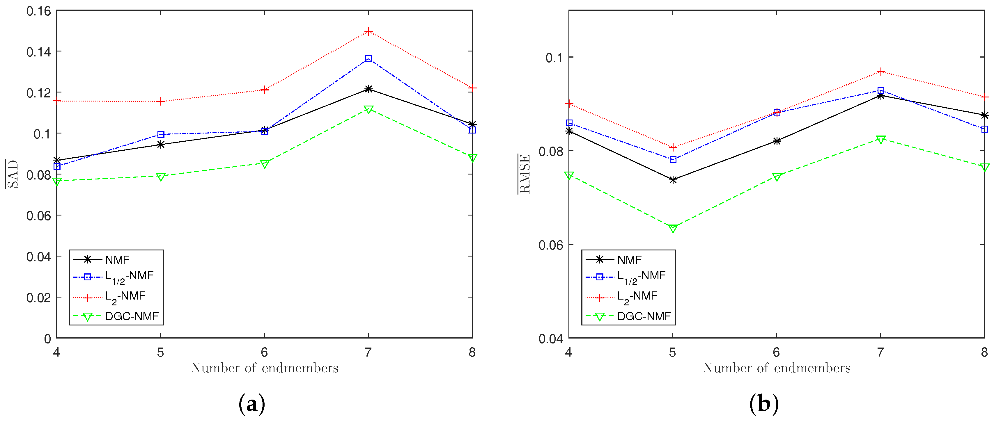
Experiment 3: The algorithms’ performance when the number of endmembers changes is presented in Figure 9a,b. The number of endmembers is set from 4 to 8 and the SNR is also set as 20 dB. Generally, DGC-NMF performs the best while -NMF performs the worst when the number of endmembers varies. For SAD, DGC-NMF still gains the best results, while -NMF performs the worst and -NMF and NMF have similar performance. From Figure 9b, we can see that DGC-NMF also achieves the lowest RMSE values when applied to data with different number of endmembers.
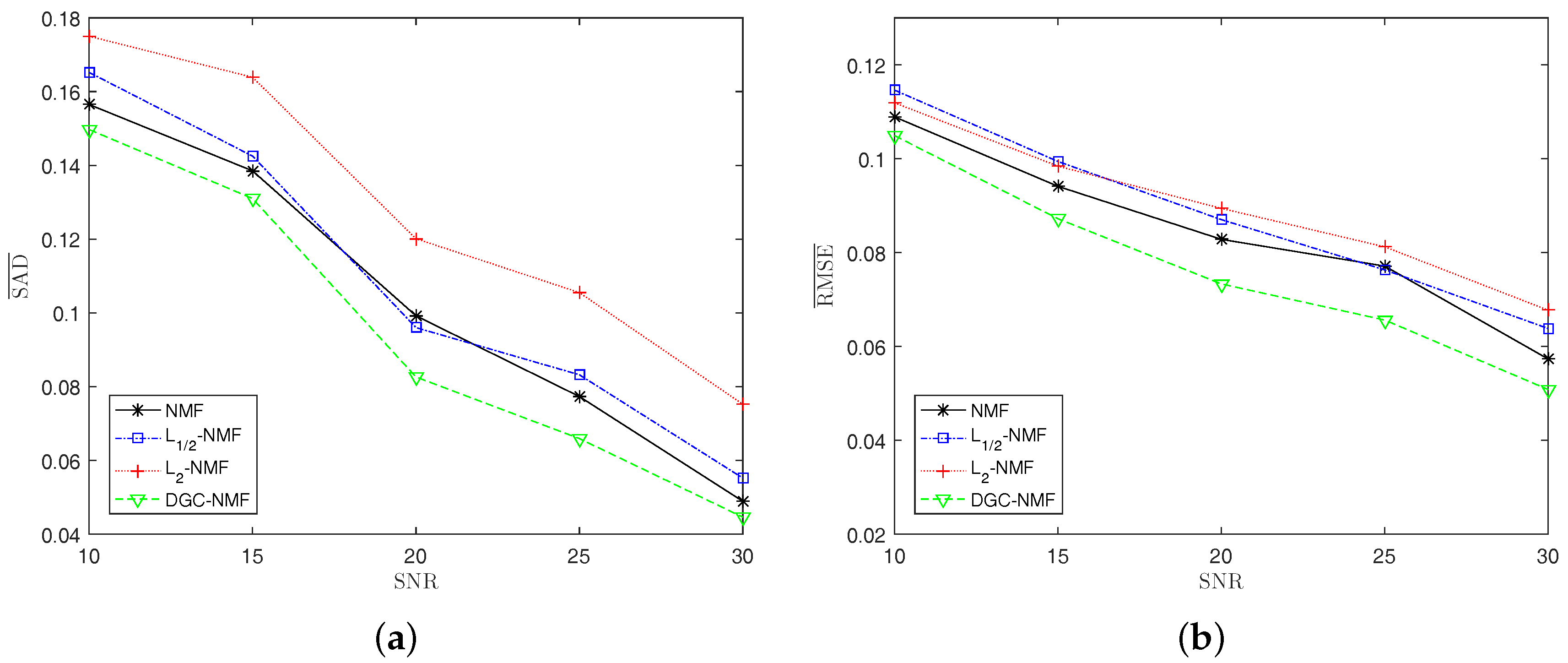
Experiment 4: To test the robustness of the proposed method, synthetic data with different noise levels are used to examine the performance of algorithms. We change the SNR of synthetic data from 10 dB to 30 dB at the steps of 5 dB. With the increase of noise level, the performance of algorithms degrades as expected. The DGC-NMF shows the best performance as the SNR varies. For SAD, -NMF yields better results than -NMF and NMF when SNR = 20. For RMSE, NMF is better than -NMF and -NMF. It can be seen from the Figure 10 that the proposed DGC-NMF is not sensitive to noise compared to other three algorithms.
4.2. Experiments on Real Data
In this section, we present the experimental results of the proposed method on real hyperspectral data. Two hyperspectral datasets which include regions with different sparsity levels in an urban scene and a regional mineral scene are used in the experiments. To verify the performance of the proposed method, the results of DGC-NMF are compared with NMF [20], -NMF [35], and -NMF [41]. VCA-FCLS and SGA-FCLS are also adopted to compare with the proposed method. The dimensionality reduction (DR) method adopted for SGA here is principal component analysis (PCA) [43]. The initial condition for SGA in this paper is set as starting with two endmembers with maximal segment produced by the one-dimensional two-vertex simplex with maximal distance. The experiment for VCA-FCLS is repeated 10 times. The results are averaged values and the standard deviations are taken. Since the result of SGA is consistent, there is no standard deviation reported for SGA-FCLS and NMF-based methods. The standard deviation of VCA-FCLS comes from the randomness of VCA.
The first hyperspectral scene to be used is the urban dataset collected by a Hyperspectral Digital Imagery Collection Experiment (HYDICE) sensor over an area located at Copperas Cove near Fort Hood, TX, U.S., in October 1995. The spectral and spatial resolutions are 10 nm and 2 m, respectively. After the bands with low SNR are removed from the original dataset, only 162 bands remain in the experiment (i.e., L = 162). The image is pixels in size and consists of a suburban residential area as shown in Figure 11a. There are four targets of interest existing in this area: asphalt, grass, roofs, and trees. Since the ground truth of Urban dataset is not available. We use the reference abundance maps obtained from [44] to evaluate the algorithms’ performance. Two criteria, spectral angle distance (SAD) and root-mean-square error (RMSE), are adopted to evaluate the accuracy of estimated endmembers and abundances, respectively.
Table 2 represents the mean values and standard deviations of SAD of different methods on urban data. The rows respectively show the results of four targets of interest, i.e., ‘asphalt’, ‘grass’, ‘trees’ and ‘roofs’, along with the mean values. From the Table 2, it can be seen that the SAD results achieved by DGC-NMF are better than those of other methods in general. For target ’roofs’ and the mean value, the proposed DGC-NMF achieves the best results. For ‘asphalt’ and ‘trees’, DGC-NMF achieves the second best result. The RMSE results of algorithms are illustrated in Table 3. We can also find that the DGC-NMF’s results are generally better than those yielded by the other algorithms. For ‘asphalt’, ‘grass’ and the mean value, DGC-NMF achieves the best results. For ‘trees’ and ‘roofs’, DGC-NMF achieves the second best results.
In Figure 12, the endmember signatures obtained by different methods are displayed with reference to the ground truth for visual comparison. It is shown that the endmember signatures obtained by DGC-NMF are in good accordance with the ground truth. Figure 13 shows the sparseness maps of abundance results obtained by -NMF, -NMF, and DGC-NMF, respectively. It can be seen that the sparseness values in the map of -NMF are low as a whole, while those of -NMF show relatively high levels. For the proposed DGC-NMF, the sparseness values are in better accordance with the distribution of ground covers in hyperspectral data. In high sparsity level areas such as the areas composed of asphalt, DGC-NMF acts in a similar manner to -NMF. In these areas, DGC-NMF promotes constraint and obtains sparser abundance results. In areas with low sparsity levels that are evenly mixed with signatures such as the areas with both trees and grass, DGC-NMF promotes constraint adaptively and obtains smoother abundance results of pixels. Therefore, the sparseness values are lower than those of -NMF, similar to -NMF. Figure 14 shows the separated abundance maps of each endmember by VCA-FCLS, SGA-FCLS, NMF, -NMF, -NMF, and DGC-NMF, respectively. As shown in the figure, all algorithms separate out the four targets successfully. Through visual comparison, we can see that -NMF and -NMF obtain smoother and sparser results than NMF, respectively. -NMF achieves great results in high sparsity level areas, but fails to capture mixed information in evenly mixed areas. The proposed DGC-NMF achieves sparser abundance maps than -NMF, and has better abundance estimation than -NMF in transition regions. Generally, Figure 13 and Figure 14 demonstrate that the proposed DGC-NMF could promote adaptive constraints on areas in hyperspectral images with various sparsity levels and achieve better unmixing results of abundance.
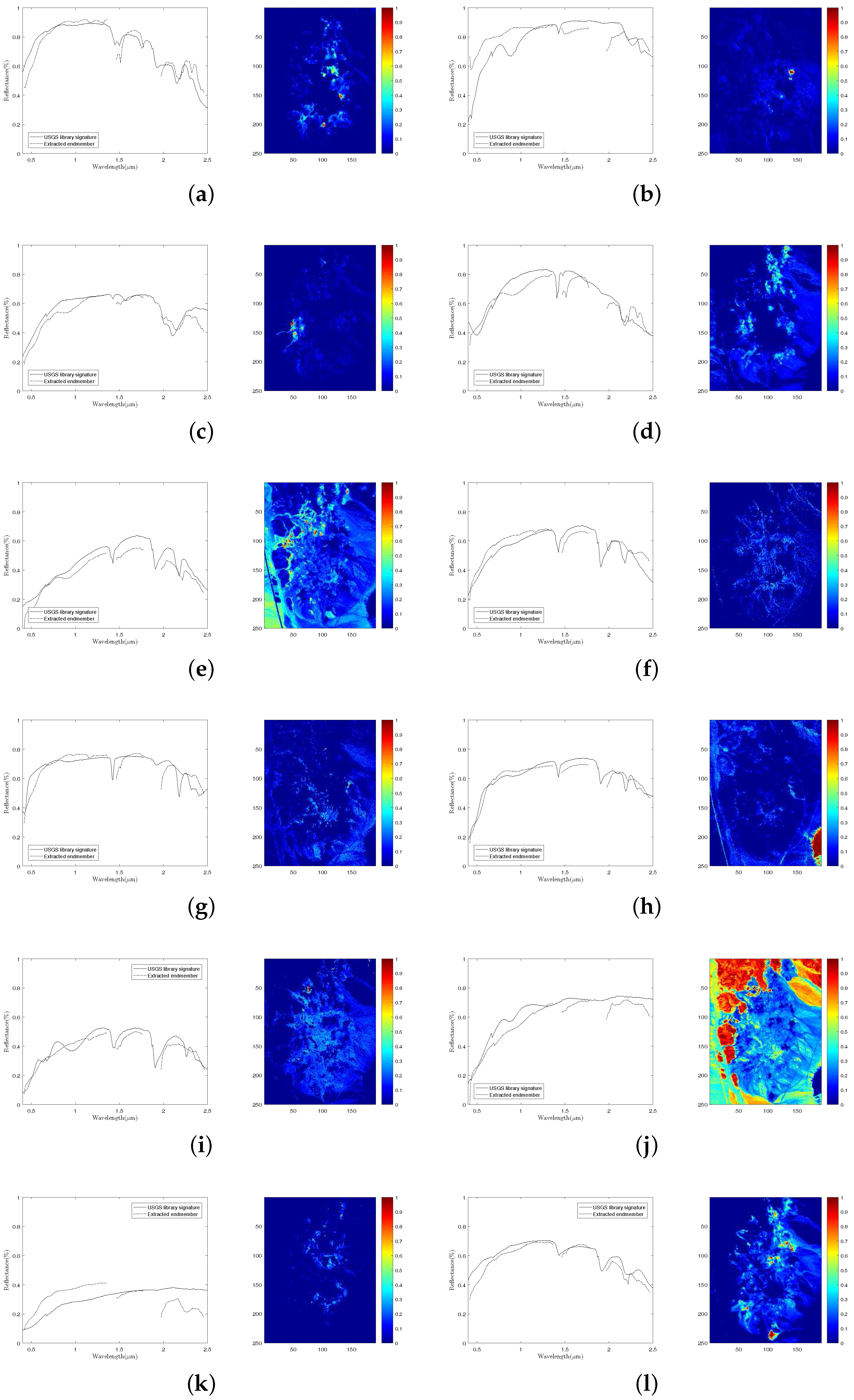
To validate the performance of our proposed method on hyperspectral data with various sparsity levels, we also conduct an experiment on the Cuprite data. The well known Cuprite dataset is collected by an airborne visible/infrared imaging spectrometer (AVIRIS) sensor over Cuprite mining site, Nevada. The raw images have 224 spectral bands covering the wavelength ranging from 0.4 µm to 2.5 µm. The spatial resolution is 20 m and the spectral resolution is 10 nm. Approximate distributions of the minerals have been illustrated in many pieces of research [10,22,26]. The image used in our experiment is a pixel subset of the Cuprite scene, as shown in Figure 11b. Due to the water absorption and low SNR, several bands are removed, including bands 1–2, 104–113, 148–167, and 221–224. Hence, 188 bands are used in the experiment. According to [10], there are 14 kinds of minerals existing in the scene. However, the variants of the same mineral have minor differences between each other and could be considered as the same endmember. Therefore, we set the number of endmembers in the scene to 12 [25,33]. Figure 15 presents the extracted endmembers and their corresponding abundance maps by DGC-NMF. In the figure, the extracted signatures are compared with USGS library spectra and show good accordance with them. Table 4 presents the SAD results of the proposed DGC-NMF, along with those of other methods. It shows that DGC-NMF achieves the greatest number of cases of best SAD results, outperforming NMF, -NMF, and -NMF. -NMF obtains the most second-best SAD results of endmembers. In the terms of mean value, DGC-NMF performs the best.
5. Conclusions
In this paper, we provide a novel nonnegative matrix factorization with data-guided constraint (DGC-NMF), which is based on the data’s sparsity levels in different areas. Since the sparseness of abundances is previously unknown, we provide a method to evaluate the sparsity level of each pixel’s abundances. The sparseness map of data is estimated by using the obtained abundances in a NMF unmixing process with no constraint. The experiments results validate that the estimated sparseness values can represent the real sparsity levels of pixels well. Through the estimated sparseness map, sparseness constraints on pixels’ abundances could be adaptively imposed and lead to better unmixing results. We have proven monotone decrease of the objective by our algorithm and illustrated the effectiveness and practicability of the algorithm by experiments on synthetic data and real hyperspectral images. For the future work, the performance of our method could be further improved by achieving a more accurate estimation of sparsity levels and by introducing more reasonable constraints imposing strategy. More methods based on mining and using the information latent in data itself would also be worthy of further study.
Acknowledgments
This work was supported by National Nature Science Foundation of China (No. 61571170, No. 61671408 ) and the Joint Funds of the Ministry of Education of China (No. 6141A02022314).
Author Contributions
All the authors made significant contributions to the work. Risheng Huang designed the research and analyzed the results. Xiaorun Li provided advice for the preparation and revision of the paper. Liaoying Zhao assisted in the preparation work and validation work.
Conflicts of Interest
The authors declare no conflict of interest.
References
- Bioucas-Dias, J.M.; Plaza, A.; Dobigeon, N.; Parente, M.; Du, Q.; Gader, P.; Chanussot, J. Hyperspectral unmixing overview: Geometrical, statistical, and sparse regression-based approaches. IEEE J. Sel. Top. Appl. Earth Obs. Remote Sens. 2012, 5, 354–379. [Google Scholar] [CrossRef]
- Altmann, Y.; Dobigeon, N.; Tourneret, J.Y. Unsupervised post-nonlinear unmixing of hyperspectral images using a Hamiltonian Monte Carlo algorithm. IEEE Trans. Image Process. 2014, 23, 2663–2675. [Google Scholar] [CrossRef] [PubMed] [Green Version]
- Wang, Y.; Pan, C.; Xiang, S.; Zhu, F. Robust hyperspectral unmixing with correntropy-based metric. IEEE Trans. Image Process. 2015, 24, 4027–4040. [Google Scholar] [CrossRef] [PubMed]
- Wei, Q.; Chen, M.; Tourneret, J.Y.; Godsill, S. Unsupervised nonlinear spectral unmixing based on a multilinear mixing model. IEEE Trans. Geosci. Remote Sens. 2017, 55, 4534–4544. [Google Scholar] [CrossRef]
- Qian, Y.; Xiong, F.; Zeng, S.; Zhou, J.; Tang, Y.Y. Matrix-vector nonnegative tensor factorization for blind unmixing of hyperspectral imagery. IEEE Trans. Geosci. Remote Sens. 2017, 55, 1776–1792. [Google Scholar] [CrossRef]
- Dobigeon, N.; Tourneret, J.Y.; Chang, C.I. Semi-supervised linear spectral unmixing using a hierarchical Bayesian model for hyperspectral imagery. IEEE Trans. Signal Process. 2008, 56, 2684–2695. [Google Scholar] [CrossRef] [Green Version]
- Altmann, Y.; Halimi, A.; Dobigeon, N.; Tourneret, J.Y. Supervised nonlinear spectral unmixing using a postnonlinear mixing model for hyperspectral imagery. IEEE Trans. Image Process. 2012, 21, 3017–3025. [Google Scholar] [CrossRef] [PubMed] [Green Version]
- Boardman, J.W. Geometric mixture analysis of imaging spectrometry data. In Proceedings of the 14th Annual International Geoscience and Remote Sensing Symposium: Surface and Atmospheric Remote Sensing: Technologies, Data Analysis and Interpretation, Pasadena, CA, USA, 8–12 August 1994; Volume 4, pp. 2369–2371. [Google Scholar]
- Winter, M.E. N-FINDR: An algorithm for fast autonomous spectral end-member determination in hyperspectral data. In Proceedings of the SPIE’s International Symposium on Optical Science, Engineering, and Instrumentation, Denver, CO, USA, 18–23 July 1999; pp. 266–275. [Google Scholar]
- Nascimento, J.M.; Dias, J.M. Vertex component analysis: A fast algorithm to unmix hyperspectral data. IEEE Trans. Geosci. Remote Sens. 2005, 43, 898–910. [Google Scholar] [CrossRef]
- Chang, C.I.; Wu, C.C.; Liu, W.; Ouyang, Y.C. A new growing method for simplex-based endmember extraction algorithm. IEEE Trans. Geosci. Remote Sens. 2006, 44, 2804–2819. [Google Scholar] [CrossRef]
- Chang, C.I.; Wen, C.H.; Wu, C.C. Relationship exploration among PPI, ATGP and VCA via theoretical analysis. Int. J. Comput. Sci. Eng. 2013, 8, 361–367. [Google Scholar] [CrossRef]
- Li, H.; Chang, C.I. Linear spectral unmixing using least squares error, orthogonal projection and simplex volume for hyperspectral Images. In Proceedings of the 7th Workshop Hyperspectral Image & Signal Processing: Evolution Remote Sensing (WHISPERS), Tokyo, Japan, 2–5 June 2015; pp. 2–5. [Google Scholar]
- Chang, C.I.; Chen, S.Y.; Li, H.C.; Chen, H.M.; Wen, C.H. Comparative study and analysis among ATGP, VCA, and SGA for finding endmembers in hyperspectral imagery. IEEE J. Sel. Top. Appl. Earth Obs. Remote Sens. 2016, 9, 4280–4306. [Google Scholar] [CrossRef]
- Dobigeon, N.; Tourneret, J.Y. Spectral unmixing of hyperspectral images using a hierarchical Bayesian model. In Proceedings of the IEEE International Conference on Acoustics, Speech and Signal Processing, Honolulu, HI, USA, 16–20 April 2007; Volume 3. [Google Scholar]
- Dobigeon, N.; Moussaoui, S.; Coulon, M.; Tourneret, J.Y.; Hero, A.O. Joint Bayesian endmember extraction and linear unmixing for hyperspectral imagery. IEEE Trans. Signal Process. 2009, 57, 4355–4368. [Google Scholar] [CrossRef] [Green Version]
- Themelis, K.E.; Rontogiannis, A.A.; Koutroumbas, K.D. A novel hierarchical Bayesian approach for sparse semisupervised hyperspectral unmixing. IEEE Trans. Signal Process. 2012, 60, 585–599. [Google Scholar] [CrossRef]
- Lee, D.D.; Seung, H.S. Algorithms for non-negative matrix factorization. In Advances in Neural Information Processing Systems; MIT Press: Cambridge, MA, USA, 2001; pp. 556–562. [Google Scholar]
- Zhu, F.; Wang, Y.; Xiang, S.; Fan, B.; Pan, C. Structured sparse method for hyperspectral unmixing. ISPRS J. Photogramm. Remote Sens. 2014, 88, 101–118. [Google Scholar] [CrossRef]
- Lee, D.D.; Seung, H.S. Learning the parts of objects by non-negative matrix factorization. Nature 1999, 401, 788–791. [Google Scholar] [PubMed]
- Wang, N.; Du, B.; Zhang, L. An endmember dissimilarity constrained non-negative matrix factorization method for hyperspectral unmixing. IEEE J. Sel. Top. Appl. Earth Obs. Remote Sens. 2013, 6, 554–569. [Google Scholar] [CrossRef]
- Miao, L.; Qi, H. Endmember extraction from highly mixed data using minimum volume constrained nonnegative matrix factorization. IEEE Trans. Geosci. Remote Sens. 2007, 45, 765–777. [Google Scholar] [CrossRef]
- Huck, A.; Guillaume, M. Robust hyperspectral data unmixing with spatial and spectral regularized NMF. In Proceedings of the 2nd Workshop on Hyperspectral Image and Signal Processing: Evolution in Remote Sensing (WHISPERS), Reykjavik, Iceland, 14–16 June 2010; pp. 1–4. [Google Scholar]
- Tong, L.; Zhou, J.; Qian, Y.; Bai, X.; Gao, Y. Nonnegative-matrix-factorization-based hyperspectral unmixing with partially known endmembers. IEEE Trans. Geosci. Remote Sens. 2016, 54, 6531–6544. [Google Scholar] [CrossRef]
- Lu, X.; Wu, H.; Yuan, Y.; Yan, P.; Li, X. Manifold regularized sparse NMF for hyperspectral unmixing. IEEE Trans. Geosci. Remote Sens. 2013, 51, 2815–2826. [Google Scholar] [CrossRef]
- Liu, X.; Xia, W.; Wang, B.; Zhang, L. An approach based on constrained nonnegative matrix factorization to unmix hyperspectral data. IEEE Trans. Geosci. Remote Sens. 2011, 49, 757–772. [Google Scholar] [CrossRef]
- Yuan, Y.; Fu, M.; Lu, X. Substance dependence constrained sparse NMF for hyperspectral unmixing. IEEE Trans. Geosci. Remote Sens. 2015, 53, 2975–2986. [Google Scholar] [CrossRef]
- Xu, Z.; Zhang, H.; Wang, Y.; Chang, X.; Liang, Y. L1/2 regularization. Sci. China Inf. Sci. 2010, 53, 1159–1169. [Google Scholar] [CrossRef]
- Qian, Y.; Jia, S.; Zhou, J.; Robles-Kelly, A. L1/2 Sparsity constrained nonnegative matrix factorization for hyperspectral unmixing. In Proceedings of the International Conference on Digital Image Computing: Techniques and Applications (DICTA), Sydney, Australia, 1–3 December 2010; pp. 447–453. [Google Scholar]
- Pauca, V.P.; Piper, J.; Plemmons, R.J. Nonnegative matrix factorization for spectral data analysis. Linear Algebra Appl. 2006, 416, 29–47. [Google Scholar] [CrossRef]
- Jia, S.; Qian, Y. Constrained nonnegative matrix factorization for hyperspectral unmixing. IEEE Trans. Geosci. Remote Sens. 2009, 47, 161–173. [Google Scholar] [CrossRef]
- Wu, C.; Shen, C. Spectral unmixing using sparse and smooth nonnegative matrix factorization. In Proceedings of the International Conference on Geoinformatics, Kaifeng, China, 20–22 June 2013; pp. 1–5. [Google Scholar]
- Zhu, F.; Wang, Y.; Fan, B.; Xiang, S.; Meng, G.; Pan, C. Spectral unmixing via data-guided sparsity. IEEE Trans. Image Process. 2014, 23, 5412–5427. [Google Scholar] [CrossRef] [PubMed]
- Zhu, F.; Wang, Y.; Fan, B.; Meng, G.; Pan, C. Effective spectral unmixing via robust representation and learning-based sparsity. arXiv, 2014; arXiv:1409.0685. [Google Scholar]
- Qian, Y.; Jia, S.; Zhou, J.; Robles-Kelly, A. Hyperspectral unmixing via L1/2 sparsity-constrained nonnegative matrix factorization. IEEE Trans. Geosci. Remote Sens. 2011, 49, 4282–4297. [Google Scholar] [CrossRef]
- Fan, J.; Li, R. Variable selection via nonconcave penalized likelihood and its oracle properties. J. Am. Stat. Assoc. 2001, 96, 1348–1360. [Google Scholar] [CrossRef]
- Hoyer, P.O. Non-negative matrix factorization with sparseness constraints. J. Mach. Learn. Res. 2004, 5, 1457–1469. [Google Scholar]
- Otsu, N. A threshold selection method from gray-level histograms. IEEE Trans. Syst. Man Cybern. 1979, 9, 62–66. [Google Scholar] [CrossRef]
- Dempster, A.P.; Laird, N.M.; Rubin, D.B. Maximum likelihood from incomplete data via the EM algorithm. J. R. Stat. Soc. Ser. B (Methodol.) 1977, 1–38. [Google Scholar]
- Saul, L.; Pereira, F. Aggregate and mixed-order Markov models for statistical language processing. arXiv, 1997; arXiv:cmp-lg/9706007. [Google Scholar]
- Berry, M.W.; Browne, M.; Langville, A.N.; Pauca, V.P.; Plemmons, R.J. Algorithms and applications for approximate nonnegative matrix factorization. Comput. Stat. Data Anal. 2007, 52, 155–173. [Google Scholar] [CrossRef]
- Clark, R.N.; Swayze, G.A.; Gallagher, A.J.; King, T.V.; Calvin, W.M. The US Geological Survey, Digital Spectral Library, Version 1 (0.2 to 3.0 um); Technical report; Geological Survey (US): Reston, VA, USA, 1993.
- Dunteman, G.H. Principal Components Analysis; Sage Publications, Inc.: Thousand Oaks, CA, USA, 1989. [Google Scholar]
- Zhu, F. Hyperspectral Unmixing Datasets & Ground Truths. Available online: http://www.escience.cn/people/feiyunZHU/Dataset_GT.html (accessed on 5 June 2017).
Figure 1.
(a) Airborne visible/infrared imaging spectrometer (AVIRIS) hyperspectral data of the Cuprite mining district in Nevada, USA; (b) Estimated sparseness map from the obtained abundance.
Figure 1.
(a) Airborne visible/infrared imaging spectrometer (AVIRIS) hyperspectral data of the Cuprite mining district in Nevada, USA; (b) Estimated sparseness map from the obtained abundance.
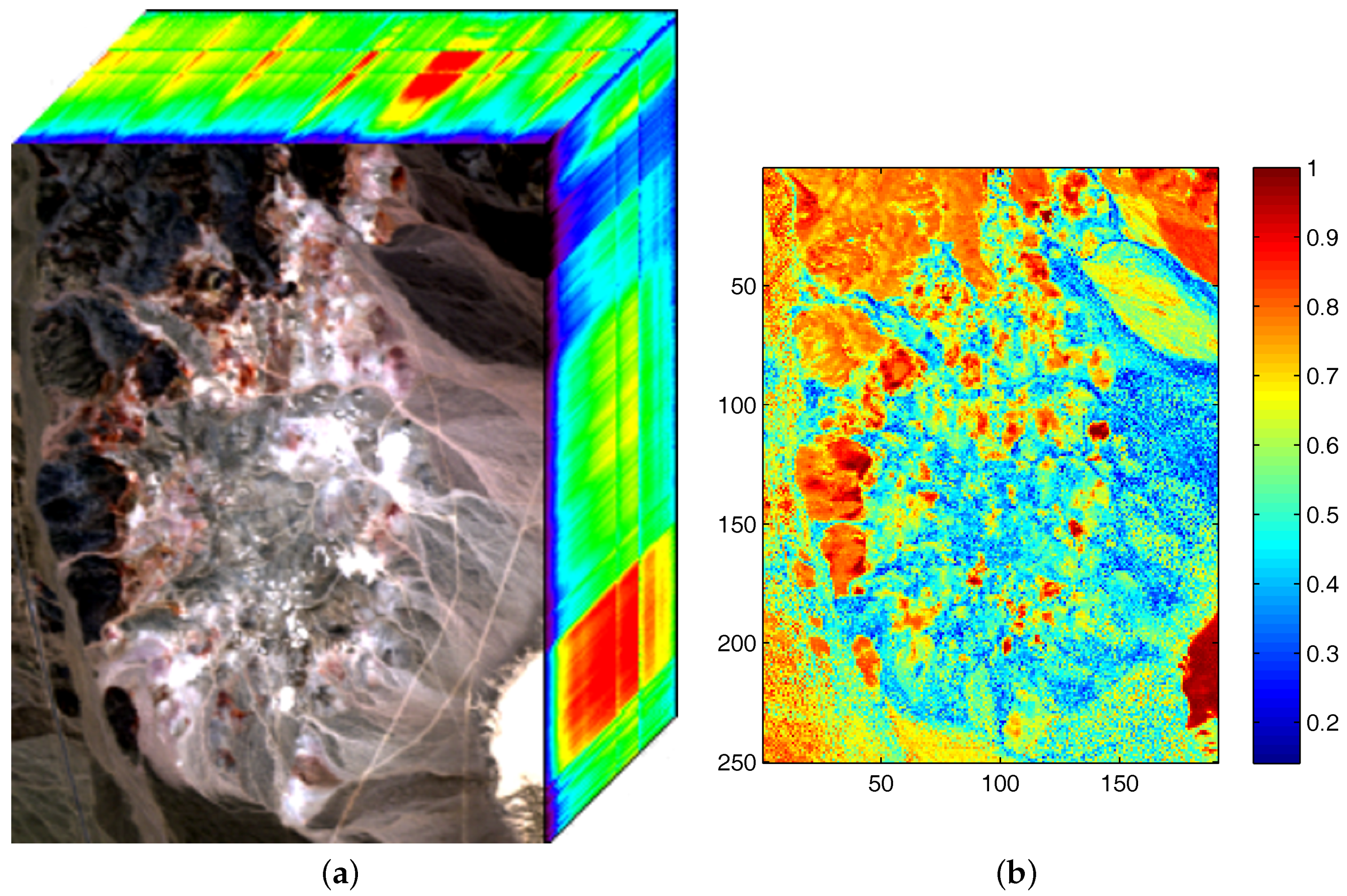
Figure 2.
The real average sparsity level and the estimated average sparsity level.

Figure 3.
(a) The real sparseness map of synthetic data; (b) The estimated sparseness map of synthetic data.
Figure 3.
(a) The real sparseness map of synthetic data; (b) The estimated sparseness map of synthetic data.

Figure 4.
The histogram of estimated sparseness values for pixels in a synthetic image and the selected threshold value.
Figure 4.
The histogram of estimated sparseness values for pixels in a synthetic image and the selected threshold value.

Figure 5.
Comparison of sparseness histograms for true abundances different algorithms’ estimated abundance. (a) Ground truth; (b) -NMF; (c) -NMF; (d) DGC-NMF. NMF: nonnegative matrix factorization; DGC-NMF: NMF with data-guided constraints.
Figure 5.
Comparison of sparseness histograms for true abundances different algorithms’ estimated abundance. (a) Ground truth; (b) -NMF; (c) -NMF; (d) DGC-NMF. NMF: nonnegative matrix factorization; DGC-NMF: NMF with data-guided constraints.
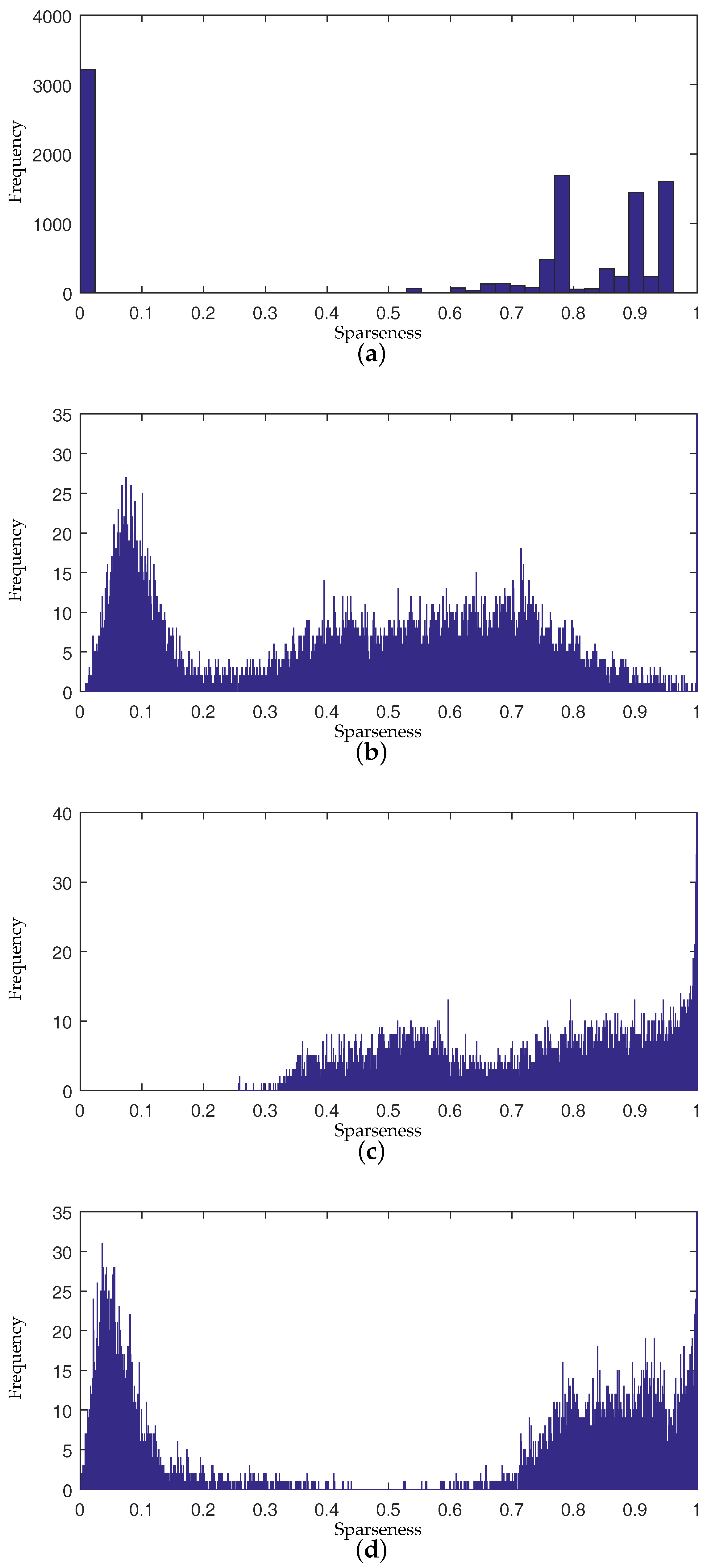
Figure 6.
Abundance maps of synthetic data estimated by NMF, -NMF, -NMF, and DGC-NMF, respectively. Each row shows the corresponding abundance maps of a same endmember by different algorithms.
Figure 6.
Abundance maps of synthetic data estimated by NMF, -NMF, -NMF, and DGC-NMF, respectively. Each row shows the corresponding abundance maps of a same endmember by different algorithms.

Figure 7.
Performance comparison of the algorithms when sparseness level of abundance varies. (a) spectral angle distance (SAD); (b) root-mean-square error (RMSE).
Figure 7.
Performance comparison of the algorithms when sparseness level of abundance varies. (a) spectral angle distance (SAD); (b) root-mean-square error (RMSE).

Figure 8.
Performance comparison of the algorithms with respect to the different sizes of images. (a) SAD; (b) RMSE.
Figure 8.
Performance comparison of the algorithms with respect to the different sizes of images. (a) SAD; (b) RMSE.

Figure 9.
Performance comparison of the algorithms when the number of endmembers varies. (a) SAD; (b) RMSE.
Figure 9.
Performance comparison of the algorithms when the number of endmembers varies. (a) SAD; (b) RMSE.

Figure 10.
Performance comparison of the algorithms under various noise levels. (a) SAD; (b) RMSE.

Figure 11.
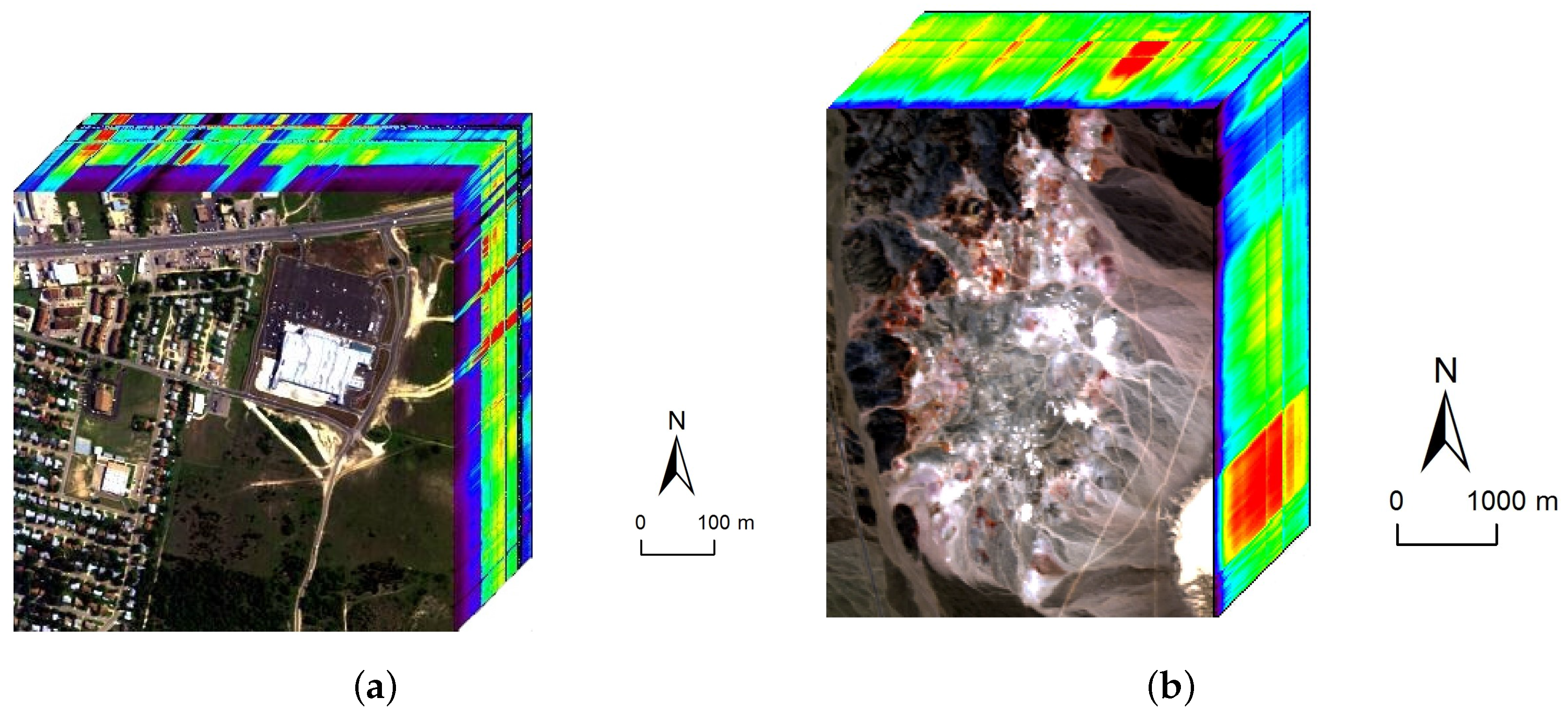
The two real hyperspectral data used in the experiments. (a) The Hyperspectral Digital Imagery Collection Experiment (HYDICE) urban dataset; (b) The airborne visible/infrared imaging spectrometer (AVIRIS) Cuprite dataset.
Figure 11.
The two real hyperspectral data used in the experiments. (a) The Hyperspectral Digital Imagery Collection Experiment (HYDICE) urban dataset; (b) The airborne visible/infrared imaging spectrometer (AVIRIS) Cuprite dataset.

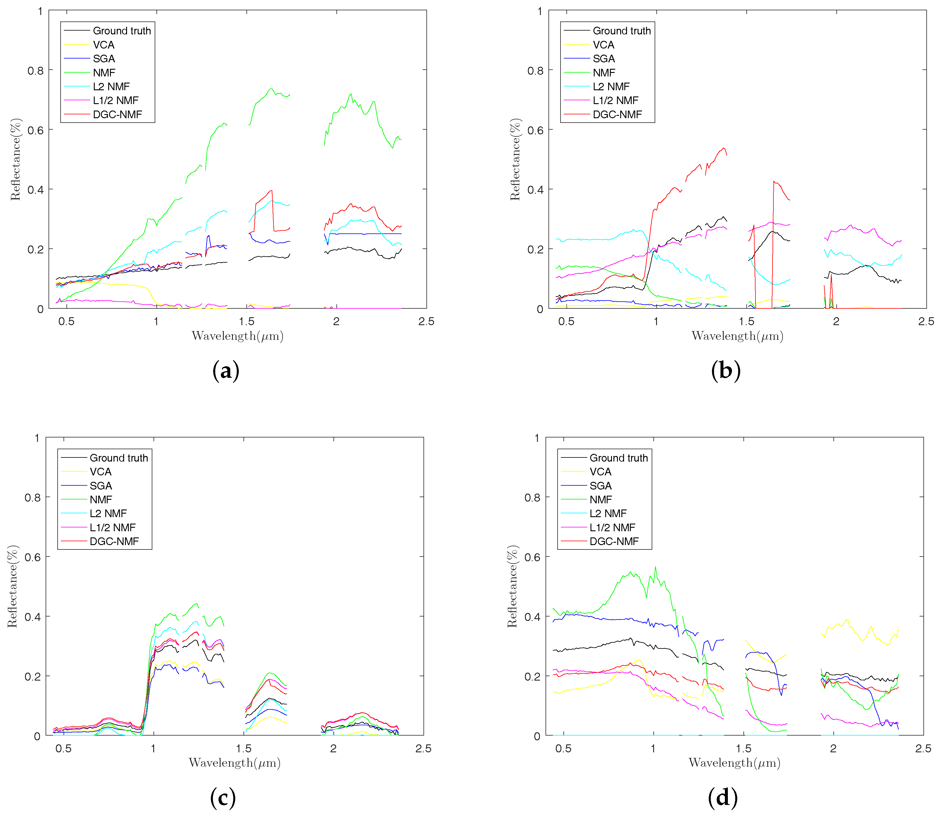
Figure 12.
Comparison of endmember signatures estimated by different methods over urban data. (a) asphalt; (b) grass; (c) trees; (c) roofs. VCA: vertex component analysis; SGA: simplex growing algorithm.
Figure 12.
Comparison of endmember signatures estimated by different methods over urban data. (a) asphalt; (b) grass; (c) trees; (c) roofs. VCA: vertex component analysis; SGA: simplex growing algorithm.

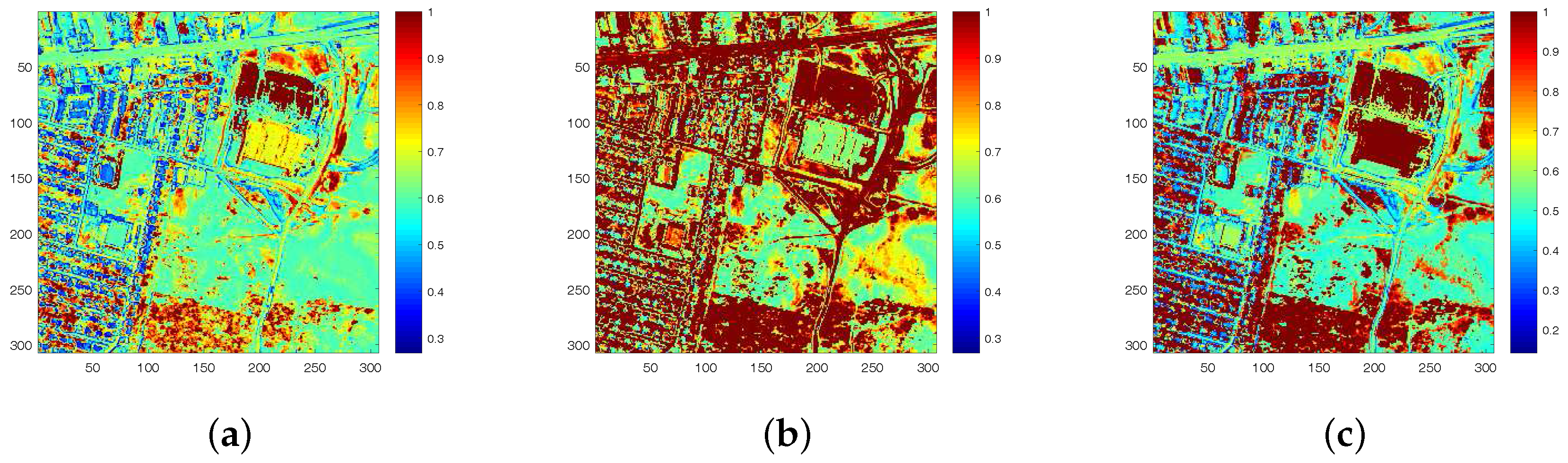
Figure 13.
The sparseness maps of abundance results obtained by different algorithms. (a) -NMF; (b) -NMF; (c) DGC-NMF.
Figure 13.
The sparseness maps of abundance results obtained by different algorithms. (a) -NMF; (b) -NMF; (c) DGC-NMF.

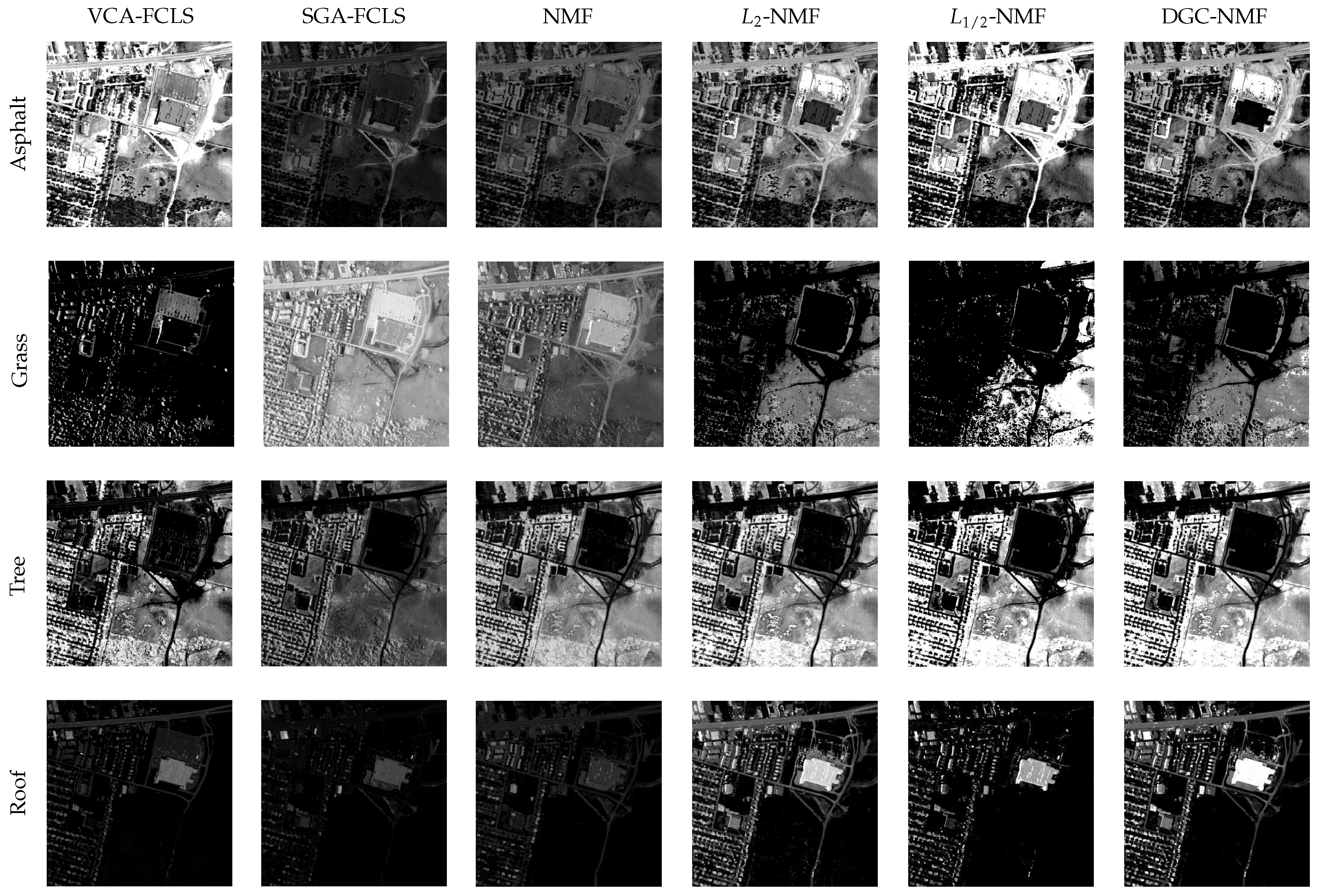
Figure 14.
Abundance maps of urban data estimated by VCA-FCLS, SGA-FCLS, NMF, -NMF, -NMF, and DGC-NMF, respectively, from right column to left column. Each row shows the corresponding abundance maps of a same endmember.
Figure 14.
Abundance maps of urban data estimated by VCA-FCLS, SGA-FCLS, NMF, -NMF, -NMF, and DGC-NMF, respectively, from right column to left column. Each row shows the corresponding abundance maps of a same endmember.

Figure 15.
The extracted endmembers by DGC-NMF and their corresponding United States Geological Survey (USGS) library signatures, along with the estimated abundance maps. (a) alunite; (b) andradite; (c) buddingtonite; (d) dumortierite; (e) kaolinite #1; (f) kaolinite #2; (g) muscovite; (h) montmorillonite; (i) nontronite; (j) pyrope; (k) sphene; and (l) chalcedony.

Table 1.
Comparison of the time cost of different algorithms.
| NMF | L2-NMF | L1/2-NMF | DGC-NMF |
|---|---|---|---|
| 7.61 s | 7.68 s | 8.66 s | 18.80 s |
Table 2.
The spectral angle distance and their standard deviations of algorithms on the urban dataset. Numbers in bold and red color represent the best results, numbers in bold and blue color represent the second-best results. FCLS: full constrained least squares.
Table 2.
The spectral angle distance and their standard deviations of algorithms on the urban dataset. Numbers in bold and red color represent the best results, numbers in bold and blue color represent the second-best results. FCLS: full constrained least squares.
| Endmember | Spectral Angle Distance (10−2) | |||||
|---|---|---|---|---|---|---|
| VCA-FCLS | SGA-FCLS | NMF | L2-NMF | L1/2-NMF | DGC-NMF | |
| Asphalt | 21.04 ± 3.64 | 13.16 | 32.33 | 23.04 | 96.14 | 20.82 |
| Grass | 36.95 ± 0.28 | 109.21 | 124.92 | 81.87 | 36.06 | 51.53 |
| Trees | 28.38 ± 7.78 | 7.43 | 10.19 | 15.93 | 12.70 | 10.07 |
| Roofs | 77.01 ± 0.07 | 21.74 | 39.54 | 138.98 | 38.94 | 6.20 |
| Mean | 40.84 ± 2.87 | 37.89 | 51.75 | 64.96 | 45.96 | 22.16 |
Table 3.
RMSEs and their standard derivations of algorithms on the urban dataset.
| Endmember | Root Mean Square Error (10−2) | |||||
|---|---|---|---|---|---|---|
| VCA-FCLS | SGA-FCLS | NMF | L2-NMF | L1/2-NMF | DGC-NMF | |
| Asphalt | 42.42 ± 12.41 | 30.63 | 23.68 | 32.23 | 41.79 | 20.72 |
| Grass | 47.46 ± 1.23 | 47.19 | 39.00 | 48.24 | 50.00 | 36.57 |
| Trees | 26.92 ± 11.79 | 26.96 | 23.05 | 19.36 | 27.66 | 21.23 |
| Roofs | 18.33 ± 2.00 | 19.40 | 20.30 | 24.18 | 8.84 | 15.08 |
| Mean | 33.78 ± 6.86 | 31.05 | 26.51 | 31.00 | 32.07 | 23.40 |
Table 4.
The spectral angle distance and their standard derivations of algorithms on the Cuprite data. Numbers in bold and red color represent the best results; numbers in bold and blue color represent the second-best results.
Table 4.
The spectral angle distance and their standard derivations of algorithms on the Cuprite data. Numbers in bold and red color represent the best results; numbers in bold and blue color represent the second-best results.
| Endmember | Spectral Angle Distance (10−2) | |||||
|---|---|---|---|---|---|---|
| VCA-FCLS | SGA-FCLS | NMF | L2-NMF | L1/2-NMF | DGC-NMF | |
| Alunite | 17.85 ± 9.39 | 11.05 | 10.03 | 10.18 | 16.01 | 9.91 |
| Andradite | 8.21 ± 2.29 | 8.44 | 13.12 | 7.65 | 12.48 | 12.17 |
| Buddingtonite | 9.82 ± 2.33 | 11.27 | 6.71 | 9.10 | 8.24 | 8.97 |
| Dumortierite | 13.36 ± 3.56 | 13.65 | 13.19 | 10.37 | 6.84 | 10.71 |
| Kaolinite #1 | 7.68 ± 0.18 | 17.90 | 7.33 | 10.88 | 6.88 | 6.40 |
| Kaolinite #2 | 9.82 ± 2.35 | 7.00 | 8.87 | 9.50 | 8.37 | 14.02 |
| Muscovite | 16.51 ± 7.09 | 8.72 | 10.05 | 10.47 | 20.31 | 10.42 |
| Montmorillonite | 11.07 ± 4.63 | 6.81 | 6.42 | 8.76 | 5.89 | 5.88 |
| Nontronite | 7.48 ± 0.15 | 13.39 | 12.53 | 10.52 | 10.90 | 8.69 |
| Pyrope | 9.30 ± 3.25 | 14.69 | 25.36 | 15.67 | 6.24 | 6.12 |
| Sphene | 10.30 ± 5.48 | 23.64 | 5.58 | 65.07 | 28.27 | 24.23 |
| Chalcedony | 12.31 ± 5.22 | 11.66 | 13.20 | 12.62 | 12.28 | 12.41 |
| Mean | 11.14 ± 3.83 | 12.35 | 11.03 | 15.07 | 11.89 | 10.83 |
© 2017 by the authors. Licensee MDPI, Basel, Switzerland. This article is an open access article distributed under the terms and conditions of the Creative Commons Attribution (CC BY) license (http://creativecommons.org/licenses/by/4.0/).
Share and Cite
MDPI and ACS Style
Huang, R.; Li, X.; Zhao, L. Nonnegative Matrix Factorization With Data-Guided Constraints For Hyperspectral Unmixing. Remote Sens. 2017, 9, 1074. https://doi.org/10.3390/rs9101074
AMA Style
Huang R, Li X, Zhao L. Nonnegative Matrix Factorization With Data-Guided Constraints For Hyperspectral Unmixing. Remote Sensing. 2017; 9(10):1074. https://doi.org/10.3390/rs9101074
Chicago/Turabian StyleHuang, Risheng, Xiaorun Li, and Liaoying Zhao. 2017. "Nonnegative Matrix Factorization With Data-Guided Constraints For Hyperspectral Unmixing" Remote Sensing 9, no. 10: 1074. https://doi.org/10.3390/rs9101074
Note that from the first issue of 2016, this journal uses article numbers instead of page numbers. See further details here.