Two-Dimensional Linear Inversion of GPR Data with a Shifting Zoom along the Observation Line
by
 , ,
, ,
Raffaele Persico
1,2,*, 
Giovanni Ludeno
3,
Francesco Soldovieri
3,
Albéric De Coster
4 and
Sébastien Lambot
4 1
Institute for Archaeological and Monumental Heritage IBAM-CNR, Lecce 73100, Italy
2
International Telematic University Uninettuno UTIU, Rome 00186, Italy
3
Institute for the Electromagnetic Sensing of the Environment IREA-CNR, Napoli 80124, Italy
4
Earth and Life Institute, Environmental Sciences, Université catholique de Louvain, Louvain-la-Neuve 1348, Belgium
*
Author to whom correspondence should be addressed.
Remote Sens. 2017, 9(10), 980; https://doi.org/10.3390/rs9100980
Submission received: 23 May 2017
/
Revised: 9 September 2017
/
Accepted: 13 September 2017
/
Published: 22 September 2017
(This article belongs to the Special Issue Radar Systems for the Societal Challenges)
Abstract
:Linear inverse scattering problems can be solved by regularized inversion of a matrix, whose calculation and inversion may require significant computing resources, in particular, a significant amount of RAM memory. This effort is dependent on the extent of the investigation domain, which drives a large amount of data to be gathered and a large number of unknowns to be looked for, when this domain becomes electrically large. This leads, in turn, to the problem of inversion of excessively large matrices. Here, we consider the problem of a ground-penetrating radar (GPR) survey in two-dimensional (2D) geometry, with antennas at an electrically short distance from the soil. In particular, we present a strategy to afford inversion of large investigation domains, based on a shifting zoom procedure. The proposed strategy was successfully validated using experimental radar data.

1. Introduction
The classical way to achieve reliable and well-focused ground-penetrating radar (GPR) images is based on the migration procedure widely used and implemented in most available codes [1,2]. This data processing method originates from seismology [3,4,5], and was later also adapted for the solution of inverse problems in Maxwell′s equations [6,7].
Another class of reconstruction approaches, also deployed in real world applications, exploits linear models of electromagnetic scattering [6]. Either way, the adoption of linear models entails few limitations with regards to the possibility of dealing with mutual interactions between targets [8] and reconstructing the electromagnetic properties of a target in a quantitative way [9]. On the other hand, the Born Approximation method can be extended to a quadratic approximation, which permits mitigation of the effect of non-linearity, in terms of false solution occurrences [10]. The reliability of the inverse scattering approach based on quadratic approximation has been also validated with data collected in the laboratory [11].
Relative to non-linear methods, linear models allow reliable algorithms, based on the minimization of a cost function, which are not affected by the false solutions issue [10,11,12]. The stability of the inversion approach is ensured by the exploitation of regularization schemes. Linear electromagnetic scattering inversion algorithms have been developed and analyzed in relation to their effectiveness with GPR problems and other electromagnetic geo-sounding techniques [13,14,15,16,17]. In addition, linear inverse scattering models have applications in other, non-conventional configurations, such as the “differential ones” [18,19] and for radar on airborne vehicles [20] and UAV [21].
Relative to migration algorithms, a linear inverse scattering approach is able to account, in a rigorous way, for different issues, such as the presence of targets in the near field of the GPR system, truncation of the measurement domain and possible losses in the soil (often ignored in a migration algorithm, or rather counteracted with the application of some gain variable vs. depth). On the other hand, the linear inverse scattering approach requires filling and performing the inversion (in a generalized and regularized sense) of the matrix—which is the discretized version of the linear integral scattering operator—and this can be computationally demanding. The most popular approaches for regularizing a linear inversion are the Truncated Singular Value Decomposition (TSVD) [22,23,24,25] and the Tikhonov method [26]. In this paper, we adopt a TSVD scheme, which permits, relative to migration, a more rigorous analysis of the performance of the inversion approach, in terms of its resolution limits. However, as previously mentioned, it has the main drawback of being much more demanding in terms of computational cost. Consequently, in real GPR surveys (with scanning lines of several tens or even hundreds of wavelengths long), it is not possible to compute SVD for the relatively large matrices involved. This, in general, prevents the possibility of “inverting” an entire radar image in a single step. The first strategy introduced to counteract this issue was to subdivide the overall scan profile into adjacent sub-profiles, sufficiently small enough to allow for the inversion of the matrix, and then, to join the inversion results achieved for each sub-profile side-by-side [27,28]. However, this approach poses several problems (described in detail in Section 4) with regards to the targets located in the proximity of the lateral edges of two adjacent sub-profiles, or those that cross these lateral edges. A strategy aimed at mitigating these issues was presented in [29], where a double sequence of investigation domains was exploited with a shift of half an investigation domain between two successive sub-profiles. In this paper, we propose an extension of that method, referred to as a shifting zoom, aimed at mitigating the problem of the reduction in size of the investigation domain which is needed to perform a sequential linear inversion. The method is validated by processing radar data collected in laboratory conditions over a sand box with three pipes buried at different depths.
The paper is organized as follows: in the next section, we provide the mathematical formulation for the inverse scattering problem. Then, a numerical analysis of the effect of prolongation of the observation line in the parity of the investigation domain is proposed in Section 3. In Section 4, we present the proposed shifting zoom procedure. In Section 5 its effectiveness is shown vs. experimental data, followed by our conclusions.
2. Formulation of the Inverse Scattering Problem
The problem at hand inserts into the framework of microwave tomography from GPR data, which has been largely investigated in the literature, both from the point of view of the imaging algorithms [30,31,32,33] and from the point of view of the effects of the soil and antennas on the data [34,35,36]. Applications to cases in the field have been also presented, e.g., in [37,38].
Here, we briefly report a mathematical formulation that describes a well-known model based on the Born approximation. In particular, the problem at hand concerns a two-dimensional (2D) case with a homogenous background scenario. Under the Born inverse model, a linear integral relationship relates the backscattered electric field (Es) to the unknown contrast function (χ). This contrast function is defined as the relative difference between the (complex) permittivity of the target and the reference scenario. Under the here considered multi-monostatic/multi-frequency configuration, such a relationship is given by:
where G denotes a Green′s function, Einc is the incident field and is the wave number in the relevant medium. In this specific case, the incident field is modeled as the field radiated by a filamentary line source, fed by a unitary electric current located at ro. Λ is the investigated domain, i.e., the spatial region where we assume that the targets reside, whereas the subscript denotes the observation point, belonging to the observation domain.
Here, we make use of a homogeneous reference scenario, and deal with a 2D scalar case. The measurement configuration is multi-monostatic. Consequently, Equation (1) can be specialized as:
where denotes a Hankel function of second kind and zero order. Indeed, a theoretically more correct formulation could be done with the Green’s function of a half-space, as done in [18]. However, the Green’s function of a homogeneous medium (a world “done of soil”) performs accurately enough (especially if the antennas are shielded, which is the case for the experimental data exploited in this paper), and is computationally more efficient than the Green’s function of a half-space. The right-hand side of Equation (2) defines the linear operator (L), relating the unknown contrast function to the scattered field data. The linear integral operator (L) can be expressed in terms of its Singular Value Decomposition (SVD). Hence, σn is the n-th singular value, and vn and un are the n-th left and right singular functions of the operator (L). It is worth noting that {vn} and {un} define the orthonormal basis for the object space, and the data space, respectively [13,22]. A formal solution of the inverse scattering problem is provided by [13,22]:
The ill-posed nature of the inverse problem imposes the adoption of a regularization scheme. A regularized solution is achieved here by using the Truncated SVD (TSVD):
where the regularization parameter is the truncation index (T) in the finite summation Equation (4).
3. The Effect of the Extension of the Observation Line beyond the Investigation Domain
This section is devoted to dealing with the advantages and drawbacks of the extent of the observation domain, with regards to having a fixed extent for the investigation domain. As will be shown, these advantages (if any) are practically quite limited when the observation line becomes longer relative to that of the investigation domain, and when the investigation domain is in the order of a few wavelengths. This provides the basis for the shifting zoom shown in the next section, which is essentially based on the choice of equally long investigation and observation domains.
In particular, the theoretical improvement achievable by prolonging the observation domain over the investigation one, can be seen in terms of the increase in the angle of view, under which the targets are seen, with a consequent improvement in resolution limits [6]. This can be quantified by evaluating the following figure of merit, which represents the energy kernel of the integral equation, integrated across the investigation and observation domains.
This quantity can be expressed in terms of the SVD as the summation of the squares of the singular values of the operator, as follows:
As shown in Appendix A, a physical interpretation can be provided for the summation of the squared singular values; in particular, the quantity Equation (6) accounts for the integral over the investigation domain, for the energy of the images in the Point Spread Function, for each generic point in the investigation domain. Therefore, such a figure of merit allows us to account (in a global way) for the effect of prolongation of the observation domain, in terms of the possibility of capturing the scattered field from the targets in the investigation domain.
Here, we consider an evaluation of the figure of merit (in Equation (6)), for the same matrix exploited later on to process the experimental data. In particular, we are concerned with a propagation medium with a relative dielectric permittivity equal to 2.37. The working frequency band is 800–4000 MHz. The investigation domain has a horizontal extent equal to 0.8 m and a vertical depth of 0.8 m (starting from zero). For the considered depth of the investigation domain, and dielectric permittivity of the medium, it is possible to show that a frequency step of 100 MHz is sufficient, in order to avoid aliasing problems in the inversion [6], and to provide a sufficient time range. The spatial step of the data is 0.01 m.
Now, we consider four different observation domains, with extents of 0.8 m, 1.2 m, 1.6 m and 2.4 m. The relative investigation domains are centred with respect to the observation domain and are sized 0.8 × 0.8 m2 at all times.
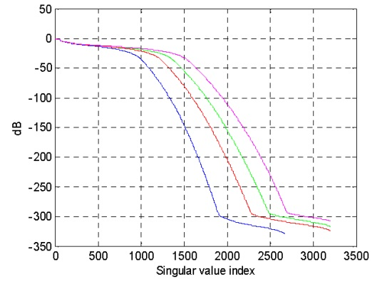
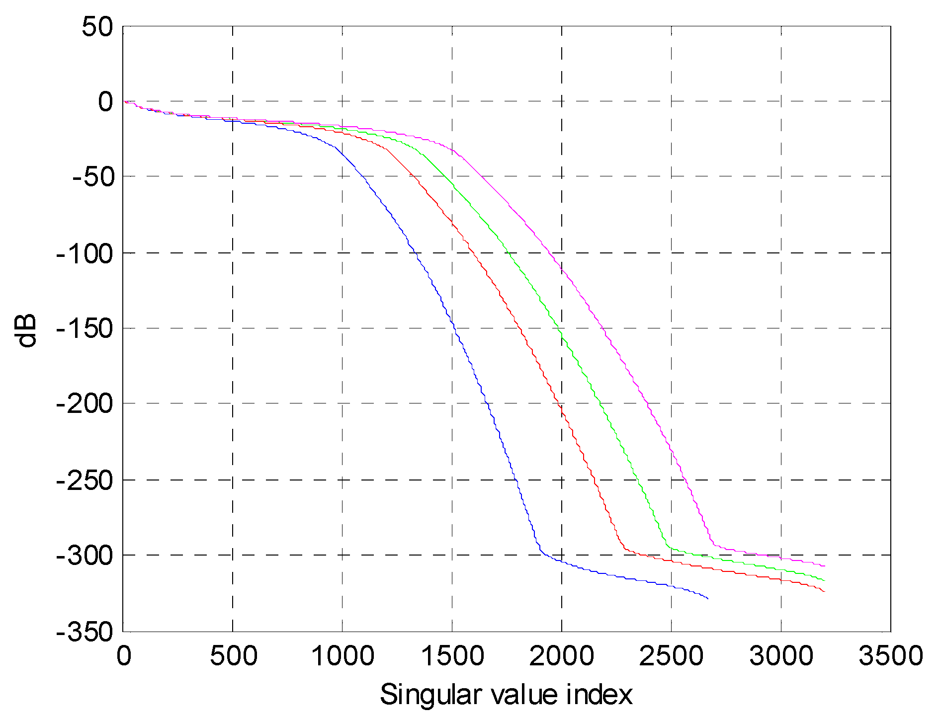
The singular values’ behaviours, relative to the four observation domains, are depicted in Figure 1. It can be noted that there is only a smooth increase in the significant number of singular values for the considered threshold values of TSVD in the reconstruction, and that the curve tends to “saturate”.
The quantities (in Equation (6)) relative to four different cases are reported in Table 1. The second column reports the sum of all squared singular values for the four observation domains. The other two columns report the summation of a finite number of terms; in particular, we consider singular values larger than −20 dB and −30 dB, relative to the maximum one. All the figures are normalised relative to the quantity evaluated for the largest observation domain in Equation (6) (240 cm).
Table 1 shows us that when making the observation domain at hand three times larger, the energy kernel of the operator increases by only about 20%. The physical reason for this is that when we progressively enlarge the observation line in the parity of the investigation domain, this entails a progressively marginal (and vanishing) increase of the maximum geometrical view angle, under which the investigation domain is seen, and on the other hand there is also a progressive decrease in the received signal. In other words, it is illusory to consider achieving a meaningful quantity of extra information about a given target to prolong the observation line indefinitely, even in a lossless case, or even to neglect the effect of the radiation pattern of the antennas, as done in this analysis. Incidentally, to make the simulation more realistic, one should consider an effective or equivalent maximum view angle, customarily smaller than the geometrical maximum view angle (unless a very short observation domain is considered), and influenced by the losses and the directivity characteristics of the antennas; however, this would further enforce the retrieved conclusions.
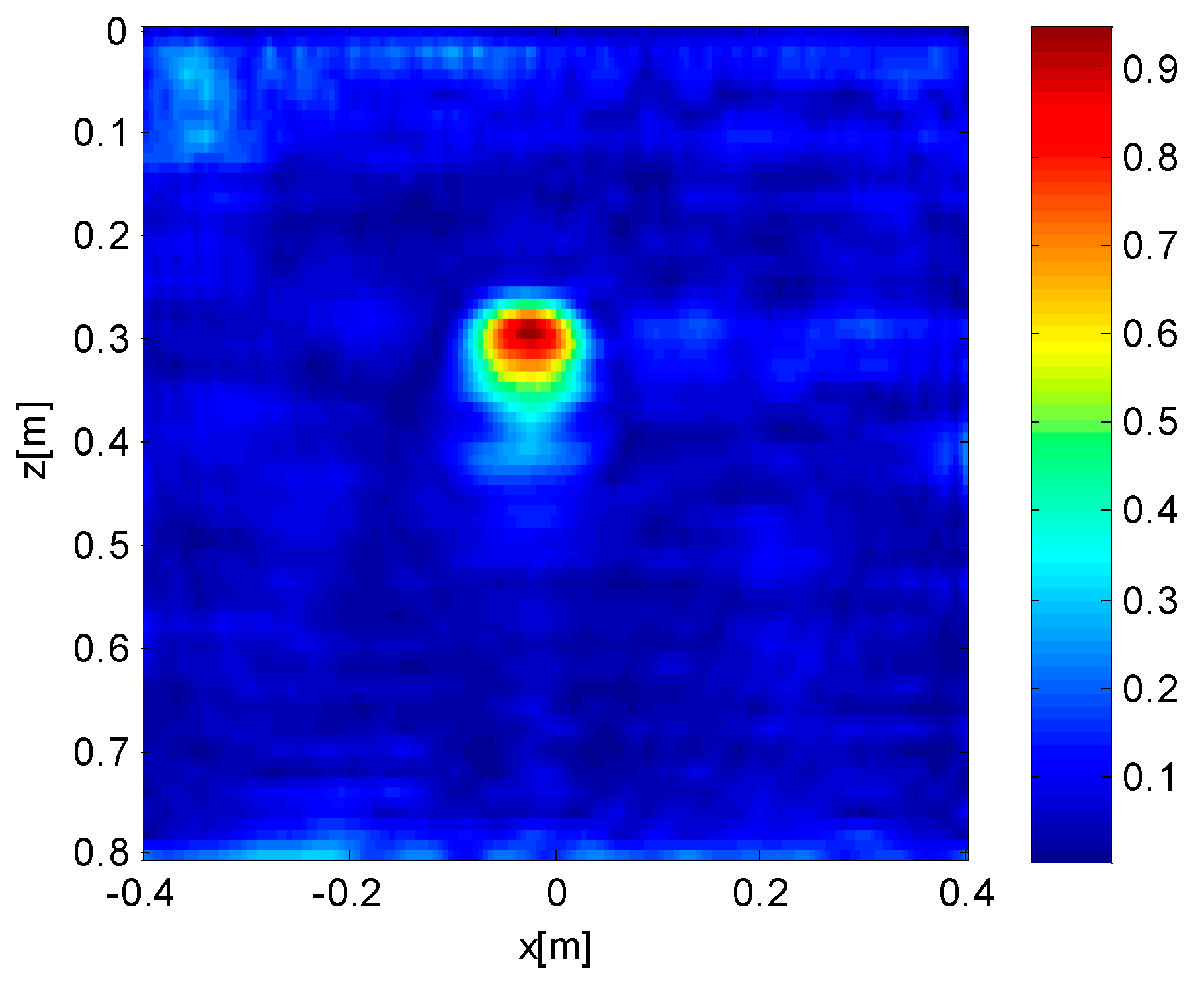
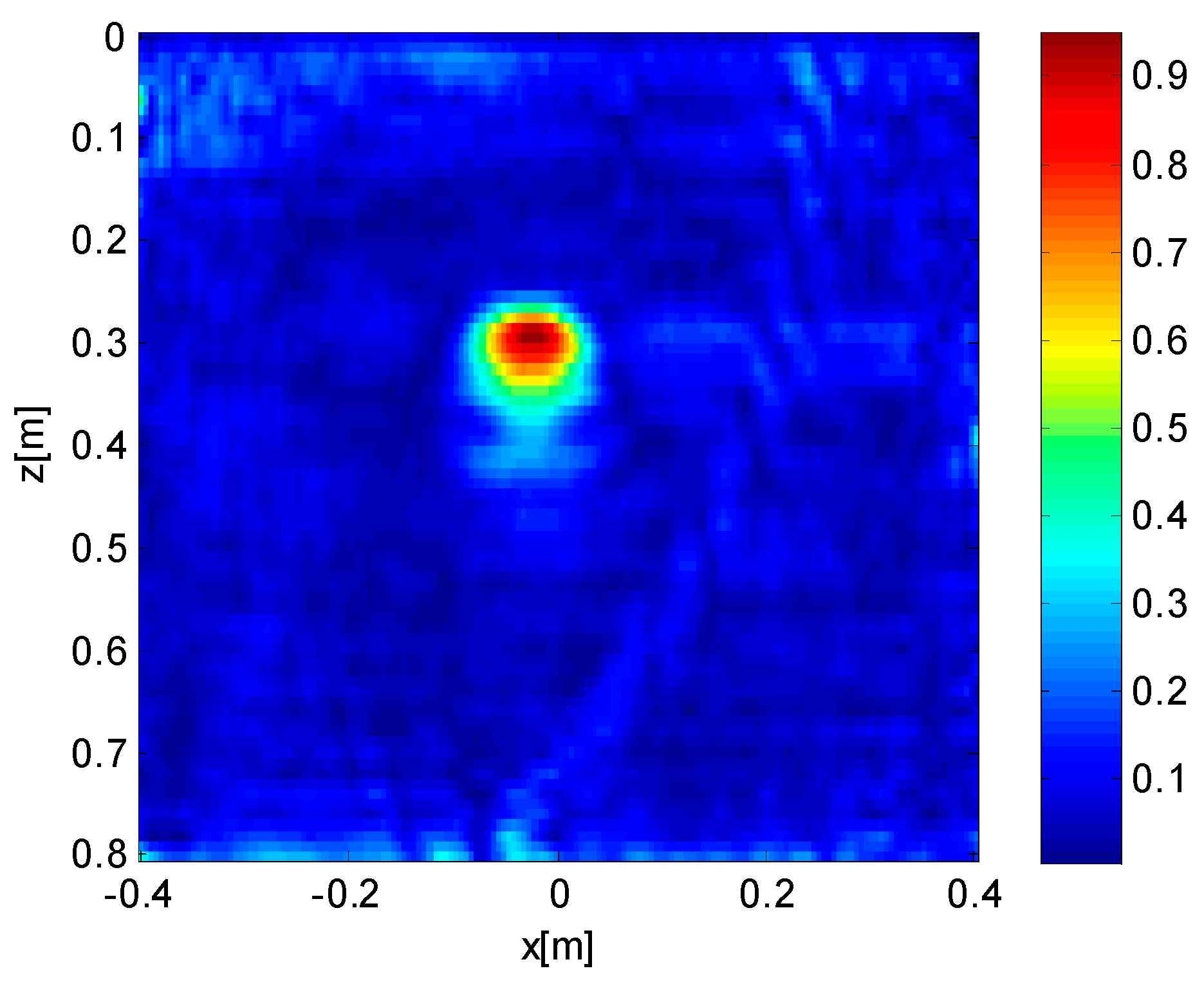
In order to show the negligible effect of an indefinite prolongation of the observation domain in terms of retrievable information, we consider a reconstruction of the central target, embedded in the investigation domain, sized 0.8 × 0.8 m for different extents of the observation domain (0.8, 1.2, 1.6, 2.4 m), under a TSVD with a threshold of −30 dB. The simulated target is a circle made of a perfect electrical conductor, at a depth of 25 cm. The radius of the circle is 5 cm.
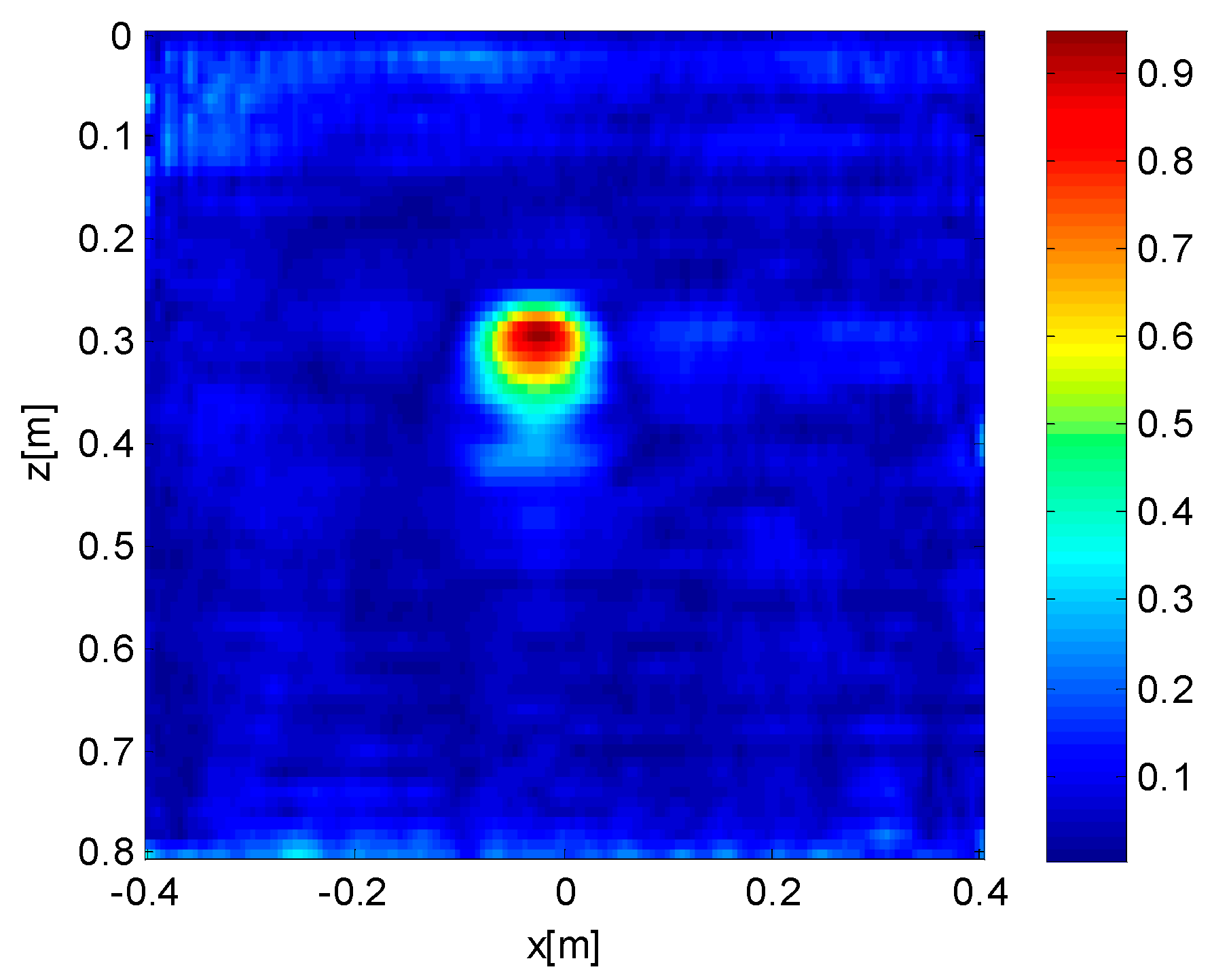
Figure 2, Figure 3, Figure 4 and Figure 5 depict the reconstruction of the target, with observation domain extents equal to 0.8, 1.2, 1.6 and 2.4 m, respectively. As can be seen, progressive enlargement of the observation domain does not improve the reconstruction of the target, which is predominantly the same for all the considered extents. On the other hand, the effects of possible targets outside the chosen investigation domain, in real cases, can produce artifacts. For this reason, from now on we will adopt observation domains of the same length as the relative investigation domains and superpose them.
4. The Shifting Zoom
In the previous section, we showed that the most convenient choice for performing the inversion of a buried area is, in most cases (except for an electrically short observation line that is customarily of no practical interest), to adopt an investigation domain as large as the superposed observation line, and not shifted with respect to it. Consequently, in order to invert a long investigation domain, not viable for a “one-step” inversion, the most natural choice is to adopt subsequent adjacent investigation–observation domains along the radar profile, as schematically indicated in Figure 6. However, this introduces the problem of having targets that might be peripheral to the investigation domain wherein they are located, in particular, with regards to Figure 6 and the observation line (L2), target c is not seen under a symmetric maximum view angle (it is peripheral relative to the observation line, L2), whereas target a is able to cause artefacts in the investigation domain (D2), because it is quite probably perceived by the antennas when they pass the left edge of L2. We also clearly understand that the problem of the peripheral targets, and the problem of the interference for external targets, are two sides of the same coin. In particular, target a is peripheral to D1 and target c is a possible source of artefacts in D3. This last effect is essentially due to the fact that when adopting any fixed investigation domain, we are implicitly assuming that no target is present outside it, which does not correspond, in general, to the ground truth. These problems are clearly related to the performed subdivision into adjacent subdomains. In fact, neither a, nor c, are peripheral targets to the comprehensively gathered profile. The proposed scheme also encompasses the case of a target that crosses the edge between two adjacent domains; in fact, such a target can be ideally seen as a couple of adjacent targets—one on the left-hand side and one on the right-hand side of the edge.
Here, we propose a strategy to overcome this problem, resorting to a more refined definition of consecutive investigation domains. The proposed method is illustrated in Figure 7, and simply consists of retaining the central belt of the current investigation domain. Then, the subsequent investigation domain is shifted by the same amount, relative to the previous one, so that we do not have consecutive adjacent investigation domains, but rather, consecutive overlapping investigation domains. For example, in Figure 7, the generic kth investigation domain is indicated in red, and its central belt is coloured in red too. The homologous areas with respect to the (k + 1)th investigation domain are labelled in green. Also, the observation lines have to be coherently shifted, to keep them hanging on the relative underlying investigation domains, as indicated in Figure 7. In order to guarantee continuous hanging between the current investigation and observation domains, it is necessary for the horizontal extent of the pixels in the representation of the reconstruction to be an entire multiple, or an entire sub-multiple, of the spatial step of the measures. This can be achieved by means of a proper choice of the size of the pixels, or alternatively, by means of some interpolation, either on the measurement points, or in the representation of the current reconstruction.
Please note that in Figure 7, the overall observation line is indicated with L, and the indications of Lk and Lk+1 indicate subsets of L; they are represented at different heights just to allow us to distinguish them from each other.
There is some degree of arbitrariness in defining the central belt of the current reconstruction, but we can think of it just as a piled sequence of centred pixels for the final kth reconstruction. In particular, the result from the current inversion is represented by a matrix, A(i,j), with n × m pixels, and the central belt can be defined as the column, A(i, (m + 1)/2), i = 1…n, if m is odd, or as two columns A(i, (m/2)) and A(i, (m/2) + 1), if m is even. Clearly, with a shifting zoom, the joined reconstructions are relative to the central belts of observation domains. Consequently, no peripheral target is created beyond those that are “naturally peripheral”, i.e., placed at the beginning or towards the end of the comprehensively gathered B-scan. At the same time, the undesired effects of targets immediately external to the current observation–investigation domain are made negligible, because these targets are clearly distant from the central belt of the investigation domain. That said, however, for a complete representation of the processed available image, it is necessary that the left half of the first investigation domain (before the “first central belt”) and the right half of the last investigation domain (after the “last central belt”) are joined to the reconstruction. In this way, no datum, and no piece of the available information is lost. Of course, in this way, the initial or final targets are “physically peripheral” with respect to the gathered profile, and some targets before or after the physically gathered B-scan might create artefacts. However, these are unavoidable physical phenomena, not drawbacks related to the adopted inversion technique—the shifting zoom just avoids these drawbacks propagating throughout the entire GPR profile.
5. Experimental Results
This section is devoted to presenting the data and the results of the processing performed on them, with and without a shifting zoom. The exploited GPR system consisted of a vector network analyzer (VNA), which comprised a stepped-frequency continuous-wave (SFCW) radar system (ZVRE, Rohde & Schwarz, Munich, Germany) and a linearly polarized, double-ridged broadband horn antenna (BBHA 9120 A, Schwarzbeck Mess-Elektronik, Schönau, Germany) as the simultaneous transmitter and receiver. The antenna dimensions were as follows: height, 195 mm; aperture, 142 × 245 mm. The antenna nominal frequency range was 0.8 to 5.0 GHz and its isotropic gain ranges were from 6 to 18 dB. The relatively high directivity of the antenna (45°, 3 dB beam width in the E-plane and 30° in the H-plane at 1 GHz) made it immune to interferences from external sources or reflectors. The antenna was connected to the reflection port of the VNA via a high-quality N-type 50-Ohm coaxial cable.
We calibrated the VNA at the connection between the antenna feed point and the cable using an Open-Short-Match calibration kit. The frequency-dependent complex ratio (S11(f)) between the backscattered waves and the incident waves at the radar reference plane was measured at 1601 frequencies over a range of 800 to 4000 MHz, with a frequency step of 2 MHz.
The radar measurements were performed over a 3 × 3 m sand box, with the antenna aperture situated at about 1 cm above the sand surface. A copper sheet, assumed as a perfect electrical conductor (PEC), was installed at the bottom of the 0.86 m thick sand layer, to control the boundary conditions. The targets were three PVC pipes, 1.20 m in length and 50 mm in diameter, with a thickness of 1.8 mm, and were buried at depths of 0.07, 0.29, and 0.51 m, respectively. The three pipes were placed parallel to each other, and their horizontal distances from the start point of the B-scans were about equal to 0.47, 1.17 and 1.97 m, respectively. The pipes were filled with air. The radar system was installed on an XYZ automated positioning table to automatically acquire the data over a 2.40 m long profile, with a position step of 1 cm. The radar profile was transverse to the pipes.
In accordance with the near-field radar antenna model of Lambot and André [39], the antenna global reflection and transmission functions were determined. Then, in order to remove a portion of the antenna effects, the free-space response of the antenna was subtracted from S11(f). The frequency-domain radar data were subsequently converted into the time domain, using the inverse Fourier Transform (see Figure 8a), and zero timing with background removal was subsequently applied to highlight the targets (see Figure 8b).
Let us now present some results relative to the entire collected experimental dataset presented in Figure 8. For the inversion, the same measurement/inversion parameters from the example described in the section above were used (in particular, observation and investigation domains were 0.8 m long), because the simulations were calibrated on the basis of the experimental results that had already been achieved beforehand. In particular, the sand was dry and its relative permittivity was estimated from the diffraction hyperbolas to be about equal to 2.37, as previously mentioned. The inversions were performed by means of a numerical TSVD, truncated at −30 dB.
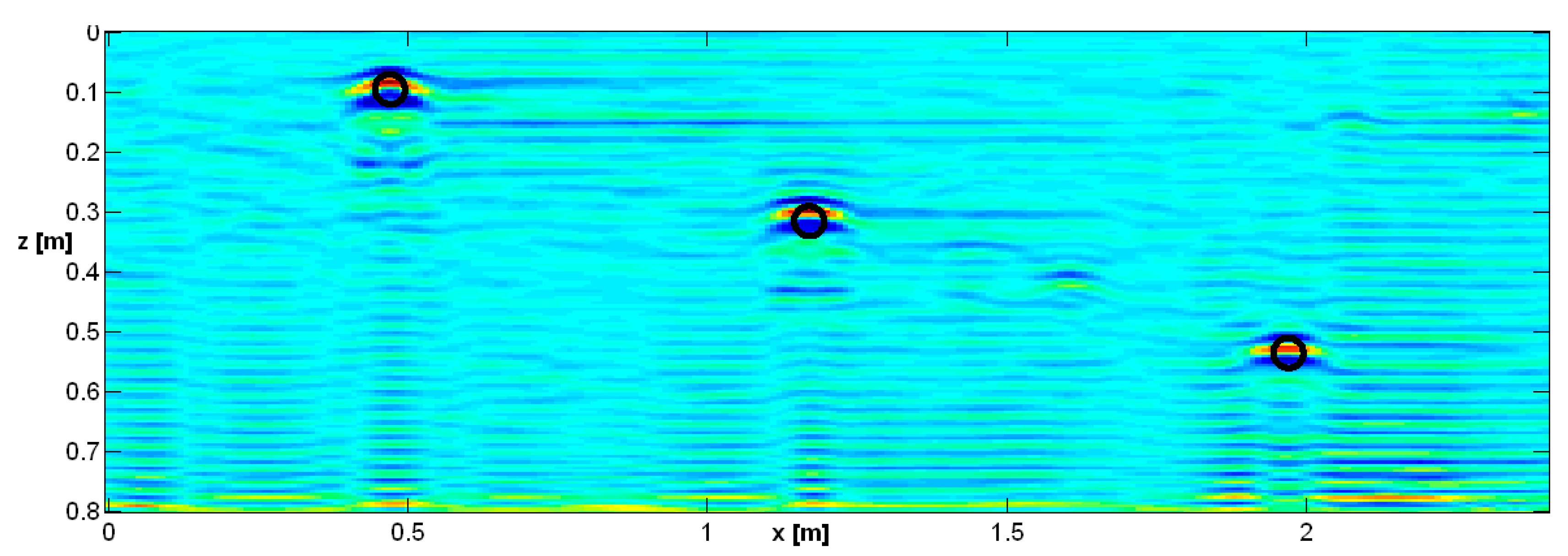
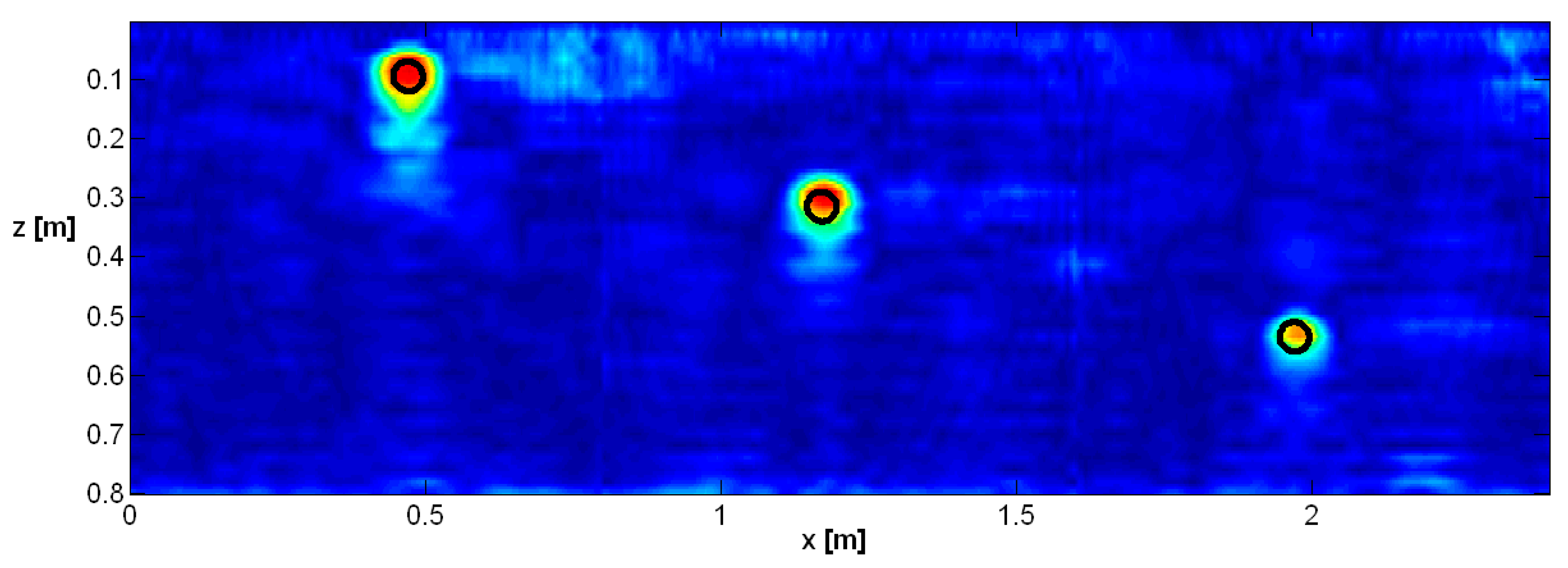
The first result, shown in Figure 9, refers to subdivision of the overall domain, 2.4 m long, into three adjacent observation domains, each of which are 0.8 m long. As can be seen, two boundary lines are visible between the three investigation domains. In Figure 9, and in the following ones, the real cross section of the buried pipes is also depicted.
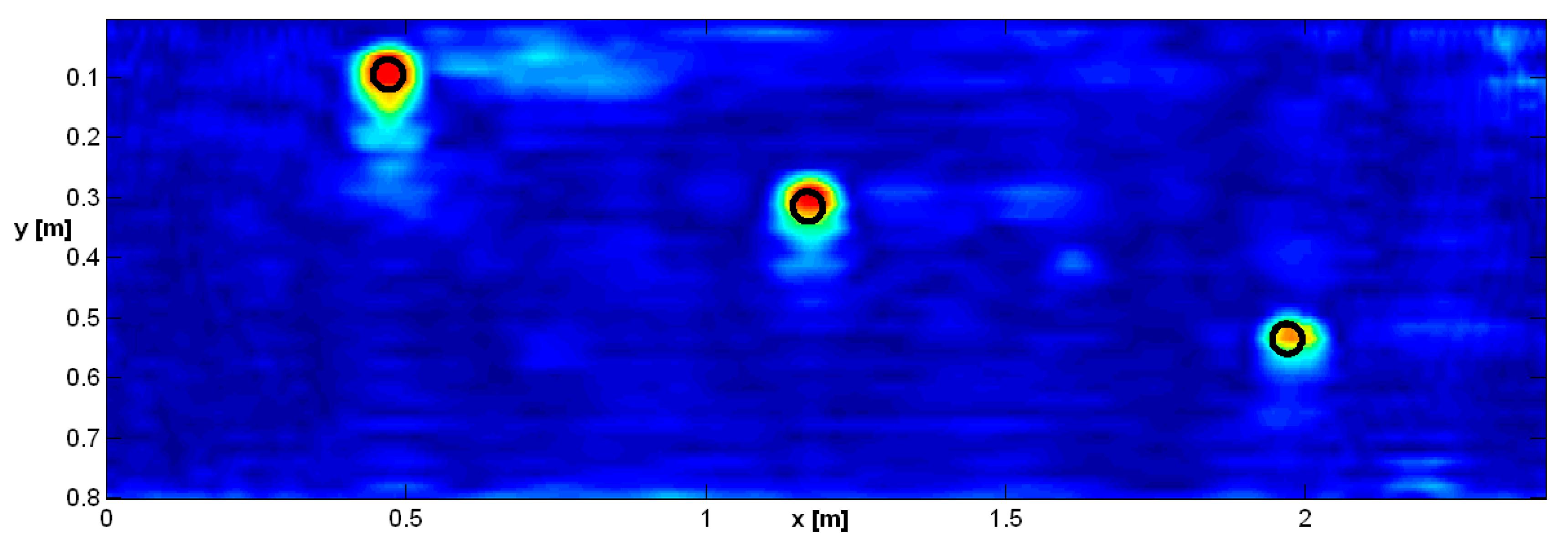
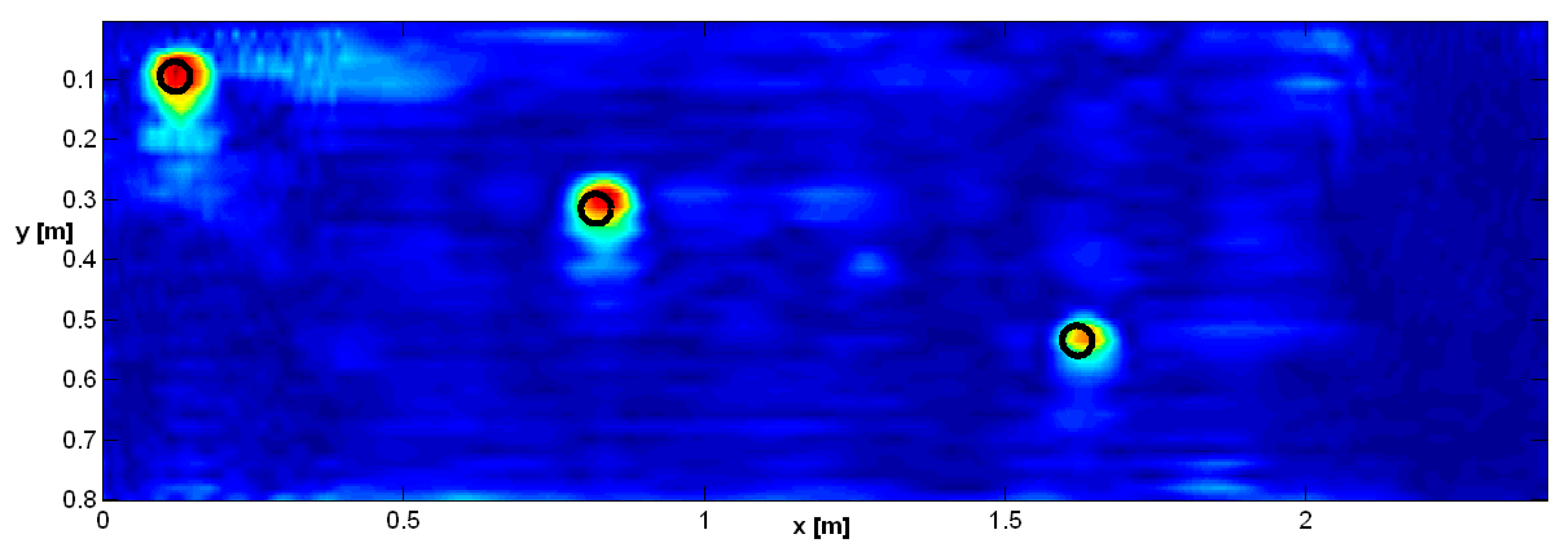
Figure 10 depicts the result when the shifting zoom procedure is applied. It can be seen that the stitching lines disappeared and some artifacts (especially for the investigation domain of the second target) were mitigated.
The effect would be stronger still if the targets were not centered with respect to their relative investigation domains. We simulated such a situation by shifting the starting point of the inverted data 35 cm beyond the initial point of Figure 9 and Figure 10. Then, in order to keep the comprehensive length of the B-scan equal to 240 cm, we fictitiously added identically null data on the right-hand side of the gathered data. In this way, it is as if the targets were pulled 35 cm towards the left-hand side (we could not do this experiment by physically gathering a new B-scan, shifted 35 cm with respect to the previous one, due to the comprehensive size of the sand pool). Then, we inverted the data along three adjacent investigation domains in the same way as adopted for Figure 10. The results are shown in Figure 11. Now, the three targets have become peripheral to the relative investigation domains, and the consequence is some meaningful deformation (particularly evident with respect to the central target and to the right-hand side target, which cross the boundary between two adjacent investigation domains). It can be also appreciated that in Figure 11, the deformations and the artefacts tend to be quite asymmetrical, because the view angles under which the three targets are seen now, are meaningfully asymmetrical. Finally, we applied the shifting zoom to the inversion of the shifted data. The result is shown in Figure 12, and, as shown, the targets are shifted with respect to Figure 9 and Figure 10, but no substantial deformation can be found on the targets, with respect to Figure 9 and Figure 10.
Finally, in Figure 13, the result of a migration performed on the same data of Figure 9 and Figure 10 is reported. Specifically, a Kirchhoff migration was performed on 41 traces, making use of the same relative permittivity (2.37) exploited for the inverse scattering results. The migration was performed by importing the synthetic time data into Reflexw (the previous elaborations were performed by means of homemade MATLAB routines). After migration, the data were re-imported into MATLAB and a time–depth conversion was performed for the representation. It can be seen that the effects of the ringing of the antennas and the effects of the background removal are more visible.
6. Conclusions
In this study, a shifting zoom method was proposed, in order to enable the application of a linear inversion to a long radar image, without suffering from negative effects essentially due to a limited view angle, introduced by the subdivision of the image into smaller subdomains. The shifting zoom extends the method introduced in [29]. Relative to [29], the improvement achieved by the shifting zoom is that the vertical stitches disappear completely, whereas in that work their number was two-fold larger than with adjacent investigation domains. This is due to the fact that the central belt is quite narrow relative to the entire current investigation domain, whereas it was as large as half of the investigation domain in [29]. Consequently, in that case there was a meaningfully different average level between any two adjacent final images. Moreover, under the method explained in [29], the length of the observation line, in general, was not an integer multiple of the width of the chosen investigation domain, and some cases, dependent “manual binding” or zero padding was needed, in order to stitch together the entire data gathered along the observation line. With a shifting zoom, the settings of a number of inversions that guarantee the entire coverage of the gathered observation line can be easily made automatic, and do not require any zero-padding. That said, the different (certainly superior) quality of the results achieved here are also due the larger band of the antennas, the more controlled environmental conditions and the fact that the targets were shallower.
The extra computational burden needed for the shifting zoom with respect to the use of adjacent investigation domains is minimal, because the matrix to be inverted is calculated completely off-line, as is its SVD. What is needed when performing the shifting zoom, is a larger number of matrix-vector products that are fast operators. In particular, calculation of the elements of the matrix and computation of its numerical SVD requires slightly less than two hours, whereas the sequential shifting zoom requires about 30 s. This is the extra time needed in the case at hand. When an extrapolation to possible real-life cases is performed, this means that considering, for example, 60 B-scans, each of which is 24 m long (which means 10 times the B-scan considered here) the time specifically needed for the shifting zoom would be in the order of 30 × 10 × 60 s = 18,000 s = 5 h. This may correspond, for example, to the size of an area of archaeological interest which needs to be probed. The inversion also required some work on the data (inverse Fourier transform in time domain, zero timing, background removal, time cut, Fourier transform again—because the inversion is in the frequency domain), but the required CPU time for this was shorter than 30 s and would not increase meaningfully on larger scales. So, most of the required computational time was devoted to the calculation of the matrix and its SVD, which is the same, either with or without, shifting zoom. Please note that due to the limited available RAM memory, it was impossible to perform a SVD of the matrix corresponding to the entire investigation and observation domains (2.4 m long) with the available computer, which was an ASUS desktop with 2 Gb of RAM. It is worth noting that also a migration is, in general, expressed as an integral weighted summation of the data around a central point, and this means also that a migration, if examined more attentively, is implicitly based on a shifting zoom algorithm. In conclusion, this work proposes a translation in the plane of inversion for a procedure customarily applied to migration algorithms. Future research works will focus on further real radar datasets, possibly on larger scales, to combine the proposed method with the intrinsic, near-field antenna model of Lambot and André [39,40], through which antenna effects will be further filtered out.
Acknowledgments
This project has received funding from the European Union within the Horizon 2020 research and innovation programme under grant agreement No. 700395. Moreover, this work was supported and funded by the Walloon Region through the ”SENSPORT” project (Convention n°1217720) undertaken in the framework of the WBGreen research program. We also benefited from the FNRS-Belgium (Fonds National de la Recherche Scientifique) support and the networking activities carried out within the EU funded COST Action TU1208 ”Civil Engineering Applications of Ground Penetrating Radar”.
Author Contributions
Persico, Ludeno and Soldovieri cured the inversion aspects, Lambot and Decoster assembled and calibrated the exploited stepped frequency GPR, cured the preparation of the test site and gathered the data. All the authors contributes together to the writing and the correction of the paper.
Conflicts of Interest
The authors declare no conflict of interest.
Appendix A
This appendix is devoted to the physical interpretation of the quantity in Equation (6). For the sake of simplicity and generality, we have rewritten the relevant equation in a more general form.
with its SVD provided through the singular value system . The Point Spread Function, for a pulse located at can be expressed as:
and its image in the data space is given by:
The integral
represents the energy of the image of the Point Spread Function for a pulse located at point x′. This quantity can be expressed by exploiting the orthonormality of the functions in the data space as:
Now, if we integrate the quantity over the investigation domain, we obtain the following:
Therefore, the summation of the squared singular values represents the summation of the energies of the images of the Point Spread Function (PSF) for each generic point x′ in the investigation domain. The same consideration holds when regularization is applied by the Truncated Singular Value Decomposition (TSVD), once we consider (in Equation (A6)) the summation truncated at the index (T).
References
- Sandmeier, K.J. Reflexw. Software Catalogue 2009. Available online: www.sandmeier-geo.de/reflexw.html (accessed on 1 August 2016).
- Goodman, D.; Piro, S. GPR and Remote Sensing in Archaeology; Springer: Berlin, Germany, 2013. [Google Scholar]
- Yilmaz, O. Seismic Data Analysis—Processing, Inversion and Interpretation of Seismic Data; Society of Exploration Geophysicists: Tulsa, OK, USA, 2000. [Google Scholar]
- Stolt, R.H. Migration by Fourier Transform. Geophysics 1978, 43, 23–48. [Google Scholar] [CrossRef]
- Schneider, W.A. Integral formulation for migration in two and three dimensions. Geophysics 1978, 43, 49–76. [Google Scholar] [CrossRef]
- Persico, R. Introduction to Ground Penetrating Radar: Inverse Scattering and Data Processing; Wiley: Hoboken, NJ, USA, 2014. [Google Scholar]
- Leuschen, C.J.; Plumb, R.G. A Matched-Filter-Based Reverse-Time Migration Algorithm for Ground-Penetrating Radar Data. IEEE Trans. Geosci. Remote Sens. 2001, 39, 929–936. [Google Scholar] [CrossRef]
- Marengo, E.A. Quasi-Born approximation scattering and inverse scattering of multiple scattering targets. IET Radar, Sonar Navig. 2017, 11, 1276–1284. [Google Scholar] [CrossRef]
- Di Donato, L.; Palmeri, R.; Sorbello, G.; Isernia, T.; Crocco, L. A new linear distorted-wave inversion method for microwave imaging via virtual experiments. IEEE Trans. Microw. Theory Tech. 2016, 64, 2478–2488. [Google Scholar] [CrossRef]
- Raffaele, P.; Francesco, S.; Rocco, P. Convergence Properties of a Quadratic Approach to the Inverse Scattering Problem. J. Opt. Soc. Am. Part A 2002, 19, 2424–2428. [Google Scholar]
- Persico, R.; Bernini, R.; Soldovieri, F. The role of the measurement configuration in inverse scattering from buried objects under the Born approximation. IEEE Trans. Antennas Propag. 2005, 6, 1875–1886. [Google Scholar] [CrossRef]
- Picco, V.; Gennarelli, G.; Negishi, T.; Soldovieri, F.; Erricolo, D. Experimental validation of the quadratic forward model for RF tomography. IEEE Geosci. Remote Sens. Lett. 2015, 12, 1461–1465. [Google Scholar] [CrossRef]
- Catapano, I.; Crocco, L.; Persico, R.; Pieraccini, M.; Soldovieri, F. Linear and Non-linear Microwave Tomography Approaches for Subsurface Prospecting: Validation on Real Data. IEEE Trans. Antennas Wireless Propag. Lett. 2006, 5, 49–53. [Google Scholar] [CrossRef]
- Meinke, P. Linear GPR inversion for lossy soil and a planar air-soil interface. IEEE Trans. Geosci. Remote Sens. 2001, 39, 2713–2721. [Google Scholar] [CrossRef] [Green Version]
- Comite, D.; Ahmad, F.; Liao, D.; Dogaru, T.; Amin, M.G. Multiview imaging for low-signature target detection in rough-surface clutter environment. IEEE Trans. Geosci. Remote Sens. 2017, PP, 1–10. [Google Scholar] [CrossRef]
- Almeida, E.R.; Porsani, J.L.; Catapano, I.; Gennarelli, G.; Soldovieri, F. Microwave tomography-enhanced GPR in forensic surveys: The case study of a tropical environment. IEEE J. Sel. Top. Appl. Earth Obs. Remote Sens. 2016, 9, 115–124. [Google Scholar] [CrossRef]
- Masini, N.; Persico, R.; Rizzo, E.; Calia, A.; Giannotta, M.T.; Quarta, G.; Pagliuca, A. Integrated Techniques for Analysis and Monitoring of Historical Monuments: The case of S.Giovanni al Sepolcro in Brindisi (Southern Italy). Near Surf. Geophys 2010, 8, 423–432. [Google Scholar] [CrossRef]
- Persico, R.; Pochanin, G.; Ruban, V.; Orlenko, A.; Catapano, I.; Soldovieri, F. Performances of a Microwave Tomographic Algorithm for GPR Systems Working in Differential Configuration. IEEE J. Sel. Top. Appl. Earth Obs. Remote Sens. 2016, 9, 1343–1356. [Google Scholar] [CrossRef]
- Persico, R.; Soldovieri, F. A Microwave Tomography Approach for a Differential Configuration in GPR Prospecting. IEEE Trans. Antennas Propag. 2006, 54, 3541–3548. [Google Scholar] [CrossRef]
- Gennarelli, G.; Catapano, I.; Soldovieri, F. Reconstruction Capabilities of Down-Looking Airborne GPRs: the Single Frequency Case. IEEE Trans. Comput. Imaging 2017, PP, 1. [Google Scholar] [CrossRef]
- Ludeno, G.; Catapano, I.; Gennarelli, G.; Soldovieri, F.; Vetrella, A.R.; Renga, A.; Fasano, G. A micro-UAV-borne system for radar imaging: A feasibility study. In Proceedings of the 2017 9th International Workshop on Advanced Ground Penetrating Radar (IWAGPR), Edinburgh, UK, 28–30 June 2017; pp. 1–4. [Google Scholar]
- Bertero, M.; Boccacci, P. Introduction to Inverse Problems in Imaging; Institute of Physics Publishing, Bristol and Philadelphia: Bristol, UK, 1998. [Google Scholar]
- Catapano, I.; Soldovieri, F.; Alli, G.; Mollo, G.; Forte, L.A. On the Reconstruction Capabilities of Beamforming and a Microwave Tomographic Approach. IEEE Geosci. Remote Sens. Lett. 2015, 12, 2369–2373. [Google Scholar] [CrossRef]
- Gennarelli, G.; Catapano, I.; Soldovieri, F.; Persico, R. On the Achievable Imaging Performance in Full 3-D Linear Inverse Scattering. IEEE Trans. Antennas Propag. 2015, 63, 1150–1155. [Google Scholar] [CrossRef]
- Savelyev, T.G.; Van Kempen, L.; Sahli, H.; Sachs, J.; Sato, M. Investigation of time–frequency features for GPR landmine discrimination. IEEE Trans. Geosci. Remote Sens. 2007, 45, 118–129. [Google Scholar] [CrossRef]
- Hidalgo-Silva, H.; Gómez-Treviño, E. Nonsmooth nonconvex optimization for low-frequency geosounding inversion. IEEE J. Sel. Top. Appl. Earth Obs. Remote Sens. 2016, 9, 2197–2205. [Google Scholar] [CrossRef]
- Pettinelli, E.; Di Matteo, A.; Mattei, E.; Crocco, L.; Soldovieri, F.; Redman, D.J.; Annan, A.P. GPR response from buried pipes: Measurement on field site and tomographic reconstructions. IEEE Trans. Geosci. Remote Sens. 2009, 47, 2639–2645. [Google Scholar] [CrossRef]
- Persico, R.; Soldovieri, F.; Utsi, E. Microwave tomography for processing of GPR data at Ballachulish. J. Geophys. Eng. 2010, 7, 164–173. [Google Scholar] [CrossRef]
- Persico, R.; Sala, J. The problem of the investigation domain subdivision in 2D linear inversions for large scale GPR data. IEEE Geosci. Remote Sens. Lett. 2014, 11, 1215–1219. [Google Scholar] [CrossRef]
- Liu, T.; Klotzsche, A.; Pondkule, M.; Vereecken, H.; van der Kruk, J.; Su, Y. Estimation of subsurface cylindrical object properties from GPR full-waveform inversion. In Proceedings of the 2017 9th International Workshop on Advanced Ground Penetrating Radar (IWAGPR), Edinburgh, UK, 28–30 June 2017; pp. 1–4. [Google Scholar]
- Meles, G.A.; Greenhalgh, S.A.; Green, A.G.; Maurer, H.; van der Kruk, J. GPR Full-Waveform Sensitivity and Resolution Analysis Using an FDTD Adjoint Method. IEEE Trans. Geosci. Remote Sens. 2012, 50, 1881–1896. [Google Scholar] [CrossRef]
- Klotzsche, A.; van der Kruk, J.; Niklas, L.; Joseph, D.; Harry, V. 3-D characterization of high-permeability zones in a gravel aquifer using 2-D crosshole GPR full-waveform inversion and waveguide detection. Geophys. J. Int. 2013, 195, 932–944. [Google Scholar] [CrossRef]
- Sun, S.; Kooij, B.J.; Yarovoy, A.G. Linearized 3-D Electromagnetic Contrast Source Inversion and Its Applications to Half-Space Configurations. IEEE Trans. Geosci. Remote Sens. 2017, 55, 3475–3487. [Google Scholar] [CrossRef]
- Soldovieri, F.; Lopera, O.; Lambot, S. Combination of Advanced Inversion Techniques for an Accurate Target Localization via GPR for Demining Applications. IEEE Trans. Geosci. Remote Sens. 2011, 49, 451–461. [Google Scholar] [CrossRef]
- Soldovieri, F.; Persico, R.; Leone, G. Effect of source and receiver radiation characteristics in subsurface prospecting within the DBA. Radio Sci. 2005, 40, RS3006. [Google Scholar] [CrossRef]
- Slob, E.; Fokkema, J. Coupling effects of two electric dipoles on an interface. Radio Sci. 2002, 37, 5. [Google Scholar] [CrossRef]
- Piscitelli, S.; Rizzo, E.; Cristallo, F.; Lapenna, V.; Crocco, L.; Persico, R.; Soldovieri, F. GPR and Microwave Tomography for Detecting shallow Cavities in the Historical Area of Sassi of Matera (Southern Italy). Near Surf. Geophys. 2007, 5, 275–285. [Google Scholar] [CrossRef]
- Leucci, G.; Masini, N.; Persico, R.; Soldovieri, F. GPR and sonic tomography for structural restoration: The case of the Cathedral of Tricarico. J. Geophys. Eng. 2011, 8, S76–S92. [Google Scholar] [CrossRef]
- Lambot, S.; André, F. Full-Wave Modeling of Near-Field Radar Data for Planar Layered Media Reconstruction. IEEE Trans. Geosci. Remote Sens. 2014, 52, 2295–2303. [Google Scholar] [CrossRef]
- De Coster, A.; Lambot, S. Full-Wave Removal of Internal Antenna Effects and Antenna-Medium Interactions for Improved Ground-Penetrating Radar Imaging. IEEE Trans. Geosci. Remote Sens. 2017. under review. [Google Scholar]
Figure 1.
Singular values for increasing observation lines in the parity of the investigation line. The investigation domain is 80 × 80 cm and is centered under the observation line. The observation lines are represented as follows: blue line, observation line, 80 cm long; red line, observation line, 120 cm long; green line, observation line, 160 cm long; cyan line, observation line, 240 cm long. The singular values’ curves are normalized with respect to the maximum singular value.

Figure 2.
Target reconstruction with an observation domain equal to 0.8 m.

Figure 3.
Target reconstruction with an observation domain equal to 1.2 m.

Figure 4.
Target reconstruction with an observation domain equal to 1.6 m.

Figure 5.
Target reconstruction with an observation domain equal to 2.4 m.

Figure 6.
Scheme for the inversion of a long radar image, making use of a sequence of adjacent investigation domains and a relative sequence of observation lines.
Figure 6.
Scheme for the inversion of a long radar image, making use of a sequence of adjacent investigation domains and a relative sequence of observation lines.
Figure 7.
Schematic for the shifting zoom.
Figure 8.
The experimental radar data, in time domains, after free-space response removal (a), and after further (b) zero timing and background removal. In the lower image, a time cut has also been done, in order to focus on the depth range of interest.
Figure 8.
The experimental radar data, in time domains, after free-space response removal (a), and after further (b) zero timing and background removal. In the lower image, a time cut has also been done, in order to focus on the depth range of interest.
Figure 9.
Reconstruction achieved with three adjacent investigation-observation domains (0.8 m long).
Figure 9.
Reconstruction achieved with three adjacent investigation-observation domains (0.8 m long).

Figure 10.
Reconstruction achieved with a shifting zoom. The shifting step is 1 cm, equal to the spatial step of the data, and to the horizontal size of the pixels, for the representation of the reconstruction.
Figure 10.
Reconstruction achieved with a shifting zoom. The shifting step is 1 cm, equal to the spatial step of the data, and to the horizontal size of the pixels, for the representation of the reconstruction.

Figure 11.
Reconstruction achieved with three adjacent investigation-observation domains, under a data shift of 35 cm.
Figure 11.
Reconstruction achieved with three adjacent investigation-observation domains, under a data shift of 35 cm.
Figure 12.
Reconstruction achieved with the shifting zoom, under a data shift of 35 cm.

Figure 13.
Result of a Kirchhoff migraton performed on the same data as in Figure 10.
Figure 13.
Result of a Kirchhoff migraton performed on the same data as in Figure 10.

Table 1.
Normalised energy (see Equation (6)) for four cases. Column 2 represents all the singular values. Column 3 represents singular values larger than −20 dB. Column 4 represents singular values larger than −30 dB.
Table 1.
Normalised energy (see Equation (6)) for four cases. Column 2 represents all the singular values. Column 3 represents singular values larger than −20 dB. Column 4 represents singular values larger than −30 dB.
| Horizontal Size of the Investigation Domain | Energy (Sum of All the Squared Singular Values) | Sum of Squared Singular Values for a Threshold of −20 dB | Sum of Squared Singular Values for a Threshold of −30 dB |
|---|---|---|---|
| 0.8 m | 78.6% | 78.1% | 78.6% |
| 1.2 m | 89.8% | 89.2% | 89.8% |
| 1.6 m | 94.9% | 94.1% | 94.8% |
| 2.4 m | 100% | 99.15 | 100% |
© 2017 by the authors. Licensee MDPI, Basel, Switzerland. This article is an open access article distributed under the terms and conditions of the Creative Commons Attribution (CC BY) license (http://creativecommons.org/licenses/by/4.0/).
Share and Cite
MDPI and ACS Style
Persico, R.; Ludeno, G.; Soldovieri, F.; De Coster, A.; Lambot, S. Two-Dimensional Linear Inversion of GPR Data with a Shifting Zoom along the Observation Line. Remote Sens. 2017, 9, 980. https://doi.org/10.3390/rs9100980
AMA Style
Persico R, Ludeno G, Soldovieri F, De Coster A, Lambot S. Two-Dimensional Linear Inversion of GPR Data with a Shifting Zoom along the Observation Line. Remote Sensing. 2017; 9(10):980. https://doi.org/10.3390/rs9100980
Chicago/Turabian StylePersico, Raffaele, Giovanni Ludeno, Francesco Soldovieri, Albéric De Coster, and Sébastien Lambot. 2017. "Two-Dimensional Linear Inversion of GPR Data with a Shifting Zoom along the Observation Line" Remote Sensing 9, no. 10: 980. https://doi.org/10.3390/rs9100980
Note that from the first issue of 2016, this journal uses article numbers instead of page numbers. See further details here.