Ship Detection in Optical Remote Sensing Images Based on Wavelet Transform and Multi-Level False Alarm Identification


1
Changchun Institute of Optics, Fine Mechanics and Physics, Key Laboratory of Airborne Optical Imaging and Measurement, Chinese Academy of Sciences, Changchun 130033, China
2
University of Chinese Academy of Sciences, Beijing 100049, China
*
Author to whom correspondence should be addressed.
Remote Sens. 2017, 9(10), 985; https://doi.org/10.3390/rs9100985
Submission received: 10 July 2017
/
Revised: 18 September 2017
/
Accepted: 20 September 2017
/
Published: 22 September 2017
(This article belongs to the Special Issue Instruments and Methods for Ocean Observation and Monitoring)
Abstract
:Ship detection by Unmanned Airborne Vehicles (UAVs) and satellites plays an important role in a spectrum of related military and civil applications. To improve the detection efficiency, accuracy, and speed, a novel ship detection method from coarse to fine is presented. Ship targets are viewed as uncommon regions in the sea background caused by the differences in colors, textures, shapes, or other factors. Inspired by this fact, a global saliency model is constructed based on high-frequency coefficients of the multi-scale and multi-direction wavelet decomposition, which can characterize different feature information from edge to texture of the input image. To further reduce the false alarms, a new and effective multi-level discrimination method is designed based on the improved entropy and pixel distribution, which is robust against the interferences introduced by islands, coastlines, clouds, and shadows. The experimental results on optical remote sensing images validate that the presented saliency model outperforms the comparative models in terms of the area under the receiver operating characteristic curves core and the accuracy in the images with different sizes. After the target identification, the locations and the number of the ships in various sizes and colors can be detected accurately and fast with high robustness.

1. Introduction
Ship detection holds the key for a wide array of applications, such as naval defense, situation assessment, traffic surveillance, maritime rescue, and fishery management. For decades, major achievements in this area focus on synthetic aperture radar (SAR) images [1,2,3], which are less influenced by time and weather. However, the resolutions of SAR images are low and the targets lack texture and color features. Nonmetallic ships might not be visible and the capacity is limited in ship wake detection. With the rapid development of earth observation technology, the optical images from Unmanned Airborne Vehicles (UAVs) and satellites have more detailed information and more obvious geometric structure. Compared with the SAR technology, they are more intuitive and easier to understand. Attributing to the advantages, we take ships in optical remote sensing images as research targets in this paper. However, plenty of difficulties are still confronted. For instance, the imaging quality may degrade because of camera shake, uneven illumination, shadows, and clouds. In addition, the ship target is small and weak, while the sea surface is complex due to interferences from small islands, coastlines, sea clutters, and ship wakes, which may lead to false alarms. How to detect ships quickly, accurately, and automatically from remote sensing images with complicated sea surface is an urgent problem to be solved.
A number of studies in this field focus on gray statistics, threshold segmentation, and edge detection. Proia [4] assumed the distribution of the sea background and identified small ships using Bayesian decision theory. Corbane [5] extracted ship targets by morphological filtering, wavelet analysis and Radon transform. Xu [6] used the level sets for multi-scale contour extraction. Yang [7] selected ship candidates using a linear function based on sea surface analysis. These methods are suitable for simple and calm sea surface. If the sea scenes are complex, they are easy to be affected. Besides, the black and white polarity of ships cannot be easily solved or ships similar with the surroundings are hardly extracted. Other methods are based on the modeling. Sun [8] proposed an automatic target detection method based on spatial sparse coding bag of words model. Cheng [9,10,11] presented and improved a rotation-invariant framework for multi-class geospatial object detection and classification based on the deformable part mode features. Yokoya [12] integrated sparse representations and Hough voting for ship detection. Wang [13] constructed a discriminative sparse representation framework for multi-class target detection. These methods can effectively describe the targets by using a series of local structures. However, the computation complexity is high and some small ships may be missed. In addition to the above methods, great attention has focused on the feature extraction and supervised classification. Zhu [14] applied the support vector machine classifier based on texture and shape features. Shi [15] validated real ships out of the ship candidates using the circle frequency-histograms of oriented gradient features and the Adaboost algorithm. These methods turn the detection into the classification problems of ship and non-ship targets. They have a certain ability to resist the interferences from the sea background. However, the detection performance relies on the feature selection and the number of samples in the training database. The characteristics of the same target may vary in different sea backgrounds and the accurate extraction of the features is difficult. At present, deep learning technology has achieved remarkable accomplishment in the target detection. Tang [16] presented a ship detection method using deep neural networks and extreme learning machine. Zou [17] designed SVD networks based on convolution neural networks and singular value decompensation. These network models are more suitable for the targets with the larger size and higher contrast. However, some ships in remote sensing image may be relatively small, or the sea scene may be homogeneous, which can easily lead to the missing detection. Moreover, these models have high computational complexity.
For the small-sized ship targets, the sea background contains many interferences and redundant information. Visual saliency methods can quickly remove the redundant information and access to the interested targets. Many studies [18] have attempted to simulate this mechanism to detect maritime targets. Visual saliency models can be mainly divided into two types: the top-down models and the bottom-up models. Top-down model [19,20] is related to specific goals and tasks, which use cognitive factors such as pre-knowledge and context information to perform a visual search. These models are usually complex and without generality. Most saliency detection models are bottom-up, which can be divided into the spatial domain and transform domain models. The spatial domain models mainly include the ITTI model (proposed by Itti) [21], Attention based on Information Maximization model (AIM) [22], Graph-Based Visual Saliency model (GBVS) [23], Context Aware model (CA) [24], Local Contrast model (LC) [25], Maximum Symmetric Surround model (MSSS) [26], globally rare features model (RARE) [27] and saliency detection by combing simple priors model (SDSP) [28]. These models integrate multiple features for detecting targets. However, they are sensitive to the interferences from the sea background. The transform domain includes the Fourier transform and Wavelet transform. Based on the former, Hou [29] proposed the Spectral Residual model (SR) with log amplitude spectrum. Then, the Phase Quaternion Fourier Transform model (PQFT) [30] and the Phase Spectrum of Biquaternion Fourier Transform model (PBFT) [31] were proposed to process multi-channel features of color images. These models have advantages in speed and background suppression ability. However, the integrity of the target is poor especially for the large target, or the target regions are exceedingly bright or dark. Li [32] proposed the Hypercomplex Frequency domain Transform model (HFT), which can maintain the integrity of the target. However, the results may be unsatisfied for the near targets that are too close to each other.
Recently, owing to the characteristics of the multi-scale and multi-direction wavelet analysis, Wavelet transform is gradually valued by researchers in the saliency modeling. Ma [33] constructed saliency map based on wavelet domain and the entropy weights. The inverse Wavelet transform (IWT) is not performed. Although the computational cost can be reduced, its background suppression ability is not strong. Murray [34] obtained the saliency map by IWT of the weight maps, which are derived from the high-pass wavelet coefficients of each level. This computation depended on the local contrast and lacked an explanation for global contrast. It is easy to lead to partial information loss or increase false alarms using the local features to detect the ship targets. Although İmamoğlu [35] considered the global feature distribution besides the local analysis, the final saliency map is still dominated by the local contrast. A large array of interferences may be introduced in the sea target detection.
To solve the problems, a novel approach based on Wavelet transform and multi-level false alarm identification is proposed. The framework is similar to the two stages in [36]. However, the extraction and discrimination features are different from there. First, a global saliency model based on high-pass coefficients of the wavelet decomposition is constructed, and the multi-color, multi-scale, and multi-direction features of the image are considered in the process of ship candidate extraction. The presented global saliency model results in a high detection rate regardless of the variety of the sea scenes, ship colors and sizes. For the false alarms led by shadows, clouds, coastlines, and islands that may be extracted as ship candidates, we design a new multi-level identification approach based on the improved entropy estimation and the pixel distribution. It provides a simple but efficient mean to achieve a more discriminative ship description. The pseudo targets are adaptively removed, while real ships are retained. Owing to these novel techniques and improvements, the presented approach shows higher robustness and discriminative power.
The rest of this paper is organized as follows. In Section 2, the framework of saliency detection is devised. Section 3 designs region segmentation and preliminary identification. In Section 4, the improved entropy estimation and the pixel distribution are presented to reduce the false alarms. In Section 5, the execution of the proposed approach is illustrated. A quantitative comparison and analysis is also provided in this section. Section 6 reports the conclusion and possible extensions.
2. Candidate Extraction Based on Visual Saliency
2.1. Overall Framework
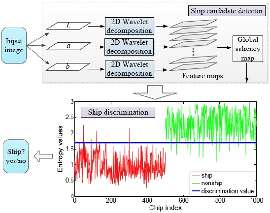
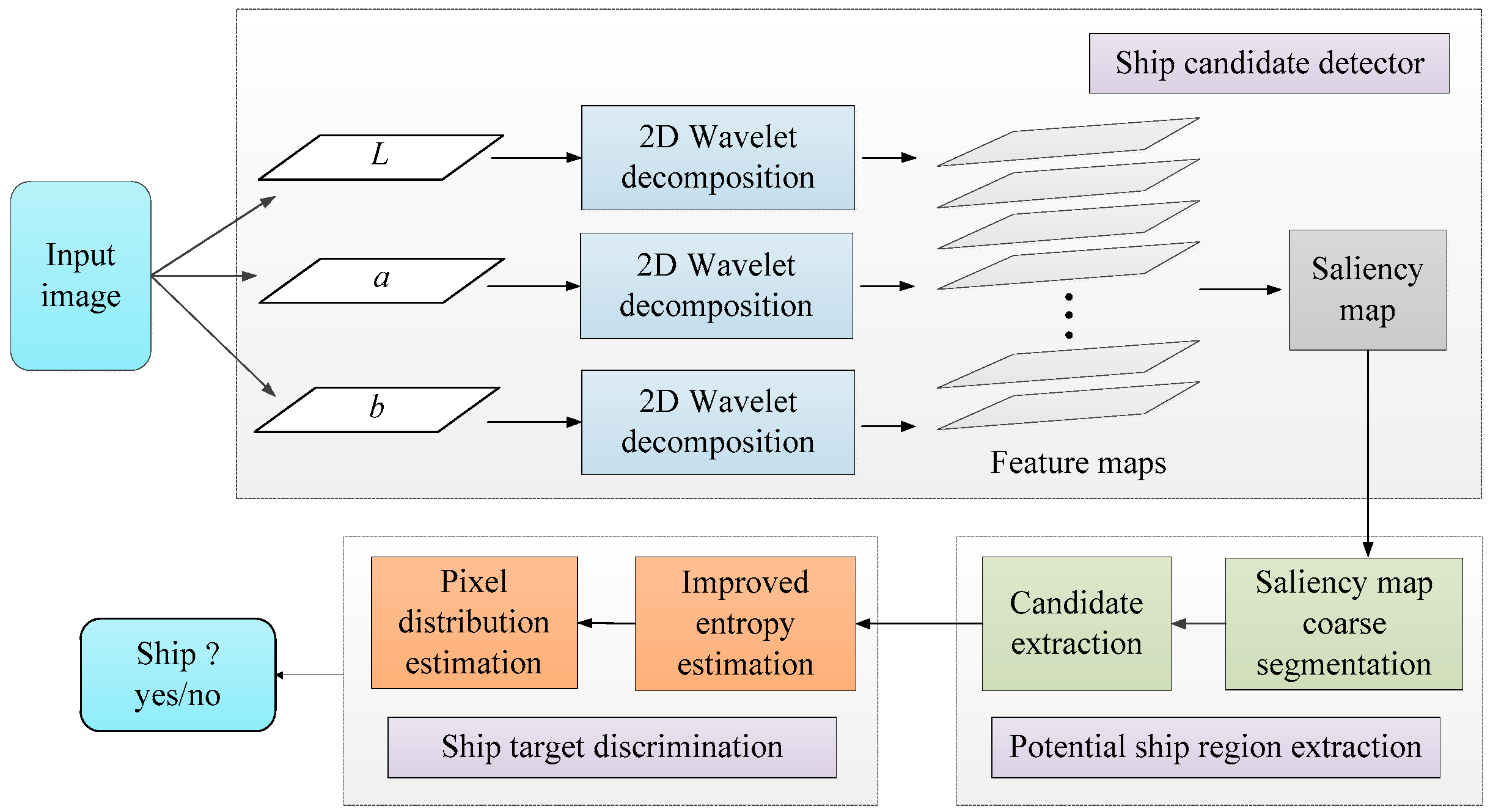
The overview of our detection approach is given in Figure 1, which covers the whole process from coarse to fine. First, ship candidates are extracted by saliency detection based on Wavelet transform. Some false alarms may be introduced including clouds, shadows, islands, and coastlines. Then, they are further removed in the discrimination stage, while the real ships are preserved.
2.2. Wavelet Decomposition
Wavelet transform (WT) is able to provide multi-scale spatial and frequency analysis at the same time. The multi-size filter banks are applied to process signals. For the input image, the approximate information and detailed information of the image can be obtained from the low-pass frequency bands and the high-pass frequency bands, respectively.
Ship targets are considered as the salient regions caused by the differences in colors, textures, shapes, and orientation factors. Wavelet coefficients can express them effectively based on the spatial-frequency analysis of the wavelet transform, which can examine the signal at different bands and bandwidths. Considering this fact, the factors including different colors, different scales, and different orientations are used for simulating our saliency model. Firstly, instead of using rgb color space in which the correlation of three color channels is quite large, the input image f(x,y)will be converted into the CIE Lab color space specified by the International Commission on Illumination. It is a color-opponent space including the lightness dimension L, and color-opponent dimensions a and b. All perceivable colors are included and its gamut exceeds rgb. Then, the sub-bands of each color channel will be generated by the multi-scale wavelet transform. Considering the filter size, computation time and detection effect, Daubechies wavelets (db.4) are chosen [35]. The multi-scale wavelet decomposition is defined as follows.
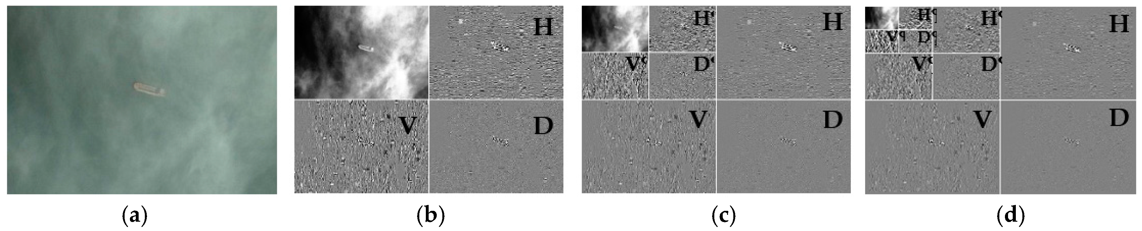
where (x,y) denotes the pixel index of the input image in the spatial domain, x∈[1,ro], y∈[1,co]. ro and co are the numbers of the row and column of the input image. c presents the color channel, and c ∈{L, a, b}. j is the decomposition level index, and j∈{1, …, J}. J is the maximum decomposition level and corresponds to the roughest resolution. For a N × N image, J = round[log2N], and round[·] means taking the integer part. WTj(·) is the jth level wavelet decomposition function. is the jth level scaling coefficient, which corresponds to the approximation output and represents the low-frequency information of each color channel in the image. The continuous decomposition for the low-frequency component of the input image is executed. , and denote the wavelet coefficients of horizontal, vertical and diagonal details for the different colors and decomposition levels, respectively. Some of the decomposition results are shown in Figure 2.
2.3. Feature Map Generation
The wavelet coefficients at the various levels can provide the details of the input image. A series of feature maps with the high-frequency data can be created by IWT operation, in which the approximation information is neglected. The feature maps are constructed as follows.
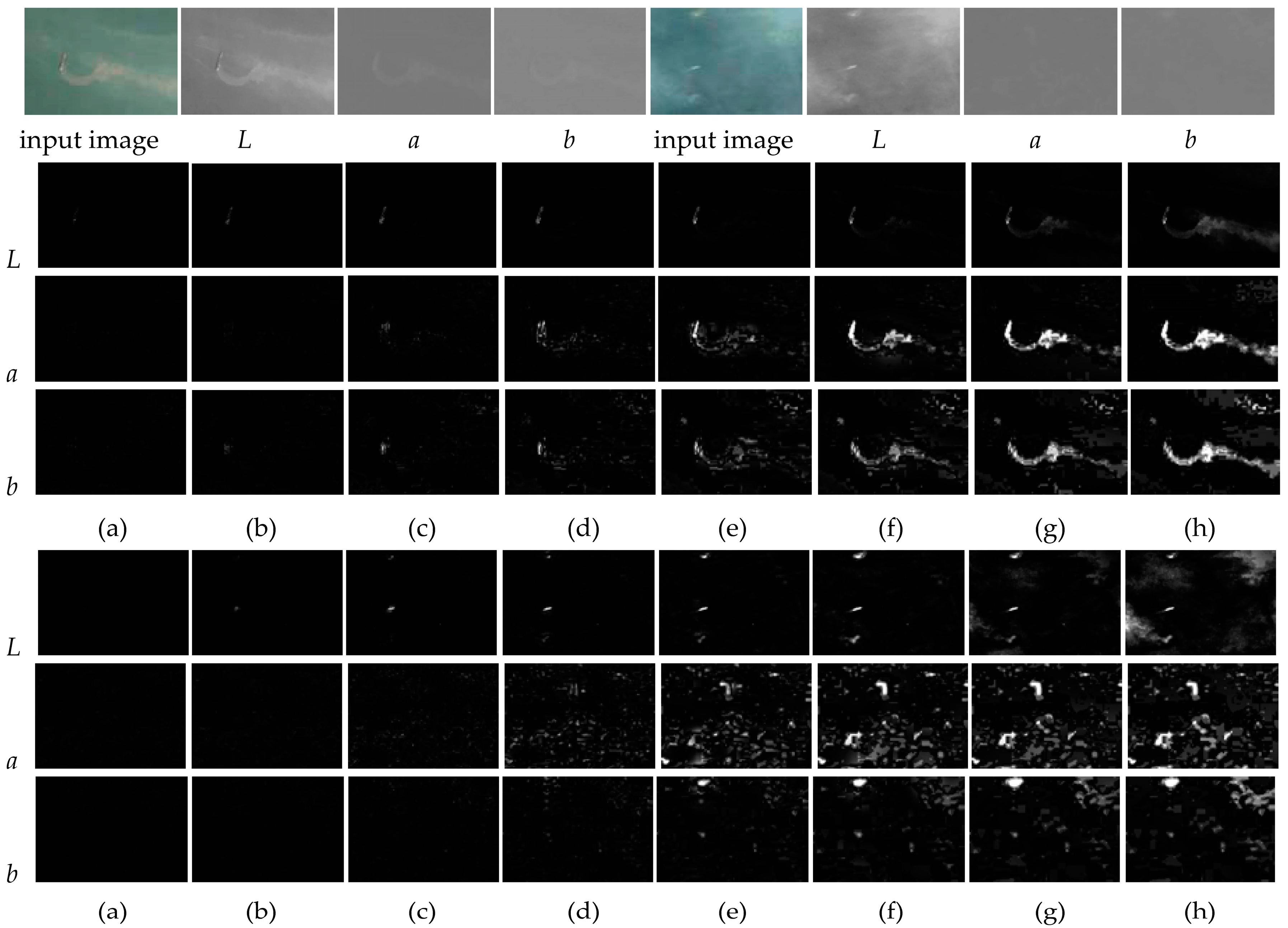
where fmjc(x,y) is the feature map constructed from the jth level in each color channel. IWTj(·) is the reconstruction function for , and by IWT without considering . The range of the feature values is relatively large in Equation (2). An appropriate p value is necessary, which can avoid the large variation in the calculation of the covariance matrix in Equation (4), and p is equal to 104 here after multiple experiments. There are two remote sensing images and their multi-level feature maps from the finest (1st) level to the coarsest (jth) level are shown in Figure 3. It is noted that the higher the level is, the more the interesting information is. The different detailed information of each decomposition level in the Lab color space is beneficial to the final saliency map.
2.4. Global Saliency Map Construction
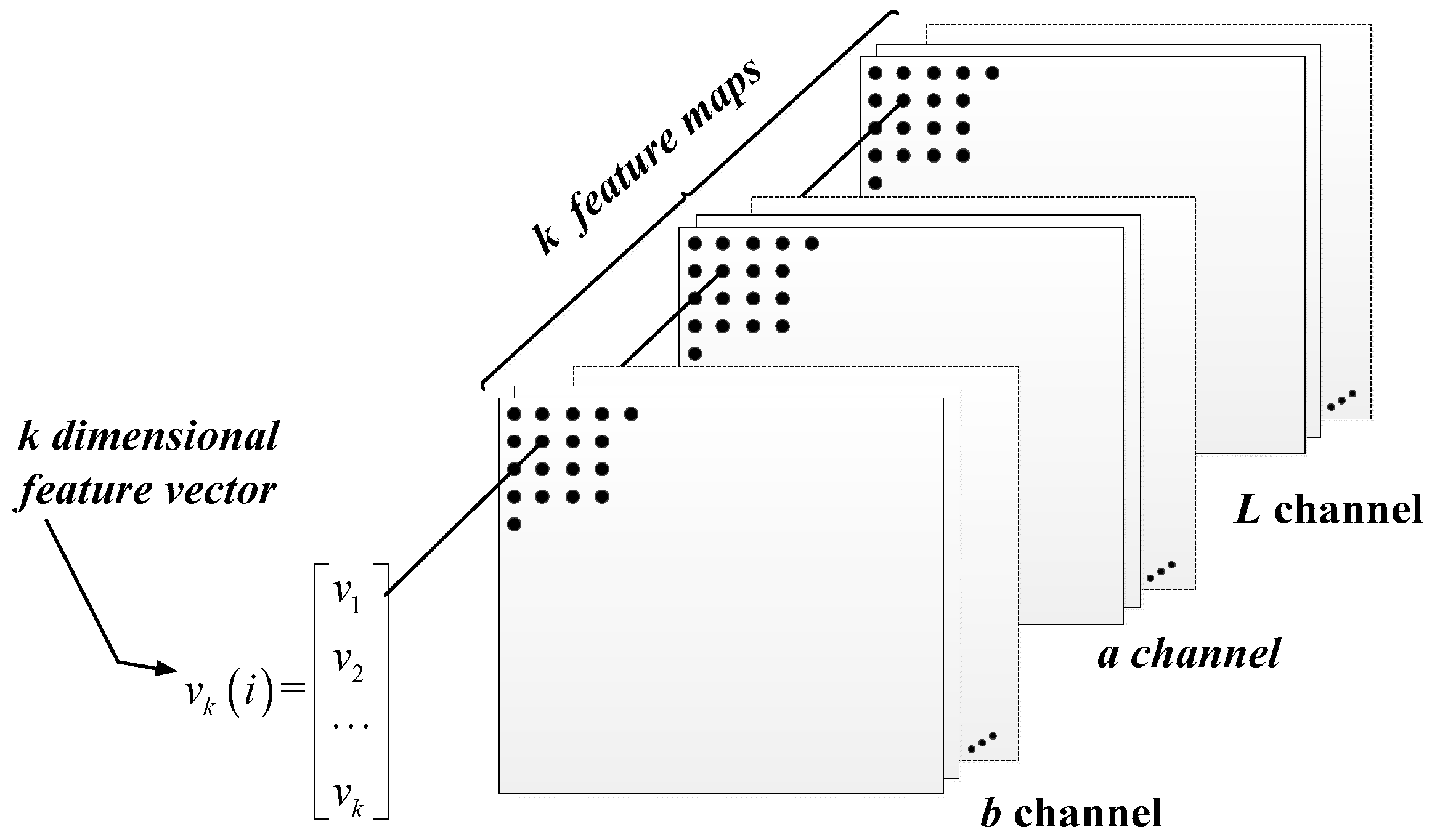
After obtaining 3 × J feature maps, the significance degree of each pixel position can be defined by the Gaussian probability density function. When the distribution probability of the position is small, its saliency is prominent. Otherwise, it is not salient. Inspired by this fact, the global saliency map is calculated as follows. The feature vector at the same pixel position among the feature maps can be defined as vk(i), i∈{1, …, ro × co }, and k = 3 × J. Multi-channel, multi-scale and multi-direction feature maps, and pixel by pixel feature vector are illustrated in Figure 4.
The multivariate Gaussian probability density at each pixel position is defined as follows.
where E[·] denotes the mathematical expectation operator. μ is the mean of the feature vector. C is the k × k dimensional covariance matrix and |C| is the determinant of the covariance matrix. T is the transpose operator.
The significance degree at each pixel position is inversely proportional to its probability [37,38], which can be computed as below.
Then, the global saliency map can be obtained as follows.
where G5×5 is a 5 × 5 2D Gaussian low-pass filter to get a better visual effect. The global saliency map S″(x,y) contains the statistical relation to all the feature maps and can highlight the important information that local contrast cannot detect. Figure 5 shows the hot maps of the global saliency maps by multi-level reconstruction. The more the high-frequency information of the saliency map is, the richer the information of interest is.
The brighter the color of the saliency map is, the more interesting the information is. We can see that the target region in the hot map is the most complete when the maximum level value is selected. Therefore, the global saliency map at the position of the coarsest decomposition level is retained, which can clearly describe the contour and shape structure of the ship.
2.5. Saliency Map Enhancement
In the saliency map S″(x,y), some interference information from the sea surface may be introduced. The distance decay formula is implemented to preserve the ship region and weaken the less significant regions. Considering that some ships in the sea background may be weak and small, differently from [24], we take the salient regions in S″(x,y) whose values are larger than 0.5 as the absolute saliency regions. (x″,y″) is the pixel index inside the region. The salient points (x,y) beyond the absolute saliency region are weighed by the minimum distance from these points to the absolute saliency region.
where S(x,y) is the final saliency map. dof(x,y) is the Euclidean distance from the salient point (x,y) to its nearest point (x″,y″), and dof’(x,y) is the normalized value of dof(x,y). The saliency values in S(x,y) around the absolute saliency region will remain unchanged or slightly decrease, while the salient values away from the absolute saliency region will largely decrease. Thus, the interference region can be removed effectively and the ship target with the high-frequency component can be highlighted.
3. Potential Ship Region Extraction
After the saliency detection, an adaptive segmentation based on the Otsu method [39] is executed to extract the potential ship target regions. The corresponding binary image can be obtained. After being multiplied with the input image, we define the connected regions covered by the bounding boxes as the ship candidates. To eliminate obvious false alarms, only the candidates of fewer than three thousand pixels and more than ten pixels in size are considered for further analysis. The numbers are related to the size of the input image and can be estimated in engineering application. After that, some target chips can be extracted. To ensure the integrity of the chip, each chip is extended by ten pixels along each dimension.
It is noted that the ships in the chips may be black or white polar, and appear as long symmetrical strip and their main axes are also randomly distributed. Some pseudo-targets, such as islands, coastlines, clouds, and shadows, may be included in the chips; therefore, each individual ship chip needs to be further verified as to whether the chip contains a real ship.
4. Target Discrimination
This stage is vital to the total detection results. However, the appearance of the ship is easily affected by the complex sea surface and the feature extraction for some small ships is hard. In addition, it is difficult for the current methods to juggle the distinguish accuracy and the computational complexity at the same time. To overcome these problems, a novel discrimination method is proposed based on the improved entropy estimation and pixel distribution for effectively eliminating the interferences according to the characteristics of the ship and no-ship chips.
4.1. Entropy Discrimination
Generally, the distributions of the chips with real ships are more regular, whereas the chips with pseudo targets are irregular. Inspired by this fact, we presented an improved entropy method for identifying the real ships. The entropy theory [40] is used for evaluating the random degree of the information distribution. Conventional entropy is based on the distribution of a variable e, defined as follows.
where pi denotes the histogram counts of an image. The index i is the grayscale, e∈[0,M], and the maximum M value is 255. When pi = 0, pilog(pi) = 0.
By definition, if the histogram of the pixel distribution of an image is given, its entropy value is determined. However, the spatial geometric information of the image is not considered in the conventional entropy definition, as shown in Figure 6.
In Figure 6, there are eight images with different context in total. Their resolutions are all 128 × 128. The numbers of the black and white pixels are equal and the distributions of the black and white pixel blocks are balanced. Although the distribution of the pixels is disordered, the histogram of the pixel distribution is same. They possess the same entropy value. Therefore, spatial geometric information needs to be considered for evaluating the random degree of the information distribution. We redefined a simple improved definition of the entropy for filling this gap. We achieve this purpose by considering each pixel of the image and the pixel values of its neighbors simultaneously. A Gaussian kernel is employed to filter the input image. Then, we calculate the entropy value of the filtered image, the definition of the improved entropy is written as follows.
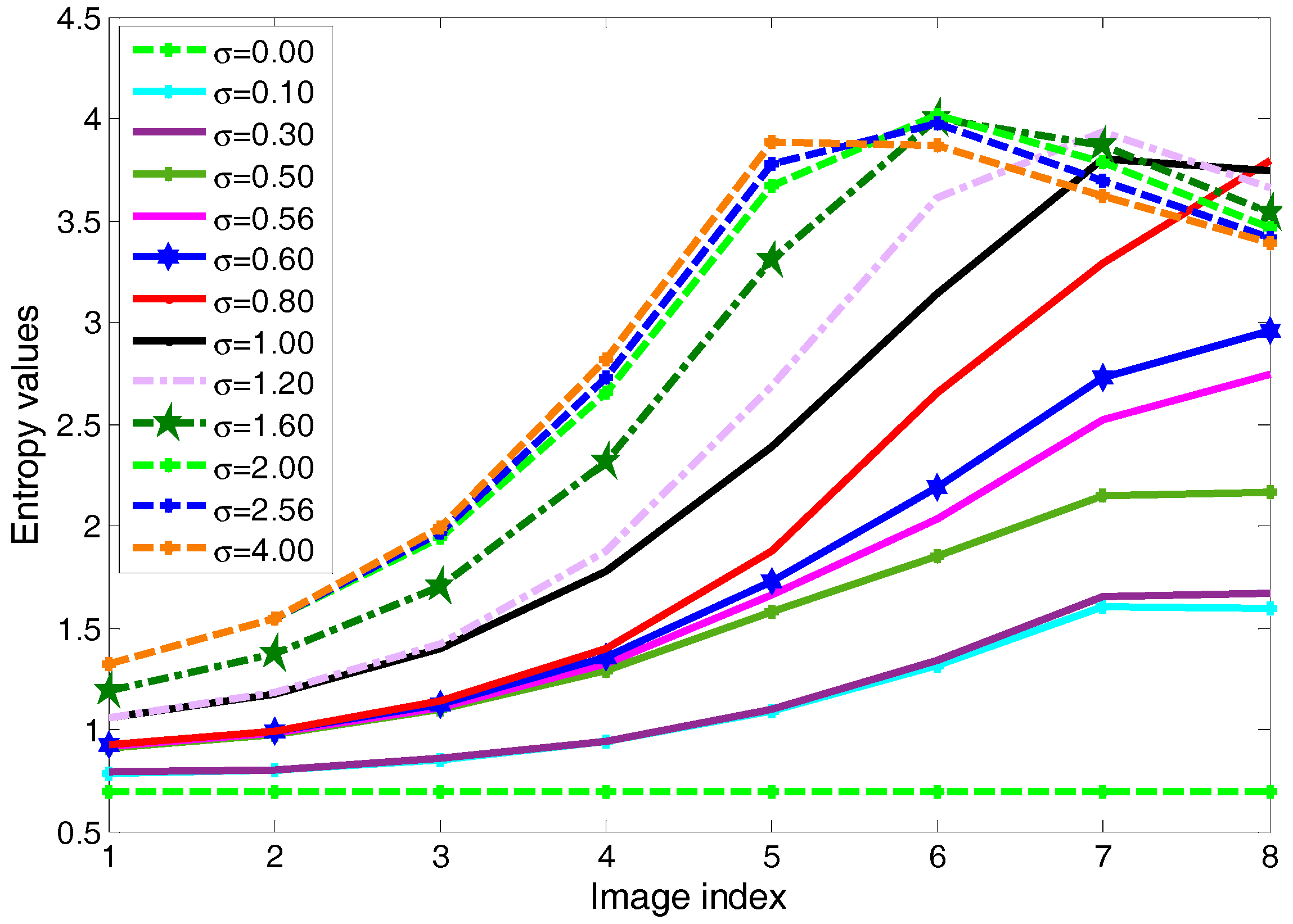
where g is a two-dimensional low-pass Gaussian filter. σ is the standard deviation of Gaussian kernel. Fix the template size of the filter, and we change the σ value. The entropy values of the eight images in Figure 6 can be calculated, as shown in Figure 7.
As we can see in Figure 7, the entropy values of the eight images are equal when σ = 0; the Gaussian filter has almost no effect on the input image. If σ is relatively small, the Gaussian filter has a minor effect on the input image. The entropy values gradually increase. If σ is particularly large, the entropy may first increase and then decrease. That is because the Gaussian filter destroys some small structures of the input image. Experiments indicate that σ∈(0.1,1.0) can yield acceptable results. Considering the monotonicity of the entropy variation, the size and the pixel distribution of the chip, σ = 0.56 is selected.
The distribution of the target pixels in the chips can be considered as a probability map. For the chip containing a real ship, the ship target appears as a long symmetrical strip and its pixel distribution is relatively centralized. The texture distribution of the chip is regular. Otherwise, the distribution is disordered. After many experiments, according to the new definition of the entropy, the entropy value of the chip containing a ship is generally small. The entropy value increases when a pseudo-target exists. Therefore, the improved entropy value is employed as the criterion for discriminating the ship and non-ship targets.
The input chips are converted into the binary images by an adaptive segmentation based on the Otsu method, and their entropy values are subsequently calculated. The entropy results from different chips are presented in Figure 8. The chips come from the saliency detection and manual extraction. The former 500 chips are the ship chips and the latter 500 chips contain the pseudo targets.
As we can see, the ship and non-ship targets can be discriminated by this improved entropy estimation. The blue line denotes the discrimination threshold of the ship and non-ship targets, and is indicated as T, which is critical for the discrimination accuracy. Let the entropy values of the chips with the ships be Sn, while those of the false alarms are Fn. n denotes the number index of the chips. The ideal threshold T* can be calculated as follows.
where Ta is the mean of the average entropy values of the ship and non-ship targets. CS(·) counts the total amount that satisfies the conditions in the brackets. If the entropy value of the binary chip is less than T*, the chip contains the real ship. Otherwise, it is not a real ship and is removed. Using this discrimination principle, there is no need to build a large number of samples in advance, finely segment the chip, and extract the specific features of the target.
4.2. Pixel Distribution Discrimination
According to the entropy discriminative condition, if the entropy value of the chip falls below the threshold, the target is viewed as a real ship, otherwise not. In Figure 8, it is noted that the entropy values of four ships described by red line are above T*, and mistaken as non-ship targets. The complex scenes lead to the missed detection. The entropy values of 14 pseudo targets represented by green line are below T* and identified as the ship targets, which are viewed as the false alarms.
After numerous experiments, it is noted that the entropy values of the false chips may be confused as those of the ship chips when the following cases occur. (1) There are very few target pixels in the chips. (2) The chips contain clouds, shadows, and coastlines. After binarization, the target pixels in these chips may distribute along one edge or the two adjacent edges. (3) Some small bright islands or heavy clouds are inside the chips. Some illustrations are shown in Figure 9.
To solve the problems discussed above, a new discrimination method based on the pixel distribution is designed for further eliminating these pseudo targets. In the binary chip with real ship target, the ship mainly distributes inside the chip and the pixel area of the ship region is smaller than that of the whole chip. The pixels on the four edges of the chip are almost the background. Based on this, we can determine whether the target pixels of the chip are black or white. Firstly, the number of black and white pixels on four edges is counted. If there are none of these pixels on the four edges of the chip, or their number is less than the half of the total number of the pixels on the four edges, they can be viewed as the target pixels. After that, we can remove the non-ship chips according to the following ten judgment conditions, which are indicated by ➀➁➂➃➄➅➆➇➈➉, as shown in Figure 10.
In Figure 10, the blue parts are the four edges of the chip, and the gray one is the target to be identified. The specific discrimination principles are listed as follows. (1) If the number of the target pixels in the chip is less than five ➀, the chip contains the non-ship target and needs to be removed. The threshold size can be estimated by the resolution of the input image. (2) Along the four edges of the chip, if the target pixels distribute on at least one edge and their number is greater than 75% of the total number of the pixels on the entire edge ➁➂➃➄, the chip contains the non-ship target. In addition, if the target pixels distribute on the two adjacent edges and their number is greater than 65% of the total number of the pixels on the two edges ➅➆➇➈, they are also identified as non-ship targets and removed. (3) If the target is inside the chip, and the pixel area of the target is greater than 22% of the total pixel area of the chip ➉, the chip contains the pseudo target and needs to be removed. After the process above, the number of the false alarms can further decrease. Moreover, the calculation speed is very fast.
5. Experimental Results and Discussion
To validate the performance of our method, multiple tests are implemented from both subjective and objective aspects. The remote sensing images from the publicly available Google Earth service are used to perform the experiments. They are randomly selected from the eastern coast of China. In total, 273 representative images with the resolution of 2–15 m cover plenty of scenarios and the size of each test image is 300 × 210 pixels. The ship targets that may be black or white polar are under a variety of sea backgrounds, such as heavy clouds, shadows, ship wakes, coastlines, small islands and reefs. In addition, the pixel sizes of the ship targets vary from seven to hundreds.
5.1. Subjective Visual Evaluation of Saliency Models
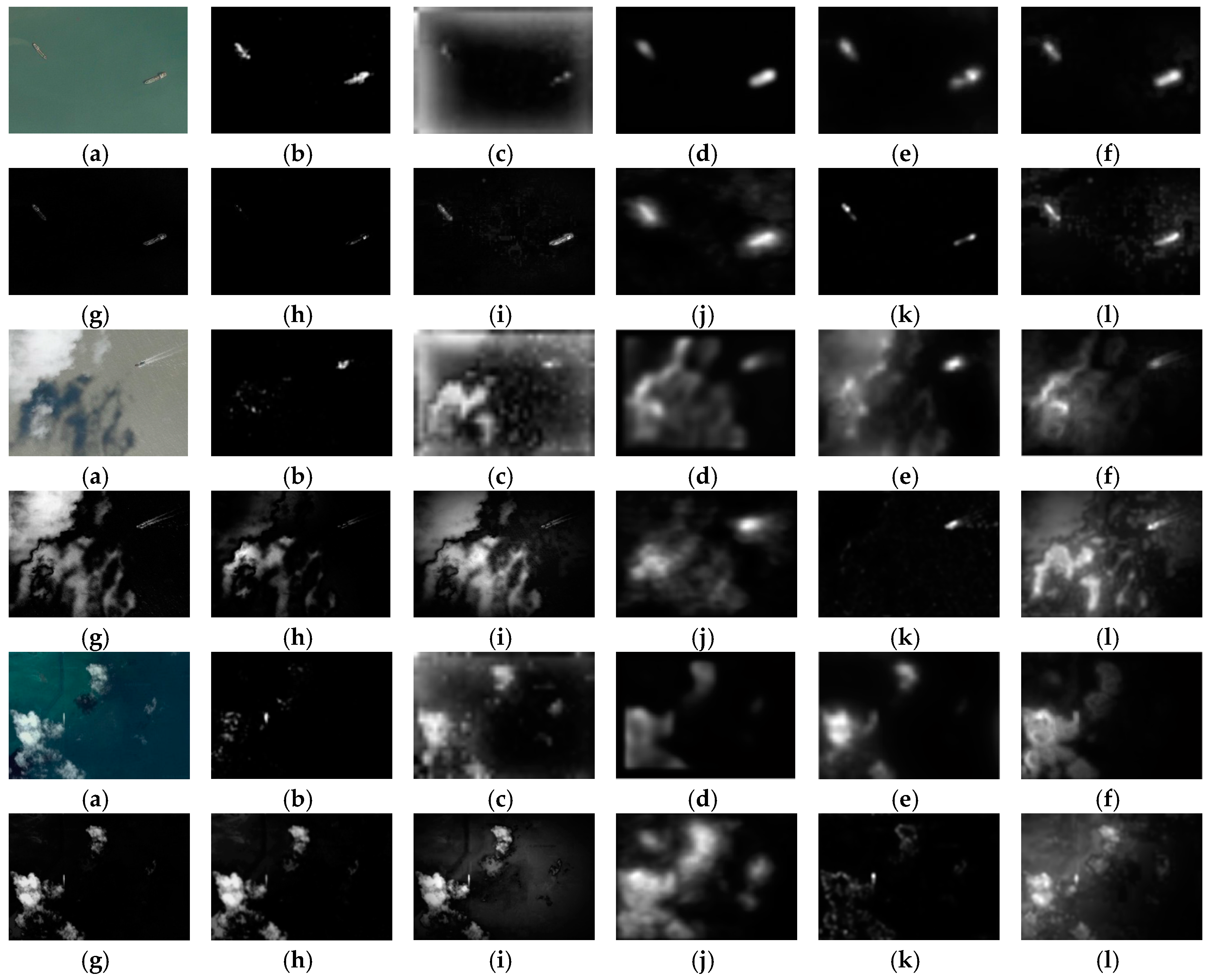
Figure 11 and Figure 12 illustrate some comparisons with our saliency model against other typical models including the spatial, Fourier transform, and Wavelet transform domains in subjective visual representation. There are eight groups in total and each group has 12 images, including the input image, the results of our saliency model (WGS) and ten other models. The saliency model [35] in wavelet domain is called Nevrez for short.
Figure 11 displays the comparisons from the background suppression and target highlighting abilities of the different models. Some input images have simple and calm sea backgrounds. The ships may be different sizes and colors. Contrarily, other images are under complex sea conditions including thin clouds, heavy clouds, shadows, and ship wakes.
In Figure 11, it is noted that the detection performance of the WGS model is better and has successfully suppressed the undesired sea backgrounds and highlighted all the real ship targets. Although the ITTI, AIM, GBVS, CA, and RARE models can find the ship target locations, their background suppression abilities are weak. A lot of interference information is involved in their saliency maps, which may affect the subsequent processing speed and accuracy. Although the detection results are finer for the LC, MSSS and SDSP models, some ship targets may be missed in some cases caused by heavy clouds and dark ships, as shown in the first three groups. The detection results show that the SR model is effective for the images with clouds and mist, and most of the sea backgrounds are suppressed. However, it can only deal with gray images. The integrity of the ship target is poor and the whole ship region may be segmented into some small pieces as shown in the first and second groups. Although the Nevrez model is also based on the wavelet domain, the saliency detection results are relatively poor since the maximum value among the different color channels is considered at each level and the final saliency map is dominated by the local saliency. Compared with the other models, WGS can suppress many sea surface interferences including clouds and shadows. Although some ships are dark and they have much lower intensity than the sea surface background, WGS has successfully highlighted them and the integrities of the ship regions are well maintained.
Figure 12 shows the saliency detection results of the eleven saliency models on the input images with the reefs, coastlines and islands.
After a general comparison among the eleven saliency models, we can find that the ship target can be well highlighted by all the models when the coastlines and islands are dim. However, compared with the WGS model, a large amount of false alarms are also highlighted in the other ten models, as shown in the first three groups. In the fourth group of the images with the bright island, the capability of detecting ship targets from the ten models is greatly weakened. The island is highlighted, while the ship region detected is dim and weak. Several ships are even missed in some models. Although the background suppression ability of the SR model is stronger than the other nine models, the detection result is still poor when the coastline has a bright edge or the island exists with the bright background, and the ship targets may be missed. Compared with the other ten models, the WGS model can achieve better detection results. The ship targets under the various complex sea backgrounds can be detected accurately and stably. The shape and the structure information of the ship targets are better maintained. Although some scattered interferences may still be introduced, the pseudo target can be largely eliminated in the subsequent ship target identification. In addition, it is conducive to the discrimination process, and the computational speed can be greatly improved because of the low repetition and the smaller amounts of false alarms.
5.2. Objective Quantitative Analysis
To evaluate the performance of different saliency models objectively and quantitatively, this section validates the eleven saliency models from the saliency detection precision and calculation speed. In addition, the capability of the saliency models on the images with different pixel sizes is also tested and analyzed.
To evaluate the integrity and precision of the ship target region detected by the saliency models, the Receiver Operating Characteristic (ROC) curve is computed, which plots the True Positive Rate (TPR) against the False Positive Rate (FPR). First, for the remote sensing image in the image database, we manually mark its ground-truth map G as the criterions of evaluations and analysis. The ground-truth map G refers to the accurate hull of the ship region in the input image, which is a binary map, and considered as prior information. Figure 13 shows the ground-truth maps of some test images.
Then, a series of fixed integers from 0 to 255 are used as the threshold of the saliency map detected to obtain 256 binary images S. S is compared with the corresponding G, then, the four parameters can be counted as follows. The pixels belonging to G and S simultaneously are called True Positive (TP). The pixels belonging to G and not belonging to S are called False Negative (FN). The pixels not belonging to G and belonging to S are called False Positive (FP). The pixels not belonging to G and S simultaneously are called True Negative (TN). A set of TPR and FPR can be defined as follows.
For each saliency model at the threshold, there are 256 average TPR values and 256 average TPR values in total. The ROC curves can be plotted, as shown in Figure 14a. The Area Under the Curve (AUC) of each model is also calculated, as shown in Figure 14b.
If the curve is closer to the upper left corner, the performance of the saliency model is better. We can see the ROC curve of the WGS model is higher than those of the tenother models. For a more intuitive comparison, the closer the AUC value of the model is to 1, the better the saliency detection performance is. As we can see in Figure 14b, the AUC value of the WGS model is the largest and it consistently outperforms the other ten models.
The time cost is compared among the WGS model and the ten other state-of-the-art models. All experiments in this paper are conducted using a PC with an Intel Core 3.30 GHz processor and 4 GB of RAM. The programming platform is built in Matlab 2014a and called M for short. The time consumption of each model is shown in Table 1.
In Table 1, the average computing time of LC is the shortest because of the simple calculation. Compared with the processing speed of AIM, GBVS, CA and Nevrez, WGS is more time-efficient, while it is slower than the other six models. The main reason that affects its running speed lies in the calculation of the global saliency map using the probability density function on the multiple feature maps. This process is a time-consuming operation and consumes 1.204 s. While the time cost of the feature map generation using IWT is 0.829 s.
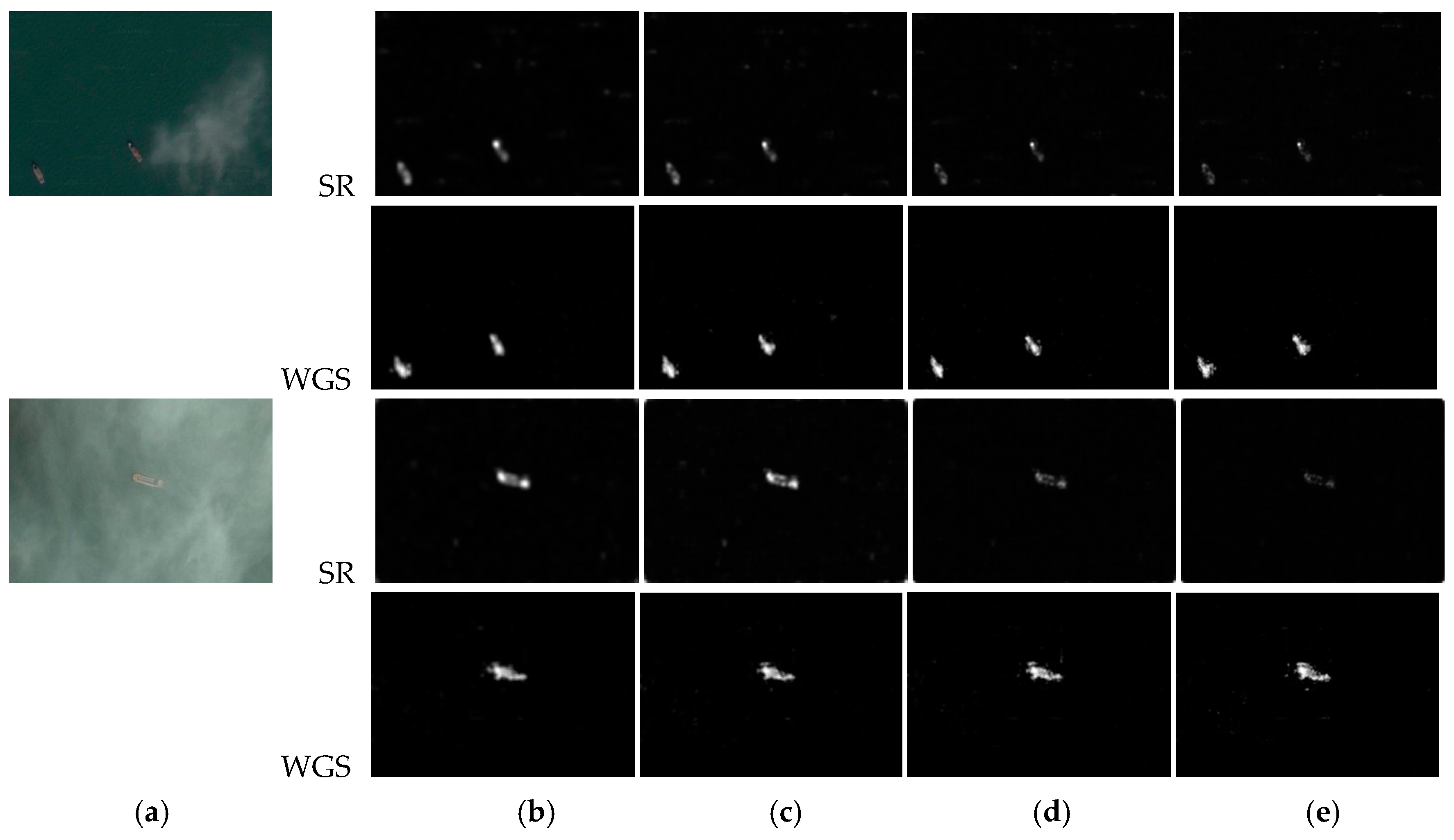
In addition, we test the capability of the saliency models on the images with different pixel sizes. Most saliency models are constructed using the low-level features of the input images, which are sensitive to the image size. The results of saliency detection on the images with different sizes may vary greatly. Therefore, we make a test on the multi-size images. In terms of detection performance in Figure 11 and Figure 12, SR is selected for comparing with WGS. The pixel sizes of the input images are 300 × 210, 406 × 283, 505 × 354, and 612 × 428. The detection results by the SR and WGS models are shown as follows.
As we can see in the two sets of results from Figure 15, with the increase of the input image size, the information of interest is less and the integrity of target regions gradually decreases in the SR model. The saliency detection performance of SR becomes worse. Compared with SR, the detection effect of WGS for the images with different sizes is better owing to the characteristics of the multi-scale and multi-direction wavelet analysis. In the saliency maps of WGS, the background interferences can be suppressed effectively and the ships can be extracted accurately with a good integrity.
5.3. Overall Result Statistics
To evaluate the overall effectiveness of the ship extraction and each discrimination stage, the constructed image database includes plenty of images with islands, coastlines, reefs, heavy clouds and shadows, in addition to the simple and calm sea backgrounds. The detection accuracy ratio (Cr), missing ratio (Mr) and false alarm ratio (Far) are computed, which are defined as follows.
where Nt is the total number of the real ships in the database. Ntt is the number of correctly detected ships. Nfa is the number of the false alarms. The detailed extraction and discrimination results after each stage are presented in Table 2, which gives some reflections on the detection performance of the whole algorithm in each phase listed as follows. We only execute the global saliency detection based on the wavelet transform (abbreviated as WGS). The false alarms are preliminarily identified according to the sizes of the chips (abbreviated as SCD). The discrimination is based on the improved entropy (abbreviated as IED). The discrimination is executed based on the pixel distribution (abbreviated as PDD).
As we can see in the first row of the table, a few ships may be missed when only using the WGS model. That is because the details of the faint and small ships are not obvious when multiple ships with different sizes and colors exist. Their information may be ignored when the high-frequency wavelet coefficients are calculated for constructing the saliency map. In addition, the distance decay process will further weaken the significance level of the small ship targets and lead to the missed detection. We also find that the number of the false alarms is great in this stage. That is because there are many scattered false alarms in the saliency maps when the strong interferences exist, such as the islands and coastlines with the complex distribution, heavy clouds and shadows. After the adaptive threshold segmentation using the Otsu method, dozens of false alarms may be introduced in an image. Although some false alarms can be reduced by increasing the threshold in the segmentation, the ship pixel area of the chip may also decrease. It may result in the missed detection in the SCD stage. Therefore, it is safely concluded the saliency detection results using wavelet transform are accepted on the sea background without bright coastlines and islands. No false alarms or a small amount of false alarms is introduced in this case. Otherwise, plenty of the false alarms under the complex backgrounds may be introduced after binarization. In the second row of the table, although Cr has gone down by 0.898% after the SCD stage, Far decreases by 5.041%. In the third row of the table, a few real ships are identified as the false alarms under some complex backgrounds and Cr drops by 4.668% after implementing the IED stage. However, Far has reduced by 25.635%, which shows the effectiveness of the discrimination stage based on the improved entropy estimation. At last, for the false alarms whose entropy values are similar to those of the ships, we design the PDD stage for further removing them. After that, Far decreases to 5.741%. In addition, the chips containing the smaller targets can be effectively removed and this discrimination stage can achieve high detection adaptability and robustness. Through the analysis above, it is safely concluded that the multi-level false alarm discrimination method is effective for eliminating the pseudo targets and retaining the real ships. The detection performance of the whole method is improved greatly after these stages.
With regard to the computation time of the whole discrimination stage, it depends on the number and sizes of the chips. The more the candidates in the input image are, and the larger the chip size is, the higher the time consumption becomes. For the target chips with different sizes 17 × 18, 51 × 30 and 64 × 64, the average running time of each auxiliary algorithm including SCD, IED and PDD is shown in Table 3, respectively. We can see the computation speed of each stage is very fast and a desirable time performance can be achieved.
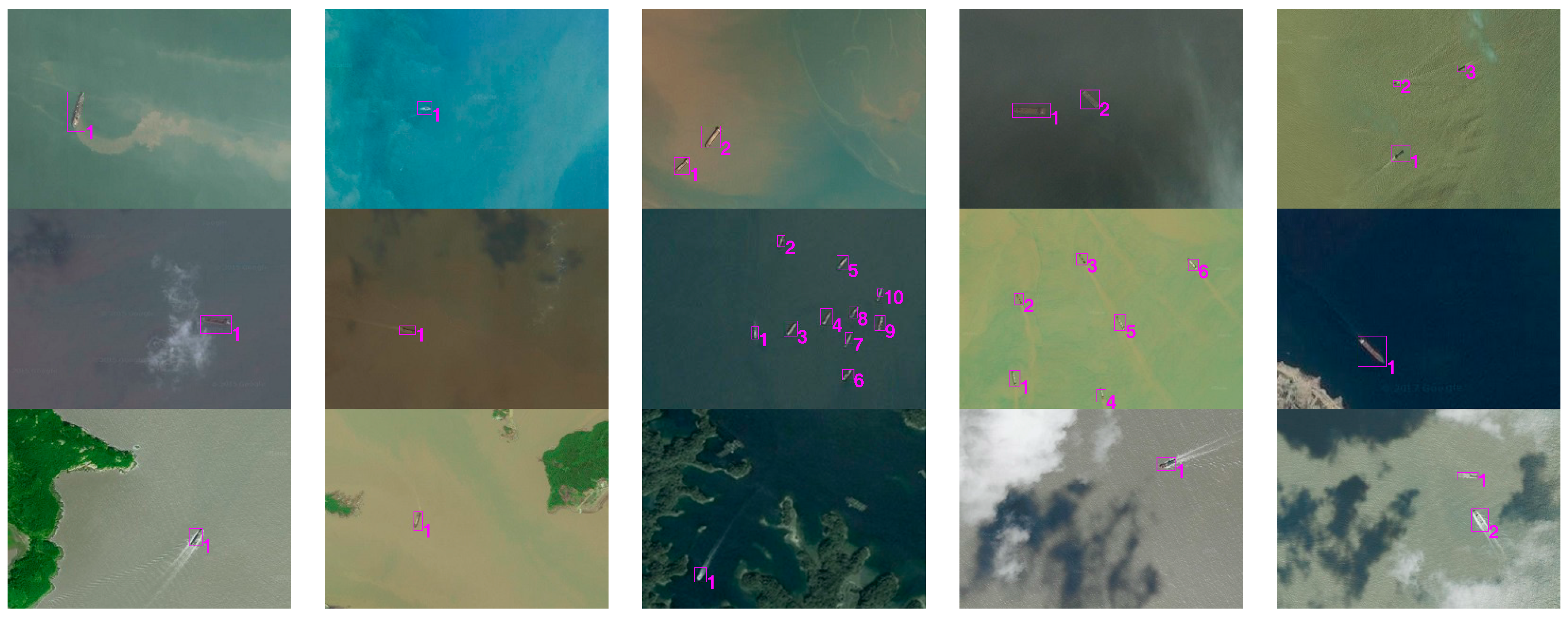
Some typical detection results for color images are displayed in Figure 16. We can see most false alarms are eliminated, whereas the real ship targets are extracted after the multi-level discrimination. The regions containing real ships are detected and marked with the pink boxes. It is noted that the number and the locations of ships are determined accurately.
6. Conclusions
In this paper, a novel detection framework consisting of saliency detection and discrimination stages is presented for detecting and extracting ship targets from optical remote sensing images. To extract the ship candidates against the complex sea backgrounds, a global saliency model is constructed based on the multi-scale and multi-direction high-frequency wavelet coefficients. Then, the distance decay formula is implemented to weaken the non-salient information in the saliency map. The large range low-frequency information from the sea background can be suppressed, while most ship regions with clearer contours can be extracted accurately. The ship regions extracted are uniform and complete. In addition, the images with different sizes can be effectively processed by the proposed saliency model. Furthermore, to eliminate the islands, coastlines, heavy clouds, shadows and small clutter regions, a multi-level discrimination method is designed. According to the characteristics of the ship and no-ship chips, the improved entropy estimation is presented, which overcomes the deficiency of the traditional entropy relying on spatial geometric information. It can remove the false candidates and retain the real ship targets. For the false chips whose entropy values are confused with those of the ship targets, the pixel distribution identification is proposed to further decrease the false alarm rate. Experimental results on the images under various sea backgrounds demonstrate that the proposed method can achieve high detection robustness and a desirable speed performance.
Although our method has achieved promising results, several issues remain to be further settled and improved. In the discrimination stage, a few candidates may contain the slender reefs similar to the shape of the ship or the coastline with the bright edges. After binarization, their entropy values are similar to those of the ship chips, and they are difficult to be removed. More effective features and further attempts should be made to remove such false alarms.
Acknowledgments
We acknowledge the financial support that was given under the Project supported by the National Defense Pre-Research Foundation of China (Grant No. 402040203). This study was also supported by the Programs Foundation of Key Laboratory of Airborne Optical Imaging and Measurement, Chinese Academy of Sciences (Grant No. y3hc1sr141). We acknowledge associate editors and anonymous reviewers for their constructive comments and suggestions.
Author Contributions
Fang Xu and Jinghong Liu provided the detection idea. Fang Xu, and Chao Dong designed the experiments. Jinghong Liu, Fang Xu and Xuan Wang analyzed the experiments. Fang Xu and Chao Dong wrote the paper together.
Conflicts of Interest
The authors declare no conflict of interest.
References
- Velotto, D.; Bentes, C.; Tings, B.; Lehner, S. First comparison of Sentinel-1 and TerraSAR-X data in the framework of maritime targets detection: south Italy case. IEEE J. Ocean. Eng. 2016, 41, 993–1006. [Google Scholar]
- Brusch, S.; Lehner, S.; Fritz, T.; Soccorsi, M.; Soloviev, A.; Schie, B.V. Ship surveillance with TerraSAR-X. IEEE Trans. Geosci. Remote Sens. 2011, 49, 1092–1101. [Google Scholar] [CrossRef]
- Schwegmann, C.P.; Kleynhans, W.; Salmon, B.P. Synthetic aperture radar ship detection using Haar-like features. IEEE Trans. Geosci. Remote Sens. Lett. 2017, 14, 154–158. [Google Scholar]
- Proia, N.; Pagé, V. Characterization of a Bayesian ship detection method in optical satellite images. IEEE Trans. Geosci. Remote Sens. 2010, 7, 226–230. [Google Scholar] [CrossRef]
- Corbane, C.; Najman, L.; Pecoul, E.; Demagistri, L.; Petit, M. A complete processing chain for ship detection using optical satellite imagery. Int. J. Remote Sens. 2010, 31, 5837–5854. [Google Scholar]
- Xu, Q.Z.; Li, B.; He, Z.F.; Ma, C. Multiscale contour extraction using level set method in optical satellite images. IEEE Trans. Geosci. Remote Sens. Lett. 2011, 8, 854–858. [Google Scholar]
- Yang, G.; Li, B.; Ji, S.F.; Gao, F.; Xu, Q.Z. Ship detection from optical satellite images based on sea surface analysis. IEEE Trans. Geosci. Remote Sens. 2014, 11, 641–645. [Google Scholar]
- Sun, H.; Sun, X.; Wang, H.Q.; Li, Y.; Li, X.J. Automatic target detection in high-resolution remote sensing images using spatial sparse coding bag-of-words models. IEEE Trans. Geosci. Remote Sens. Lett. 2012, 9, 109–113. [Google Scholar]
- Cheng, G.; Han, J.W.; Zhou, P.C.; Guo, L. Multi-class geospatial object detection and geosgraphic image classification based on collection of part detectors. ISPRS J. Photogramm. Remote Sens. 2014, 98, 119–132. [Google Scholar]
- Cheng, G.; Han, J.W.; Guo, L.; Qian, X.L.; Zhou, P.C.; Yao, X.W.; Hu, X.T. Object detection in remote sensing imagery using a discriminatively trained mixture model. ISPRS J. Photogramm. Remote Sens. 2013, 85, 32–43. [Google Scholar]
- Cheng, G.; Han, J.W. A survey on object detection in optical remote sensing images. ISPRS J. Photogramm. Remote Sens. 2016, 117, 11–28. [Google Scholar] [CrossRef]
- Yokoya, N.; Iwasaki, A. Object detection based on sparse representation and Hough voting foroptical remote sensing imagery. IEEE J. Sel. Top. Appl. Obs. Remote Sens. 2015, 8, 2053–2062. [Google Scholar] [CrossRef]
- Wang, X.; Shen, S.Q.; Ning, C.; Huang, F.C.; Gao, H.M. Multi-class remote sensing object recognition based on discriminative sparse representation. Appl. Opt. 2016, 55, 1381–1394. [Google Scholar] [CrossRef] [PubMed]
- Zhu, C.R.; Zhou, H.; Wang, R.S.; Guo, J. A novel hierarchical method of ship detection from spaceborne optical image based on shape and texture features. IEEE Trans. Geosci. Remote Sens. 2010, 48, 3446–3456. [Google Scholar] [CrossRef]
- Shi, Z.W.; Yu, X.R.; Jiang, Z.G.; Li, B. Ship detection in high-resolution optical imagery based on anomaly detector and local shape feature. IEEE Trans. Geosci. Remote Sens. 2014, 52, 4511–4523. [Google Scholar]
- Tang, J.X.; Deng, C.W.; Huang, G.B.; Zhao, B.J. Compressed-domain ship detection on spaceborne optical image using deep neural network and extreme learning machine. IEEE Trans. Geosci. Remote Sens. 2015, 53, 1174–1185. [Google Scholar] [CrossRef]
- Zou, Z.X.; Shi, Z.W. Ship detection in spaceborne optical image with SVD networks. IEEE Trans. Geosci. Remote Sens. 2016, 54, 5832–5845. [Google Scholar] [CrossRef]
- Yu, Y.; Yang, J. Visual Saliency Using Binary Spectrum of Walsh–Hadamard Transform and Its Applications to Ship Detection in Multispectral Imagery. Neural Proc. Lett. 2017, 45, 759–776. [Google Scholar] [CrossRef]
- Bi, F.K.; Zhu, B.C.; Gao, L.N.; Bian, M. A visual search inspired computational model for ship detection in optical satellite images. IEEE Trans. Geosci. Remote Sens. Lett. 2012, 9, 749–753. [Google Scholar]
- Zhu, J.; Qiu, Y.; Zhang, R.; Huang, J.; Zhang, W. Top-down saliency detection via contextual pooling. J. Signal Process. Syst. 2014, 74, 33–46. [Google Scholar] [CrossRef]
- Itti, L.; Koch, C.; Niebur, E. A model of saliency-based visual attention for rapid scene analysis. IEEE Trans. Pattern Anal. Mach. Intell. 1998, 20, 1254–1259. [Google Scholar]
- Bruce, N.D.; Tsotsos, J.K. Saliency based on information maximization. Adv. Neural Inf. Process. Syst. 2006, 18, 155–162. [Google Scholar]
- Harel, J.; Koch, C.; Perona, P. Graph-based visual saliency. Adv. Neural Inf. Process. Syst. 2006, 19, 545–552. [Google Scholar]
- Stas, G.; Lihi, Z.M.; Ayellet, T. Context-aware saliency detection. IEEE Trans. Pattern Anal. Mach. Intell. 2012, 34, 1915–1926. [Google Scholar]
- Zhai, Y.; Shah, M. Visual attention detection in video sequences using spatiotemporal cues. In Proceedings of the 14th ACM International Conference on Multimedia, Santa Barbara, CA, USA, 23–27 October 2006. [Google Scholar]
- Achanta, R.; Süsstrunk, S. Saliency detection using maximum symmetric surround. In Proceedings of the International Conference on Image Processing, Hong Kong, China, 1–4 September 2010. [Google Scholar]
- Riche, N.; Mancas, M.; Duvinage, M.; Dutoit, T. RARE2012: A multi-scale rarity-based saliency detection with its comparative statistical analysis. Signal Proc. Image Commun. 2013, 28, 642–658. [Google Scholar] [CrossRef]
- Zhang, L.; Gu, Z.Y.; Li, H.Y. SDSP: A novel saliency detection method by combining simple priors. In Proceedings of the IEEE International Coference on Image Processing, Melbourne, Australia, 15–18 September 2013. [Google Scholar]
- Hou, X.D.; Zhang, L. Saliency detection: A spectral residual approach. In Proceedings of the IEEE Conference on Computer Vision and Pattern Recognition, Minneapolis, MN, USA, 17–22 June 2007. [Google Scholar]
- Guo, C.L.; Ma, Q.; Zhang, L.M. Spatio-temporal saliency detection using phase spectrum of quaternion Fourier transform. In Proceedings of the 2008 IEEE Conference on Computer Vision and Pattern Recognition, Anchorage, AL, USA, 23–28 June 2008. [Google Scholar]
- Ding, Z.H.; Yu, Y.; Wang, B.; Zhang, L.M. An approach for visual attention based on biquaternion and its application for ship detection in multispectral imagery. Neurocomputing 2012, 76, 9–17. [Google Scholar] [CrossRef]
- Li, J.; Levine, M.D.; An, X.J.; Xu, X.; He, H.G. Visual saliency based on scale-space analysis in the frequency domain. IEEE Trans. Pattern Anal. Mach. Intell. 2012, 35, 1–16. [Google Scholar] [CrossRef] [PubMed]
- Ma, X.L.; Xie, X.D.; Lam, K.M.; Zhong, Y.S. Efficient saliency analysis based on wavelet transform and entropy theory. J. Vis. Commun. Image R. 2015, 30, 201–207. [Google Scholar] [CrossRef]
- Murray, N.; Vanrell, M.; Otazu, X.; Parraga, C.A. Saliency estimation using a non-parametric low-level vision model. In Proceedings of the IEEE Conference on Computer Vision and Pattern Recognition (CVPR), Colorado Springs, CO, USA, 20–25 June 2011. [Google Scholar]
- İmamoğlu, N.; Lin, W.S.; Fang, Y.M. A saliency detection model using low-level features based on wavelet transform. IEEE Trans. Multimed. 2013, 15, 96–105. [Google Scholar] [CrossRef]
- Xu, F.; Liu, J.H.; Sun, M.C.; Zeng, D.D.; Wang, X. A Hierarchical Maritime Target Detection Method for Optical Remote Sensing Imagery. Remote Sens. 2017, 9, 280. [Google Scholar] [CrossRef]
- Oliva, A.; Torralba, A.; Castelhano, M.S.; Henderson, J.M. Top-down control of visual attention in object detection. In Proceedings of the International Conference on Image Processing, Barcelona, Catalonia, Spain, 14–18 September 2003. [Google Scholar]
- Theodoridis, S.; Koutroumbas, K. Pattern Recognition, 4th ed.; Academic/Elsevier: London, UK, 2009. [Google Scholar]
- Otsu, N. A threshold selection method from gray-level histograms. IEEE Trans. Syst. Man Cyber. 1979, 9, 62–66. [Google Scholar] [CrossRef]
- Xia, D.H.; Ma, C.; Song, S.Z.; Jin, W.X.; Behnamian, Y.; Fan, H.Q.; Wang, J.H.; Gao, Z.M.; Hu, W.B. Atmospheric corrosion assessed from corrosion images using fuzzy Komorov-Sinai entropy. Corros. Sci. 2017, 120, 251–256. [Google Scholar] [CrossRef]
Figure 1.
Diagram of the proposed ship detection framework.

Figure 2.
The first three levels of the wavelet decomposition: (a) input image; (b) j = 1; (c) j = 2; and (d) j = 3.
Figure 2.
The first three levels of the wavelet decomposition: (a) input image; (b) j = 1; (c) j = 2; and (d) j = 3.

Figure 3.
The feature maps from the Lab color space: (a) j = 1; (b) j = 2; (c) j = 3; (d) j = 4; (e) j = 5; (f) j = 6; (g) j = 7; and (h) j = 8.
Figure 3.
The feature maps from the Lab color space: (a) j = 1; (b) j = 2; (c) j = 3; (d) j = 4; (e) j = 5; (f) j = 6; (g) j = 7; and (h) j = 8.

Figure 4.
Feature vector and feature maps of multi-channel, multi-scale and multi-direction.

Figure 5.
Multi-level maps: (a) input image; (b) j = 1; (c) j = 2; (d) j = 3; (e) j = 4; (f) j = 5; (g) j = 6; (h) j = 7; (i) j = 8; and (j) j = 9.
Figure 5.
Multi-level maps: (a) input image; (b) j = 1; (c) j = 2; (d) j = 3; (e) j = 4; (f) j = 5; (g) j = 6; (h) j = 7; (i) j = 8; and (j) j = 9.
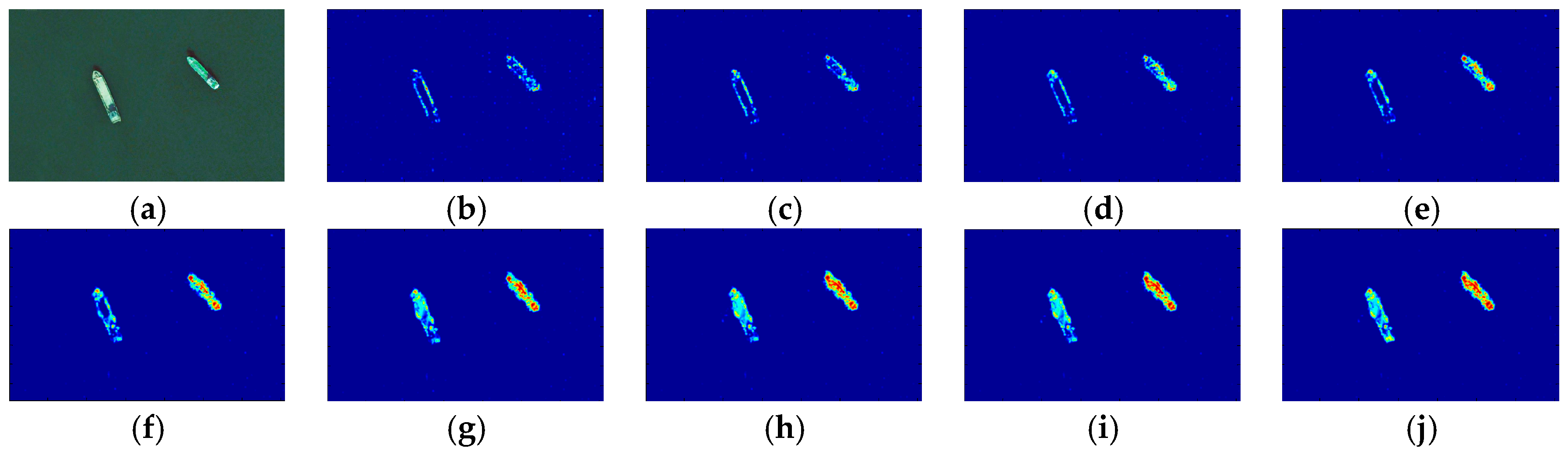
Figure 6.
Binary images with different spatial structures, but with the same histogram.
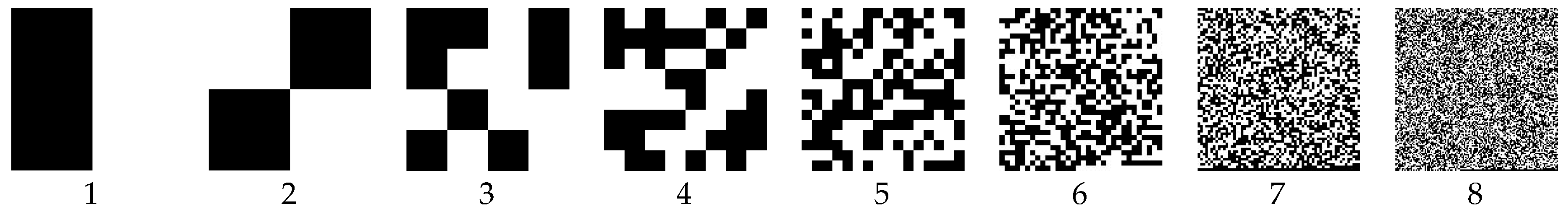
Figure 7.
The entropy values of the eight images using different standard deviations σ.

Figure 8.
The entropy values of the chips.

Figure 9.
Some confusing chips. (a) very few target pixels in the chips, or the edges are covered with clouds; (b) the edges are covered with islands and coasts; and (c) the non-ship targets are inside the chips.
Figure 9.
Some confusing chips. (a) very few target pixels in the chips, or the edges are covered with clouds; (b) the edges are covered with islands and coasts; and (c) the non-ship targets are inside the chips.
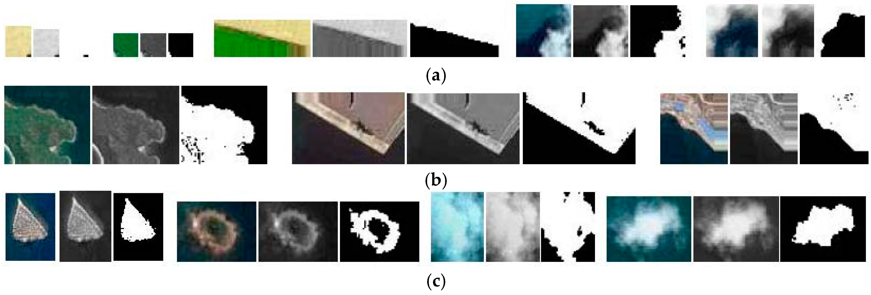
Figure 10.
The illustration for the ten judgment conditions.
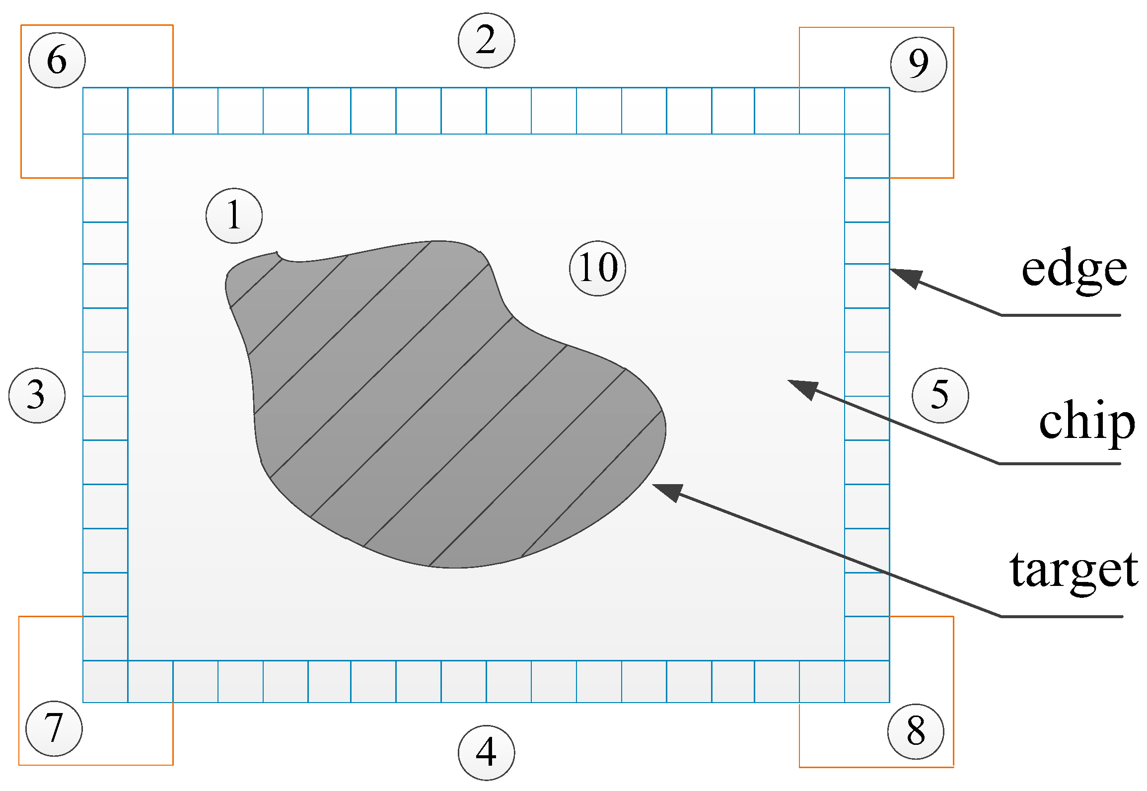
Figure 11.
Visual comparison of the saliency maps: (a) input image; (b) WGS; (c) ITTI; (d) AIM; (e) GBVS; (f) CA; (g) LC; (h) MSSS; (i) SDSP; (j) RARE; (k) SR; and (l) Nevrez.
Figure 11.
Visual comparison of the saliency maps: (a) input image; (b) WGS; (c) ITTI; (d) AIM; (e) GBVS; (f) CA; (g) LC; (h) MSSS; (i) SDSP; (j) RARE; (k) SR; and (l) Nevrez.
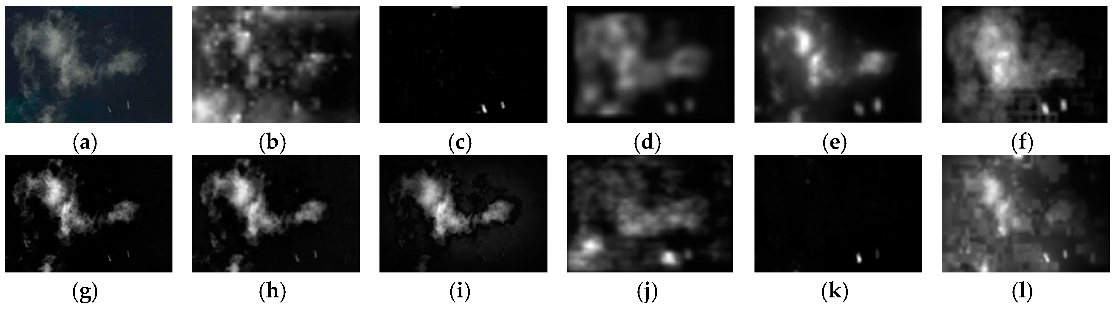

Figure 12.
Visual comparison of the saliency maps: (a) input image; (b) WGS; (c) ITTI; (d) AIM; (e) GBVS; (f) CA; (g) LC; (h) MSSS; (i) SDSP; (j) RARE; (k) SR; and (l) Nevrez.
Figure 12.
Visual comparison of the saliency maps: (a) input image; (b) WGS; (c) ITTI; (d) AIM; (e) GBVS; (f) CA; (g) LC; (h) MSSS; (i) SDSP; (j) RARE; (k) SR; and (l) Nevrez.
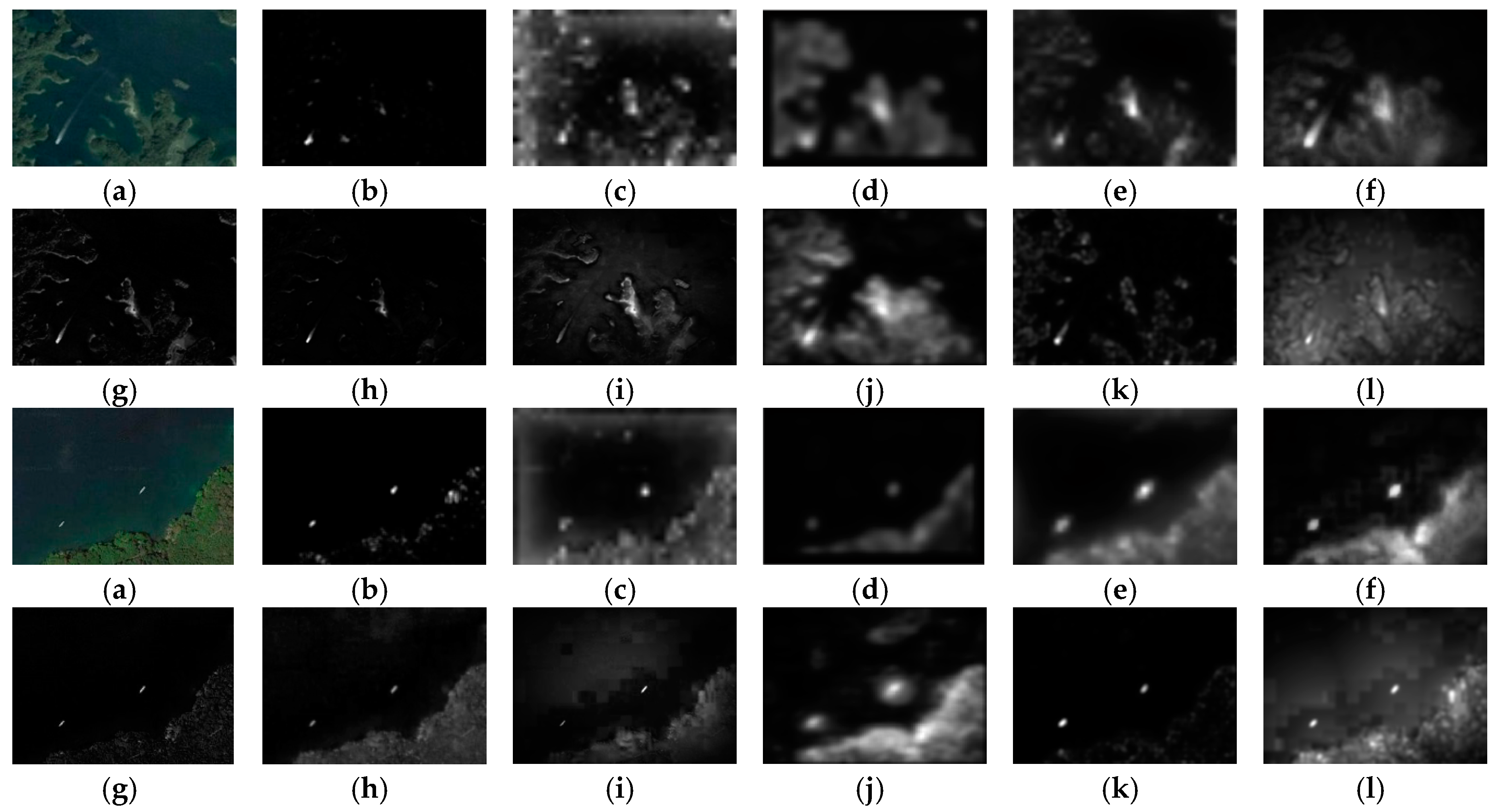
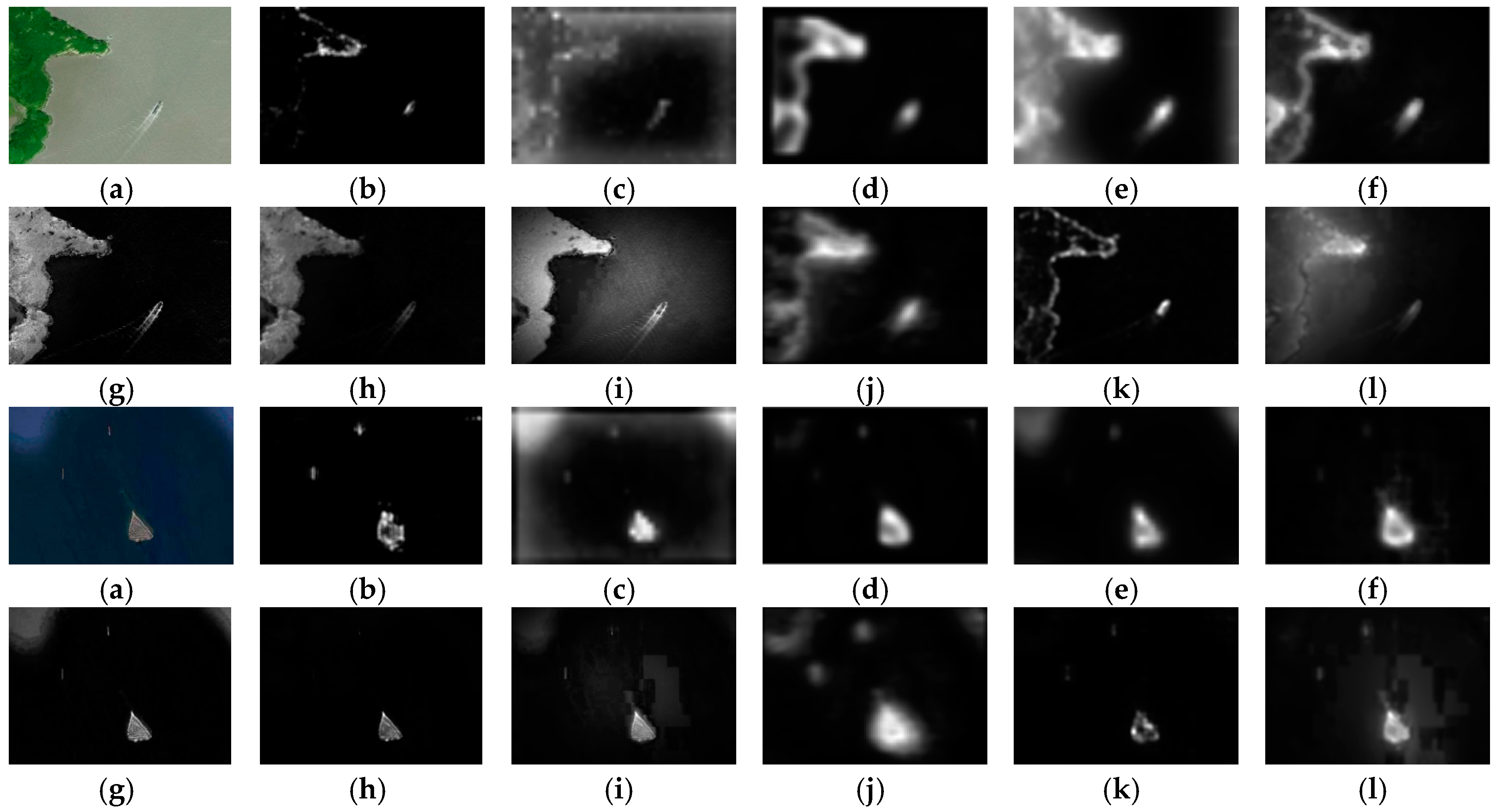
Figure 13.
Some input images and the corresponding ground-truth maps: (a) input images; and (b) ground-truth maps.
Figure 13.
Some input images and the corresponding ground-truth maps: (a) input images; and (b) ground-truth maps.
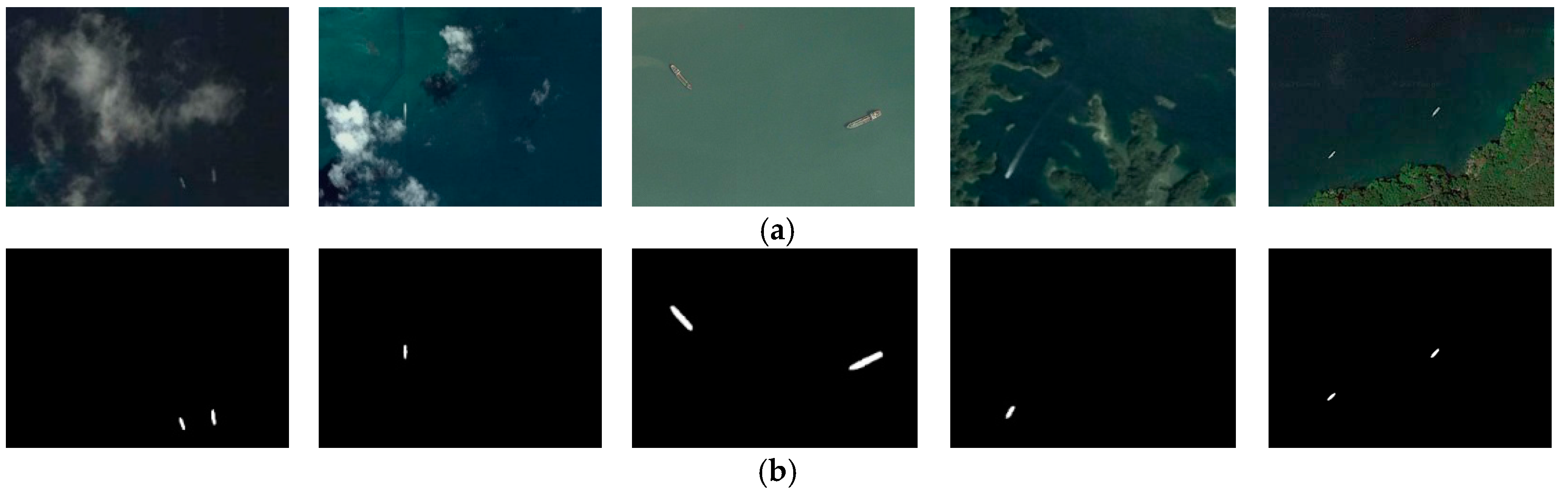
Figure 14.
The ROC curves and the AUC values of different saliency models:(a) ROC curves; and (b) AUC.
Figure 14.
The ROC curves and the AUC values of different saliency models:(a) ROC curves; and (b) AUC.
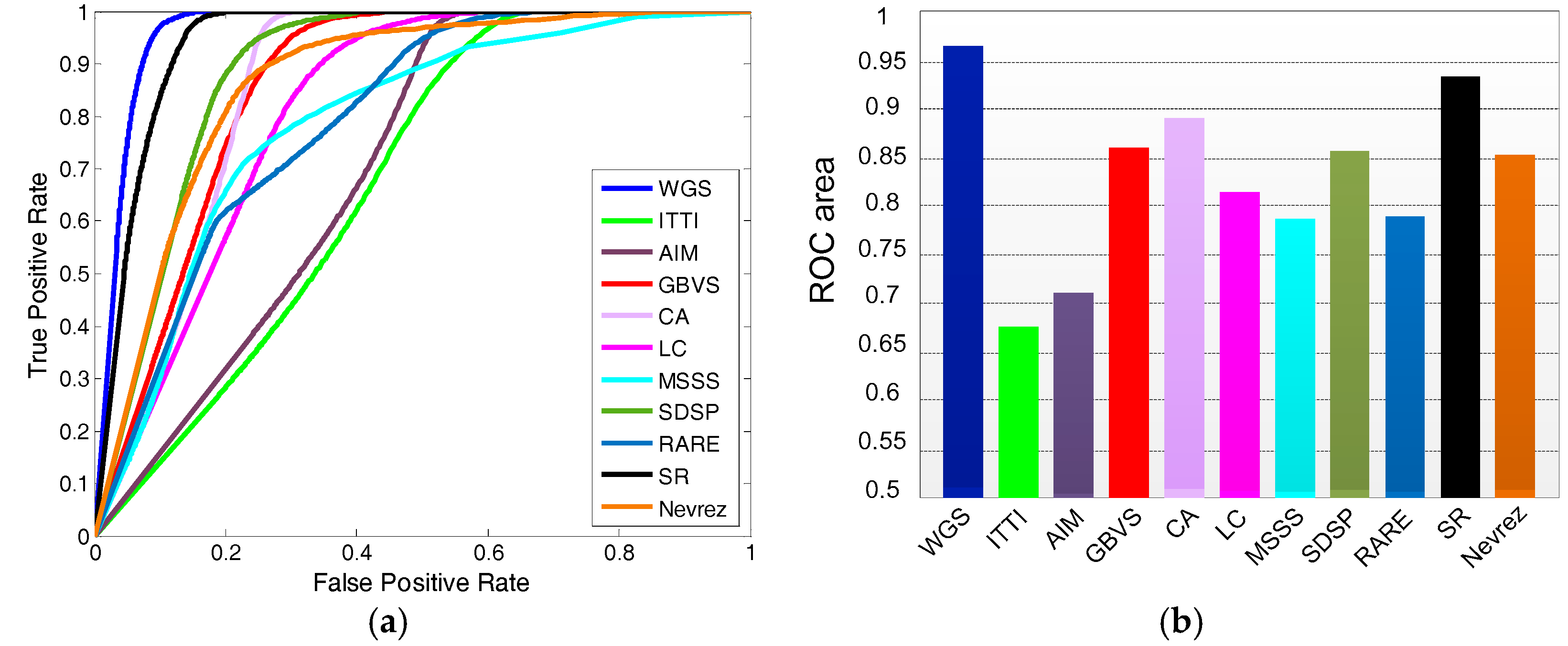
Figure 15.
The detection results for multi-size images. (a) Input image; (b) 300 × 210; (c) 406 × 283; (d) 505 × 354; and (e) 612 × 428.
Figure 15.
The detection results for multi-size images. (a) Input image; (b) 300 × 210; (c) 406 × 283; (d) 505 × 354; and (e) 612 × 428.

Figure 16.
The final detection results after the multi-level discrimination.

Table 1.
Comparisons of the computational time.
| Model | WGS | ITTI | AIM | GBVS | CA | LC | MSSS | SDSP | RARE | SR | Nevrez |
|---|---|---|---|---|---|---|---|---|---|---|---|
| Time (s) | 2.033 | 0.688 | 11.779 | 7.010 | 32.337 | 0.011 | 0.696 | 0.102 | 0.887 | 0.090 | 2.784 |
| Code | M | M | M | M | M | M | M | M | M | M | M |
Table 2.
Effectiveness of the main stages in the proposed method.
| Stage | Nt | Ntt | Nfa | Cr (%) | Far (%) | Mr (%) |
|---|---|---|---|---|---|---|
| WGS | 557 | 540 | 401 | 96.948 | 42.614 | 3.052 |
| SCD | 557 | 535 | 322 | 96.050 | 37.573 | 3.950 |
| IED | 557 | 509 | 69 | 91.382 | 11.938 | 8.618 |
| PDD | 557 | 509 | 31 | 91.382 | 5.741 | 8.618 |
Table 3.
Time cost of main stages in the discrimination (seconds).
| Size | SCD | IED | PDD |
|---|---|---|---|
| 17 × 18 | 9.332 × 10⁻⁷ | 1.9 × 10⁻³ | 2.58 × 10⁻⁴ |
| 51 × 30 | 1.554 × 10⁻⁶ | 3.1 × 10⁻³ | 3.42 × 10⁻⁴ |
| 64 × 64 | 1.867 × 10⁻⁶ | 3.7 × 10⁻³ | 3.93 × 10⁻⁴ |
© 2017 by the authors. Licensee MDPI, Basel, Switzerland. This article is an open access article distributed under the terms and conditions of the Creative Commons Attribution (CC BY) license (http://creativecommons.org/licenses/by/4.0/).
Share and Cite
MDPI and ACS Style
Xu, F.; Liu, J.; Dong, C.; Wang, X. Ship Detection in Optical Remote Sensing Images Based on Wavelet Transform and Multi-Level False Alarm Identification. Remote Sens. 2017, 9, 985. https://doi.org/10.3390/rs9100985
AMA Style
Xu F, Liu J, Dong C, Wang X. Ship Detection in Optical Remote Sensing Images Based on Wavelet Transform and Multi-Level False Alarm Identification. Remote Sensing. 2017; 9(10):985. https://doi.org/10.3390/rs9100985
Chicago/Turabian StyleXu, Fang, Jinghong Liu, Chao Dong, and Xuan Wang. 2017. "Ship Detection in Optical Remote Sensing Images Based on Wavelet Transform and Multi-Level False Alarm Identification" Remote Sensing 9, no. 10: 985. https://doi.org/10.3390/rs9100985
Note that from the first issue of 2016, this journal uses article numbers instead of page numbers. See further details here.