Mapping and Attributing Normalized Difference Vegetation Index Trends for Nepal


1
Department of Civil Engineering and NOAA-CREST, City College of New York, New York, NY 10031, USA
2
The Graduate Center, City University of New York, New York, NY 10016, USA
3
Department of Biology, Queens College, City University of New York, Queens, NY 11367, USA
*
Author to whom correspondence should be addressed.
Remote Sens. 2017, 9(10), 986; https://doi.org/10.3390/rs9100986
Submission received: 8 September 2017
/
Revised: 8 September 2017
/
Accepted: 21 September 2017
/
Published: 23 September 2017
(This article belongs to the Section Remote Sensing in Agriculture and Vegetation)
Abstract
:Global change affects vegetation cover and processes through multiple pathways. Long time series of surface land surface properties derived from satellite remote sensing give unique abilities to observe these changes, particularly in areas with complex topography and limited research infrastructure. Here, we focus on Nepal, a biodiversity hotspot where vegetation productivity is limited by moisture availability (dominated by a summer monsoon) at lower elevations and by temperature at high elevations. We analyze the normalized difference vegetation index (NDVI) from 1981 to 2015 semimonthly, at an 8 km spatial resolution. We use a random forest (RF) of regression trees to generate a statistical model of the NDVI as a function of elevation, land use, CO level, temperature, and precipitation. We find that the NDVI increased over the studied period, particularly at low and middle elevations and during the fall (post-monsoon). We infer from the fitted RF model that the NDVI linear trend is primarily due to CO level (or another environmental parameter that is changing quasi-linearly), and not primarily due to temperature or precipitation trends. On the other hand, interannual fluctuation in the NDVI is more correlated with temperature and precipitation. The RF accurately fits the available data and shows promise for estimating trends and testing hypotheses about their causes.
1. Introduction
Vegetation is being impacted globally by widespread stressors and changes, including land conversion to human uses, climate change leading to heat and moisture stress, CO fertilization, nitrogen deposition, and the spread of pests and invasive species. While methods such as in situ inventories, atmospheric trace-gas measurement, and numerical modeling can provide valuable insights into quantifying and attributing impacts [1,2,3,4,5], remote sensing of the land surface offers a unique avenue for observing changes in vegetation cover over large areas and timespans of days to decades. The normalized difference vegetation index (NDVI), based on the relative surface reflectance in red and near-infrared wavelengths, is well correlated with cover of healthy vegetation [6], and regional and global products based on different satellite sensors are available [7,8]. The NDVI is negatively affected by drought in warm regions [9,10,11] but has increased in response to warming in many temperate and Arctic areas, which has resulted in longer growing seasons there [12,13,14]. For East and Central Asia, the NDVI was found to have increased from approximately 1982 to 1996 as a result of longer growing seasons, and it then decreased from 1997 to 2006 as a result of worsening aridity [15,16]. Urbanization, irrigation and fertilization can also change the NDVI [17,18]. Because the trends in most places are small in magnitude, remote sensing data needs to be carefully processed to remove artifacts due to, for example, degradation of the satellite sensors over the course of a mission [19].
Here, we study trends in the vegetation cover in Nepal (located at 26°N–31°N, 80°E–89°E) a least developed country for which the majority of the population is engaged in agriculture and that is highly vulnerable to climate change. Nepal is a biodiversity hotspot, as a result, in part, of the wide topographic and climatic range found over relatively short distances, ranging from the Indo-Gangetic Plain in the south to the Himalayan peaks and the Tibetan Plateau to the north [20]. Several studies of NDVI trends in the broader region have previously been conducted. A generally increasing trend in the spring NDVI over the Hindu Kush–Himalayan region was found between 1982 and 2006 in [21]. The NDVI seasonality was analyzed in [22] between 1982 and 2006 for the Himalayan region, including Nepal, and it was found that the start date of the growing season trended earlier, while the end date did not change. Cluster analysis was conducted in [23] to identify patterns in the mean and maximum warm-season NDVI between 2001 and 2016; mostly increasing trends (greening) were found, and decreasing trends (browning) were most common between 4 and 5 km elevation. Similarly, a study of NDVI trends in Yarlung Zangbo Grand Canyon Nature Reserve, Tibet between 1999 and 2013 [24] found that greening was concentrated at the lower elevations, below 3 km. Delayed green-up in alpine grasslands of the western Tibetan Plateau may be due to declines in spring precipitation [25,26].
Limited research has been carried out on NDVI trends specifically in Nepal. Forest types in the Manaslu Conservation Area were mapped and NDVI trends and correlations with temperature and precipitation from a nearby meteorological station were computed for 2000–2008 in [27]. A significant increasing trend in the warm-season NDVI over the Koshi River Basin for 1982–2006 was found in [28], although with a decline between 1994 and 2000.
This research, therefore, has two main objectives. First, we describe trends in the NDVI in Nepal by elevation and season on the basis of a long-term remote sensing data product. Second, we attempt to attribute trends and interannual variability to changes in the climate, land use, and CO concentration.
2. Methods
2.1. Data
2.1.1. NDVI
NDVI data was obtained from the NDVI3g.v1 time series, an update of the earlier NDVI3g.v0 [29], which provides NDVI values twice a month on a 1/12 degree (approximately 8 km) grid from July 1981 to December 2015. This dataset is derived from measurements by over a dozen advanced very high resolution radiometers (AVHRRs) that orbited on different satellites for parts of this time period. It has been extensively processed to correct for artifacts resulting from causes such as instrument and orbit drift and volcanic eruptions, so as to be suitable for analysis of climate change. The formula for the NDVI is (NIR − RED)/(NIR + RED), where NIR refers to reflectance in the AVHRR near-infrared band (channel 2; 0.725–1.10 m) and RED, to reflectance in the AVHRR red band (channel 1; 0.58–0.68 m) [30]. Missing or suspect data in NDVI3g.v1 was flagged and filled in either by spline interpolation or from an average of other years.
Despite quality control steps used to derive this product, we found occasional NDVI values that were quite different from those at adjacent time periods, and which were therefore likely to be due to satellite instrument or viewing condition artifacts [31]. We therefore smoothed the NDVI3g.v1 series by subtracting the median seasonal cycle, applying a three-point median filter, and adding the seasonal cycle back.
2.1.2. Elevation
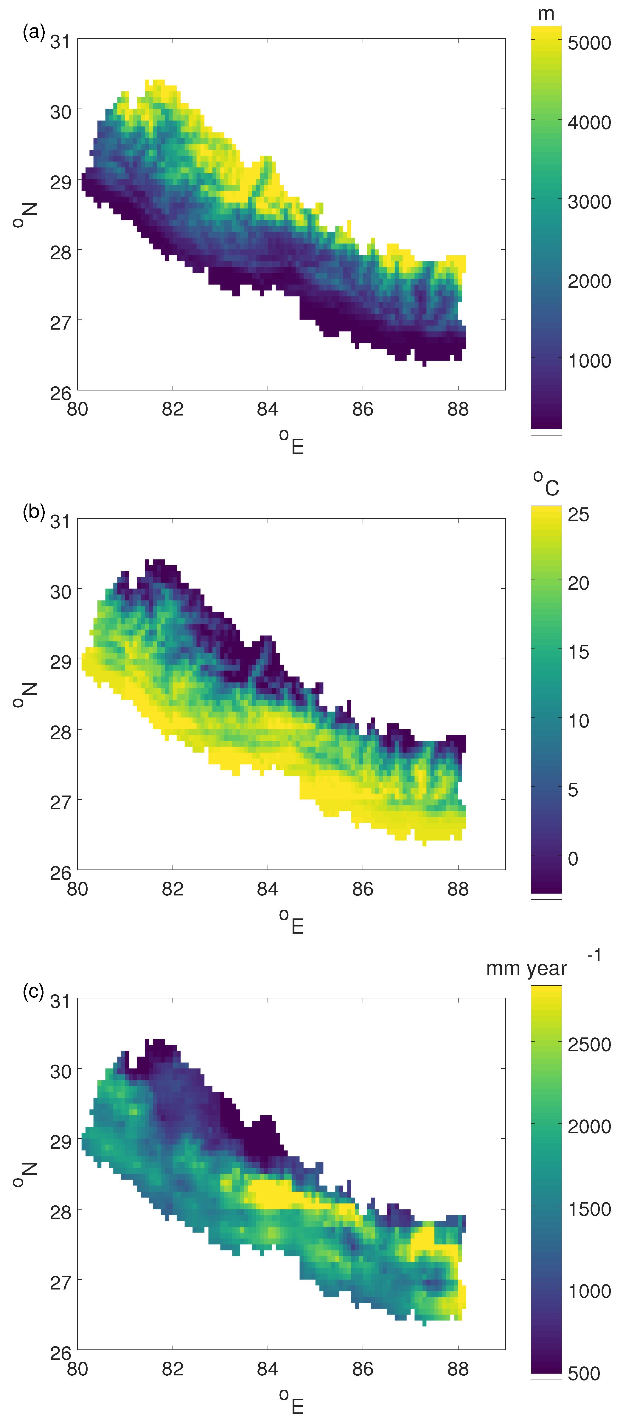
Elevation was obtained at 3 arcsecond (approximately 80 m) resolution from the United States Geological Survey (USGS) and World Wildlife Foundation (WWF) hydrological data and maps based on the Shuttle Elevation Derivatives at multiple Scales (HydroSHEDS) project. HydroSHEDS is derived from spaceborne radar images with extensive quality control and corrections of artifacts [32]. We computed the average and standard deviation of the elevation over each 1/12° grid cell in Nepal as possible predictors of the NDVI. The mean pixel elevations ranged from 60 to over 6000 m (Figure 1a), with an average of 2078 m.
2.1.3. Climate
The monthly mean temperature and precipitation were obtained on a 1° grid. The precipitation was from the Global Precipitation Climatology Center (GPCC) combined Full Version 7 and Monitoring Version 4 product, which is based on quality-controlled data from thousands of stations globally (including data contributed by Nepal through the World Meteorological Organization) that is interpolated to fill in gaps in coverage [33,34,35]. The temperature was from the Berkeley Earth (BEST) dataset, which uses several times the number of station records compared to other gridded temperature datasets. Station records undergo automated quality control and are weighted using geostatistics methods to produce spatial fields [36].
The 1° resolution of these available products does not fully resolve the topography-driven climate variability in Nepal. We mitigated this shortcoming, to some extent, by applying downscaling adjustments. We downscaled the temperature data within each 1° cell to 1/12° by applying a lapse rate of 6 K/km as an additive adjustment. This lapse rate was approximately that inferred from the temperature difference between adjacent BEST pixels, which was found to be approximately the same for all seasons. We downscaled the precipitation data within each 1° cell to 1/12° by applying a multiplicative conversion factor based on the higher-resolution gridded APHRODITE product, available for 1951–2007 in a public version at 0.25° resolution and, courtesy of the Nepal Department of Hydrology and Meteorology, at the original 0.05° interpolation resolution [37]. These adjustment factors were the same for each month, so that time trends were not affected and the 1° mean values from BEST and GPCC were preserved.
The mean temperature and precipitation obtained, along with the mean elevation, for each 1/12° NDVI pixel are shown in Figure 1.
2.1.4. Land Cover
Land cover classifications for 1990, 2000, and 2010 were obtained from the International Centre for Integrated Mountain Development (ICIMOD) [38]. These were generated using public domain Landsat Thematic Mapper 30 m images and an object-based classification algorithm, and they were validated and refined using aerial photographs and field observations. The land cover classes were forest, shrub, grass, agricultural, barren, lake, river, snow/glacier, and urban. We computed the percentage in each cover category for each 1/12° pixel and year. Land cover was imputed by pixel and year via linear interpolation between the three available years. Before 1990 and after 2010, we assumed the land cover to have remained constant at the earliest/latest available value.
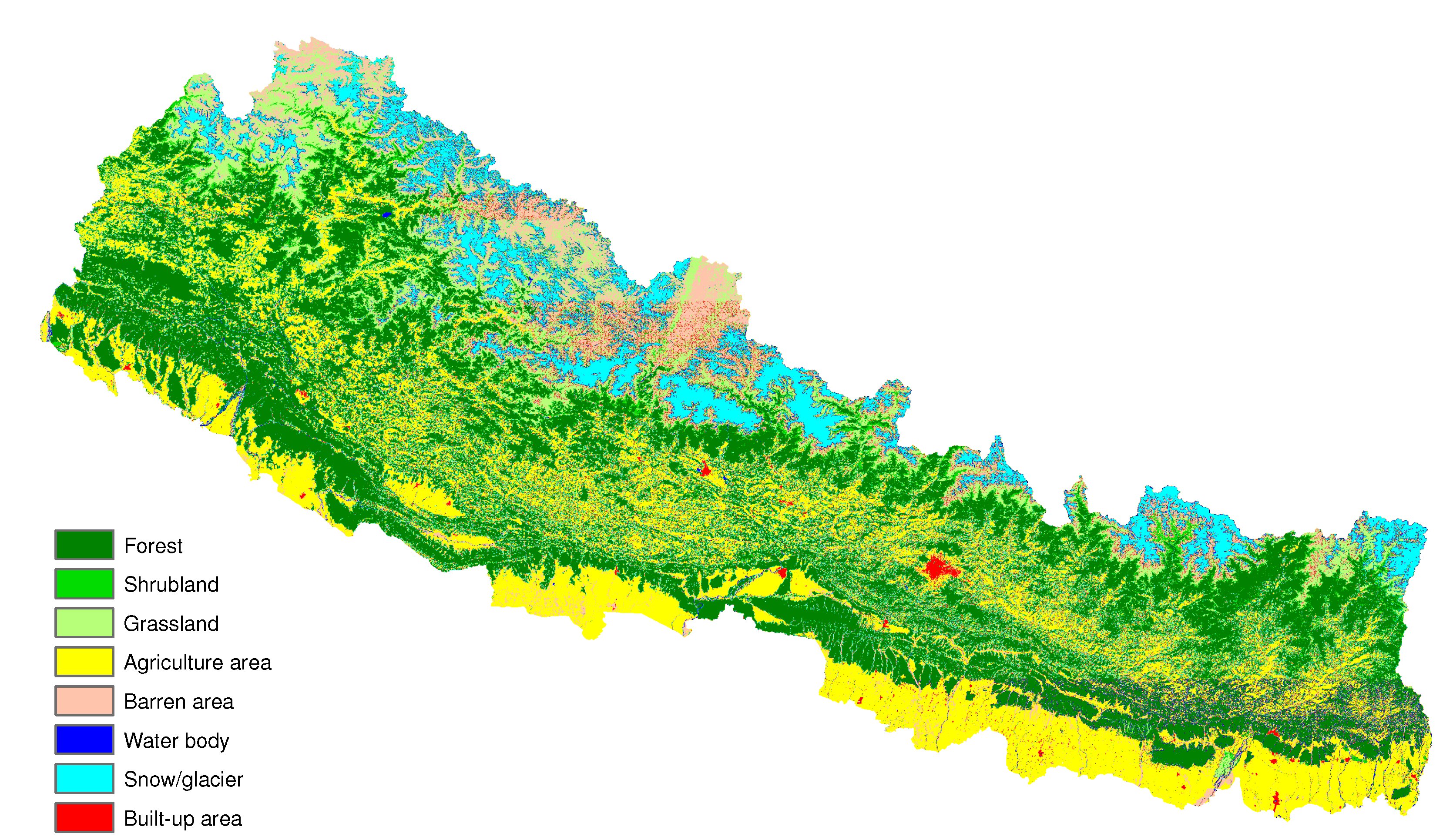
The obtained land cover classification showed that forest (at almost half the area) and agriculture (at about a quarter) were the dominant categories (Table 1). Agriculture dominated in the lowest elevations in the south, while forest dominated in the middle elevations, and grassland, snow and glaciers were found at high elevations in the north (Figure 2). Forest cover decreased by several percentage points between 1990 and 2000, while agricultural and barren areas increased, before stabilizing between 2000 and 2010 (Table 1).
2.1.5. CO Concentration
Yearly carbon dioxide dry air mixing ratios from Mauna Loa, Hawai’i (at 20° North, close to Nepal’s latitude) were obtained from the United States Government Earth System Research Laboratory, Global Monitoring Division. These were transformed to logarithms and can represent the impact of increasing local carbon dioxide levels on the plant gas exchange and carbon fixation. This time series is also highly correlated to the summed anthropogenic greenhouse gas forcing [39], the global warming trend [40], and other monotonic trends over recent decades, such as that of global population [41,42].
2.2. Regression Model
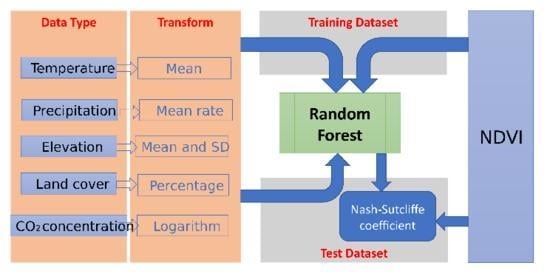
We expect the relationship of the NDVI with such variables as temperature, precipitation and elevation to be nonlinear. There also may well be interactions between potential explanatory variables, for example, the effect of precipitation increase could vary depending on elevation and season. A random forest (RF) of regression trees [43] is a method of empirically constructing a predictive model that is well suited for handling such complexity. As such, RFs have been used in many environmental mapping applications, including for wetland cover from radar imagery [44], water table dynamics and depth to groundwater [45,46], and ecosystem light-use efficiency [47]. Here, the training data were half of the available 1,429,443 NDVI values from Nepal (1955 pixels for 828 time periods, excluding 12% interpolated data). The half the available data not used to train the model (test data) provided a test of its ability to capture the NDVI patterns consistently found by remote sensing. The RF model run included 100 regression trees, and other parameter settings were kept at default values from the R randomForest package [48].
The predictors in the RF model fell into the following categories: (1) Interannually constant seasonal and geographic factors: month of year, pixel longitude, pixel latitude, pixel mean elevation, and pixel standard deviation of elevation. (2) Mean temperature (°C) for 0–0.5, 0.5–1.5, 1.5–3, 3–6, 6–12, 12–24, and 24–48 months prior to the end of each semimonthly period. (3) Precipitation rate (mm/month) over the same periods as for temperature. (4) Land cover: percentage of pixels in each of eight land cover categories. (5) Logarithm of atmospheric CO concentration. The total number of predictors in the model was therefore
We then used the fitted model to predict the NDVI trends if only one factor (temperature, precipitation, land use, or CO) changes with time, while the others are held at average values for the period (in the case of temperature and precipitation, seasonally specific averages). To the extent that these factors have different time histories so that their effects on the NDVI can be separated by the RF model, this would allow us to estimate how much of the NDVI trends and interannual variability over Nepal could be attributed to each factor.
2.3. Analysis
For each grid cell and (semimonthly) time of year, we computed the NDVI trend as the slope obtained from linear regression, using only non-interpolated values. The trends were similarly computed for the RF-predicted NDVI. The Nash–Sutcliffe coefficient [49] (NSC), applied to different transformations of the data, is used to quantify how well the RF models fit test data based on either the full set of forcings or sets that include only one time-changing factor. is based directly on the observed and modeled NDVI values (using only the test data), and is based on the same NDVI values, but after subtracting the linear trend (calculated using both training and test data) for each pixel and time of year, which also removes the mean spatial and seasonal NDVI patterns from consideration. is based on the linear trends, and measures how well the RF model is able to capture the observed trend across space and season.
Figure 3 shows graphically the overall workflow followed, including the relationship between data processing and RF modeling.
As one way of visualizing the results, we computed the time series of the mean NDVI over Nepal by averaging across the pixels at each (bi-monthly) time step, using either the filled-in NDVI or the RF predictions. The mean seasonal cycle was subtracted to obtain a deseasonalized time series for computing trends and detrended variability. We also computed the mean NDVI values and trends by season and elevation, using a smoothing spline [50] to estimate the mean elevation dependence.
3. Results
The mean NDVI was near zero in the dry, cold, high-elevation north of Nepal, which has little vegetation. It was somewhat lower in the low plains near the Indian border, compared to middle elevations, peaking at about 0.65 over the elevation range of 500–2000 m (Figure 4).
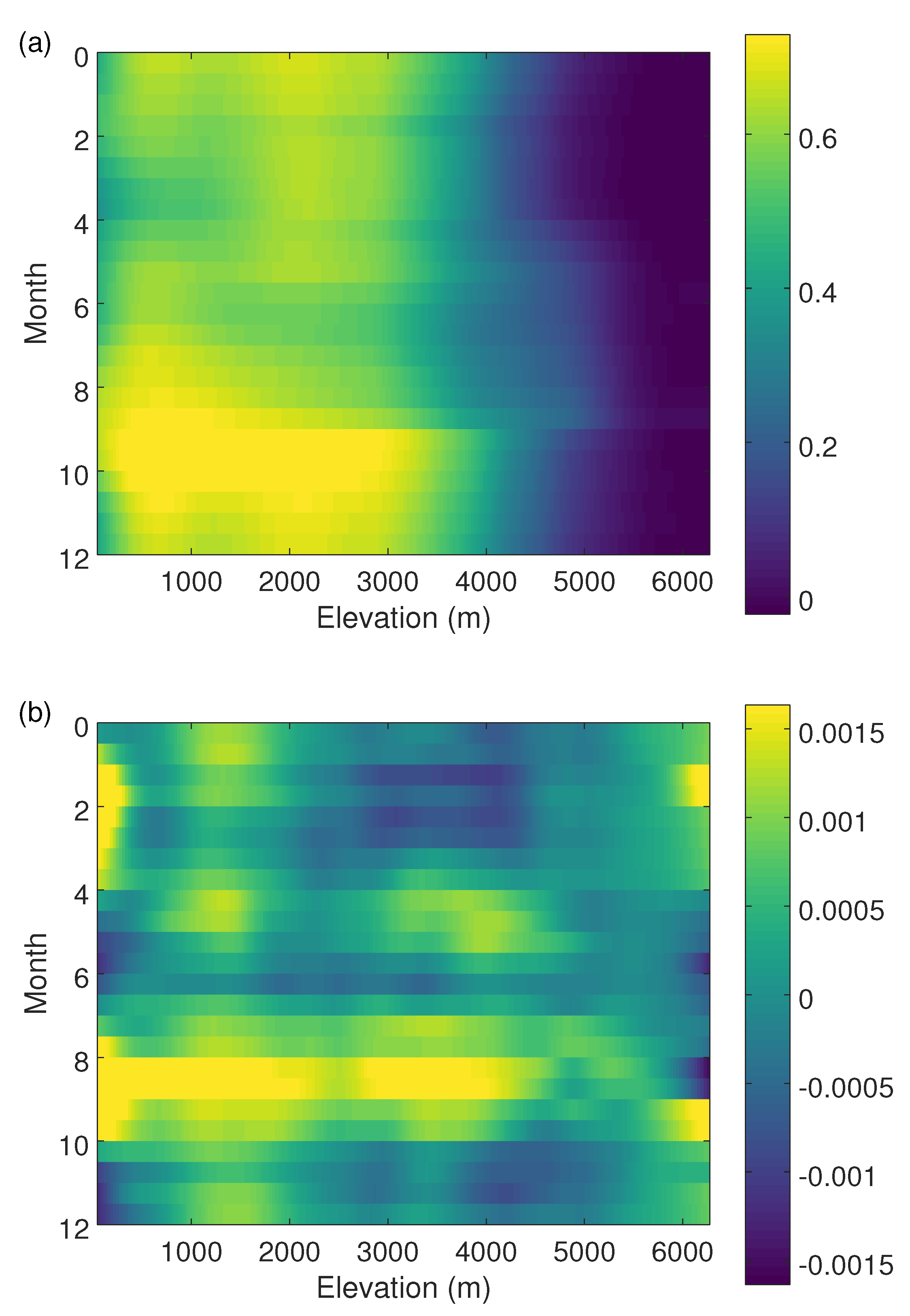
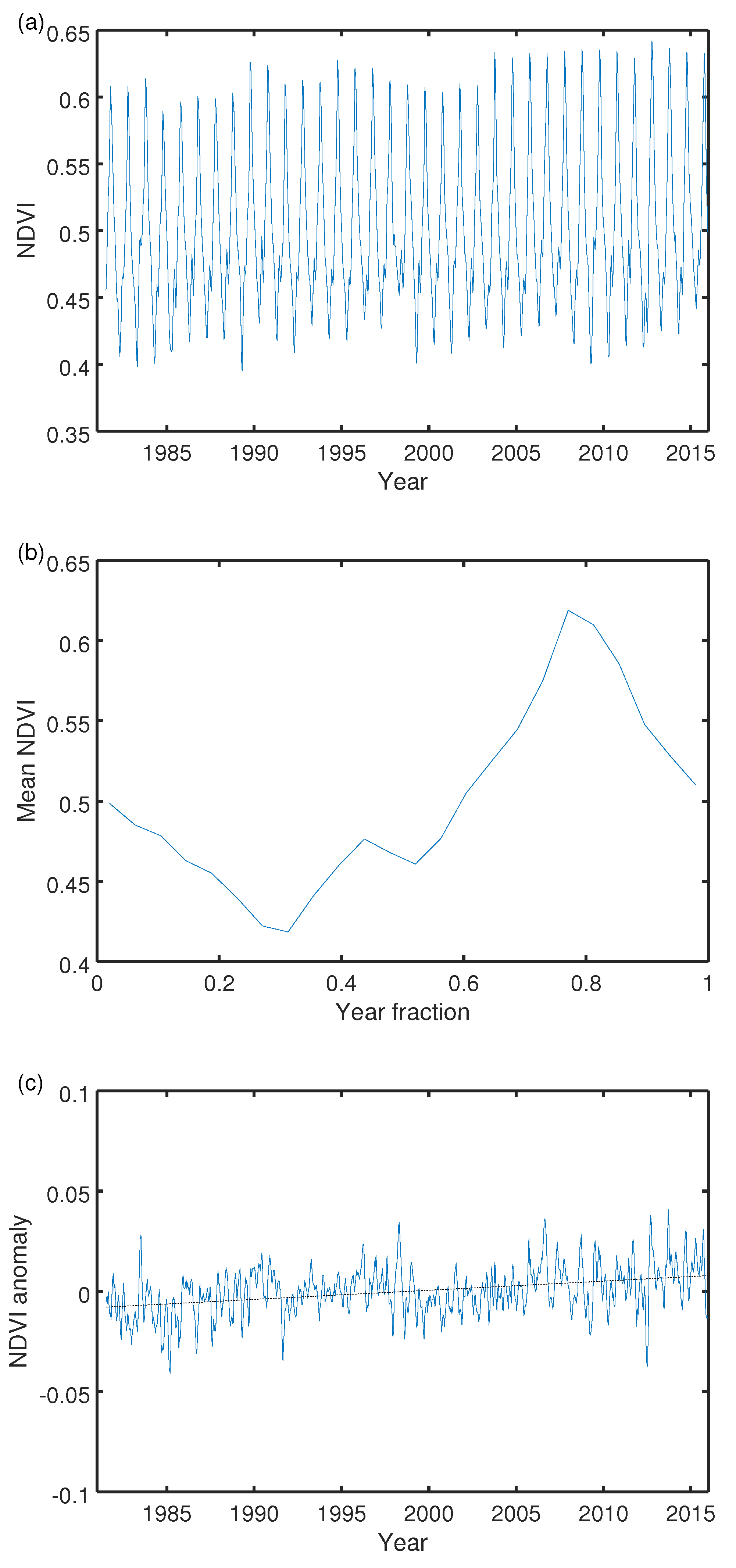
The time series of the mean NDVI is dominated by the seasonal cycle, although interannual variability is also evident (Figure 5). The mean NDVI seasonal cycle nationally and at elevations under ∼4000 m was influenced more by moisture than by temperature, with peak values immediately after the monsoon in early October. The NDVI declined through winter, as water availability decreased, and reached a nadir in late April (Figure 5b; Figure 6a). At higher elevations (4000–5000 m), the peak occurs earlier (late September) and the lowest values are in late February, consistent with a greater role of cold temperature in controlling vegetation cover.
The NDVI overall showed an increasing linear trend, averaging units per year, over the recording period. This trend varied across seasons and elevations, however. It was strongest in late August through October, near the annual peak, and in the lower elevations, below 2000 m (Figure 6b). The NDVI at 4000–5000 m actually showed a slight declining trend.
The RF model was able to represent most of the observed variability in NDVI (Figure 7a), with an value of 0.959 for the test data. However, most of this reflects skill at capturing the mean annual cycle (Figure 7b) and its spatial variation rather than trends and year-to-year variability, so that even with no interannually varying forcings, the value was still 0.941. Out of the single forcings, CO and precipitation contributed most to improving and temperature contributed least (Table 2).
Interannual variability in the NDVI after detrending was less well captured by the RF model (Figure 7c), with a value of 0.288 for the test data. As expected, with no interannually varying forcing, none of this variability was captured. Out of the single forcings, precipitation contributed most to and temperature played a lesser role that was similar in importance to that of the slowly varying CO and land use (Table 2).
The pattern of trends in the NDVI across location and season was better captured by the RF model, with a value of 0.793. With no interannually varying forcing, the trend was uniformly zero, as opposed to the true positive mean value seen, resulting in a slightly negative value. Out of the individual forcings, CO as well as land cover, which both changed quasi-linearly with time, explained the trends best, and trends in temperature and precipitation showed smaller positive values (Table 2).
Averaged over all of Nepal, the mean NDVI trend from the fitted RF model was per year, just 5% less than the calculated from the observation dataset. (Including all pixels and months, also those missing from the observations, increases the mean trend calculated from the fitted RF model slightly to per year.) This mean trend is indicated as being due essentially to a rising CO level, which by itself raises the NDVI by per year. Land cover had a net negative influence on the NDVI trend, while precipitation and temperature trends had small positive influences (Table 2).
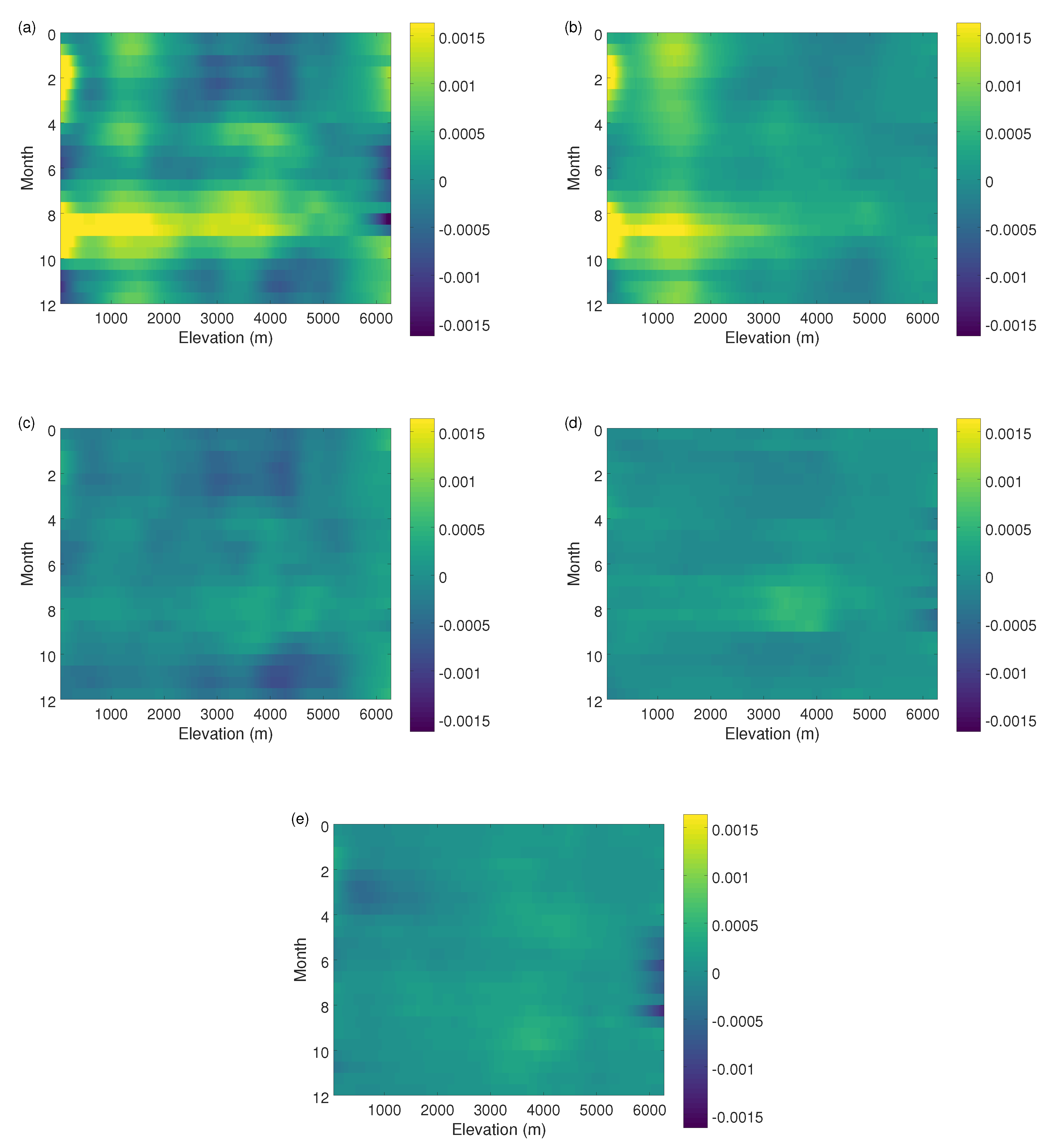
Figure 8 shows the modeled NDVI trend by season and elevation, which can be compared with the observation-based trend in Figure 6b. CO change is the dominant factor for most of the affected seasons and elevations. Land-use change seems to have had the largest impacts, which varied by season, above 2000 m. Precipitation trends impacted the NDVI primarily during the monsoon season of summer and early fall. Temperature trends increased the NDVI in the spring and fall at around 3000–4500 m.
4. Discussion
We found an overall increasing trend in the NDVI for Nepal over 1981–2015. The RF analysis suggests that this trend is not primarily due to changes in climate (temperature and precipitation), but correlates best with an increasing atmospheric CO level, although precipitation and temperature are more important for explaining the interannual NDVI variability. Similarly, ecosystem models suggest that most of the observed increase in the seasonal amplitude of atmospheric CO indicative of increasing plant growth in the Northern Hemisphere over recent decades, is due to CO fertilization, and climate and land-use changes play secondary roles [5]. An increasing trend in global net primary productivity, particularly in tropical forests, has also been identified on the basis of satellite imagery for 1982–1999 and is attributed primarily to CO fertilization [2]. On the other hand, in boreal areas, warming has been a major driver of longer growing seasons and higher productivity [51,52], while in arid and semiarid areas, moisture availability is a primary modulator of vegetation growth [15,53,54,55]. The small positive impact of precipitation on NDVI trends, concentrated during and after the summer monsoon, is consistent with the increasing trend in monsoon precipitation found for recent decades over much of Nepal [56], although dry spells have also increased [57,58].
Land-cover change is inferred to have made a negative contribution to the NDVI trend. This is plausible insofar as the land cover data show a net decrease in the forest area and an increase in the agricultural area, where forest often has a higher and more constant NDVI than agricultural land [59]. Although the importance of anthropogenic land-cover change as a driver of ecological impacts is widely recognized [60,61,62], studies of global and regional NDVI trends over recent decades have generally concentrated on climate drivers without explicitly accounting for the contribution of land-cover change. A RF model offers one method to distinguish the influence of all these factors, which operate simultaneously around the world.
The work presented here has several significant limitations. The NDVI trends attributed to CO level in the RF model could well also reflect contributions from other factors that have been changing quasi-linearly and whose quantitative evolution was not incorporated in the RF model. These may include, for example, nitrogen fertilization as a result of direct application and deposition, irrigation, change in crops planted, management of grasslands and forests, and changes in cloud and aerosols. For most of these terms, more work is needed to understand how they are changing over different parts of Nepal. Additionally, the quality of some of the inputs used could be improved. Land-cover change could be evaluated from Landsat imagery before 1990 and after 2010. A precipitation product at higher resolution, which could be based on remote sensing calibrated to available weather stations, would better resolve the sharp elevation and orographic gradients within Nepal and thus help to clarify the impact of moisture stress [63,64,65].
5. Conclusions
We found that the NDVI increased over the studied period in Nepal, which is consistent with global trends. The increases were uneven and concentrated at low and middle elevations during the fall (post-monsoon). We inferred from the fitted RF model that the NDVI linear trend was primarily due to CO level (or another environmental parameter that changes quasi-linearly), and not primarily due to temperature or precipitation trends. On the other hand, the interannual fluctuation in the NDVI was correlated more with temperature and particularly with precipitation. The RF accurately fit the available data and shows promise for estimating trends in incompletely sampled spatiotemporal remote sensing data, such as the gridded NDVI, and for testing hypotheses about their causes.
Acknowledgments
The authors gratefully acknowledge support from USAID IPM IL under the project “Participatory biodiversity and climate change assessment for integrated pest management in the Chitwan-Annapurna Landscape, Nepal” and from NOAA under grants NA11SEC4810004 and NA15OAR4310080. All statements made are the views of the authors and are not the opinions of the funders or the U.S. government.
Author Contributions
All authors conceived and designed the data analysis and contributed analysis tools. N.Y.K. performed the data analysis and wrote the paper.
Conflicts of Interest
The authors declare no conflict of interest.
References
- Caspersen, J.P.; Pacala, S.W.; Jenkins, J.C.; Hurtt, G.C.; Moorcroft, P.R.; Birdsey, R.A. Contributions of land-use history to carbon accumulation in U.S. forests. Science 2000, 290, 1148–1151. [Google Scholar] [CrossRef] [PubMed]
- Friend, A.D.; Arneth, A.; Kiang, N.Y.; Lomas, M.; Ogée, J.; Rödenbeck, C.; Running, S.W.; Santaren, J.D.; Sitch, S.; Viovy, N.; et al. FLUXNET and modelling the global carbon cycle. Glob. Chang. Biol. 2007, 13, 610–633. [Google Scholar] [CrossRef]
- Mercado, L.M.; Bellouin, N.; Sitch, S.; Boucher, O.; Huntingford, C.; Wild, M.; Cox, P.M. Impact of changes in diffuse radiation on the global land carbon sink. Nature 2009, 458, 1014–1017. [Google Scholar] [CrossRef] [PubMed] [Green Version]
- McMahon, S.M.; Parker, G.G.; Miller, D.R. Evidence for a recent increase in forest growth. Proc. Natl. Acad. Sci. USA 2010, 107, 3611–3615. [Google Scholar] [CrossRef] [PubMed]
- Zhao, F.; Zeng, N.; Asrar, G.; Friedlingstein, P.; Ito, A.; Jain, A.; Kalnay, E.; Kato, E.; Koven, C.D.; Poulter, B.; et al. Role of CO2, climate and land use in regulating the seasonal amplitude increase of carbon fluxes in terrestrial ecosystems: A multimodel analysis. Biogeosciences 2016, 13, 5121–5137. [Google Scholar] [CrossRef]
- Myneni, R.B.; Hall, F.G.; Sellers, P.J.; Marshak, A.L. The interpretation of spectral vegetation indexes. IEEE Trans. Geosci. Remote Sens. 1995, 33, 481–486. [Google Scholar] [CrossRef]
- Buermann, W.; Wang, Y.; Dong, J.; Zhou, L.; Zeng, X.; Dickinson, R.E.; Potter, C.S.; Myneni, R.B. Analysis of a multiyear global vegetation leaf area index data set. J. Geophys. Res. 2002, 107, 4646. [Google Scholar] [CrossRef]
- Tucker, C.; Pinzon, J.; Brown, M.; Slayback, D.; Pak, E.; Mahoney, R.; Vermote, E.; El Saleous, N. An extended AVHRR 8-km NDVI dataset compatible with MODIS and SPOT vegetation NDVI data. Int. J. Remote Sens. 2005, 26, 4485–4498. [Google Scholar] [CrossRef]
- Narasimha Rao, P.V.; Venkataratnam, L.; Krishna Rao, P.V.; Ramana, K.V.; Singarao, M.N. Relation between root zone soil moisture and normalized difference vegetation index of vegetated fields. Int. J. Remote Sens. 1993, 14, 441–449. [Google Scholar] [CrossRef]
- Zaitchik, B.F.; Evans, J.P.; Geerken, R.A.; Smith, R.B. Climate and vegetation in the Middle East: interannual variability and drought feedbacks. J. Clim. 2007, 20, 3924–3941. [Google Scholar] [CrossRef]
- Schnur, M.T.; Xie, H.; Wang, X. Estimating root zone soil moisture at distant sites using MODIS NDVI and EVI in a semi-arid region of southwestern USA. Ecol. Inform. 2010, 5, 400–409. [Google Scholar] [CrossRef]
- Zhou, L.; Tucker, C.J.; Kaufmann, R.K.; Slayback, D.; Shabanov, N.V.; Myneni, R.B. Variations in northern vegetation activity inferred from satellite data of vegetation index during 1981 to 1999. J. Geophys. Res. 2001, 106, 20069–20084. [Google Scholar] [CrossRef]
- Zhou, L.; Kaufmann, R.K.; Tian, Y.; Myneni, R.B.; Tucker, C.J. Relation between interannual variations in satellite measures of northern forest greenness and climate between 1982 and 1999. J. Geophys. Res. 2003, 108, 4004. [Google Scholar] [CrossRef]
- Churkina, G.; Schimel, D.; Braswell, B.H.; Xiao, X. Spatial analysis of growing season length control over net ecosystem exchange. Glob. Chang. Biol. 2005, 11, 1777–1787. [Google Scholar] [CrossRef]
- Park, H.S.; Sohn, B.J. Recent trends in changes of vegetation over East Asia coupled with temperature and rainfall variations. J. Geophys. Res. 2010, 115, D14101. [Google Scholar] [CrossRef]
- Xu, H.J.; Wang, X.P.; Yang, T.B. Trend shifts in satellite-derived vegetation growth in Central Eurasia, 1982–2013. Sci. Total Environ. 2017, 579, 1658–1674. [Google Scholar] [CrossRef] [PubMed]
- Piao, S.; Fang, J.; Zhou, L.; Guo, Q.; Henderson, M.; Ji, W.; Li, Y.; Tao, S. Interannual variations of monthly and seasonal normalized difference vegetation index (NDVI) in China from 1982 to 1999. J. Geophys. Res. 2003, 108, 4401. [Google Scholar] [CrossRef]
- Milesi, C.; Samanta, A.; Hashimoto, H.; Kumar, K.K.; Ganguly, S.; Thenkabail, P.S.; Srivastava, A.N.; Nemani, R.R.; Myneni, R.B. Decadal variations in NDVI and food production in India. Remote Sens. 2010, 2, 758–776. [Google Scholar] [CrossRef]
- Zhang, Y.; Song, C.; Band, L.E.; Sun, G.; Li, J. Reanalysis of global terrestrial vegetation trends from MODIS products: Browning or greening? Remote Sens. Environ. 2017, 191, 145–155. [Google Scholar] [CrossRef]
- Shrestha, A.B.; Aryal, R. Climate change in Nepal and its impact on Himalayan glaciers. Reg. Environ. Chang. 2011, 11, 65–77. [Google Scholar] [CrossRef]
- Panday, P.K.; Ghimire, B. Time-series analysis of NDVI from AVHRR data over the Hindu Kush–Himalayan region for the period 1982–2006. Int. J. Remote Sens. 2012, 33, 6710–6721. [Google Scholar] [CrossRef]
- Shrestha, U.B.; Gautam, S.; Bawa, K.S. Widespread Climate Change in the Himalayas and Associated Changes in Local Ecosystems. PLOS ONE 2012, 7, 1–10. [Google Scholar] [CrossRef] [PubMed] [Green Version]
- Mishra, N.B.; Mainali, K.P. Greening and browning of the Himalaya: Spatial patterns and the role of climatic change and human drivers. Sci. Total Environ. 2017, 587–588, 326–339. [Google Scholar] [CrossRef] [PubMed]
- Li, H.; Jiang, J.; Chen, B.; Li, Y.; Xu, Y.; Shen, W. Pattern of NDVI-based vegetation greening along an altitudinal gradient in the eastern Himalayas and its response to global warming. Environ. Monit. Assess. 2016, 188, 186. [Google Scholar] [CrossRef] [PubMed]
- Shen, M.; Zhang, G.; Cong, N.; Wang, S.; Kong, W.; Piao, S. Increasing altitudinal gradient of spring vegetation phenology during the last decade on the Qinghai–Tibetan Plateau. Agric. For. Meteorol. 2014, 189–190, 71–80. [Google Scholar] [CrossRef]
- Wang, C.; Guo, H.; Zhang, L.; Liu, S.; Qiu, Y.; Sun, Z. Assessing phenological change and climatic control of alpine grasslands in the Tibetan Plateau with MODIS time series. Int. J. Biometeorol. 2015, 59, 11–23. [Google Scholar] [CrossRef] [PubMed]
- Mainali, J.; All, J.; Jha, P.K.; Bhuju, D.R. Responses of montane forest to climate variability in the central Himalayas of Nepal. Mt. Res. Dev. 2015, 35, 66–77. [Google Scholar] [CrossRef]
- Zhang, Y.; Gao, J.; Liu, L.; Wang, Z.; Ding, M.; Yang, X. NDVI-based vegetation changes and their responses to climate change from 1982 to 2011: A case study in the Koshi River Basin in the middle Himalayas. Glob. Planet. Chang. 2013, 108, 139–148. [Google Scholar] [CrossRef]
- Pinzon, J.E.; Tucker, C.J. A Non-Stationary 1981–2012 AVHRR NDVI3g Time Series. Remote Sens. 2014, 6, 6929–6960. [Google Scholar] [CrossRef]
- Tucker, C.J. Red and photographic infrared linear combinations for monitoring vegetation. Remote Sens. Environ. 1979, 8, 127–150. [Google Scholar] [CrossRef]
- Kogan, F.N. Global drought watch from space. Bull. Am. Meteorol. Soc. 1997, 78, 621–636. [Google Scholar] [CrossRef]
- Lehner, B.; Verdin, K.; Jarvis, A. New global hydrography derived from spaceborne elevation data. Eos Trans. Am. Geophys. Union 2008, 89, 93–94. [Google Scholar] [CrossRef]
- Becker, A.; Finger, P.; Meyer-Christoffer, A.; Rudolf, B.; Schamm, K.; Schneider, U.; Ziese, M. A description of the global land-surface precipitation data products of the Global Precipitation Climatology Centre with sample applications including centennial (trend) analysis from 1901-present. Earth Syst. Sci. Data 2013, 5, 71–99. [Google Scholar] [CrossRef]
- Schneider, U.; Ziese, M.; Meyer-Christoffer, A.; Finger, P.; Rustemeier, E.; Becker, A. The new portfolio of global precipitation data products of the Global Precipitation Climatology Centre suitable to assess and quantify the global water cycle and resources. Proc. Int. Assoc. Hydrol. Sci. 2016, 374, 29–34. [Google Scholar] [CrossRef]
- Schneider, U.; Finger, P.; Meyer-Christoffer, A.; Rustemeier, E.; Ziese, M.; Becker, A. Evaluating the hydrological cycle over land using the newly-corrected precipitation climatology from the Global Precipitation Climatology Centre (GPCC). Atmosphere 2017, 8, 52. [Google Scholar] [CrossRef]
- Rohde, R.; Muller, R.; Jacobsen, R.; Perlmutter, S.; Rosenfeld, A.; Wurtele, J.; Curry, J.; Wickham, C.; Mosher, S. Berkeley Earth temperature averaging process. Geoinform. Geostat. Overv. 2013, 1, 1000103. [Google Scholar] [CrossRef]
- Yatagai, A.; Kamiguchi, K.; Arakawa, O.; Hamada, A.; Yasutomi, N.; Kitoh, A. APHRODITE: Constructing a long-term daily gridded precipitation dataset for Asia based on a dense network of rain gauges. Bull. Am. Meteorol. Soc. 2012, 93, 1401–1415. [Google Scholar] [CrossRef]
- Uddin, K.; Shrestha, H.L.; Murthy, M.; Bajracharya, B.; Shrestha, B.; Gilani, H.; Pradhan, S.; Dangol, B. Development of 2010 national land cover database for the Nepal. J. Environ. Manag. 2015, 148, 82–90. [Google Scholar] [CrossRef] [PubMed]
- Hofmann, D.J.; Butler, J.H.; Dlugokencky, E.J.; Elkins, J.W.; Masarie, K.; Montzka, S.A.; Tans, P. The role of carbon dioxide in climate forcing from 1979 to 2004: Introduction of the Annual Greenhouse Gas Index. Tellus B 2006, 58, 614–619. [Google Scholar] [CrossRef]
- Rohde, R.; Muller, R.A.; Jacobsen, R.; Muller, E.; Perlmutter, S.; Rosenfeld, A.; Wurtele, J.; Groom, D.; Wickham, C. A new estimate of the average Earth surface land temperature spanning 1753 to 2011. Geoinform. Geostat. Overv. 2013, 1, 1000101. [Google Scholar]
- Raupach, M.R.; Marland, G.; Ciais, P.; Le Quere, C.; Canadell, J.G.; Klepper, G.; Field, C.B. Global and regional drivers of accelerating CO2 emissions. Proc. Natl. Acad. Sci. USA 2007, 104, 10288–10293. [Google Scholar] [CrossRef] [PubMed]
- Hofmann, D.J.; Butler, J.H.; Tans, P.P. A new look at atmospheric carbon dioxide. Atmos. Environ. 2009, 43, 2084–2086. [Google Scholar] [CrossRef]
- Breiman, L. Random forests. Mach. Learn. 2001, 45, 5–32. [Google Scholar] [CrossRef]
- Whitcomb, J.; Moghaddam, M.; McDonald, K.; Kellndorfer, J.; Podest, E. Mapping vegetated wetlands of Alaska using L-band radar satellite imagery. Can. J. Remote Sens. 2009, 35, 54–72. [Google Scholar] [CrossRef]
- Bachmair, S.; Weiler, M. Hillslope characteristics as controls of subsurface flow variability. Hydrol. Earth Syst. Sci. 2012, 16, 3699–3715. [Google Scholar] [CrossRef] [Green Version]
- Pérez Hoyos, I.C.; Krakauer, N.Y.; Khanbilvardi, R. Estimating the probability of vegetation to be groundwater dependent based on the evaluation of tree models. Environments 2016, 3, 9. [Google Scholar] [CrossRef]
- Wei, S.; Yi, C.; Fang, W.; Hendrey, G. A global study of GPP focusing on light-use efficiency in a random forest regression model. Ecosphere 2017, 8, e01724. [Google Scholar] [CrossRef]
- Liaw, A.; Wiener, M. Classification and regression by randomForest. R News 2002, 2, 18–22. [Google Scholar]
- Nash, J.; Sutcliffe, J. River flow forecasting through conceptual models part I—A discussion of principles. J. Hydrol. 1970, 10, 282–290. [Google Scholar] [CrossRef]
- Krakauer, N.Y. Estimating climate trends: Application to United States plant hardiness zones. Adv. Meteorol. 2012, 2012, 404876. [Google Scholar] [CrossRef]
- Tucker, C.J.; Slayback, D.A.; Pinzon, J.E.; Los, S.O.; Myneni, R.B.; Taylor, M.G. Higher northern latitude normalized difference vegetation index and growing season trends from 1982 to 1999. Int. J. Biometeorol. 2001, 45, 184–190. [Google Scholar] [CrossRef] [PubMed]
- Bunn, A.G.; Goetz, S.J.; Fiske, G.J. Observed and predicted responses of plant growth to climate across Canada. Geophys. Res. Lett. 2005, 32, L16710. [Google Scholar] [CrossRef]
- Girardin, M.P.; Raulier, F.; Bernier, P.Y.; Tardif, J.C. Response of tree growth to a changing climate in boreal central Canada: A comparison of empirical, process-based, and hybrid modelling approaches. Ecol. Model. 2008, 213, 209–228. [Google Scholar] [CrossRef]
- Yi, C.; Rustic, G.; Xu, X.; Wang, J.; Dookie, A.; Wei, S.; Hendrey, G.; Ricciuto, D.; Meyers, T.; Nagy, Z.; et al. Climate extremes and grassland potential productivity. Environ. Res. Lett. 2012, 7, 035703. [Google Scholar] [CrossRef]
- Allen, C.D.; Breshears, D.D.; McDowell, N.G. On underestimation of global vulnerability to tree mortality and forest die-off from hotter drought in the Anthropocene. Ecosphere 2015, 6, 1–55. [Google Scholar] [CrossRef]
- Panthi, J.; Dahal, P.; Shrestha, M.L.; Aryal, S.; Krakauer, N.Y.; Pradhanang, S.M.; Lakhankar, T.; Jha, A.K.; Sharma, M.; Karki, R. Spatial and temporal variability of rainfall in the Gandaki River Basin of Nepal Himalaya. Climate 2015, 3, 210–226. [Google Scholar] [CrossRef]
- Dahal, P.; Shrestha, N.; Shrestha, M.; Krakauer, N.; Panthi, J.; Pradhanang, S.; Jha, A.; Lakhankar, T. Drought risk assessment in central Nepal: temporal and spatial analysis. Nat. Hazards 2016, 80, 1913–1932. [Google Scholar] [CrossRef]
- Karki, R.; Hasson, S.U.; Schickhoff, U.; Scholten, T.; Böhner, J. Rising precipitation extremes across Nepal. Climate 2017, 5, 4. [Google Scholar] [CrossRef]
- DeFries, R.S.; Field, C.B.; Fung, I.; Collatz, G.J.; Bounoua, L. Combining satellite data and biogeochemical models to estimate global effects of human-induced land cover change on carbon emissions and primary productivity. Glob. Biogeochem. Cycles 1999, 13, 803–815. [Google Scholar] [CrossRef]
- Pettorelli, N.; Vik, J.O.; Mysterud, A.; Gaillard, J.M.; Tucker, C.J.; Stenseth, N.C. Using the satellite-derived NDVI to assess ecological responses to environmental change. Trends Ecol. Evolut. 2005, 20, 503–510. [Google Scholar] [CrossRef] [PubMed]
- Foley, J.A.; DeFries, R.; Asner, G.P.; Barford, C.; Bonan, G.; Carpenter, S.R.; Chapin, F.S.; Coe, M.T.; Daily, G.C.; Gibbs, H.K.; et al. Global Consequences of Land Use. Science 2005, 309, 570–574. [Google Scholar] [CrossRef] [PubMed]
- De Jong, R.; Verbesselt, J.; Schaepman, M.E.; de Bruin, S. Trend changes in global greening and browning: Contribution of short-term trends to longer-term change. Glob. Chang. Biol. 2012, 18, 642–655. [Google Scholar] [CrossRef]
- Krakauer, N.Y.; Pradhanang, S.M.; Lakhankar, T.; Jha, A.K. Evaluating satellite products for precipitation estimation in mountain regions: A case study for Nepal. Remote Sens. 2013, 5, 4107–4123. [Google Scholar] [CrossRef]
- Yatagai, A.; Krishnamurti, T.N.; Kumar, V.; Mishra, A.K.; Simon, A. Use of APHRODITE rain gauge–based precipitation and TRMM 3B43 products for improving Asian monsoon seasonal precipitation forecasts by the superensemble method. J. Clim. 2014, 27, 1062–1069. [Google Scholar] [CrossRef]
- Krakauer, N.Y.; Pradhanang, S.M.; Panthi, J.; Lakhankar, T.; Jha, A.K. Probabilistic precipitation estimation with a satellite product. Climate 2015, 3, 329–348. [Google Scholar] [CrossRef]
Figure 1.
Mean pixel (a) elevation, (b) temperature, and (c) precipitation.

Figure 2.
Land cover map of Nepal in 2010.

Figure 3.
Overall structure of data and analysis workflow.
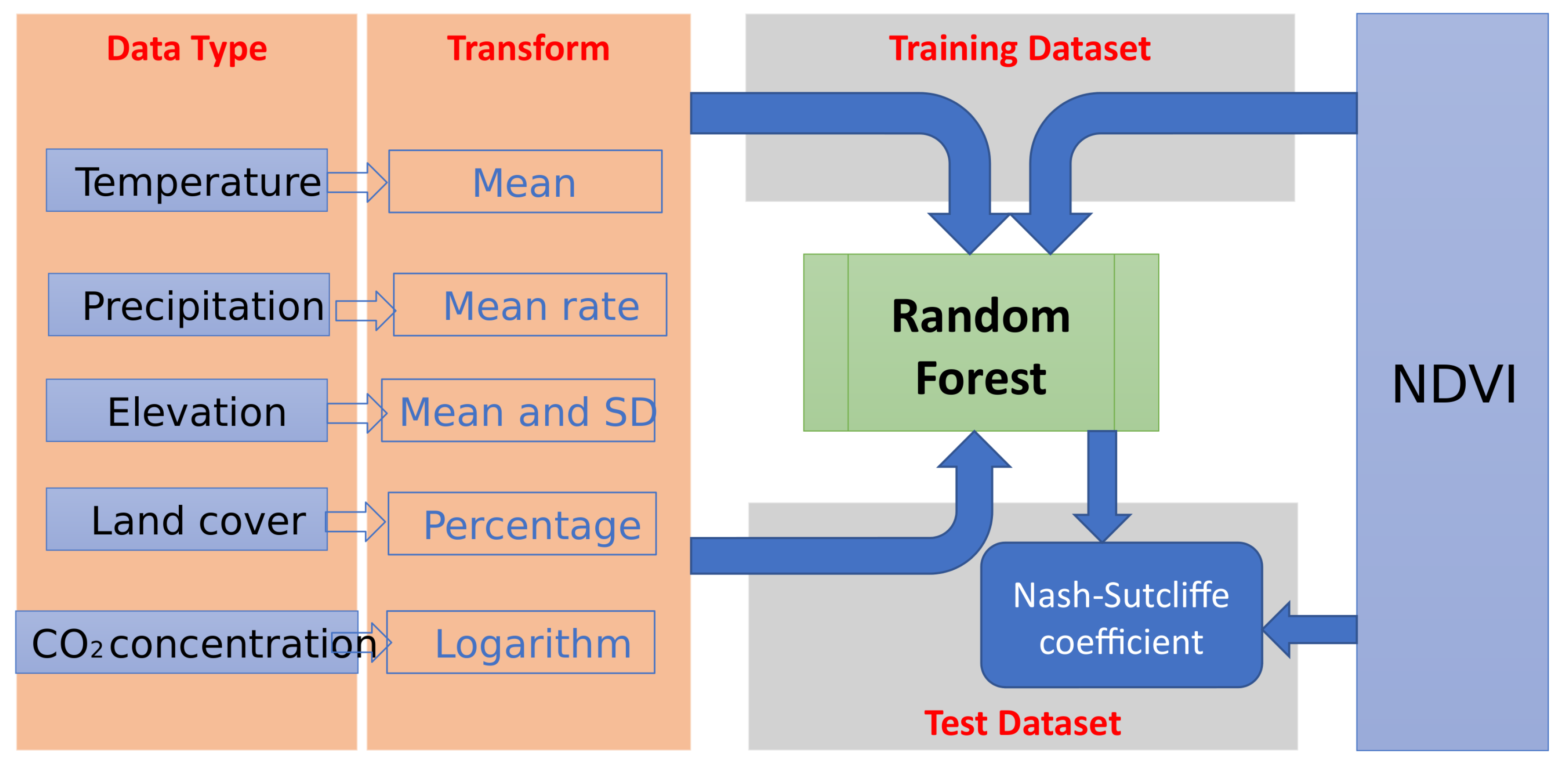
Figure 4.
Mean normalized difference vegetation index (NDVI) by pixel over Nepal.
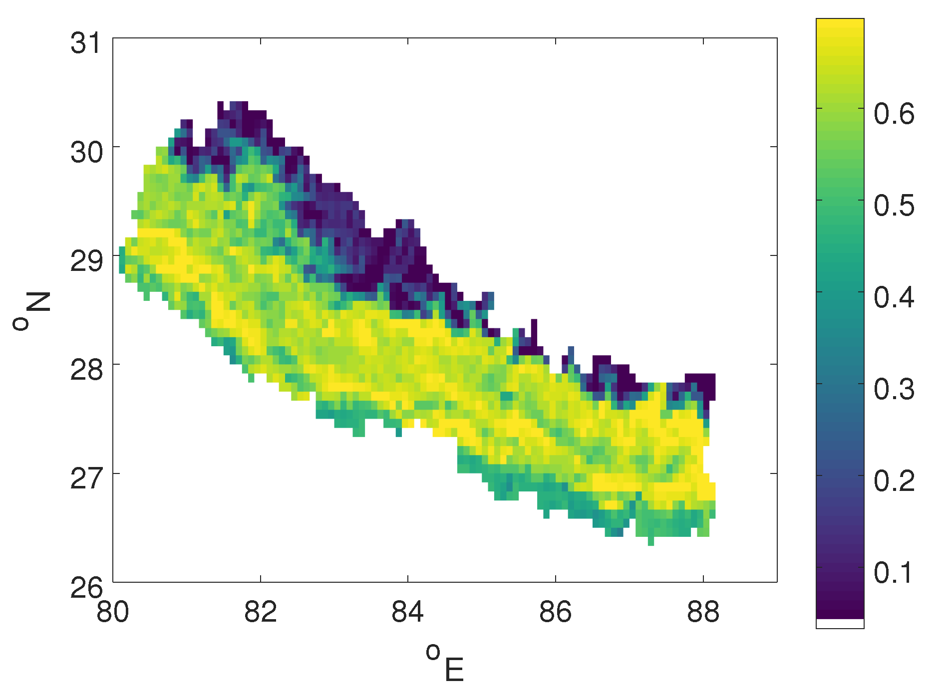
Figure 5.
(a) Time series of mean Nepal normalized difference vegetation index (NDVI). (b) Mean seasonal cycle of NDVI. (c) NDVI anomaly (subtracting the mean seasonal cycle) and its least-squares linear fit.
Figure 5.
(a) Time series of mean Nepal normalized difference vegetation index (NDVI). (b) Mean seasonal cycle of NDVI. (c) NDVI anomaly (subtracting the mean seasonal cycle) and its least-squares linear fit.
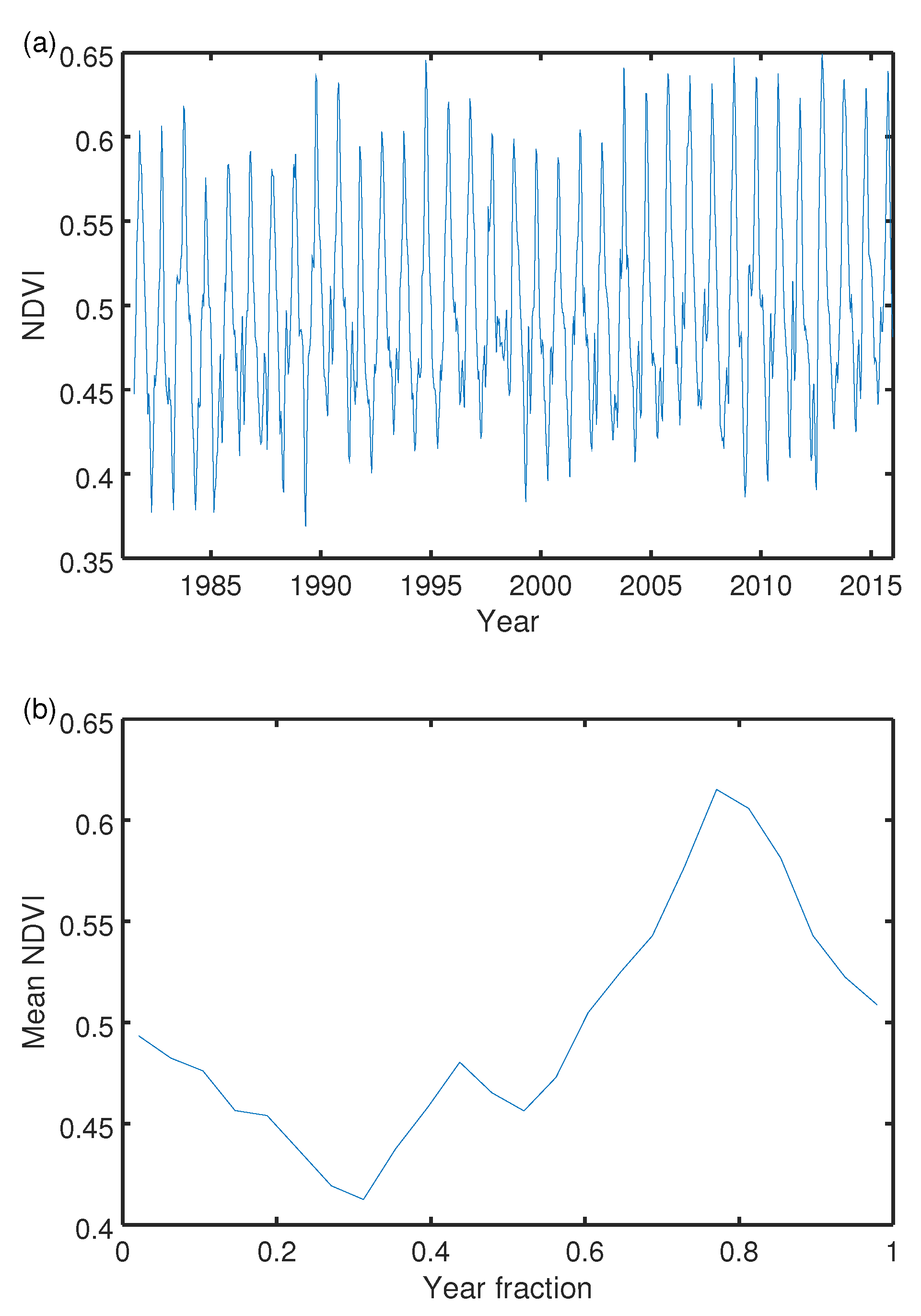
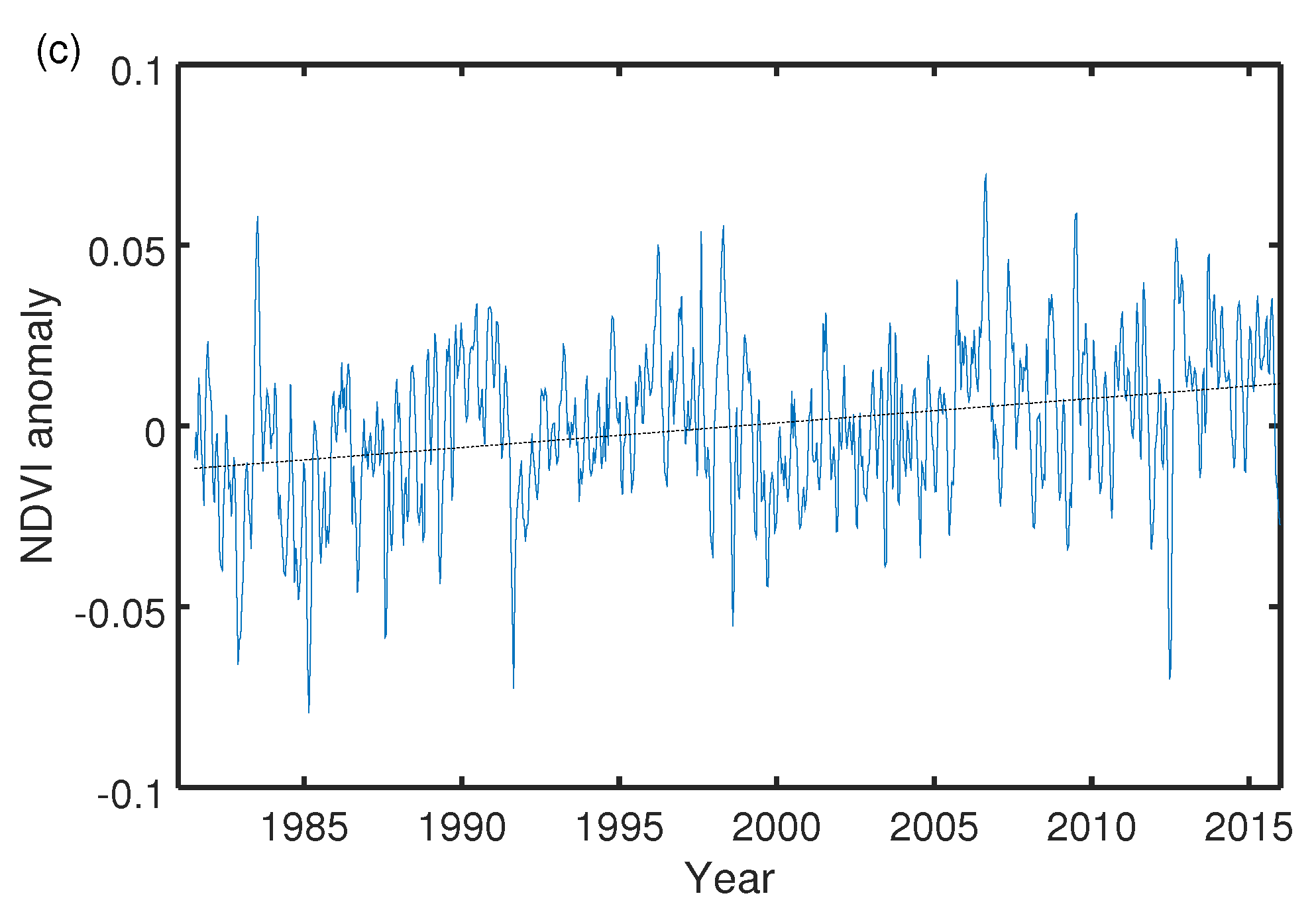
Figure 6.
(a) Mean normalized difference vegetation index (NDVI; unitless), and (b) 1981–2015 linear trend in NDVI (10 per year) for Nepal, by season and elevation.
Figure 6.
(a) Mean normalized difference vegetation index (NDVI; unitless), and (b) 1981–2015 linear trend in NDVI (10 per year) for Nepal, by season and elevation.

Figure 7.
The same as Figure 5, but using mean normalized difference vegetation index (NDVI) as predicted by the random forest regression model.
Figure 7.
The same as Figure 5, but using mean normalized difference vegetation index (NDVI) as predicted by the random forest regression model.

Figure 8.
Modeled 1981–2015 linear trend in normalized difference vegetation index (NDVI; 10 per year) for Nepal, by season and elevation, with (a) all forcings, (b) only CO-level change, (c) only land-use change, (d) only precipitation change, and (e) only temperature change.
Figure 8.
Modeled 1981–2015 linear trend in normalized difference vegetation index (NDVI; 10 per year) for Nepal, by season and elevation, with (a) all forcings, (b) only CO-level change, (c) only land-use change, (d) only precipitation change, and (e) only temperature change.

Table 1.
Area coverage (%) of Nepal by land cover category and year.
| Year | Forest | Shrub | Grass | Farm | Barren | Lake | Snow/Ice | Urban |
|---|---|---|---|---|---|---|---|---|
| 1990 | 45.2 | 2.2 | 11.7 | 25.3 | 6.8 | 0.6 | 7.9 | 0.2 |
| 2000 | 41.7 | 2.4 | 11.4 | 27.7 | 9.5 | 0.5 | 6.5 | 0.3 |
| 2010 | 42.1 | 2.3 | 10.5 | 27.3 | 8.6 | 0.5 | 8.4 | 0.4 |
Table 2.
Nash–Sutcliffe coefficients (NSC) and mean trend for random forest (RF) predictions of the normalized difference vegetation index (NDVI). The full RF model includes all time-varying factors. The other predictions are with either interannually constant factors or only one time-varying factor. The mean trend is in units per year. For comparison, the mean trend calculated from observations is per year.
| Trend | ||||
|---|---|---|---|---|
| Full RF | 0.959 | 0.288 | 0.793 | 0.422 |
| Constant | 0.941 | −0.000 | −0.068 | 0.000 |
| CO | 0.946 | 0.053 | 0.344 | 0.509 |
| Land cover | 0.945 | 0.034 | 0.238 | −0.135 |
| Precipitation | 0.946 | 0.102 | 0.043 | 0.020 |
| Temperature | 0.943 | 0.035 | 0.051 | 0.026 |
© 2017 by the authors. Licensee MDPI, Basel, Switzerland. This article is an open access article distributed under the terms and conditions of the Creative Commons Attribution (CC BY) license (http://creativecommons.org/licenses/by/4.0/).
Share and Cite
MDPI and ACS Style
Krakauer, N.Y.; Lakhankar, T.; Anadón, J.D. Mapping and Attributing Normalized Difference Vegetation Index Trends for Nepal. Remote Sens. 2017, 9, 986. https://doi.org/10.3390/rs9100986
AMA Style
Krakauer NY, Lakhankar T, Anadón JD. Mapping and Attributing Normalized Difference Vegetation Index Trends for Nepal. Remote Sensing. 2017; 9(10):986. https://doi.org/10.3390/rs9100986
Chicago/Turabian StyleKrakauer, Nir Y., Tarendra Lakhankar, and José D. Anadón. 2017. "Mapping and Attributing Normalized Difference Vegetation Index Trends for Nepal" Remote Sensing 9, no. 10: 986. https://doi.org/10.3390/rs9100986
Note that from the first issue of 2016, this journal uses article numbers instead of page numbers. See further details here.