Sensitivity of Landsat 8 Surface Temperature Estimates to Atmospheric Profile Data: A Study Using MODTRAN in Dryland Irrigated Systems


Water Desalination and Reuse Center, Division of Biological and Environmental Sciences and Engineering, King Abdullah University of Science and Technology (KAUST), Thuwal 23955-6900, Saudi Arabia
*
Author to whom correspondence should be addressed.
Remote Sens. 2017, 9(10), 988; https://doi.org/10.3390/rs9100988
Submission received: 15 June 2017
/
Revised: 8 September 2017
/
Accepted: 13 September 2017
/
Published: 23 September 2017
(This article belongs to the Special Issue Remote Sensing for Land Surface Temperature (LST) Estimation, Generation, and Analysis)
Abstract
:The land surface temperature (LST) represents a critical element in efforts to characterize global surface energy and water fluxes, as well as being an essential climate variable in its own right. Current satellite platforms provide a range of spatial and temporal resolution radiance data from which LST can be determined. One of the most complete records of data comes via the Landsat series of satellites, which provide a continuous sequence that extends back to 1982. However, for much of this time, Landsat thermal data were provided through a single broadband thermal channel, making surface temperature retrieval challenging. To fully exploit the valuable time-series of thermal information that is available from these satellites requires efforts to better describe and understand the accuracy of temperature retrievals. Here, we contribute to these efforts by examining the impact of atmospheric correction on the estimation of LST, using atmospheric profiles derived from a range of in-situ, reanalysis, and satellite data. Radiance data from the thermal infrared (TIR) sensor onboard Landsat 8 was converted to LST by using the MODTRAN version 5.2 radiative transfer model, allowing the production of an LST time series based upon 28 Landsat overpasses. LST retrievals were then evaluated against in-situ thermal measurements collected over an arid zone farmland comprising both bare soil and vegetated surface types. Atmospheric profiles derived from AIRS, MOD07, ECMWF, NCEP, and balloon-based radiosonde data were used to drive the MODTRAN simulations. In addition to examining the direct impact of using various profile data on LST retrievals, randomly distributed errors were introduced into a range of forcing variables to better understand retrieval uncertainty. Results indicated differences in LST of up to 1 K for perturbations in emissivity and profile measurements, with the analysis also highlighting the challenges in modeling aerosol optical depth (AOD) over arid lands and its impact on the TIR bands. Days with high AOD content (AOD > 0.5) in the evaluation study seem to consistently underestimate in-situ LSTs by 1–2 K, suggesting that MODTRAN is unable to accurately simulate the aerosol conditions for the TIR bands. Comparisons between available in-situ and Landsat 8 derived LST illustrate a range of seasonal and land surface dynamics and provide an assessment of retrieval accuracy throughout the nine-month long study period. In terms of the choice of atmospheric profile, when excluding the in-situ data, results show a mean absolute range of between 1.2 K to 1.8 K over bare soil and 3.3 K to 3.8 K over alfalfa for the different meteorological forcing, with the AIRS profile providing the best reproduction over the studied arid land irrigation region.
Keywords:
land surface temperature; Landsat; atmospheric correction; thermal infrared; remote sensing; AIRS; ECMWF; MOD07; NCEP; IGRA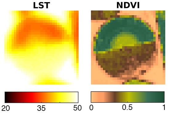
1. Introduction
Land surface temperature (LST) represents one of the key climate variables retrievable from space-based remote sensing platforms, offering insight into a range of environmental processes and linking multiple disciplines across the natural and physical sciences. Apart from being a fundamental variable in quantifying elements of the surface energy budget [1], LST has been used to study ocean–atmosphere interactions [2], to track global warming and climate change impacts [3,4], as well as being widely used in studies of vegetation monitoring [5], drought persistence [6] and urban climate assessments [7]. LST also plays a critical role in linking the water and energy cycles through its relationship with surface heat fluxes [8]. Indeed, thermal infrared (TIR) observations represent a fundamental element in efforts to map the spatial distribution of evaporation [9] as well as in efforts to constrain land surface model simulations [10]. Given the role that LST plays across broad aspects of earth and environmental sciences, determining its spatial and temporal variability is of considerable interest [11]. However, accurately determining its absolute value, in addition to describing its spatial and temporal development, is challenging given that LST varies considerably throughout the diurnal cycle as a function of the surface radiative balance, as well as expressing a broad range of spatial and temporal variations due to changing land surface and atmospheric conditions [12,13].
Thermal infrared observations from space offer the only plausible option for mapping LST over large areas, since in-situ measurements are unable to provide the density of coverage for adequate spatiotemporal information. A range of space-based thermal infrared platforms are available to retrieve the LST, including sensors onboard polar orbiting satellites such as the Moderate Resolution Imaging Spectroradiometer (MODIS) [14], the Visible Infrared Imaging Radiometer Suite (VIIRS), Gaofen 4, the Advanced Spaceborne Thermal Emission and Reflection Radiometer (ASTER), Sentinel-3, Landsat [15], as well as several geostationary platforms. The Landsat series of satellites offers one of the most complete and informative long-term records of surface temperature, providing a unique high spatial resolution (i.e., 60–120 m) thermal sequence that began with the launch of Landsat 4 in 1982 [16]. Although most of this extensive record only provides radiance data from a single infrared channel, the most recent addition to the Landsat fleet provides two longwave bands: Band 10 (10.60–11.19 µm) and Band 11 (11.50–12.51 µm), at a 100 m ground resolution and a 16 days temporal resolution.
Direct estimation of LST from thermal infrared measurements is a challenging task since the radiances measured by the satellites are influenced by both surface and atmospheric effects [17]. By using two TIR bands, atmospheric correction of the thermal data can be achieved using well developed split-window approaches [18] or temperature–emissivity separation techniques [19]. The split-window method, proposed by McMillin [20], was based on differential absorption across adjacent spectral windows and allowed for an estimate of sea surface temperature to be obtained by a linear combination of spectrally adjacent brightness temperatures. An adaptation of the McMillin [20] approach for application to land surfaces was presented by Becker and Li [18]. More recently, both Jimenez-Munoz et al. [21] and Rozenstein et al. [22] proposed split-window algorithms for the Landsat 8 thermal infrared sensor (TIRS). Using simulated thermal infrared data, the studies estimated mean errors of less than 1.5 K and 0.93 K, respectively. These methods were validated using simulated data from the Thermodynamic Initial Guess Retrieval and Standard Atmospheres included in MODTRAN code [23] and simulated radiance for a mid-latitude summer atmospheric profile with known LST and land surface emissivity (ε) [22]. The synthetic nature of these studies requires ongoing evaluation against in-situ measurements to further assess the performance of the LST algorithms over a range of land cover types and conditions. The temperature–emissivity separation (TES) approach of Gillespie et al. [19], developed for ASTER data, uses an iterative technique to remove reflected sky radiance. The TES algorithm hybridizes three established algorithms and estimates normalized emissivity first, while calculating emissivity band ratios afterward. Using simulated ASTER data, Gillespie et al. [19] recovered temperatures within ±1.5 K and emissivities within ±0.015. Wang et al. [15] used the same temperature–emissivity separation algorithm for Landsat 8, combining the two thermal bands with atmospheric profile data from the National Centers for Environmental Prediction (NCEP), and determined the average absolute error between their estimated LST and four surface radiation sites [24] to be 1.74 K, varying from 1.04 to 2.56 K.
The US Geological Survey (USGS) recently reported a calibration problem in the TIRS caused by stray light, resulting in a higher bias in one of its two bands (4% in Band 11, and 2% in Band 10) [25]. As such, relying on split-window algorithms for the estimation of LST from Landsat 8 becomes increasingly problematic, as the introduction of errors may prove difficult to quantify [26]. An alternative approach is to estimate LST using a single band or single-channel (SC) algorithm [27,28,29]. Three different single-channel methods are commonly found in the literature, including: (1) the radiative transfer equation (RTE) [27,28]; (2) the mono-window algorithm developed by Qin et al. [30]; and (3) the generalized single-channel (GSC) method developed by Jiménez-Muñoz and Sobrino [31]. These methods use the radiance measured by one of the Landsat TIRS bands and then correct the radiance using atmospheric profile data or total column water content. Atmospheric profiles can be obtained from ground-based atmospheric radio-soundings, satellite vertical sounders, or from meteorological forecasting models and reanalysis data. Unfortunately, ground-based radio-soundings are often difficult to obtain at the time of the satellite overpass and are sparsely recorded, making them suitable only for validation at specific sites [32]. To circumvent the spatial limitations of ground-based sounding data, atmospheric profiles derived from satellite platforms provide a large spatial extent, but can be compromised by relatively poor temporal resolution [28,33]. To overcome this spatiotemporal constraint, reanalysis data from weather prediction models provide a practical alternative to the spatial limitation of radio-soundings, while offering a flexible temporal resolution that can match retrieval requirements. Given the increasing availability of ground-based and reanalysis sources, a greater understanding of the limitations and uncertainties involved in using such data in LST retrieval schemes is required.
An example of a single-channel method that utilizes reanalysis data is a web-based correction tool proposed by Barsi et al. [34] that uses the NCEP modeled atmospheric global profiles as input to the MODTRAN radiative transfer model [23]. This procedure allows one to obtain the atmospheric transmission, upwelling radiance, and downwelling radiance values needed to convert sensor radiance into surface brightness temperature. McCarville et al. [35] expanded on this process by using the NCEP North American Regional Reanalysis (NARR) database as inputs. In a more recent study involving Landsat 8, Tardy et al. [36] evaluated MODTRAN using an automated Python tool that relies on the European Centre for Medium-Range Weather Forecasts (ECMWF) ERA-Interim product [37] as the source of atmospheric profile data. The authors evaluated the tool in southwestern France and central Tunisia by comparing the retrieved Landsat LSTs against in-situ LST measurements, resulting in an RMSE of 2.55 K for France and an RMSE of 1.8 K for Tunisia. These and related investigations have tended to examine the estimation of LST from Landsat using a single atmospheric profile source [31,36]. Importantly, relatively little attention has been paid to characterizing the sensitivity of LST to different atmospheric profile sources. Likewise, studies examining the atmospheric correction of Landsat 8 TIR imagery in arid lands are rather limited, despite the increased availability of cloud-free Landsat scenes in these environments that may help improve insights into spatiotemporal variability.
In addition to the source of atmospheric profile data, another potential source of uncertainty relates to the role that aerosols play in the prediction of LST. While the atmospheric correction in the thermal infrared is often focused on adequately accounting for the influences of water vapor and other trace gases [33], a key consideration in many regions of the world is the impact of aerosols and the role that dust plays in attenuating the satellite observed signal. The Saharan desert and its surrounds produce 50% of the mineral dust in the world [38], and dust is a recurrent feature throughout many arid and semi-arid environments [39]. While the impact of dust on the optical region of the electromagnetic spectrum has been well studied, understanding the role it plays on the thermal portion of the spectrum [38] and in dryland systems has not been examined as thoroughly [40]. Previous investigations have illustrated that even small increases in aerosol concentrations can significantly affect radiative fluxes [41]. A recent study focusing over the Red Sea and Arabian Peninsula estimated that the simulated domain average contribution of mineral dust to the total aerosol optical depth (AOD) was 87% [42]. Clearly, understanding the impact of the aerosol effect on retrieved surface temperature in such environments is an area of needed research and is one aspect explored herein.
The overall objective of this work focuses on the atmospheric correction of Landsat 8 thermal data over dryland systems [43], a climate zone that is relatively poorly represented in satellite-based temperature investigations, despite their importance in global energy budgets [44] and food production [43]. We explore this topic by characterizing the impact of using five different atmospheric profile records as input to MODTRAN. The atmospheric profile sources include satellite-based data from the Atmospheric Infrared Sounder (AIRS) onboard the Aqua satellite [45], as well as the Moderate Resolution Imaging Spectroradiometer Atmospheric Profile Product from the Terra platform (MOD07) [46], global reanalysis data from the ECMWF ERA-Interim [37] and the NCEP National Center for Atmospheric Research (NCAR) Reanalysis 1 [47], and in-situ balloon-based radiosonde releases from the Integrated Global Radiosonde Archive (IGRA) [48]. Furthermore, to evaluate the impact of input parameter errors on the atmospheric correction of Landsat 8 TIR data, a sensitivity analysis on the satellite and reanalysis atmospheric profiles was performed by applying randomly distributed errors into profile parameters such as temperature and relative humidity, as well as to ozone, CO2, and aerosol optical depth.
2. Materials and Methods
2.1. Study Site
The evaluation study was undertaken at the Tawdeehiya Arable Farm, which is located in the Al-Kharj region of Saudi Arabia, approximately 200 km southeast of Riyadh (Figure 1). The farm covers an area of around 70 square km and is comprised mostly of center-pivot irrigation fields producing crops that include alfalfa, carrot, Rhodes grass, barley, wheat, and maize. The region is largely cloud free for much of the year, providing an ideal environment to evaluate satellite data. Despite experiencing a predominance of cloud-free conditions, the farm is subject to occasional sandstorms that can influence measurements derived from remote sensors. Serendipitously, the site is located towards the edge of the Landsat 8 overpass, resulting in increased satellite coverage with a revisit time approaching 8 days (although missing the westernmost portion of the farm). The increased coverage results in a much greater density of usable imagery, which for this investigation includes 28 scenes collected during April to December 2015. Only Landsat scenes with a cloud cover metadata value below 30% were included in the study.
2.2. Ground-Based Land Surface Temperature Measurements
In situ LST measurements were obtained using two Apogee SI-111 infrared radiometers [49] that were connected to collocated meteorological stations, with the sensors recording high-frequency data that were averaged every minute. Two instruments provide long-term monitoring, with one placed inside an alfalfa field and the other over a bare desert soil. The radiometers cover an area of approximately 3 m2 and the spectral range of the Apogee sensors is 8 to 14 . The manufacturer reported accuracy of the instrument is 0.2 K from −20 to 65 °C when the target and detector temperature are within 20 K and 0.5 K from −40 to 80 °C when target and detector temperature differ by more than 20 K [49]. Surface temperature, together with meteorological measurements including air temperature, wind-speed, humidity, net-radiation and soil temperature, have been collected on a continuous basis since April 2015. The 2 m air temperature (used in Equation (1)) was collected from the weather stations using a Vaisala HUMICAP humidity and temperature probe (HMP155).
Determining an accurate LST can be achieved by removing the downwelling sky irradiance that is reflected into the sensor by the soil or canopy. If the sky temperature and surface emissivity are known, the surface temperature can be estimated following the Stefan-Boltzmann Law:
where (K) is the surface temperature, (K) is the surface temperature measured by the radiometer, (K) is the sky temperature, and ε is the surface emissivity [49]. Vegetation and bare soil emissivity values were assigned based on the ASTER Global Emissivity Dataset (GED) AG100 [50], which provides static emissivity information of all ASTER data acquired over a specific region for the period 2000–2008 at 100 m spatial resolution. The ASTER emissivity database is limited to this period due to failure of the ASTER SWIR detectors in 2008, resulting in cloud masking difficulties for the data beyond this period [50]. For the studied agricultural region, emissivity varies considerably between bare soil and vegetated areas. It is therefore important to distinguish between the different land cover pixels in an automated manner. Given that the Normalized Difference Vegetation Index (NDVI) has been demonstrated as an effective indicator of fractional vegetation in this particular environment [51], a simple NDVI threshold method was introduced to distinguish differences in the fractional vegetation coverage. The process identifies pixels with atmospherically- and adjacency-corrected Landsat 8 NDVI values [40] above 0.5, classifying these as full cover vegetation, while values below or equal to 0.2 were classified as bare soil. In the case of 0.2 ≤ NDVI ≤ 0.5, the pixel is composed of a mixture of bare soil and vegetation, and the emissivity is calculated as follows [29]:
where is the vegetation emissivity () and . is the soil emissivity (0.954). Vegetation emissivity was selected based on pixels with the highest NDVI (as provided by ASTER GED within the same product) in the alfalfa field, as this would be a more realistic value for a fully vegetated area than the exact location of the alfalfa radiometer. In contrast, soil emissivity was selected based on the location of the bare soil radiometer. The standard deviation of each particular emissivity value is 0.006 and 0.012 for alfalfa and bare soil respectively. is the vegetation proportion:
Emissivity changes from 0.973 to 0.954 following a quadratic function when NDVI is comprised in the range 0.2–0.5; otherwise, it remains constant (equal to and for alfalfa and bare soil, respectively). Sky temperature can be derived following Li et al. [52]. In their study, Li et al. [52] developed a comprehensive model for the estimation of the downward atmospheric longwave radiation for clear and cloudy sky conditions, with a relative root mean square error (rRMSE) of 2.77% for clear-sky conditions. The proposed model for daytime clear-sky conditions is a calibrated version from Brunt [53] and utilizes ambient temperature and partial pressure of water vapor as follows:
where is the sky temperature, is the ambient temperature, and is the partial pressure of water vapor. The partial pressure of water vapor can be expressed as a function of relative humidity (%) and ambient temperature (K) [54]:
Combined with the emissivity data, substitution of Equation (4) into Equation (1) allows one to obtain the LST ().
2.3. Satellite Based Thermal Infrared Data
As noted earlier, due to known calibration problems in the dual thermal bands of Landsat 8 [25], we explore the estimation of LST from using the single-channel method [27,28]. This method uses the radiance determined from Band 10 onboard the Landsat 8 TIR scanner and corrects the radiance for residual atmospheric attenuation and emission using atmospheric profile data. The atmospheric profiles for this particular study are derived from AIRS, MOD07, NCEP-NCAR Reanalysis 1, and ECMWF ERA-Interim: further details of which are provided in Section 2.4. The technique requires a priori knowledge of the pixel emissivity in the TIR channel, which were acquired from the ASTER Global Emissivity Dataset (GED) AG100 [50] as described in Section 2.2.
Landsat 8 data were retrieved as Level 1 (L1T) (version LPGS 2.5.1) data products. The L1 product consists of quantized and calibrated scaled digital numbers (DN) representing image data. A conversion to top of atmosphere (TOA) radiance is achieved through use of:
where is the TOA spectral radiance , is the band-specific multiplicative rescaling factor from the metadata (RADIANCE_MULT_BAND_X, where X is the band number), is the band-specific additive rescaling factor from the metadata (RADIANCE_ADD_ BAND_X, where X is the band number), and is the quantized and calibrated standard product pixel values (DN) [55]. The TIRS band data are converted to brightness temperature using the following:
where is the satellite brightness temperature (in Kelvin), and and [K] are the band-specific thermal conversion constant from the metadata (K1_CONSTANT_BAND_X and K2_CONSTANT_BAND_X, where X is the band number).
Although the Landsat TIR data are sensed at a 100 m resolution, a cubic resampling to 30 m pixel resolution is provided. The full swath Landsat data were subset to an 800 × 800 pixel region covering the Tawdeehiya farm. In deriving surface temperature, the atmospheric profile geographically closest to the weather stations was selected for each unique Landsat 8 scene. However, the closest profile is not always the most representative of the region, so errors in the real-time composition of the atmosphere are to be expected. This becomes a pertinent issue when using MOD07 profiles since the frequency of observations gradually declines towards the Equator.
2.4. Satellite Based Meteorological Data
Meteorological data sensed by satellites can provide the geopotential height, temperature, and relative humidity parameters that are needed for the atmospheric correction of TIR data. Ozone and CO2 are also measurable through multispectral platforms, such as MODIS, and provide further details into the composition of the atmosphere at the time of Landsat 8 overpasses. In addition to these parameters, information on aerosols is available in the form of aerosol optical depth, which can also be used in the atmospheric correction of TIR data. The various needed parameters and their respective sources are briefly described below, with additional information provided in the associated references.
Atmospheric Infrared Sounder (AIRS): The AIRS instrument onboard the Aqua satellite is designed to measure atmospheric water vapor and temperature profiles on a global scale [45]. The high-resolution spectrometer has 2378 bands in the thermal infrared (3.7 to 15.4 ) and 4 bands in the visible, with a 45 km spatial resolution. The AIRS L3 atmospheric profile product has a temporal difference of three hours with the Landsat 8 satellite overpass time, with Landsat 8 covering the Tawdeehiya farm at approximately 10:10 and AIRS at 13:30 local time. Retrieved air temperature and geopotential height are provided at 28 standard pressure levels, from the surface to 10 Pa. The temperature profile product is provided at an accuracy of 1 K per 1 km thick layer in the troposphere, while the moisture profile product has a reported accuracy of 15% per 2 km thick layer in the lower troposphere (20–60% in the upper troposphere) [56]. Geopotential height, temperature, and relative humidity were obtained from this platform and used for the atmospheric correction of Landsat 8 TIR imagery. In addition to water vapor and temperature, AIRS also provides a CO2 product that is required for the atmospheric correction of TIR imagery: the AIRS mid-tropospheric Carbon Dioxide (CO2) Level 3 Daily Gridded Retrieval, with values presented in a 2.5° × 2° global grid and with units of mole fraction (106 × data = ppm in volume). A study by Chahine et al. [57] found that a comparison between the AIRS retrieved CO2 mixing ratio and Matsueda [58] flask measurements results in a bias (Matsueda-AIRS) of 1.15 ppmv, with a standard deviation of ±3.1 ppmv. The AIRS mid-tropospheric CO2 product also provides standard deviations and standard retrieval means.
MODIS atmospheric profiles product: The MOD07 product onboard Terra provides information on total-ozone burden, temperature and moisture profiles, as well as atmospheric water vapor [46]. These parameters are produced day and night at a 5 km pixel resolution. The MOD07 L2 atmospheric profile product has the benefit of a near temporal coincidence with the Landsat 8 satellite overpass time. MOD07 uses 11 infrared MODIS bands (25, and 27–36) providing atmospheric parameters at 20 pressure levels. Sobrino et al. [59] compared MOD07 to radiosonde data over the Iberian Peninsula and found that values extracted from daytime water vapor show a bias of 0.3 ± 0.5 cm, with an RMSE of 0.55 cm. The authors also found the air temperature profiles from MOD07 to have an RMSE of around 3.6 K on average. Geopotential height, temperature, and relative humidity were obtained from MOD07 and used in the atmospheric correction.
MODIS aerosol product: The MODIS Gridded Atmospheric Product (MOD08, Collection 6) provides information on aerosols at a daily scale [60]. MOD08 contains statistics derived from several science parameters from the Level 2 Atmosphere products, with values presented in a 1° × 1° global grid. The MOD08 product reports aggregated information on aerosols retrieved from the MODIS Aerosol Product (MOD04) that employs the MODIS Deep Blue algorithm for the estimation of aerosol optical depth over bright land areas [61]. Hsu et al. [61] found that the AOD values from the Deep Blue algorithm were generally within 20–30% of those measured by sun-photometers. Furthermore, Sayer et al. [62] found the expected error (EE) for the algorithm to be over land when comparing the MODIS Collection 6 product to 60 Aerosol Robotic Network(AERONET) validation sites.
2.5. Reanalysis Based Meteorological Data
To obtain the necessary fields of geopotential height, temperature and relative humidity needed for atmospheric correction, and to test the sensitivity of the retrieval algorithms to different forcing data sources, a range of reanalysis products were also employed in parallel to the atmospheric profiles determined from satellite observations. These are described briefly below, with additional information provided in the listed references.
NCEP/NCAR Reanalysis 1: NCEP/NCAR Reanalysis 1 [47] dataset contains atmospheric profile information from 1948 to present-day and has a 6-h daily temporal coverage (0:00, 06:00, 12:00, and 18:00 UTC) with a 2.5° by 2.5° spatial resolution. The data assimilation scheme is a three-dimensional variational (3D-VAR) that produces global fields of geopotential height, temperature and relative humidity. These parameters are mostly provided across 17 pressure levels [63], while the relative humidity is provided at 8 pressure levels (to 300 ).
ECMWF ERA-Interim: The ECMWF European Reanalysis (ERA) Interim product [37] is a global atmospheric reanalysis covering the period from January 1979 to present. The data assimilation system to produce this dataset is based on a 2006 release of the IFS (Cy31r2) and includes a four-dimensional variational analysis (4D-Var) with a 12-h analysis window. The spatial resolution of the ERA-Interim dataset is approximately 80 km and consists of 6-hourly atmospheric fields across 60 vertical model levels, providing pressure, potential temperature and potential vorticity from the surface up to 0.1 .
2.6. Radiosonde Meteorological Data
In addition to the satellite and reanalysis based atmospheric profiles, radiosonde data from the Integrated Global Radiosonde Archive (IGRA) were utilized in our investigation. IGRA consists of balloon-based radiosonde observations that have been released from over 2700 global stations. The closest station to our study site is located near the city of Riyadh, at the King Khaled International Airport (station SAM00040437, with a latitude and longitude of 24.93 and 46.72). The data from this site provide twice-daily (around noon and midnight) relative humidity and temperature products from 1984 onwards, including up to 40 pressure levels (1000 to 10) and can serve as a benchmark against which to compare the satellite and reanalysis profiles. The radiosonde data from noontime releases are used in our analyses in order to consider the closest time to Landsat 8 overpass.
2.7. Atmospheric Correction Using MODTRAN
Although there are a number of radiative transfer models available for atmospheric correction that have been proposed and reviewed in the literature, such as SMAC [64], 6S [65] and ATCOR [66], the present study explores the application of the widely employed MODTRAN model [23]. MODTRAN is an atmospheric radiative transfer model that has been employed in a wide variety of remote sensing applications, including the atmospheric correction of TIR satellite data [29] as well as thermal and narrowband multispectral data from unmanned aerial vehicles [67]. The radiative transfer model is controlled by an input file, known as “tape 5” or “rootname.tp 5”, which consists of a sequence of six or more formatted input lines detailing variables and flags necessary for its operation. In addition to employing a range of standard atmospheric profiles for radiative transfer estimation, the user has the option to modify or supplement vertical profiles for temperature, pressure, and default molecular gases such as O3 and CO2 (amongst others). In addition to this, the variable IHAZE in the code specifies the aerosol model used for the boundary-layer (0 to 2 km), chosen to be DESERT (IHAZE = 10) for this study. Furthermore, default aerosol options specified by IHAZE can also be modified or supplemented by the user in the form of meteorological visibility range (VIS) or through definition of the 550 nm AOD. Atmospheric vertical profiles from both satellite-based MOD07 and AIRS products and reanalysis derived NCEP/NCAR and ECMWF datasets were introduced into MODTRAN. However, defining atmospheric profiles in the MODTRAN code limits the atmospheric modeling to the available data. AOD values at 550 nm were extracted from the MOD08 product and used in the main aerosol component of MODTRAN to evaluate their influence on the LST results.
By modeling the atmosphere with MODTRAN, the radiances emitted by the surface of the Earth can be estimated if the radiances at the sensor (satellite) are known. The sensor radiance can be expressed as [68]:
where is the surface emissivity at wavelength , is the spectral radiance from a blackbody at surface temperature T, is the spectral radiance incident upon the surface from the atmosphere (calculated from MODTRAN), is the spectral radiance emitted by the atmosphere (from MODTRAN), is the spectral atmospheric transmission (also from MODTRAN), and is the spectral radiance observed by the sensor.
If band emissivity is known, it is possible to correct for the downwelling sky radiation in Equation (8) and the surface temperature can be calculated by inversion of Planck’s Law [28]:
where is the surface temperature in Kelvin, is the band radiance (from Equation (8), ), and and are calibration constants chosen to optimize the approximation for the band pass of the sensor ( and for Landsat 8).
2.8. Description of Evaluation Statistics
A number of standard statistical metrics were used in the evaluation of satellite-based LST retrievals using in-situ estimates. These include:
Mean Absolute Error: Mean Absolute Error (MAE) is defined as follows:
where is a prediction, is an observation, and n is the number of observations. In other words, the MAE is the average of the absolute difference between the predictions and the observations.
Mean Error: Similar to MAE, the mean error (ME) (or bias) is the average of all errors, with the exception that the errors () are not absolute. ME is defined as follows:
The mean error is useful in determining if a model is underestimating () or overestimating () the observed variables.
Root-mean Squared Error: The Root-mean Squared Error (RMSE) is defined as follows:
Coefficient of determination: The coefficient of determination (R2) is defined as follows:
where represents the dataset, the mean, and the modeled value. In this study, the modeled values are obtained by a linear regression of the form , where m and b are calculated by ordinary least-squares regression.
3. Results
Landsat-based LST were discriminated into four different categories, relating to the source of the profile data used for the atmospheric correction i.e., MOD07, AIRS, NCEP, and ECMWF driven LST retrievals. Radiosonde data were used in the bare soil and alfalfa analyses to both evaluate the satellite and reanalysis profile data and to compare the derived LST products against the in-situ measurements. In addition to Landsat-based temperature comparisons against the in-situ data (Section 3.1), the sensitivity of MODTRAN to relative humidity, temperature, emissivity, CO2, ozone, and AOD (Section 3.2) was also evaluated by introducing randomly distributed errors into the atmospheric variables. Applying these uncertainties to the satellite and reanalysis atmospheric parameters, with errors introduced into one atmospheric input variable while others were kept constant, allows a perturbation experiment to be undertaken.
3.1. Evaluation against In-Situ Observations
Evaluation of TIR imagery was performed by comparison against the in-situ data installed at both the alfalfa (Figure 2) and bare soil desert sites over the period April to December 2015. Multiple Landsat 8 data were compiled, with a total of 28 images for bare soil analysis selected for this period, and a total of 23 images for alfalfa selected for the period June to December. The differing periods correspond to the start of operations of the weather stations over the different land cover types. As this is a working agricultural farm, the alfalfa field is subject to periodic harvesting. Unfortunately, to reduce potential damage to the instrument during harvesting, the area over which the infrared radiometer senses is not routinely trimmed, resulting in a potential land cover related bias relative to the rest of the field. As such, only radiometer data that provide a representative measurement (i.e., when the field is well covered in vegetation) are used in the analysis.
For the atmospheric correction of the Landsat 8 TIR imagery, atmospheric profile data from the four different sources were ingested into MODTRAN. A single LST pixel corresponding to the location of the in-situ measurements was extracted from the imagery for each of the distinct Landsat 8 profile records and compared against the in-situ measurements at a time coincident with the Landsat 8 overpass. LST from in-situ locations was calculated following Equations (1) and (4) (see Section 2.2), making use of air temperature and humidity that was collected by the weather stations collocated with the radiometer data, as well as emissivity data following Equation (2).
Figure 3 and Figure 4 illustrate the differences between the Landsat-based LST estimates and in-situ LST for each of the studied land covers. The Landsat-coincident in-situ LST record is also shown for reference (Figure 3a and Figure 4a). Examining the bare soil response (Figure 3a), the in-situ LST shows a temperature variation of over 20 K during the study period at the time of the Landsat overpass. The highest recorded temperature at the time of Landsat overpass is 56.2 °C, while the lowest recorded temperature is 28.2 °C. LST over bare soil in the summer days varies considerably within the same day, showing a diurnal temperature range of over 40 K in some instances. For example, the highest recorded in-situ temperature for DOY217 is 64.4 °C, while the lowest (for the same day) recorded temperature is 21.5 °C. As expected, bare soil LST during the December winter period has a lower variability during the same day. For DOY352, the highest recorded in-situ temperature is 33.2 °C, while the lowest recorded temperature for the same day is 7.4 °C. In other words, the in-situ LST diurnal difference during the summer is almost twice of that during the winter over bare soil.
LST calculated from all the atmospheric profile sources (ECMWF, NCEP, AIRS, and MOD07) over bare soil generally underestimates (Figure 3) the in-situ LST in the period from April to June (subsequently referred to as the spring period), while mostly overestimating the in-situ LST for the rest of the study period. Interestingly, the spring period has a larger AOD than other periods of the year, except for DOY153. It is important to note that during the spring period, calculated LST from all the profile sources for DOY153 (with an AOD of 0.21) are overestimated. The analysis from the spring period suggests that MODTRAN is not accurately correcting for the influence of AOD in the satellite signal. The effect of AOD on LST can be seen again on DOY297, where an increase in AOD (AOD = 0.78) corresponds to an underestimation of calculated LST from all the profile sources. Although there is a predominant trend, there are a few instances (DOY 105 and 288) where this is not reflected. Further analysis on the influence of perturbing AOD and its influence on LST will be presented in Section 3.2.
Overall, the LST calculated from the AIRS atmospheric profile product (AIRS LST), with an of 0.97 and a MAE of 1.19 K (Table 1), indicates the best performance for the bare soil analysis. The AIRS LST result also compares to the NCEP based LST result from our study, with an of 0.96 and a MAE of 1.25 K. Similarly, the ECMWF LST has an of 0.96 for bare soil, albeit with a larger MAE of 1.44 K when compared to the NCEP LST, respectively. These values are consistent with the work of Tardy et al. [36], who undertook an analysis in a comparable arid land environment using ECMWF atmospheric profiles as input to MODTRAN. Here, the RMSE from the ECMWF LST for the Tawdeehiya based example is 0.26 K lower (Table 1) than the Tardy et al. results, based upon a similar number of data points over undisturbed soil (38 days in Tunisia versus 28 days in Saudi Arabia).
The MOD07-based bare soil LST performed the poorest with an of 0.94 and a MAE of 1.77 K. The MOD07 result was somewhat surprising given the similar sensor observation time to Landsat, as well as having the highest spatial resolution among all the profile sources (Section 2.4). Further analysis of the MOD07 atmospheric profile indicated that the coverage of the MODIS Terra satellite over the farm at the dates of Landsat overpasses is located mostly at the edge of the swath, with a viewing angle ranging from 10° to 60°, which may impact upon retrievals. In contrast, the viewing angle of the MODIS Aqua satellite (upon which AIRS is installed) is associated with comparatively lower values during the same conditions than the MODIS Terra satellite. In addition to a more suitable viewing angle, the hyperspectral sensing capabilities of AIRS make it a potentially better Earth-observing platform than MODIS over the study region. This justifies the improved performance of this dataset with respect to other profiles.
For the alfalfa field response (Figure 4), the temperature variation during the same period is approximately half (11.8 K) of that over the bare soil, with the highest recorded temperature having a value of 34.4 °C and the lowest recorded temperature a value of 22.6 °C. In-situ LST over alfalfa in the summer shows a diurnal temperature variation of approximately 20 K: half of that over bare soil. For example, using the same day as the previous example over bare soil, the highest recorded in-situ temperature over alfalfa is 37 °C (64.4 °C over bare soil), while the lowest temperature is 17.5 °C (21.5 °C over bare soil). Contrary to the bare soil example, LST over alfalfa in the winter days has a similar diurnal variability to that of the summer days. Following the previous example over bare soil, in-situ LST during the same day ranges from 7.1 to 25.5 K. This result is not surprising, since, although land surface temperature is expected to change abruptly in arid lands, plants are able to regulate their temperature throughout the year via transpiration, reducing the amplitude of the alfalfa response.
Landsat-based LST estimates over alfalfa (Figure 4) illustrate a positive bias relative to the in-situ measurements for all the atmospheric profile sources. There are a number of anomalously large differences that can be seen between in-situ measurements and all of the Landsat-based profile estimates throughout the study period. These large differences correspond to periods shortly after crop harvesting, as indicated by the NDVI provided in Figure 4a. In these instances, the satellite-based estimates can measure 8–14 K higher (Figure 4) than the corresponding in-situ radiometer measurement. To avoid introducing these spurious events, a temporal filter based on the NDVI was implemented to ignore days when the radiometer is unable to provide a representative measurement. Pixels with atmospherically- and adjacency-corrected NDVI values [40] greater than 0.3 were considered as fully vegetated, while pixels not fulfilling these conditions were ignored. After having discarded such instances, the total number of available scenes for alfalfa was reduced to 17. Statistics for both data sets (filtered vs. original) are provided (Table 1).
The LST calculated from the NCEP atmospheric profile product shows a coefficient of determination of 0.93 and a mean absolute error of 3.31 K (Table 1), providing the best performance for the alfalfa analysis. There are a number of possible explanations for the high uncertainties over the alfalfa canopy. On one hand, the emissivity estimated from the ASTER Global Emissivity Dataset might be more suitable as a first guess over homogeneous land covers, such as bare soil, than over heterogeneous land covers, such as vegetation. Moreover, emissivities from the ASTER GED are within ±0.015 [19], which could result in larger errors in the estimation of LST. On the other hand, the Apogee radiometer over the alfalfa field is located near the center of the pivot, meaning that Landsat is observing a mixed signal from the bare soil in the center and the surrounding alfalfa (Figure 2). The mixed response is apparent in the positive bias (Table 1 and Figure 4) of the alfalfa analysis. McCabe et al. [69] studied the subpixel temperature variability and found it to exceed 1 K in the 8–12 band with a subpixel temperature difference of 30 K. A temperature difference of 30 K between vegetation and bare soil is certainly possible in these arid environments (Figure 3a and Figure 4a). Furthermore, differences in the emissivity between the soil and the alfalfa are also contributing to the temperature bias. In the same study, McCabe et al. [69] found that for a 50:50 material mixture at the same temperature, changes in emissivity of 0.02 (from 0.98 to 0.96) produce a temperature difference of approximately 0.4 K in the 8–12 band.
In visits to the Tawdeehiya farm during the study period, the plants in the immediate vicinity of the radiometer indicated signs of insect or fungal infestation. The potential land cover related bias relative to the rest of the field might have affected the in-situ LST measurements in a way such that the in-situ measurements are not entirely representative of the alfalfa field as seen from Landsat. These, together with other potential sources of error including atmospheric profile data, are examined in the following section.
In addition to the four atmospheric profile sources, radiosonde data [48] were ingested into MODTRAN to calculate LST over bare soil. However, the number of available Landsat scenes is reduced to 24 as per the availability of the radiosonde data. Figure 3f and Figure 4f show the calculated LST for the same time period as previously described. The LST derived from balloon-radiosonde shows a similar coefficient of determination to AIRS (0.96), albeit with a smaller MAE of 1.11 K (1.18 K for AIRS) for the 24 Landsat scenes over soil. Despite being around 200 km away from the Tawdeehiya farm, the LST derived from the radiosonde site performs well over bare soil. The difference in LST (Landsat minus in-situ) generally decreases when using the radiosonde profile, although the LST calculation has issues on the same days as the LST calculated from the other profile sources (i.e., DOY 153, 224, and 240). Interestingly, the radiosonde-based LST for alfalfa performs poorly when compared to the rest of the profiles (Table 1). Upon close inspection, it can be seen from Figure 4 that the missing radiosonde days correspond to data with a lower LST difference, which results in an overall higher MAE when these are not considered.
3.2. The Role of Variability in Atmospheric Profiles
The sensitivity of MODTRAN to discrepancies in the atmospheric profiles was analyzed by introducing normally distributed errors into the relative humidity (RH), air temperature (T), carbon dioxide (CO2) and ozone (O3). The form of the introduced errors follows a normal (or Gaussian) distribution with mean (µ) 1 and variance (σ) 0.1 and is multiplied by the error. Similarly, a negative error is also studied with µ = −1 and σ = 0.1. For example, the introduced perturbation for a 15% error is comprised of a normally distributed number (µ = ±1, σ = 0.1) that is multiplied by the error range (in this case 15%). For this example, and given that 95% of values in a normal distribution are found within ±2σ, the additive or subtractive error could be anywhere from ±12% to ±18% but predominantly around ±15%. This is done for each profile at each measurement height, and seeks to replicate the introduction of uncertainty into the atmospheric profile measurements to study sensitivity in LST retrievals. Contrary to uniformly distributed errors [70] and fixed errors [21] introduced to atmospheric profiles when assessing sensitivity, a normally distributed perturbation provides a behavior commonly found in nature [71].
The 15% error introduced to the RH profiles is chosen following the previously reported accuracy of the RH in the AIRS atmospheric profiles products (Section 2.4). Similarly, an error around ±1 K was introduced to all the temperature profiles as a first guess, also following the reported accuracy of T in the AIRS atmospheric profiles products. An example of the RH and T profiles from AIRS, ECMWF, NCEP, MOD07, and radiosonde for DOY 105, 240, and 288 is shown in Figure 5. The radiosonde profiles, despite being 200 km away from the farm, appear to be adequately represented by the AIRS and ECMWF profiles. Differences between the MOD07 and radiosonde profiles are evident, particularly in DOY 288 (Figure 5c). MODTRAN sensitivity to aerosol optical depth at 0.55 in the TIR region was also analyzed following the expected error in the MODIS Deep Blue algorithm [61] (Section 2.4) for the highest quality retrievals over land. The impact of error in emissivity was also studied by introducing an error around ±0.01 (ε ranges from 0 to 1). Percentage errors in the range from ±5 to ±20% were examined across each of the variables. The impact of the errors of ±5%, ±10%, ±15% and ±20% were introduced into all the atmospheric profile sources for the year 2015 and detailed below. Since the impact of variations in O3 and CO2 resulted in minimal variation in LST (below 0.01 K and 0.1 K, respectively), these are not discussed in further detail.
3.2.1. Relative Humidity
Relative humidity is an important parameter in the calculation of satellite-based LST, as small changes in water content accuracy, due to the absorption of TIR radiation by water vapor [31], can result in large LST deviations. As can be seen from Figure 6, an error of 15% in relative humidity (RH15) over bare soil produces a mean difference of 0.19 K in the ECMWF LST, 0.37 K for the NCEP LST, 0.39 K for the AIRS LST, and 0.32 K for the MOD07 LST (Figure 6a–d, respectively). Interestingly, an RH15 over alfalfa produces a mean difference of roughly half of that for soil (0.11 K) for the ECMWF profile, 0.22 K for the NCEP profile, 0.22 K for the AIRS profile, and 0.19 K for the MOD07 profile (Figure 6e–h). Figure 7 shows the influence of the errors (RH05, RH10, RH15, and RH20) in Landsat-based LST for all the atmospheric profile sources over bare soil, while Figure 8 depicts the influence of the errors over alfalfa. A consistent increase in the LST error is seen both over soil and alfalfa when introducing errors in relative humidity, albeit having a smaller influence over alfalfa. Differences in LST are up to 1.5 K (Figure 7) when an error of 20% is introduced (RH20) over bare soil and over 1 K over alfalfa (Figure 8).
An error of 20% (RH20) is not unusual in the retrieval of satellite-based relative humidity, reaching 7–27% near the land surface for AIRS [56]. Accuracy in the retrievals of relative humidity for the estimation of LST are particularly important near the boundary layer, as a larger amount of water vapor is present in this zone than in the upper layer. Moreover, the coarse spatial resolution of satellite platforms may not discriminate the water vapor signal at the spatial resolution of irrigated farms and could be a source of further uncertainties in these and the reanalysis data (since they also ingest satellite data). The different LST results for soil and alfalfa suggest that changes in the atmospheric composition in regard to relative humidity have a weaker effect over the vegetated areas due to the overall lower energy emission by the vegetated land cover when compared to the bare soil, i.e., LST over alfalfa is consistently 20 K to 30 K cooler than bare soil (Figure 3 and Figure 4).
3.2.2. Emissivity
Emissivity is a critical variable in the estimation of LST, since the energy emitted from the surface in the TIR region is a function of emissivity (Equation (8)). As can be seen in Figure 6, an error of 0.01 in emissivity (e10) over bare soil produces a mean difference of 0.74 K in the LST calculated from the ECMWF profile, 0.70 K for the NCEP profile, 0.71 K for the AIRS profile, and 0.74 K for the MOD07 profile (Figure 6a–d). Contrary to the RH case, the LST differences due to discrepancies in emissivity do not follow the same pattern. An error of 0.01 in the ECMWF profile over alfalfa produces a mean difference of 0.67 K, while the NCEP results in a mean difference of 0.64 K (Figure 6e,f). In addition, similar errors in the AIRS profile produce an LST mean difference of 0.66 K and the MOD07 profile produce an LST difference of 0.69 K for the same 0.01 error (Figure 6g,h). Errors of 0.005, 0.15, and 0.20 (e05, e15, and e20) were also introduced into the LST calculations for all the atmospheric profiles. As can be seen in Figure 7, discrepancies in emissivity have a stronger influence on the LST than the rest of the parameters, including RH. An emissivity error of 0.01 is not unusual and actually below the ±0.015 range that the ASTER GED product is expected to provide [19]. Having used an annual average value for emissivity for bare soil and alfalfa, it would be reasonable to expect errors in Landsat-based LST to exceed 1 K (errors of 0.01–0.02 in emissivity) using the single-channel method and ASTER GED emissivity.
3.2.3. Temperature
Temperature profiles are also an essential variable in the atmospheric correction of TIR imagery, as water vapor content is calculated in the RTE from RH using temperature profile data. Randomly distributed errors of 0.5 K, 1 K, 1.5 K and 2 K (T05, T10, T15, and T20) in the air temperature were introduced into all the atmospheric profile sources. However, errors introduced to the temperature profile have a smaller effect than those to the relative humidity and emissivity (Figure 6), having a mean error ranging from 0.06 K to 0.1 K for soil and almost zero (0.05 K to 0.08 K) for alfalfa. Temperature profile accuracy appears to have an effect on Landsat-based LST when it exceeds 2 K, as differences in satellite-sensed LST can reach values as high as 0.7 K over bare soil (Figure 7). Similar to the RH case, the effect of the lower energy emission by the vegetated land cover (when compared to the bare soil) is apparent in the temperature perturbation (Figure 7 and Figure 8).
3.2.4. AOD
The effect of varying aerosol loadings is often ignored (i.e., defined as an atmosphere with a constant visibility) in the atmospheric correction of TIR imagery [28,29,31,36], despite evidence of dust affecting the satellite signal [72]. For arid land agricultural systems, the potential increases in dust loadings [73] constitutes a valid concern on characterizing such influences. Other agricultural regions in the world might be able to escape the need for quantifying the effects of AOD in the LST calculations, as the AOD values are generally lower than over arid lands throughout the year [74]. Overall, LST values calculated using all the atmospheric profile sources were less affected by the introduction of errors to AOD than some other variables. The expected error for the MODIS Deep Blue algorithm [61] (Section 2.4) produced an LST difference below 0.25 K (Figure 6). However, studies have found that the discrepancies between the Deep Blue algorithm and ground truth are somewhat larger over bright desert surfaces than over other land cover types [75], suggesting that errors in AOD could be larger in arid lands. Following this, larger variations to those suggested by Kahn et al. [76] and Sayer et al. [62] were introduced into the calculations. The larger variations in AOD did not result in large LST errors, being below 0.5 K for AOD errors of up to 40% (Figure 6 and Figure 7): potentially far from the actual expected errors of AOD from the MODIS Deep Blue algorithm over arid lands. Furthermore, the results from Section 3.1 (Figure 3) suggest that MODTRAN might not be properly correcting for the effect of aerosols on high AOD days, as LST from days with a high AOD are mostly underestimating the in-situ radiometer measurements.
4. Discussion
The work presented here contributes to the atmospheric correction of Landsat 8 in arid lands, a climate zone that is relatively poorly represented in satellite-based temperature investigations. The increased availability of cloud-free Landsat scenes in these environments provides a rich dataset that helps to improve insights into spatiotemporal variability. Results indicate that the major physical parameters controlling the accuracy of the satellite retrieved LST include the relative humidity and emissivity. An introduced uncertainty of 20% in relative humidity can result in LST errors as high as 1.5 K for bare soil and 1 K over alfalfa in irrigated arid environments, while an uncertainty in emissivity values of 0.01 can result in errors between 0.7 and 1 K for both land cover types. Typically, determining the emissivity with any degree of precision is a challenging task, so an error of 0.01 in emissivity is certainly not unusual and in line with the reported standard deviation in the emissivity values taken from the ASTER GED. Ozone and CO2 were found to have much smaller influences on the estimated LST for all the atmospheric profiles and were not seen to significantly affect the results relative to the other sources of error.
The AIRS profiles generally better performance over bare soil might be attributed to its capacity to represent the local atmospheric conditions better than reanalysis sources. Figure 5 suggests that the AIRS and ECMWF are consistent with the available radiosonde record. In contrast, MOD07 seems to be unable to accurately represent the conditions sensed by the radiosonde. This is particularly evident in DOY 288 (Figure 5c), where MOD07 has serious discrepancies compared to the rest of the profiles. Landsat-based LST from the MOD07 profile was expected to provide better results, as the overpass time is within 30 min of that from Landsat. However, it was discovered that the MOD07 profile is located at the edge of the swath, affecting the quality of the data. Moreover, contrary to AIRS, MOD07 is not a sounding instrument and its precision might be lower than that of AIRS for the same conditions in the region.
Aerosol optical depth is of interest in arid lands since dust sources, regardless of size or strength, can usually be associated with topographical lows located in these regions [77]. Furthermore, aerosols covering large areas in the region affect the satellite signal [72], and AOD variability is seldom considered in the estimation of LST [28,29,31,36]. Recent studies have found that the discrepancies between the Deep Blue algorithm and ground truth are somewhat larger over bright desert surfaces than over other land cover types [75]. In particular, over arid sites and across 16 AERONET validation sites, 37% of the studied points fall outside of the reported error for the Deep Blue algorithm [62]. The arid sites region includes the “Solar Village”, located approximately 200 km northwest of the Tawdeehiya farm. The Deep Blue algorithm for this site has an RMSE of 0.16, larger than the average of 0.145 for all the arid sites [62]. In addition, 40% of the studied points fall outside of the reported error, suggesting that the AOD errors in this region could be larger.
The effect of AOD in the satellite signal is apparent in the Landsat-based LST validation of the atmospheric correction results, where LST from days with a high AOD were mostly underestimating the radiometer measurements (Figure 3). While not necessarily a problem in many regions of the world, for arid land agricultural systems further attention should be focused on characterizing such influences, particularly in the light of potential increases in dust loadings [73,78]. For the irrigated arid study area, errors of up to 0.25 K in the estimation of LST appear when AOD has an error of 20%, in line with recently reported errors [75], suggesting that the parameter needs to be considered in accounting for LST uncertainty in arid environments. Despite substantial uncertainties associated with satellite-based AOD retrievals over this region [40,51], further challenges arise, as MODTRAN seems unable to accurately simulate the aerosol conditions for the TIR bands. While the AOD influence on reflectance over arid lands is relatively well understood [40], a better characterization of aerosol influence in the TIR bands for the single-channel method might be needed in this region.
The data derived from the Landsat 8 TIRS sensor have suffered a variety of calibration adjustments that impact the fidelity of retrievals [26]. Starting in August 2013, discrepancies between Bands 10 and 11 were noted, resulting in water surface temperatures derived from TIRS data being warmer than measured temperatures ≥ 2 K. The source of these errors has been attributed to thermal energy from outside the normal field of view, also known as stray light. These excess energy leakages of 0.29 and 0.51 W/m2·srad·μm result in a temperature error of 2.1 K and 4.4 K at 300 K in Band 10 and 11, respectively. Unfortunately, these discrepancies are not consistent across the focal plane, making a correction a challenging task [26,79]. Since these errors were reported, several calibration and reprocessing efforts have been carried out [79,80].
The Landsat Calibration-Validation Team (CVT) temporally adjusted the TIRS band’s radiometric bias to improve the absolute radiometric error for typical Earth scenes during the growing season. Irrigated arid lands are perhaps outside of the typical Earth scenes domain and this adjustment might not be adequate for the region. The estimated stray light error by the CVT was found to be 0.29 ± 0.12 W/m2·srad·μm for Band 10. It is likely that errors caused by stray light could be larger in arid lands since the area surrounding the TIRS field of view typically has higher than average temperature values. In other words, the higher temperatures that the farm is subject to throughout the year, compared with many other agricultural regions in the world, could influence the amount of thermal energy that the sensor is observing due to the stray light discrepancy. This is apparent by the positive bias during the summer period in this study (Figure 3). After this study was carried out, the CVT released a new stray light correction method for the TIRS that reduces the TIRS uncertainty to under 0.5% [81], reducing the errors from 2 K @ 300 K with no correction to 0.3 K with the stray light correction for band 10. The study also found out that light was impinging on the detectors from a ring about 13° outside of the field of view, suggesting that the overall higher bias during the hot days might be attributable to hot desert soil around the study area reaching the TIRS. Currently, work is underway to assess whether the correction is adequate for split-window correction methodologies and the CVT still does not recommend the use of band 11 for split-window techniques.
The errors seen in the different seasons could be a combination of the stray light errors and atmospheric profile errors. Further studies with stray-light-corrected Landsat 8 TIRS imagery might be necessary to reassess the feasibility and choice of the source of the atmospheric profile for single-channel TIR atmospheric correction. However, the sounding capabilities of AIRS (despite the 3 h difference in overpass time relative to Landsat) might provide a better representation of the local moisture conditions (i.e., irrigation) of the farm than the ECMWF or NCEP profiles. Furthermore, the location of the farm in the Terra MOD07 profiles is far from ideal, having a large viewing angle due to the orbital co-geometry of the Landsat 8 and Terra satellites. In reality, the atmospheric conditions in the troposphere are the main driver for the atmospheric correction of TIR imagery, as most of the moisture in the atmosphere is located in this region and water vapor is the main absorber in the TIR [31]. Following this, the higher vertical resolution from NCEP and ECMWF does not seem to be playing a significant role in the atmospheric correction results (Figure 3 and Figure 4). An analysis showed that for a given day, LST calculated using ECMWF produced a 0.2 K difference when using the full profile (1 mbar) versus that only using up to 15 km altitude (125 mbar), suggesting that the precision of atmospheric conditions at the surface (AIRS) is preferred to enhanced vertical resolution.
The availability of Landsat-scale spatially consistent alfalfa in-situ LST was limited by the harvesting schedule of the field. After each harvest, LST measurements from the infrared radiometer are not consistent with the Landsat 8 TIRS imagery since the area covered by the infrared radiometer is not harvested. Therefore, the data corresponding to these days for the alfalfa LST validation were discarded following the implementation of an NDVI threshold approach. Despite using this data separation technique, the difference between in-situ and satellite LST values remain considerably large, presenting LST differences of up to 4 K. The large bias (Table 1) might be explained by the different conditions that the unharvested patch in the alfalfa field has in relation to the whole field. Furthermore, the Apogee radiometers could be a source of inaccuracies if their calibration has deviated from their optimal operating parameters.
An obvious source of error could come in the form of discrepancies when comparing satellite pixels to point observations. Variations of subpixel surface geometry and shadows from the canopy are always present but rarely considered, resulting in emissivity and temperature variations that are combined into a single pixel [69]. These variations can interact in nonlinear ways, as the combined radiance depends on the surface materials and on the temperature distributions of each of those materials. The effect of mixed-pixel response is apparent in the results, particularly over alfalfa (Figure 2) where the Landsat-based LST consistently overestimates the in-situ LST (Figure 4) as the Apogee radiometer is located near the center of the pivot. However, in-situ monitoring remains the best way to evaluate these high-resolution LST retrievals, despite their limitations.
5. Conclusions
The influence of incorporating five different sources of atmospheric profile records for determining LST via the application of MODTRAN was examined. Overall, the best performing atmospheric profile for this particular arid-land site, relative to available in-situ measurements, was determined to be AIRS. The AIRS LST reflected an value of 0.97 and a MAE of 1.2 K over bare soil. Given the stray light discrepancy that the Landsat CVT has reported, with an expected error for the TIRS band 10 of 0.87 K (±0.12 W/m2·srad·μm) for the Northern Hemisphere summer [26], the 1.2 K MAE result over bare soil seems satisfactory. Our results were shown to be comparable to studies undertaken in similar climate zones, and could potentially be transferred to regions reflecting the local arid-land conditions. The results determined over the alfalfa crop were not as encouraging. A variety of sources of error are apparent, ranging from the accuracy of the in-situ radiometer to the representation of surface temperature conditions at the sub-pixel level as sensed by Landsat 8 TIRS. NCEP provides the best results over alfalfa, with a MAE of 3.3 K. However, taking the heterogeneity of the crop into account, the bare soil results are likely more reliable in identifying the best profile source for the region, as emissivity and mixed-pixel response could be playing a major role over the alfalfa field.
Apart from examining the direct impact of using different profile data on LST retrievals, randomly distributed errors were introduced to better understand retrieval uncertainty, with results indicating differences in LST of up to 1 K for expected errors in emissivity and profile measurements, with relative humidity being the most sensitive parameter. This analysis also highlighted the challenges in modeling AOD efficiently in MODTRAN in the TIR bands. Errors of up to 20% in AOD resulted in LST errors below 0.25 K, while days with high AOD content in the validation study seem to be consistently underestimating the in-situ LST by 1–2 K (Figure 3). Additional work is needed to determine the accuracy of MODTRAN retrievals for particularly high AOD days in arid lands, as the larger energy emission in the region makes these inaccuracies relevant.
Future work will need to focus on the use of the newly-corrected Landsat 8 TIRS imagery that takes the stray light anomaly into account. Another aspect requiring attention is a detailed examination of the atmospheric water content within the surface layer. Significant amounts of water vapor (due to evaporation) are circulated within the first few hundreds of meters of the atmosphere in these arid-land irrigated environments. It is likely that this portion of the lower atmosphere is the most important in establishing the accuracy of TIR retrievals. Techniques to monitor and characterize the near-surface meteorology are the focus of ongoing investigations in the context of ultra-high-resolution estimates of surface temperatures from unmanned autonomous vehicles.
Acknowledgments
Research reported in this publication was supported by the King Abdullah University of Science and Technology (KAUST). We greatly appreciate the logistical, equipment and scientific support offered to our team by Jack King, Alan King and employees of the Tawdeehiya Farm in Al Kharj, Saudi Arabia, without whom this research would not have been possible.
Author Contributions
All authors contributed the main idea and designed the study method. Jorge Rosas collected the data, performed the computations, analyzed the results, and prepared the initial draft. All authors discussed the results and contributed to the final manuscript.
Conflicts of Interest
The authors declare no conflict of interest.
References
- Gallego-Elvira, B.; Taylor, C.M.; Harris, P.P.; Ghent, D.; Veal, K.L.; Folwell, S.S. Global observational diagnosis of soil moisture control on the land surface energy balance. Geophys. Res. Lett. 2016, 43, 2623–2631. [Google Scholar] [CrossRef] [Green Version]
- Haffke, C.; Magnusdottir, G. Diurnal cycle of the South Pacific Convergence Zone in 30 years of satellite images. J. Geophys. Res. Atmos. 2015, 120, 9059–9070. [Google Scholar] [CrossRef]
- Zhang, X.; Friedl, M.A.; Schaaf, C.B.; Strahler, A.H. Climate controls on vegetation phenological patterns in northern mid- and high latitudes inferred from MODIS data. Glob. Chang. Biol. 2004, 10, 1133–1145. [Google Scholar] [CrossRef]
- Masiello, G.; Serio, C.; Venafra, S.; Liuzzi, G.; Göttsche, F.; F. Trigo, I.; Watts, P. Kalman filter physical retrieval of surface emissivity and temperature from SEVIRI infrared channels: A validation and intercomparison study. Atmos. Meas. Tech. 2015, 8, 2981–2997. [Google Scholar] [CrossRef]
- Blasi, M.G.; Liuzzi, G.; Masiello, G.; Serio, C.; Telesca, V.; Venafra, S. Surface parameters from seviri observations through a kalman filter approach: Application and evaluation of the scheme to the southern Italy. Tethys 2016, 2016, 1–19. [Google Scholar] [CrossRef]
- Wan, Z.; Wang, P.; Li, X. Using MODIS Land Surface Temperature and Normalized Difference Vegetation Index products for monitoring drought in the southern Great Plains, USA. Int. J. Remote Sens. 2004, 25, 61–72. [Google Scholar] [CrossRef]
- Weng, Q. Thermal infrared remote sensing for urban climate and environmental studies: Methods, applications, and trends. ISPRS J. Photogramm. Remote Sens. 2009, 64, 335–344. [Google Scholar] [CrossRef]
- Kalma, J.; McVicar, T.; McCabe, M. Estimating Land Surface Evaporation: A Review of Methods Using Remotely Sensed Surface Temperature Data. Surv. Geophys. 2008, 29, 421–469. [Google Scholar] [CrossRef]
- Anderson, M.C.; Allen, R.G.; Morse, A.; Kustas, W.P. Use of Landsat thermal imagery in monitoring evapotranspiration and managing water resources. Remote Sens. Environ. 2012, 122, 50–65. [Google Scholar] [CrossRef]
- Wang, K.; Dickinson, R.E. A review of global terrestrial evapotranspiration: Observation, modeling, climatology, and climatic variability. Rev. Geophys. 2012, 50. [Google Scholar] [CrossRef]
- Li, Z.-L.; Tang, B.-H.; Wu, H.; Ren, H.; Yan, G.; Wan, Z.; Trigo, I.F.; Sobrino, J.A. Satellite-derived land surface temperature: Current status and perspectives. Remote Sens. Environ. 2013, 131, 14–37. [Google Scholar] [CrossRef]
- Jha, S.K.; Mariethoz, G.; Evans, J.P.; McCabe, M.F. Demonstration of a geostatistical approach to physically consistent downscaling of climate modeling simulations. Water Resour. Res. 2013, 49, 245–259. [Google Scholar] [CrossRef]
- Hengl, T.; Heuvelink, G.B.M.; Perčec Tadić, M.; Pebesma, E.J. Spatio-temporal prediction of daily temperatures using time-series of MODIS LST images. Theor. Appl. Climatol. 2012, 107, 265–277. [Google Scholar] [CrossRef]
- Jacob, F.; Petitcolin, F.o.; Schmugge, T.; Vermote, É.; French, A.; Ogawa, K. Comparison of land surface emissivity and radiometric temperature derived from MODIS and ASTER sensors. Remote Sens. Environ. 2004, 90, 137–152. [Google Scholar] [CrossRef]
- Wang, S.; He, L.; Hu, W. A temperature and emissivity separation algorithm for landsat-8 thermal infrared sensor data. Remote Sens. 2015, 7, 9904–9927. [Google Scholar] [CrossRef]
- Houborg, R.; McCabe, M.; Cescatti, A.; Gao, F.; Schull, M.; Gitelson, A. Joint leaf chlorophyll content and leaf area index retrieval from Landsat data using a regularized model inversion system (REGFLEC). Remote Sens. Environ. 2015, 159, 203–221. [Google Scholar] [CrossRef]
- Prata, A.J.; Caselles, V.; Coll, C.; Sobrino, J.A.; Ottlé, C. Thermal remote sensing of land surface temperature from satellites: Current status and future prospects. Remote Sens. Rev. 1995, 12, 175–224. [Google Scholar] [CrossRef]
- Becker, F.; Li, Z.-L. Towards a local split window method over land surfaces. Int. J. Remote Sens. 1990, 11, 369–393. [Google Scholar] [CrossRef]
- Gillespie, A.; Rokugawa, S.; Matsunaga, T.; Cothern, J.S.; Hook, S.; Kahle, A.B. A temperature and emissivity separation algorithm for Advanced Spaceborne Thermal Emission and Reflection Radiometer (ASTER) images. IEEE Trans. Geosci. Remote Sens. 1998, 36, 1113–1126. [Google Scholar] [CrossRef]
- McMillin, L.M. Estimation of sea surface temperatures from two infrared window measurements with different absorption. J. Geophys. Res. 1975, 80, 5113–5117. [Google Scholar] [CrossRef]
- Jimenez-Munoz, J.C.; Sobrino, J.A.; Skokovic, D.; Mattar, C.; Cristobal, J. Land surface temperature retrieval methods from landsat-8 thermal infrared sensor data. IEEE Geosci. Remote Sens. Lett. 2014, 11, 1840–1843. [Google Scholar] [CrossRef]
- Rozenstein, O.; Qin, Z.; Derimian, Y.; Karnieli, A. Derivation of land surface temperature for landsat-8 TIRS using a split window algorithm. Sensors 2014, 14, 5768–5780. [Google Scholar] [CrossRef] [PubMed]
- Berk, A.; Anderson, G.P.; Acharya, P.K.; Bernstein, L.S.; Muratov, L.; Lee, J.; Fox, M.; Adler-Golden, S.M.; Chetwynd, J.H.; Hoke, M.L.; et al. MODTRAN 5: A reformulated atmospheric band model with auxiliary species and practical multiple scattering options: Update. Proc. SPIE 2005. [Google Scholar] [CrossRef]
- Augustine, J.A.; DeLuisi, J.J.; Long, C.N. SURFRAD—A National Surface Radiation Budget Network for Atmospheric Research. Bull. Am. Meteorol. Soc. 2000, 81, 2341–2357. [Google Scholar] [CrossRef]
- United States Geological Survey (USGS). Landsat 8 (L8) Data Users Handbook; Department of the Interior U.S. Geological Survey: Washinton, DC, USA, March 2016; Version 2.0; pp. 73–76.
- Barsi, A.J.; Schott, R.J.; Hook, J.S.; Raqueno, G.N.; Markham, L.B.; Radocinski, G.R. Landsat-8 Thermal Infrared Sensor (TIRS) Vicarious Radiometric Calibration. Remote Sens. 2014, 6, 11607–11626. [Google Scholar] [CrossRef]
- Price, J.C. Estimating surface temperatures from satellite thermal infrared data-A simple formulation for the atmospheric effect. Remote Sens. Environ. 1983, 13, 353–361. [Google Scholar] [CrossRef]
- Li, F.; Jackson, T.J.; Kustas, W.P.; Schmugge, T.J.; French, A.N.; Cosh, M.H.; Bindlish, R. Deriving land surface temperature from Landsat 5 and 7 during SMEX02/SMACEX. Remote Sens. Environ. 2004, 92, 521–534. [Google Scholar] [CrossRef]
- Sobrino, J.A.; Jiménez-Muñoz, J.C.; Paolini, L. Land surface temperature retrieval from LANDSAT TM 5. Remote Sens. Environ. 2004, 90, 434–440. [Google Scholar] [CrossRef]
- Qin, Z.; Karnieli, A.; Berliner, P. A mono-window algorithm for retrieving land surface temperature from Landsat TM data and its application to the Israel-Egypt border region. Int. J. Remote Sens. 2001, 22, 3719–3746. [Google Scholar] [CrossRef]
- Jiménez-Muñoz, J.C.; Sobrino, J.A. A generalized single-channel method for retrieving land surface temperature from remote sensing data. J. Geophys. Res. Atmos. 2003, 108, 4688. [Google Scholar] [CrossRef]
- Coll, C.; Caselles, V.; Galve, J.M.; Valor, E.; Niclòs, R.; Sánchez, J.M.; Rivas, R. Ground measurements for the validation of land surface temperatures derived from AATSR and MODIS data. Remote Sens. Environ. 2005, 97, 288–300. [Google Scholar] [CrossRef]
- Jiménez-Muñoz, J.C.; Sobrino, J.A.; Mattar, C.; Franch, B. Atmospheric correction of optical imagery from MODIS\ and Reanalysis atmospheric products. Remote Sens. Environ. 2010, 114, 2195–2210. [Google Scholar] [CrossRef]
- Barsi, J.A.; Barker, J.L.; Schott, J.R. An Atmospheric Correction Parameter Calculator for a Single Thermal Band Earth-Sensing Instrument. In Proceedings of the 2003 IEEE International Geoscience and Remote Sensing Symposium (IGARSS), Toulouse, France, 21–25 July 2003; pp. 3014–3016. [Google Scholar]
- McCarville, D.; Buenemann, M.; Bleiweiss, M.; Barsi, J. Atmospheric correction of landsat thermal infrared data: A calculator based on North American Regional Reanalysis (NARR) data. In Proceedings of the American Society for Photogrammetry and Remote Sensing Annual Conference, Milwaukee, WI, USA, 1–5 May 2011; pp. 319–330. [Google Scholar]
- Tardy, B.; Rivalland, V.; Huc, M.; Hagolle, O.; Marcq, S.; Boulet, G. A Software Tool for Atmospheric Correction and Surface Temperature Estimation of Landsat Infrared Thermal Data. Remote Sens. 2016, 8, 696. [Google Scholar] [CrossRef] [Green Version]
- Dee, D.P.; Uppala, S.M.; Simmons, A.J.; Berrisford, P.; Poli, P.; Kobayashi, S.; Andrae, U.; Balmaseda, M.A.; Balsamo, G.; Bauer, P.; et al. The ERA-Interim reanalysis: Configuration and performance of the data assimilation system. Q. J. R. Meteorol. Soc. 2011, 137, 553–597. [Google Scholar] [CrossRef]
- Vergé-Dépré, G.; Legrand, M.; Moulin, C.; Alias, A.; François, P. Improvement of the detection of desert dust over the Sahel using METEOSAT IR imagery. Ann. Geophys. 2006, 24, 2065–2073. [Google Scholar] [CrossRef]
- Escribano, J.; Boucher, O.; Chevallier, F.; Huneeus, N. Subregional inversion of North African dust sources. J. Geophys. Res. Atmos. 2016, 121, 8549–8566. [Google Scholar] [CrossRef] [Green Version]
- Houborg, R.; McCabe, M.F. Impacts of dust aerosol and adjacency effects on the accuracy of Landsat 8 and RapidEye surface reflectances. Remote Sens. Environ. 2017, 194, 127–145. [Google Scholar] [CrossRef]
- Kaskaoutis, D.G.; Rashki, A.; Houssos, E.E.; Goto, D.; Nastos, P.T. Extremely high aerosol loading over Arabian Sea during June 2008: The specific role of the atmospheric dynamics and Sistan dust storms. Atmos. Environ. 2014, 94, 374–384. [Google Scholar] [CrossRef]
- Kalenderski, S.; Stenchikov, G. High-resolution regional modeling of summertime transport and impact of African dust over the Red Sea and Arabian Peninsula. J. Geophys. Res. Atmos. 2016, 121, 6435–6458. [Google Scholar] [CrossRef]
- Wang, L.; D’Odorico, P.; Evans, J.P.; Eldridge, D.J.; McCabe, M.F.; Caylor, K.K.; King, E.G. Dryland ecohydrology and climate change: Critical issues and technical advances. Hydrol. Earth Syst. Sci. 2012, 16, 2585–2603. [Google Scholar] [CrossRef] [Green Version]
- Heusinkveld, B.G.; Jacobs, A.F.G.; Holtslag, A.A.M.; Berkowicz, S.M. Surface energy balance closure in an arid region: Role of soil heat flux. Agric. For. Meteorol. 2004, 122, 21–37. [Google Scholar] [CrossRef]
- Aumann, H.H.; Chahine, M.T.; Gautier, C.; Goldberg, M.D.; Kalnay, E.; McMillin, L.M.; Revercomb, H.; Rosenkranz, P.W.; Smith, W.L.; Staelin, D.H.; et al. AIRS/AMSU/HSB on the Aqua mission: Design, science objectives, data products, and processing systems. IEEE Trans. Geosci. Remote Sens. 2003, 41, 253–264. [Google Scholar] [CrossRef]
- Seemann, S.W.; Li, J.; Menzel, W.P.; Gumley, L.E. Operational retrieval of atmospheric temperature, moisture, and ozone from MODIS infrared radiances. J. Appl. Meteorol. 2003, 42, 1072–1091. [Google Scholar] [CrossRef]
- Kalnay, E.; Kanamitsu, M.; Kistler, R.; Collins, W.; Deaven, D.; Gandin, L.; Iredell, M.; Saha, S.; White, G.; Woollen, J.; et al. The NCEP/NCAR 40-Year Reanalysis Project. Bull. Am. Meteorol. Soc. 1996, 77, 437–471. [Google Scholar] [CrossRef]
- Durre, I.; Vose, R.S.; Wuertz, D.B. Overview of the Integrated Global Radiosonde Archive. J. Clim. 2006, 19, 53–68. [Google Scholar] [CrossRef]
- Apogee Instruments, I. Available online: https://www.apogeeinstruments.com/ (accessed on 10 September 2016).
- Hulley, G.C.; Hook, S.J.; Abbott, E.; Malakar, N.; Islam, T.; Abrams, M. The ASTER Global Emissivity Dataset (ASTER GED): Mapping Earth’s emissivity at 100 meter spatial scale. Geophys. Res. Lett. 2015, 42, 7966–7976. [Google Scholar] [CrossRef]
- Houborg, R.; McCabe, M. High-Resolution NDVI from Planet’s Constellation of Earth Observing Nano-Satellites: A New Data Source for Precision Agriculture. Remote Sens. 2016, 8, 768. [Google Scholar] [CrossRef]
- Li, M.; Jiang, Y.; Coimbra, C.F.M. On the determination of atmospheric longwave irradiance under all-sky conditions. Sol. Energy 2017, 144, 40–48. [Google Scholar] [CrossRef]
- Brunt, D. Notes on radiation in the atmosphere. I. Q. J. R. Meteorol. Soc. 1932, 58, 389–420. [Google Scholar] [CrossRef]
- Alduchov, O.A.; Eskridge, R.E. Improved Magnus form approximation of saturation vapor pressure. J. Appl. Meteorol. 1996, 35, 601–609. [Google Scholar] [CrossRef]
- United States Geological Survey (USGS). Product Guide: Landsat Climate Data Record (CDR). Surface Reflectance; Version 5.3; Department of the Interior U.S. Geological Survey: Washinton, DC, USA, December 2013.
- Diao, M.; Jumbam, L.; Sheffield, J.; Wood, E.F.; Zondlo, M.A. Validation of AIRS/AMSU-A water vapor and temperature data with in situ aircraft observations from the surface to UT/LS from 87°N–67°S. J. Geophys. Res. Atmos. 2013, 118, 6816–6836. [Google Scholar] [CrossRef]
- Chahine, M.; Barnet, C.; Olsen, E.T.; Chen, L.; Maddy, E. On the determination of atmospheric minor gases by the method of vanishing partial derivatives with application to CO2. Geophys. Res. Lett. 2005, 32, 1–5. [Google Scholar] [CrossRef]
- Matsueda, H.; Inoue, H.Y.; Ishii, M. Aircraft observation of carbon dioxide at 8–13 km altitude over the Western Pacific from 1993 to 1999. Tellus Ser. B Chem. Phys. Meteorol. 2002, 54, 1–21. [Google Scholar]
- Sobrino, J.A.; Jiménez-Muñoz, J.C.; Mattar, C.; Sòria, G. Evaluation of Terra/MODIS atmospheric profiles product (MOD07) over the Iberian Peninsula: A comparison with radiosonde stations. Int. J. Digit. Earth 2015, 8, 771–783. [Google Scholar] [CrossRef]
- Remer, L.A.; Kaufman, Y.J.; Tanré, D.; Mattoo, S.; Chu, D.A.; Martins, J.V.; Li, R.-R.; Ichoku, C.; Levy, R.C.; Kleidman, R.G.; et al. The MODIS Aerosol Algorithm, Products, and Validation. J. Atmos. Sci. 2005, 62, 947–973. [Google Scholar] [CrossRef]
- Hsu, N.C.; Tsay, S.C.; King, M.D.; Herman, J.R. Deep Blue Retrievals of Asian Aerosol Properties During ACE-Asia. IEEE Trans. Geosci. Remote Sens. 2006, 44, 3180–3195. [Google Scholar] [CrossRef]
- Sayer, A.M.; Hsu, N.C.; Bettenhausen, C.; Jeong, M.J.; Meister, G. Effect of MODIS Terra radiometric calibration improvements on Collection 6 Deep Blue aerosol products: Validation and Terra/Aqua consistency. J. Geophys. Res. Atmos. 2015, 120, 12157–112174. [Google Scholar] [CrossRef]
- Kistler, R.; Kalnay, E.; Collins, W.; Saha, S.; White, G.; Woollen, J.; Chelliah, M.; Ebisuzaki, W.; Kanamitsu, M.; Kousky, V.; et al. The NCEP-NCAR 50-year reanalysis: Monthly means CD-ROM and documentation. Bull. Am. Meteorol. Soc. 2001, 82, 247–267. [Google Scholar] [CrossRef]
- Rahman, H.; Dedieu, G. SMAC: A simplified method for the atmospheric correction of satellite measurements in the solar spectrum. Int. J. Remote Sens. 1994, 15, 123–143. [Google Scholar] [CrossRef]
- Vermote, E.F.; Tanré, D.; Deuzé, J.L.; Herman, M.; Morcrette, J.J. Second simulation of the satellite signal in the solar spectrum, 6s: An overview. IEEE Trans. Geosci. Remote Sens. 1997, 35, 675–686. [Google Scholar] [CrossRef]
- Richter, R. A spatially adaptive fast atmospheric correction algorithm. Int. J. Remote Sens. 1996, 17, 1201–1214. [Google Scholar] [CrossRef]
- Berni, J.A.J.; Zarco-Tejada, P.J.; Sepulcre-Cantó, G.; Fereres, E.; Villalobos, F. Mapping canopy conductance and CWSI in olive orchards using high resolution thermal remote sensing imagery. Remote Sens. Environ. 2009, 113, 2380–2388. [Google Scholar] [CrossRef]
- Schmugge, T.; Hook, S.J.; Coll, C. Recovering Surface Temperature and Emissivity from Thermal Infrared Multispectral Data. Remote Sens. Environ. 1998, 65, 121–131. [Google Scholar] [CrossRef]
- McCabe, M.F.; Balick, L.K.; Theiler, J.; Gillespie, A.R.; Mushkin, A. Linear mixing in thermal infrared temperature retrieval. Int. J. Remote Sens. 2008, 29, 5047–5061. [Google Scholar] [CrossRef]
- Frey, M.C.; Kuenzer, C.; Dech, S. Assessment of Mono- and Split-Window Approaches for Time Series Processing of LST from AVHRR—A TIMELINE Round Robin. Remote Sens. 2017, 9, 72. [Google Scholar] [CrossRef]
- Maxwell, J.C.V. Illustrations of the dynamical theory of gases.—Part I. On the motions and collisions of perfectly elastic spheres. Philos. Mag. Ser. 4 1860, 19, 19–32. [Google Scholar]
- Tanre, D.; Deschamps, P.Y.; Devaux, C.; Herman, M. Estimation of Saharan aerosol optical thickness from blurring effects in Thematic Mapper data. J. Geophys. Res. 1988, 93, 15955–15964. [Google Scholar] [CrossRef]
- Mahowald, N.M.; Muhs, D.R.; Levis, S.; Rasch, P.J.; Yoshioka, M.; Zender, C.S.; Luo, C. Change in atmospheric mineral aerosols in response to climate: Last glacial period, preindustrial, modern, and doubled carbon dioxide climates. J. Geophys. Res. Atmos. 2006, 111. [Google Scholar] [CrossRef]
- Papayannis, A.; Amiridis, V.; Mona, L.; Tsaknakis, G.; Balis, D.; Bösenberg, J.; Chaikovski, A.; De Tomasi, F.; Grigorov, I.; Mattis, I.; et al. Systematic lidar observations of Saharan dust over Europe in the frame of EARLINET (2000–2002). J. Geophys. Res. Atmos. 2008, 113. [Google Scholar] [CrossRef] [Green Version]
- Sayer, A.M.; Hsu, N.C.; Bettenhausen, C.; Jeong, M.J. Validation and uncertainty estimates for MODIS Collection 6 “Deep Blue” aerosol data. J. Geophys. Res. Atmos. 2013, 118, 7864–7872. [Google Scholar] [CrossRef]
- Kahn, R.A.; Gaitley, B.J.; Garay, M.J.; Diner, D.J.; Eck, T.F.; Smirnov, A.; Holben, B.N. Multiangle Imaging SpectroRadiometer global aerosol product assessment by comparison with the Aerosol Robotic Network. J. Geophys. Res. Atmos. 2010, 115. [Google Scholar] [CrossRef]
- Prospero, J.M.; Ginoux, P.; Torres, O.; Nicholson, S.E.; Gill, T.E. Environmental characterization of global sources of atmospheric soil dust identified with the Nimbus 7 Total Ozone Mapping Spectrometer (TOMS) absorbing aerosol product. Rev. Geophys. 2002, 40, 1–31. [Google Scholar] [CrossRef]
- Engelstaedter, S.; Tegen, I.; Washington, R. North African dust emissions and transport. Earth-Sci. Rev. 2006, 79, 73–100. [Google Scholar] [CrossRef]
- Montanaro, M.; Gerace, A.; Lunsford, A.; Reuter, D. Stray Light Artifacts in Imagery from the Landsat 8 Thermal Infrared Sensor. Remote Sens. 2014, 6, 10435–10456. [Google Scholar] [CrossRef]
- Montanaro, M.; Gerace, A.; Rohrbach, S. Toward an operational stray light correction for the Landsat 8 Thermal Infrared Sensor. Appl. Opt. 2015, 54, 3963–3978. [Google Scholar] [CrossRef]
- Gerace, A.; Montanaro, M. Derivation and validation of the stray light correction algorithm for the thermal infrared sensor onboard Landsat 8. Remote Sens. Environ. 2017, 191, 246–257. [Google Scholar] [CrossRef]
Figure 1.
The Tawdeehiya farm, located southeast of Riyadh in Saudi Arabia at an approximate latitude and longitude of 24.17 and 48.05. Landsat 8 (Path 164 Row 43 and Path 165 Row 43) provides coverage of the farm every 8 days. The right-hand side of the image shows the land surface temperature (LST) for day of year (DOY) 336 in 2015, as well as the location of the ground-based LST measurements.
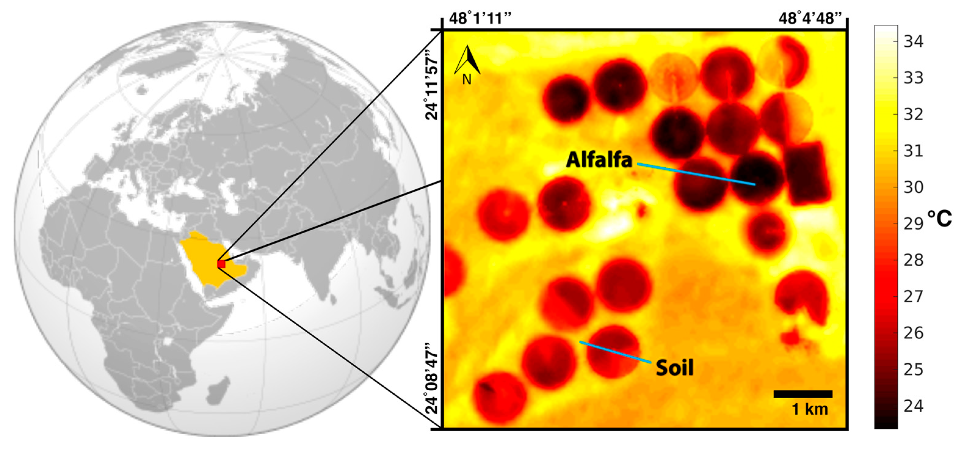
Figure 2.
(a) Landsat-based LST (in Celsius) calculated using the European Centre for Medium-Range Weather Forecasts (ECMWF) profile; (b) Normalized Difference Vegetation Index (NDVI) over the alfalfa field as derived from Landsat; and (c) in-situ LST (in Celsius) response for DOY 185, 256, and 336 at a single-point in the alfalfa field (see arrow in center panel) for the year 2015. The cross in (c) represents the Landsat overpass time (around 10:10 local time). Time is shown in Coordinated Universal Time (UTC).

Figure 3.
Comparison between: (a) in-situ and Landsat-based LST calculated from: (b) ECMWF; (c) National Centers for Environmental Prediction (NCEP); (d) Atmospheric Infrared Sounder (AIRS); (e) Moderate Resolution Imaging Spectroradiometer Atmospheric Profile Product from the Terra platform (MOD07); and (f) radiosonde (Integrated Global Radiosonde Archive, IGRA) atmospheric profiles over bare soil. The top panel (a) illustrates the in-situ based LST as derived from the Apogee radiometers and the aerosol optical depth (AOD) from the MODIS Gridded Atmospheric Product (MOD08), time coincident with the Landsat overpasses (i.e., approximately 10:10 a.m. local time). Panels b–f show ΔLST (Landsat minus in-situ LST) for the different atmospheric profile sources (in Celsius). The bottom x-axis (f) represents the DOYs for 2015. There were 24 scenes (instead of 28 for the rest) available for the radiosonde LST.

Figure 4.
Comparison between: (a) in-situ and Landsat-based LST calculated from: (b) ECMWF; (c) NCEP; (d) AIRS; (e) MOD07; and (f) radiosonde atmospheric profiles over alfalfa. Panels b–f show ΔLST (Landsat minus in-situ LST) for the different atmospheric profile sources (in Celsius). The bottom x-axis (f) represents the DOYs for 2015. Similar to Figure 3, the number of available scenes for the radiosonde LST is reduced by four. Large differences between satellite and in-situ LST are seen following a harvest (DOYs 185, 224, 256, and 288) as illustrated by the NDVI plot on the (a) top panel.
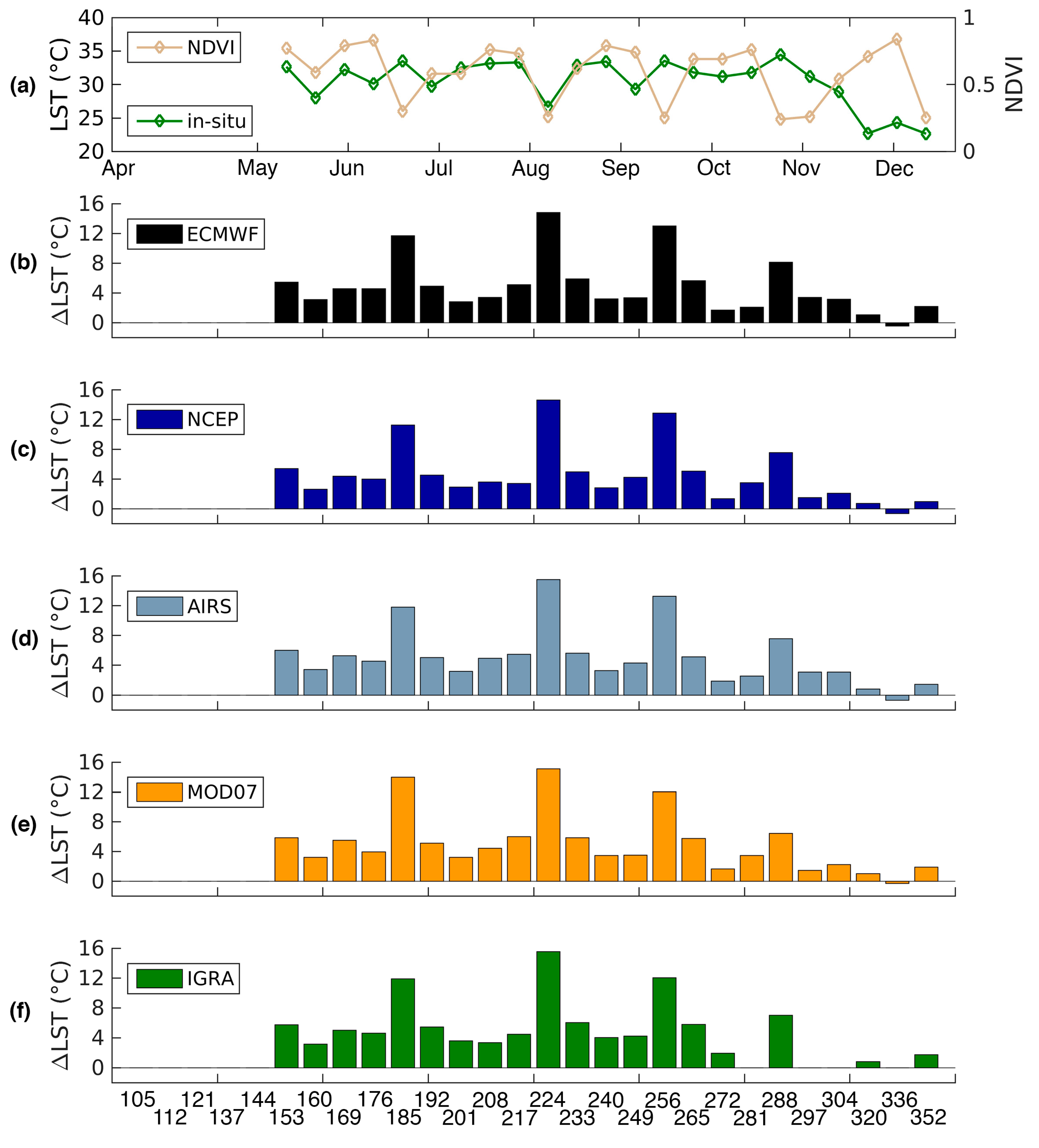
Figure 5.
Example of the relative humidity (RH, solid line) and temperature (T, dashed line) profile examples used in this analysis for: (a) DOY 105; (b) DOY 240; and (c) DOY 288 in 2015 from AIRS, ECMWF, NCEP, MOD07, and radiosonde. AIRS and ECMWF seem to be able to adequately represent the radiosonde measurements.
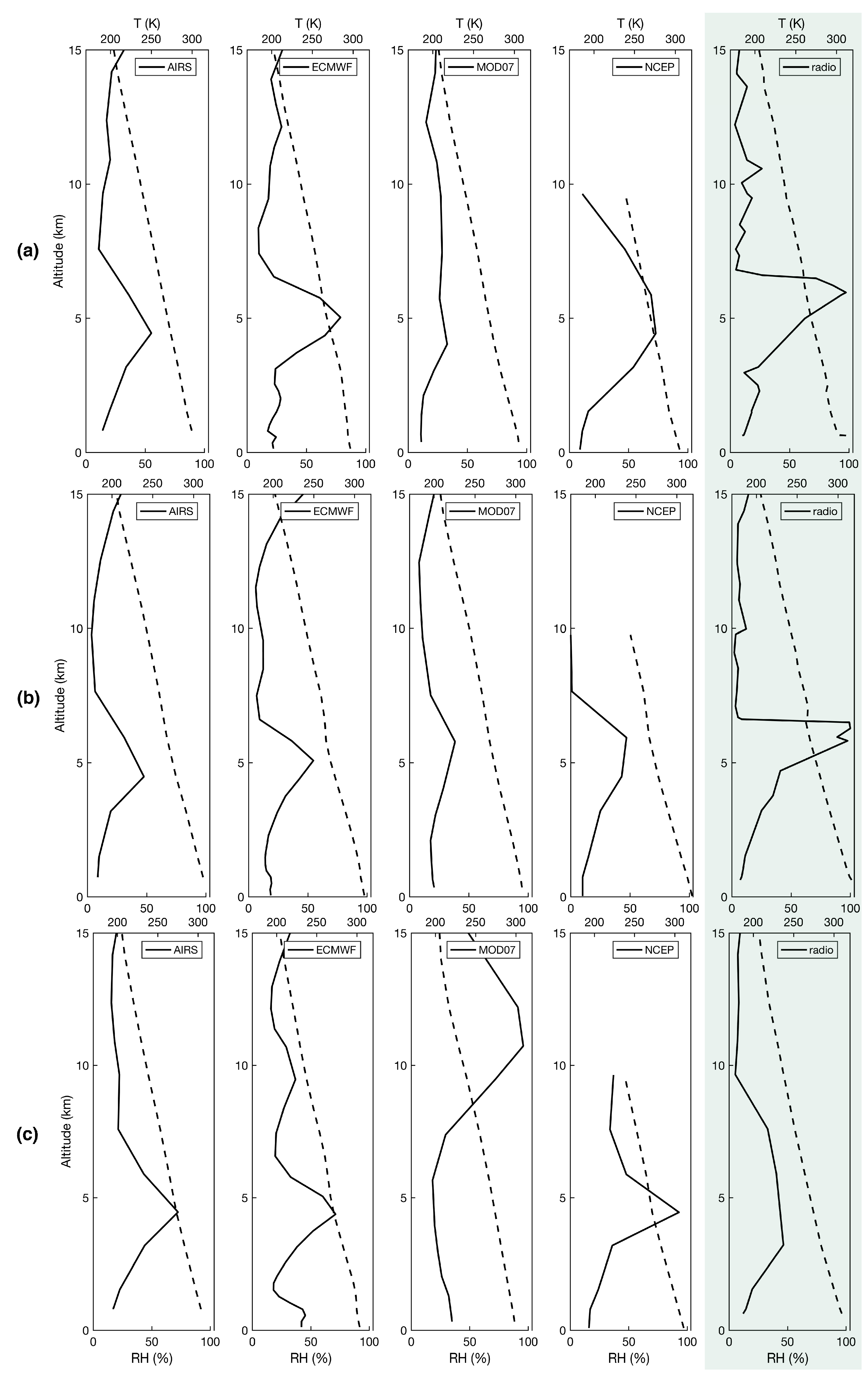
Figure 6.
Land surface temperature absolute differences over: bare soil (a–d); and alfalfa (e–h), when introducing randomly distributed errors of 15% to relative humidity (RH), 1 K to temperature (T), 40 ppmv to CO2, 30 Dobson units to O3, to AOD, and 0.01 to emissivity (e) to all the atmospheric profile sources. Errors in RH and ε produce the largest errors in LST for all the profile sources. Red crosses represent values outside of 1.5 standard deviations (black whiskers) from 25% and 75% of the distribution (blue box), while the red line represents the median.

Figure 7.
Land surface temperature absolute differences over bare soil when introducing randomly distributed errors of 5%, 10%, 15%, and 20% in RH, T, AOD and ε (e.g., for relative humidity: RH05, RH10, RH15, and RH20) to the: (a) ECMWF; (b) NCEP; (c) AIRS; and (d) MOD07 atmospheric profiles. Errors in RH and ε produce the largest errors in LST. Red crosses represent values outside of 1.5 standard deviations (black whiskers) from 25% and 75% of the distribution (blue box), while the red line represents the median.
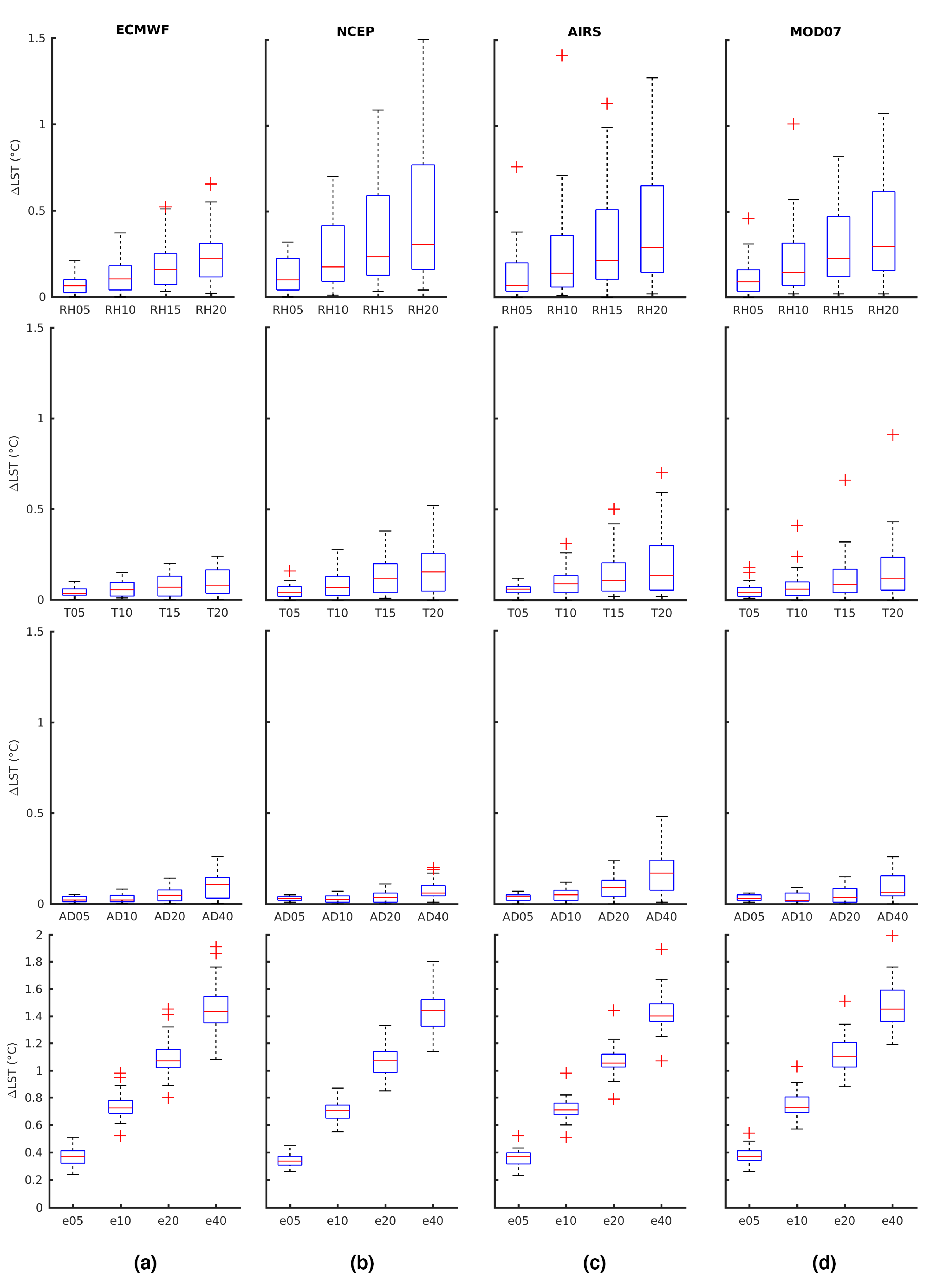
Figure 8.
Land surface temperature absolute differences over alfalfa when introducing randomly distributed errors of 5%, 10%, 15%, and 20% in RH, T, AOD and ε to the (a) ECMWF; (b) NCEP; (c) AIRS; and (d) MOD07 atmospheric profiles. Similar to Figure 7, errors in RH and ε produce the largest errors in LST. Red crosses represent values outside of 1.5 standard deviations (black whiskers) from 25% and 75% of the distribution (blue box), while the red line represents the median.
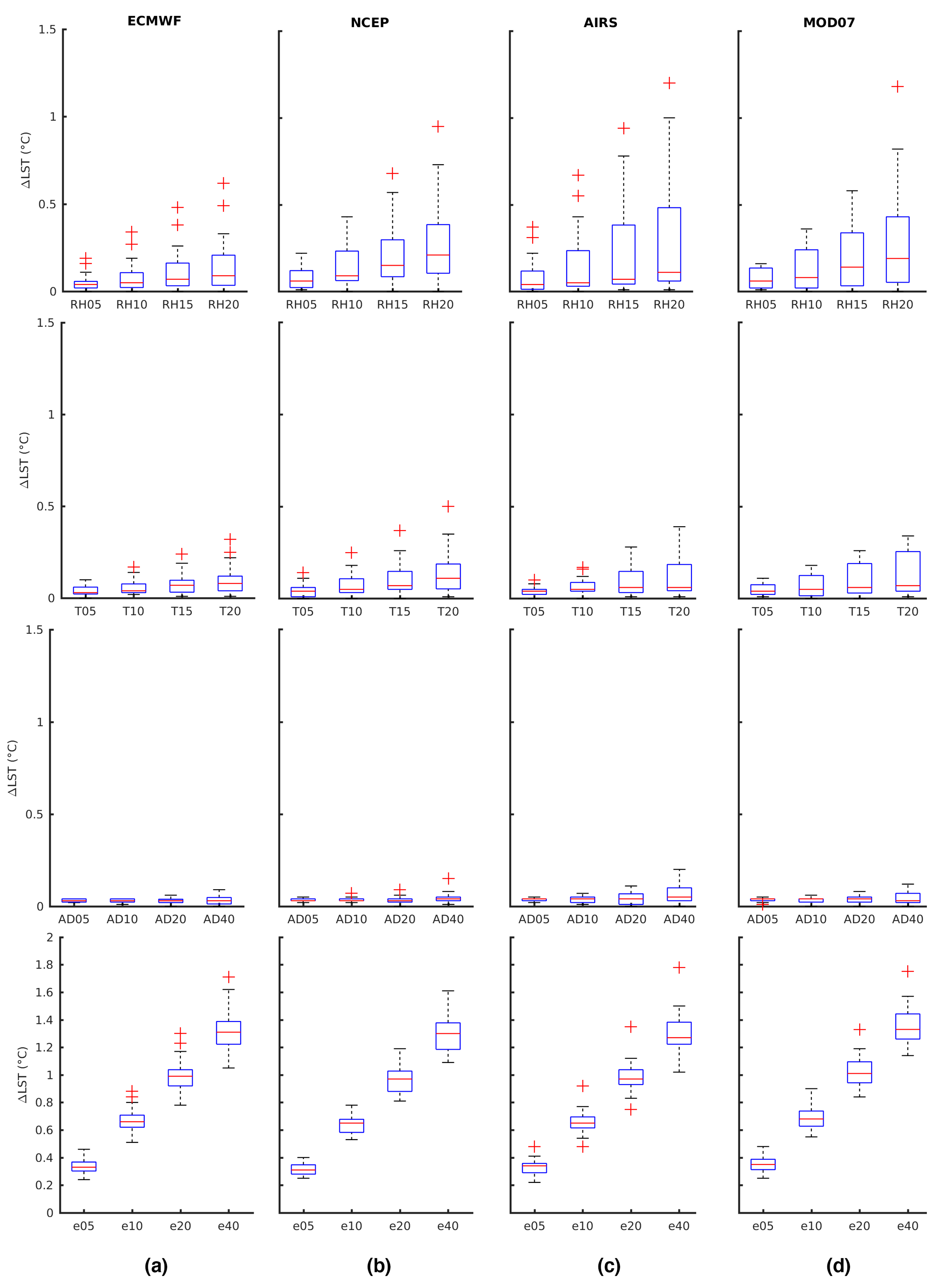

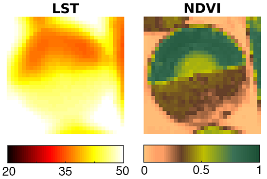
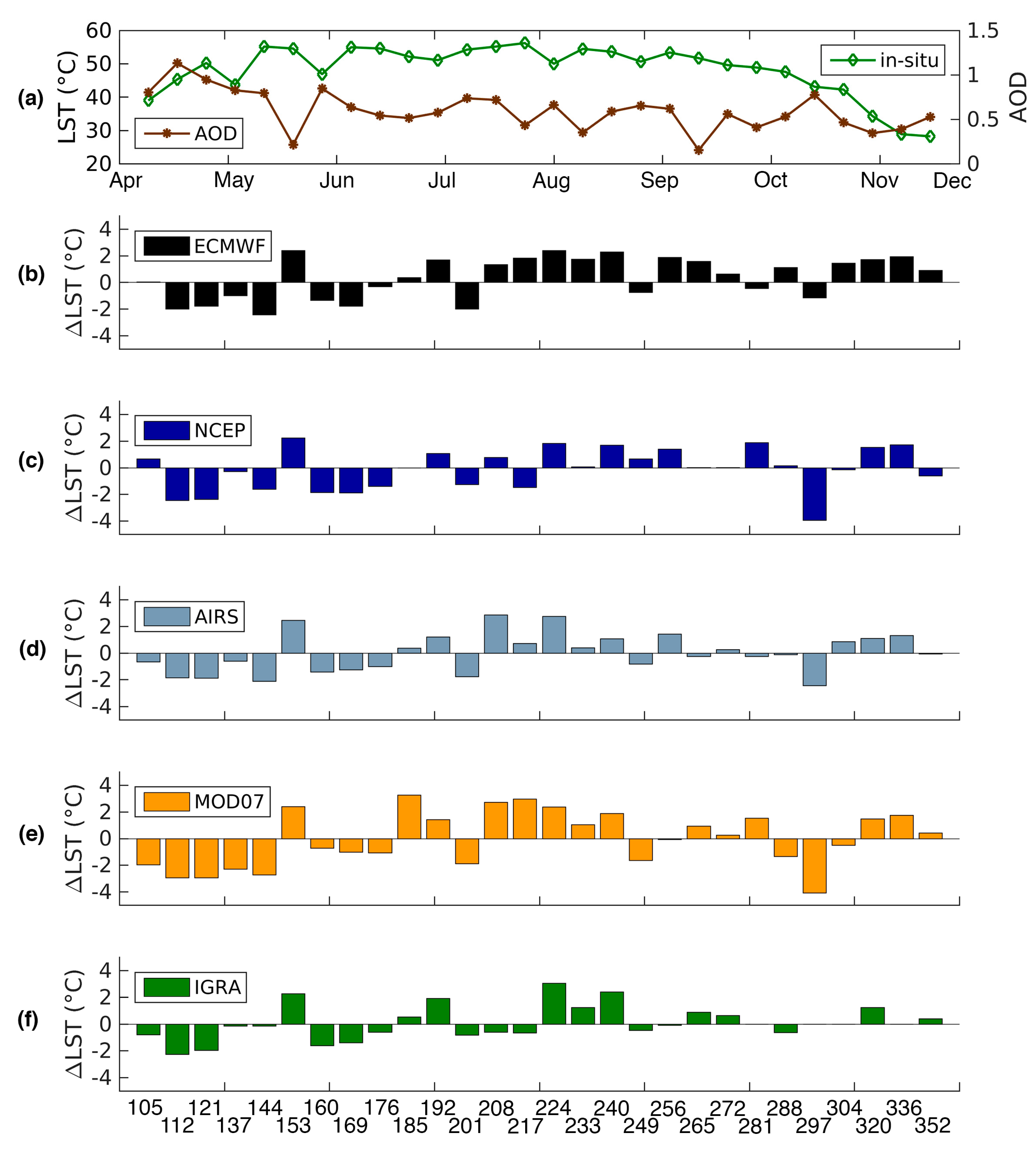
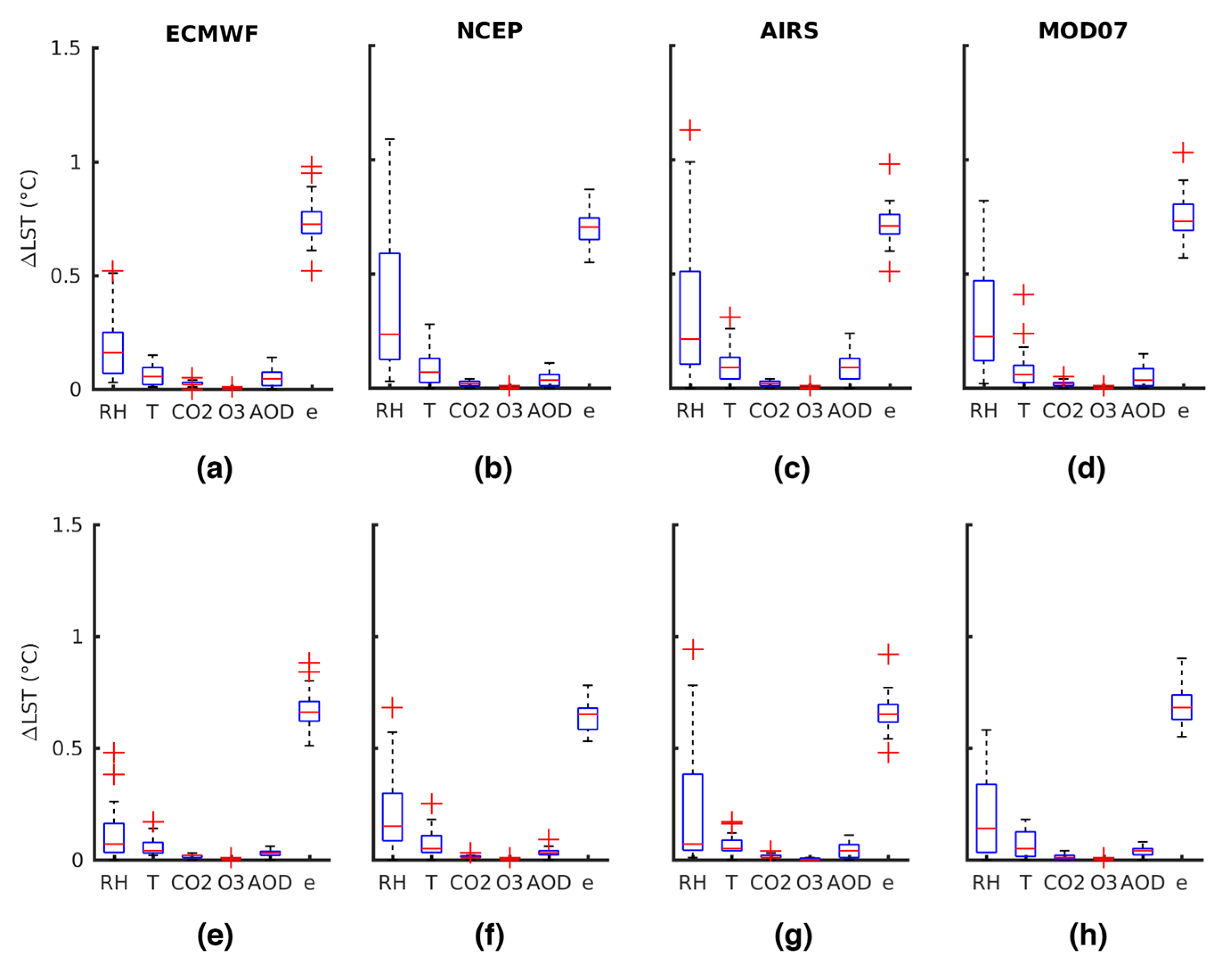
Table 1.
Statistical measures describing the agreement between satellite-derived and in-situ measured LST. Results are shown for soil, alfalfa, and alfalfa following a temporal-based NDVI filter. Alfalfa LST error is significantly reduced when incorporating the NDVI filter. Note that the radiosonde (IGRA*) statistics are not completely comparable with the other profile results, as they are based on a lower number of Landsat scenes (24).
| Atm. Profile | MAE | ME (Bias) | RMSE | |||||||||
|---|---|---|---|---|---|---|---|---|---|---|---|---|
| Soil | Alfalfa | Alfalfa (Filt.) | Soil | Alfalfa | Alfalfa (Filt.) | Soil | Alfalfa | Alfalfa (Filt.) | Soil | Alfalfa | Alfalfa (Filt.) | |
| ECMWF | 1.44 | 4.95 | 3.57 | 0.37 | 4.92 | 3.52 | 1.58 | 6.14 | 3.90 | 0.96 | 0.64 | 0.91 |
| NCEP | 1.25 | 4.57 | 3.31 | −1.13 | 4.52 | 3.24 | 1.56 | 5.86 | 3.60 | 0.96 | 0.64 | 0.93 |
| AIRS | 1.19 | 5.12 | 3.82 | 0.01 | 5.06 | 3.74 | 1.44 | 6.31 | 4.14 | 0.97 | 0.65 | 0.93 |
| MOD07 | 1.77 | 5.03 | 3.80 | −0.03 | 5.00 | 3.77 | 2.03 | 6.30 | 4.17 | 0.94 | 0.64 | 0.93 |
| IGRA* | 1.12 | 5.61 | 4.17 | 0.10 | 5.62 | 4.17 | 1.37 | 6.71 | 4.42 | 0.96 | 0.60 | 0.91 |
© 2017 by the authors. Licensee MDPI, Basel, Switzerland. This article is an open access article distributed under the terms and conditions of the Creative Commons Attribution (CC BY) license (http://creativecommons.org/licenses/by/4.0/).
Share and Cite
MDPI and ACS Style
Rosas, J.; Houborg, R.; McCabe, M.F. Sensitivity of Landsat 8 Surface Temperature Estimates to Atmospheric Profile Data: A Study Using MODTRAN in Dryland Irrigated Systems. Remote Sens. 2017, 9, 988. https://doi.org/10.3390/rs9100988
AMA Style
Rosas J, Houborg R, McCabe MF. Sensitivity of Landsat 8 Surface Temperature Estimates to Atmospheric Profile Data: A Study Using MODTRAN in Dryland Irrigated Systems. Remote Sensing. 2017; 9(10):988. https://doi.org/10.3390/rs9100988
Chicago/Turabian StyleRosas, Jorge, Rasmus Houborg, and Matthew F. McCabe. 2017. "Sensitivity of Landsat 8 Surface Temperature Estimates to Atmospheric Profile Data: A Study Using MODTRAN in Dryland Irrigated Systems" Remote Sensing 9, no. 10: 988. https://doi.org/10.3390/rs9100988
Note that from the first issue of 2016, this journal uses article numbers instead of page numbers. See further details here.