A Rigorously-Weighted Spatiotemporal Fusion Model with Uncertainty Analysis


Institute of Space and Earth Information Science, Chinese University of Hong Kong, Shatin, Hong Kong, China
*
Author to whom correspondence should be addressed.
Remote Sens. 2017, 9(10), 990; https://doi.org/10.3390/rs9100990
Submission received: 14 August 2017
/
Revised: 18 September 2017
/
Accepted: 21 September 2017
/
Published: 25 September 2017
(This article belongs to the Special Issue Remote Sensing Image Downscaling)
Abstract
:Interest has been growing with regard to the use of remote sensing data characterized by a fine spatial resolution and frequent coverage for the monitoring of land surface dynamics. However, current satellite sensors are fundamentally limited by a trade-off between their spatial and temporal resolutions. Spatiotemporal fusion thus provides a feasible solution to overcome this limitation, and many blending algorithms have been developed. Among them, the popular spatial and temporal adaptive reflectance fusion model (STARFM) is based on a weighted function; however, it uses an ad hoc approach to estimate the weights of surrounding similar pixels. Additionally, an uncertainty analysis of the predicted result is not provided in the STARFM or any other fusion algorithm. This paper proposes a rigorously-weighted spatiotemporal fusion model (RWSTFM) based on geostatistics to blend the surface reflectances of Moderate Resolution Imaging Spectroradiometer (MODIS) and Landsat-5 Thematic Mapper (TM) imagery. The RWSTFM, which is based on ordinary kriging, derives the weights in terms of a fitted semivariance-distance relationship and calculates the estimation variance, which is a measure of the prediction uncertainty. The RWSTFM was tested using three datasets and compared with two commonly-used spatiotemporal reflectance fusion algorithms: the STARFM and the flexible spatiotemporal data fusion (FSDAF) method. The fusion results show that the proposed RWSTFM consistently outperformed the other algorithms both visually and quantitatively. Additionally, more than 70% of the squared error was accounted for by the estimation variance of the RWSTFM for all three of the datasets.
1. Introduction
Dense time-series satellite images with fine spatial resolutions constitute broad applications in the monitoring of vegetation dynamics, forest biophysical properties and land cover changes. However, due to technical limitations, there is a trade-off between the spatial and temporal resolution of currently-utilized satellite sensors. No single sensor can simultaneously achieve both a fine spatial resolution and a frequent revisit cycle, although a large number of remote sensing instruments with different spatial, temporal and spectral characteristics have been launched. For example, Landsat sensors have fine spatial resolutions (30 m), but long revisit frequencies (16 days) [1,2]. In contrast, the Moderate Resolution Imaging Spectroradiometer (MODIS) instrument has a high temporal resolution of one day, but a coarse spatial resolution of 250–1000 m [3,4]. Thus, the combination of complementary remote sensing datasets could provide a feasible solution to circumvent the limitations of current satellite sensors.
Existing spatiotemporal fusion methods have integrated the advantages of both Landsat and MODIS data to generate fused satellite images with fine spatial and temporal resolutions for expanded applications [5,6,7,8]. These methods can be categorized as weighted function methods, unmixing methods and dictionary-pair learning methods. Other relatively uncommon methods are also used and are based on Bayesian [9,10], neural network [11,12], pyramid [13] and semi-physical model [14] methods. Among the weighted function-based methods, the spatial and temporal adaptive reflectance fusion model (STARFM) method [15] was developed in 2006 to predict the daily Landsat surface reflectance by blending MODIS and Landsat surface reflectance data. This method calculates the surface reflectance through spectrally similar neighboring pixels weighted by spectral, temporal and spatial distances within a moving window. This method has since been improved by the spatial temporal adaptive algorithm for mapping reflectance change (STAARCH) [16] and the enhanced STARFM (ESTARFM) method [17] to overcome existing landscape disturbance limitations and heterogeneous landscape problems, respectively.
Zhukov et al. [18] developed an unmixing method for image fusion to predict imagery with fine spatial and spectral resolutions, which has been greatly applied in spatiotemporal fusion [19,20,21,22]. Based on such an unmixing method, Amoros-Lopez et al. [23] subsequently alleviated unrealistic estimated spectra and decreased unmixing errors by regularizing the cost function. Huang and Zhang [24] proposed a constrained linear unmixing method for both phenological and land cover changes. Wu et al. [25,26] calculated the reflectance change by the weighted linear mixed method and added the estimated change to the fine-resolution image on the base date to generate the fusion result. Zhu el al. [27] proposed a flexible spatiotemporal data fusion (FSDAF) method based on the unmixing method and thin plate spline interpolator. In particular, this method could closely capture reflectance changes caused by land cover conversion, which is a big challenge for current spatiotemporal data fusion methods.
A dictionary pair learning-based super-resolution method known as the sparse representation-based spatiotemporal reflectance fusion model (SPSTFM) was proposed by Huang and Song [28] to predict phenological changes and land cover changes uniformly. The SPSTFM is employed to train dictionaries generated from difference image patches (i.e., between fine and coarse resolutions), to establish a correspondence between structures of fine- and coarse-resolution images through sparse representation and to reconstruct fine-resolution images for the prediction date via sparse coding. Song and Huang [29] presented a continual two-stage framework based on one-pair image learning that is described as follows: first, the spatial resolution of MODIS data on a base and a prediction date is improved simultaneously by means of sparse representation; second, known Landsat and super-resolved MODIS images are fused via high-pass modulation to generate Landsat data for the prediction date. Subsequently, Wu et al. [30] developed an error-bound-regularized sparse coding for spatiotemporal reflectance fusion model (EBSPTM) to model the possible perturbations of an overcomplete dictionary and formulate dictionary perturbations to represent a sparse elastic net regression problem.
Each of the abovementioned methods can improve the spatial and temporal resolutions of satellite images for specific applications. However, both weighted function-based methods and other spatiotemporal methods apply an ad hoc approach to calculate the weights of neighboring similar pixels during the fusion process. In addition, they are unable to provide an uncertainty analysis of the prediction results. It is impossible to exactly describe the predicted outcome using the above methods, but the outcome could be estimated using geostatistical methods. Meanwhile, the surface reflectance observed within a remote sensing image is spatially dependent, i.e., pixel locations immediately adjacent to one another are more similar than pixel locations across larger distances. Geostatistics is typically applied to analyze regionalized observations of variables that are distributed throughout space. The geostatistical approach known as kriging [31] has gained special acceptance as a tool for the interpolation of many types of data, including the surface temperature, precipitation, soil properties and elevation [32,33,34]. Kriging has been utilized for the downscaling of Landsat and MODIS images [35,36,37] and pansharpening during Sentinel-2 fusion tasks [38]. Kriging was developed to achieve the best linear unbiased prediction (BLUP) and obtain the optimum weights in terms of the fitted semivariance-distance relationship. Kriging can also be used to compute the minimized estimation variance, otherwise known as the kriging variance, which can be used as a measure of the prediction uncertainty [39,40]. On the basis of the above considerations, this paper proposes a rigorously-weighted spatiotemporal fusion model (RWSTFM) based on the geostatistical ordinary kriging method. The RWSTFM possesses the following strengths. First, it utilizes the abovementioned advantages of kriging methods to simultaneously obtain the rigorously weighted function of a spatiotemporal fusion method and the estimation variance of kriging output as a quality indicator of the estimator. Second, it describes land cover changes and unchanged areas separately. For unchanged land cover areas, the method searches for similar pixels around the location of the central pixel in a fine-resolution image, while for changed land cover areas, it searches for spectrally similar pixels in a coarse-resolution image acquired on the base date , which has similar spectral characteristics to a given pixel in a coarse-resolution image acquired on the prediction date . The process of searching for spectrally similar pixels considers the structural similarity throughout the changed land cover areas. The searched spectrally similar pixels in the coarse- and fine-resolution images can be applied to adjust the fusion value and predict changed areas more accurately. Hence, the RWSTFM integrates both changed and unchanged land cover areas in a uniform manner. We tested this method on three datasets from New South Wales, Australia, and compared the fusion results with those of the STARFM and FSDAF methods.
The rest of this paper is organized as follows. We introduce the theoretical basis and implementation steps of the RWSTFM in Section 2, while the test dataset and study area are described in Section 3. Section 4 provides the details of the experiments, and the strengths and limitations of the RWSTFM are discussed in the last section.
2. Methods
Differences in atmospheric conditions (e.g., clouds, fogs and aerosols), solar angle and altitude at different pixel locations and data pre-processing such as radiometric calibration, atmospheric correction and geometric rectification cannot completely remove this variability [17,41]. Furthermore, changes in the surface reflectance may differ among each pixel during an observation period. Thus, it is advisable to apply a local method that will act on each pixel and its neighboring pixels within a moving window. In the following subsections, we first display the theoretical basis of the RWSTFM and illustrate how the ordinary kriging method can be integrated into the spatiotemporal image fusion process. Then, we briefly introduce the ordinary kriging method. Third, we present the procedure of the RWSTFM for predicting the Landsat-like image and calculating the estimation variance. Finally, we provide several indices for an evaluation of the fusion results. We discuss the changed and unchanged land use areas with regard to their complex temporal dynamics in each corresponding band as follows. We suppose that the coarse-resolution sensor has similar spectral bands as the fine-resolution sensor.
2.1. Theoretical Basis
First, we assume that the land cover does not change from the date to the date .
For a given pixel , the difference in the reflectance between a coarse-resolution pixel and a fine-resolution pixel is affected by system errors among the different sensors. Therefore, the relationship between the coarse- and fine-resolution reflectance can be built as a linear model:
where and denote the surface reflectance for Landsat and MODIS data, respectively, is a given pixel location for either the Landsat or the MODIS image, is the acquisition date for both the MODIS and Landsat data and and are the coefficients of the linear regression model. Similarly, we have the following for another coarse-resolution image acquired on the date :
Suppose the system errors and the land cover type within the pixel do not change from date to . This model will have the same parameters, namely, , on the different observation dates. Consequently, we can obtain the predicted reflectance from Equations (1) and (2):
The fine-resolution reflectance at equals the sum of the fine-resolution reflectance at and the scaled change in the reflectance from to within the coarse-resolution images. can be derived by linearly regressing the reflectance values of spectrally similar neighboring pixels in the fine-resolution image and the corresponding coarse-resolution image on the base date . A search for spectrally similar pixels can be conducted within a moving window around the central pixel in the fine-resolution image at .
Next, we assume that the land cover changes from date to .
The assumption wherein the linear parameters and are equivalent for an unchanged land cover type is no longer reasonable, namely, . We introduce an adjustment factor l and make . Then, we can obtain the reflectance of a fine-resolution pixel at :
Subsequently, we can derive the predicted reflectance from Equations (1) and (4):
where . We assume that spectrally similar pixels in the MODIS data at have similar spectral characteristics (i.e., the same land cover type) as the corresponding pixels in the MODIS data at . Therefore, we search the entire MODIS image for the date and compare the neighbors of every pixel in the MODIS image at (as candidate pixels) with those of a given pixel (namely, the target pixel) in the MODIS image for the date We measure the similarity of the candidate and target pixels by calculating the spectral difference of neighboring pixel values in each band based on the sum of the Euclidean distance. The candidate pixel with the smallest spectral difference of neighbors is selected as the most similar pixel. This pixel is known as a spectrally-corresponding pixel to distinguish it from a spatially-corresponding pixel (with the same row and column). Then, can be obtained from the linear regression of the fine-resolution reflectance against the coarse-resolution reflectance for spectrally-corresponding pixels at . Similarly, is obtained from the linear regression of the fine-resolution reflectance against the coarse-resolution reflectance for spatially-corresponding pixels at according to Equation (3). Hence, the fine-resolution reflectance at equals the sum of the fine-resolution reflectance at with the scaled change of the modified reflectance at and the original reflectance at in the coarse-resolution images. When the land cover type does not change, . Note that Equation (3) is a special case of Equation (5). Thus, we can show that Equations (3) and (5) exhibit the same form.
The moving window is utilized to search for similar pixels within the local window to introduce additional information from neighboring pixels [15], and the information from these similar pixels is then integrated into the fine-resolution reflectance calculation. From all of the above, the fine-resolution surface reflectance of the central pixel on the date with a weighted function can be computed as a unified function regardless of the distribution of changed and unchanged areas:
where is the search window size, is the central pixel of the moving window, n is the number of similar pixels, is the location of a similar pixel with a central pixel, is the weight of the similar pixel and is the adjustment factor. Only the spectrally similar pixels retrieved from the Landsat surface reflectance values within the moving window are used for weights while predicting the reflectance. Weights of similar pixels can be derived using a geostatistical method such as ordinary kriging (Section 2.2). The search window size is determined by visual analysis of the homogeneity of the surface and considering the spatial resolution ratio of coarse to fine resolution images. For example, the search window size is set to about 15–17 as the spatial resolution ratio of MODIS to Landsat images is almost 16 (calculated by 500/30). If the regional landscape is more homogeneous, the value of can be smaller. Otherwise, it will be set larger. The selection of the parameter will be validated by the performance of experiments. Equation (6) indicates that the fine-resolution reflectance on the prediction date equals the weighted average of the fine-resolution reflectance values observed on the base date added to the change in the modified coarse-resolution reflectance.
2.2. Weighting via Ordinary Kriging
Kriging [42] is a geostatistical technique that is employed to obtain the BLUP by assigning an optimum set of weights to all of the available and relevant observation data.
Suppose that the dataset can be denoted using observations from a geographic space, where is a location, and are the coordinates and is the number of observations. represents the unknown observation of . We assume that the dataset Z has spatially homogenous properties for purely coarse-resolution pixels or end-members belonging to the same land cover type for mixed coarse-resolution pixels. The stationarity and isotropy of radiometric behavior are reasonable assumptions when we apply geostatistics to conduct remote sensing surface reflectance analysis within a local area [31,43]. Hence, we can obtain observations from the dataset that have the same expected values and variance:
The kriging predictor is a weighted average of neighboring observations:
where is the predictor of , are the weights associated with the sampling points and is the zero-mean regression residual. The BLUP is obtained by minimizing the kriging variance:
According to the above assumption of Equation (7), we can get the following:
Hence, we can infer that Equation (9) is subject to:
With the minimizing target function of Equation (9) and the linear constrained condition (11), Lagrange’s method of multipliers can be used to solve this conditional extremum problem. Set F as the Lagrange function:
where is a Langrange multiplier, and the function can be derived by and . Thus, we can derive the optimal values from the matrix equation:
where:
Here, we introduce the semivariance:
The semivariance and distance can be derived from known sample points, and they can be fitted using a variogram function and an extra nugget model that captures the nugget effect. is a matrix of semivariances between all of the data points and is constructed using the variogram function. is a vector of the estimated semivariances between the data points and the point at which we wish to predict the unknown variable , and represents the resulting weights and .
Thus, the optimal linear predictor is as follows:
Furthermore, the kriging variance is
In practice, we select spectrally similar pixels from a local neighborhood around the prediction location, i.e., the kriging search neighborhood [44]. The search neighborhood of a given pixel includes enough pixels to infer the statistics (e.g., semi-variograms) for each local area. After this step, we can calculate the weights () from similar pixels within the moving window in the Landsat image acquired on the base date () using the kriging method. Thus, the derived weights () (identical to the weights ()) can be used to predict the fine-resolution image for the prediction date () as described in Equation (6).
2.3. Process of the RWSTFM Implementation
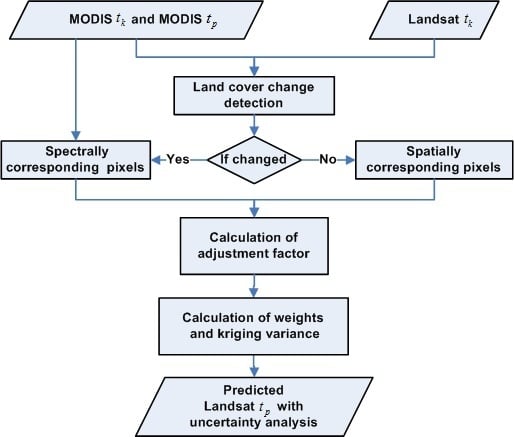
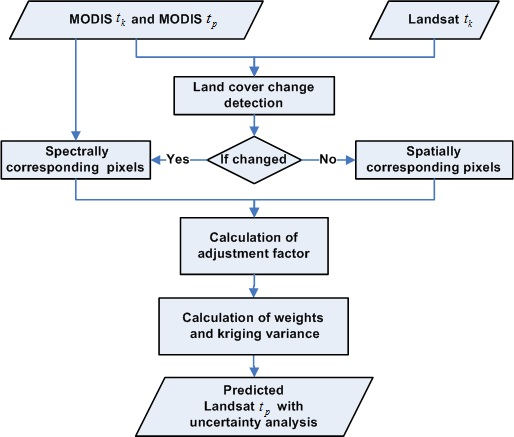
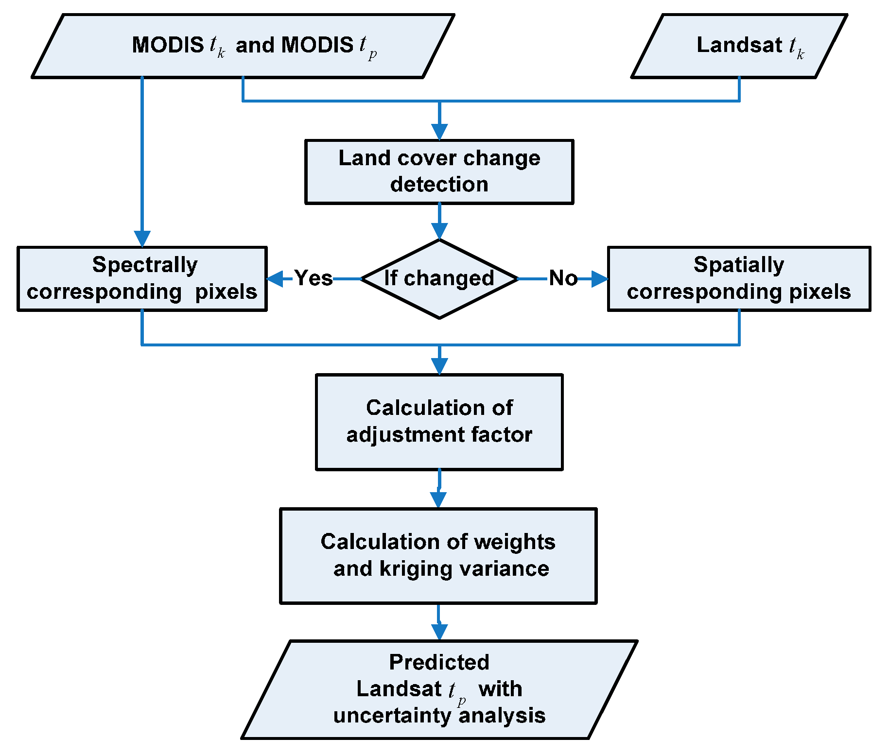
Figure 1 presents the flowchart of the RWSTFM. There are four steps in the implementation of the RWSTFM: detecting land cover changes, calculating the adjustment factors and searching for similar pixels, calculating the weights for similar pixels and the kriging variance and predicting the fine-resolution image with uncertainty analysis. All of these steps are discussed in detail hereafter.
First, we adopt a thresholding method to detect the changes in the surface reflectance images at different dates:
where are the average values of the three bands (such as near infrared, or NIR, red and green bands of the Landsat and MODIS images) at the location at and for the Landsat and MODIS data, respectively, and and are the absolute difference maps. The corresponding thresholds are set as and , which denote the average values of absolute difference maps. If both of the absolute values of a given pixel lie beyond the designated thresholds (), the land cover will be marked as changed. For all other cases, this means that the land cover is nearly the same as that on the base date and is essentially unchanged.
Second, we calculate the adjustment factor for both changed and unchanged land cover areas. For changed land cover areas, . We apply a linear regression to the Landsat image against the corresponding MODIS image at within the spectrally similar pixels to obtain . We search the entire MODIS image at and find the spectrally-corresponding pixel for the regression of . In addition, we consider the structural similarity between spectrally-corresponding pixels in the MODIS image at and the target pixel in the MODIS image at by extracting edge information. We detect the edges using a Gaussian high-pass filter. Subsequently, we search for similar pixels along the same edge areas when the MODIS pixel at is detected as an edge pixel. Conversely, we search for similar pixels within the non-edge areas when the MODIS pixel at is not detected as an edge pixel. Furthermore, we apply linear regression to the Landsat image against the spatially corresponding MODIS image with similar pixels within a local window at to obtain . Finally, we obtain the adjustment factor via the ratio of to . Since the regression is conducted on neighboring similar pixels, a fine-resolution image acquired on the base date is used to search for pixels similar to the central pixel within a local window. For unchanged land cover areas, . Thus, for unchanged pixels, the calculation of the parameter is a special circumstance involving changed pixels. Following this step, we can obtain the parameter of for both changed and unchanged areas.
Third, we calculate the weights and the kriging variance using an ordinary kriging method. We apply a variogram function to fit the relationship between the distance and semivariance in the spectrally similar neighbor pixels of a given pixel in the Landsat image at . Subsequently, we calculate the weights of spectrally similar neighbor pixels and the kriging variance using an ordinary kriging algorithm (Section 2.2).
Finally, we predict the fine-resolution reflectance and calculate the estimation variance on the prediction date. After we obtain these two parameters, we can predict the fine-resolution reflectance at for both changed and unchanged land cover areas according to Equation (6). Meanwhile, we can calculate the estimation variance (). The kriging estimation variance is the non-conditional minimized estimation variance and represents a measure of the accuracy of the local estimation from similar pixels. However, the kriging method acts on similar pixels within a local window in the fine-resolution image at , and the kriging variance () denotes the prediction variance of the fine-resolution image at rather than at . Thus, the prediction variance must be corrected by adding the squared deviations between the coarse-resolution images on the prediction date and the base date to the kriging variance:
where is the estimation variance of the fine-resolution image at , is the kriging variance, and and are the actual MODIS reflectance values for a given pixel at and , respectively.
2.4. Evaluation Indices
We evaluated the fusion results using quality indices, namely the root mean square error (RMSE), correlation coefficient (CC), average absolute difference (AAD), average difference (AD) and structure similarity (SSIM) for every band. The RMSE is used to assess the differences between the predicted and reference images. Smaller values indicate a closer match. The CC reflects the degree of correlation (i.e., similarity) between the predicted and reference images. A value that is closer to one indicates a strong linear relationship between the images. The AAD and AD are used to measure the average bias for an individual prediction. The SSIM is used to assess the similarity of the structures between the predicted and reference images. An SSIM value closer to 1 indicates more structural similarity. The erreur relative globale adimensionnelle de synthese (ERGAS) [45] is used to evaluate the fusion results of all three bands (i.e., the NIR, red and green bands). If the ERGAS value is greater than 3, the fusion product is regarded as low quality. If the ERGAS value is lower than 3 or close to zero, the fusion product is satisfactory.
3. Study Area and Datasets
For the experiments, we organized three datasets that are located in northern New South Wales, Australia (149.2815°E, 29.0855°S). New South Wales is a rice-based irrigation region along the eastern coast of Australia. Its borders comprise Queensland to the north, Victoria to the south and South Australia to the west. Rice, soybeans, corn and sorghum constitute the summer crops, which are primarily irrigated from October–November, grown from December–April and harvested by May. In addition, cereals and pastureland grow during the winter (i.e., June–August).
The Landsat-5 TM and MODIS images were provided by Emelyanova et al. [46] and have been atmospherically corrected, calibrated and co-registered. These images cover three different study sites with contrasting spatial and temporal dynamics. The first image constitutes primarily phenological changes; the second exhibits primarily land cover changes; and the third reveals both phenological and land cover changes.
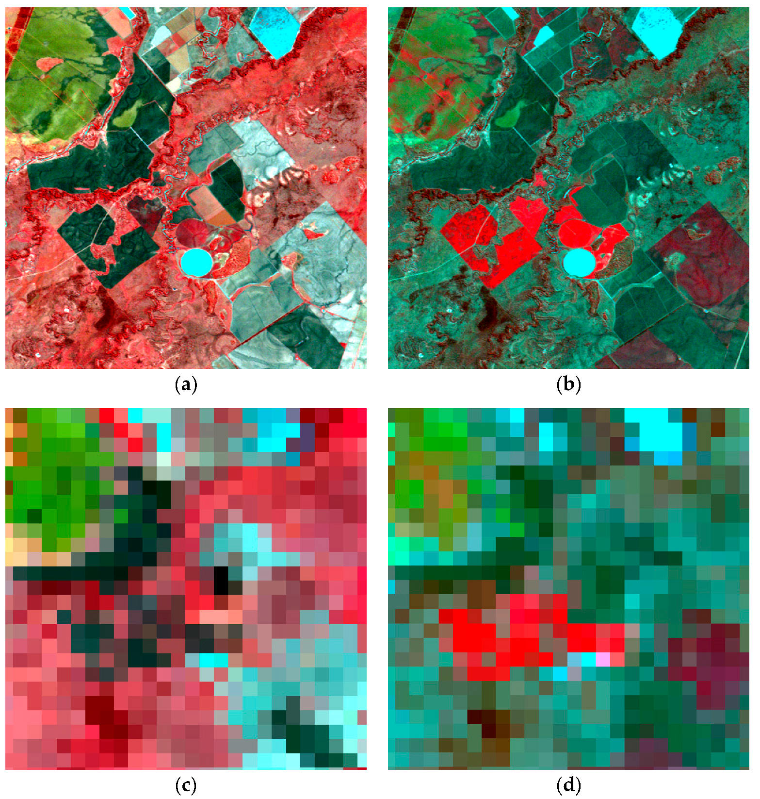
The first dataset that constitutes primarily phenological changes has 480 × 480 pixels with three bands. Figure 2 displays false color composites using Bands 4 (NIR), 3 (red) and 2 (green) of the Landsat image and the corresponding Bands 2, 1 and 4 of the MODIS image as a red-green-blue composite. The two Landsat images were acquired on 2 May 2004 and 5 July 2004. Fewer shape, texture and size changes are observed, but many phenological changes can be detected. For example, a large part of the summer cropland (i.e., rice) is harvested in July, while some vegetation (i.e., cereals) is growing during the winter.
The images for the second data site that primarily reveal land cover changes were acquired on 26 November 2004 and 28 December 2004. As a large flood occurred in December 2004, a large proportion of the land cover types abruptly changed to water in some of the pixels (i.e., the black pixels in Figure 3b). The crops are in their growing season from November–December. The crop pixels in December are slightly darker than in November. However, the phenological changes are not as evident and are relatively subtle. The image size is 480 × 480 × 3 pixels.
The images for the third data site exhibiting both phenological and land cover changes were acquired on 25 October 2004 and 12 December 2004. Since a large flood occurred in December 2004 and because the crops were irrigated in October and grown in December, this data site illustrates both phenological changes and land cover changes. A large field of crops is inundated as represented by the blue and black areas (Figure 4b). Other fields also exhibit gradual changes (phenological changes). The image size is 800 × 800 × 3 pixels.
4. Experiments and Discussion
We used the three datasets for New South Wales to test the performance of the RWSTFM and to subsequently compare our results with those of two well-known methods: the STARFM and FSDAF. Both of these established methods only require one pair of fine- and coarse-resolution images to predict fusion results.
4.1. Test Using the First Dataset to Detect Phenological Changes
Figure 5 shows the actual Landsat image on 5 July 2004 and the fusion results predicted using the three methods. We applied the STARFM method with a max search distance of 630 m and the FSDAF method with a half-window size of 40 pixels to acquire reflectance information for neighboring pixels. From a visual comparison, the images predicted using the three methods are generally similar to the original Landsat image (Figure 5a). Hence, all of the methods are able to capture the general phenological changes in the croplands during this observation period. However, the STARFM image presents some color mixing in the changed areas and fails to maintain the clear edges of parcels in the croplands. The FSDAF method preserves the shapes of the parcels in the larger areas with phenological changes. However, the FSDAF method smooths some of the inner details and generates some confusion in the adjacent boundaries; these results may be caused by the classification method, which cannot classify very similar categories, may omit select smaller categories and could lead to a collinearity problem during the solutions of the equations in the unmixing method. Hence, reassigning the values of the fine-resolution pixels for the same end-member will lead to some errors and missing spatial details. Although the FSDAF method adopts a thin plate spline method to guide the residual distribution, which improves the accuracy greatly, the method is still insufficient for retrieving all of the spatial details. The results of the RWSTFM seem to be more similar to the actual image and retain more spatial details than the STARFM and FSDAF methods. We also evaluate the fusion results using several objective indices (Table 1). Compared with the results obtained using the STARFM and FSDAF methods, the RWSTFM results have smaller RMSE and AAD values, higher CC and SSIM values in every band and a smaller ERGAS value overall. With regard to the overall prediction bias, STARFM and FSDAF methods have higher biases () than the RWSTFM method. Among these three methods, the RWSTFM results demonstrate the smallest errors and the highest similarity to the actual image. The FSDAF method has higher CC and SSIM values for Bands 3 and 4 than the STARFM method, while it has smaller CC, SSIM and higher RMSE values for Band 2. Furthermore, the FSDAF method has higher AAD and AD values for every band and a higher ERGAS value overall than the STARFM method.
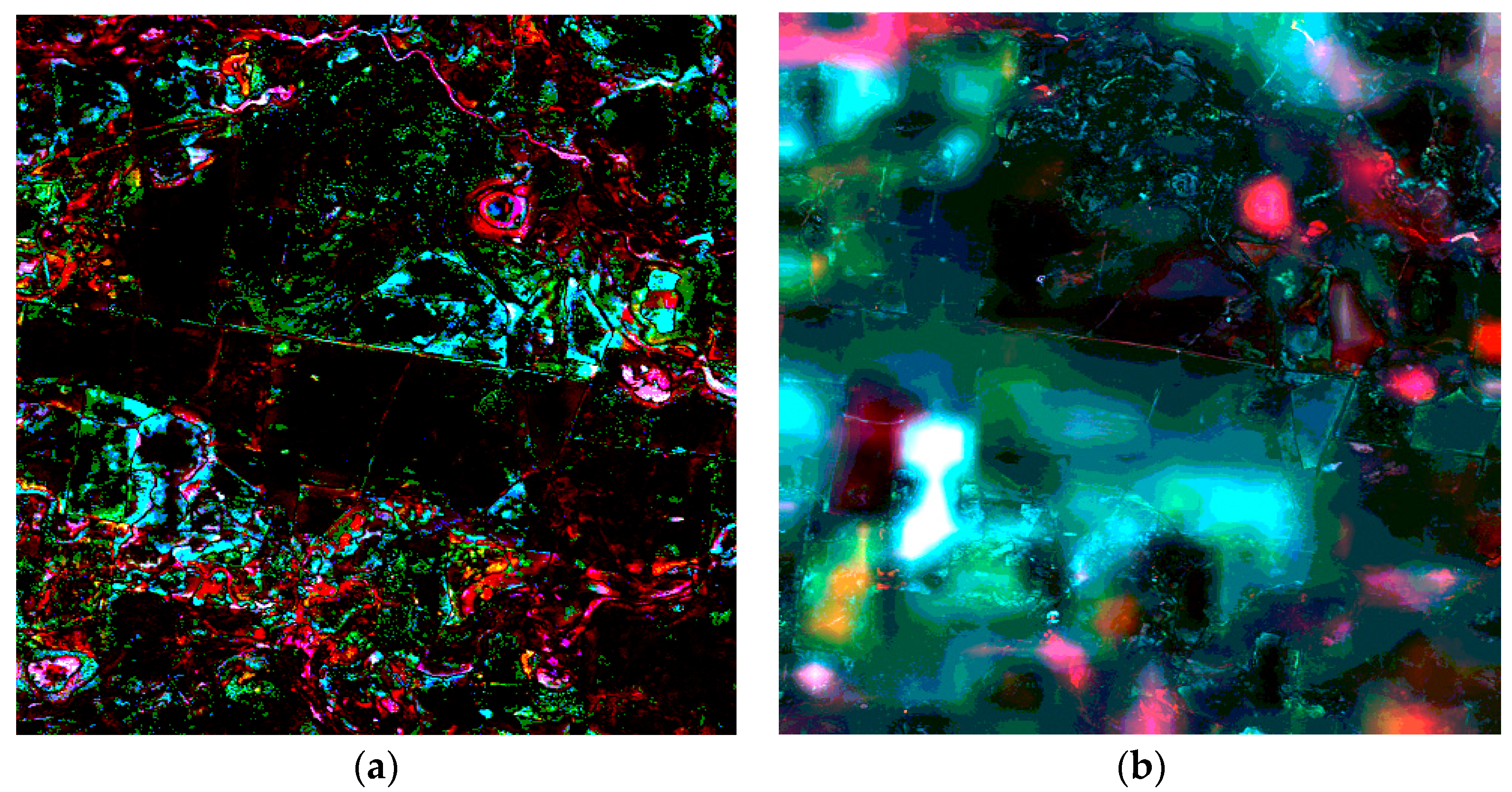
Figure 6a shows the squared error map derived by comparing the fusion image predicted using the RWSTFM with the actual Landsat image on 5 July 2004. Figure 6b shows the estimation variance map calculated from each pixel using the RWSTFM. Some overlapping areas can be observed between the squared error and estimation variance results. The changed areas and the edges of some objects show high values in the squared error map. We can also see that the estimation variance is unevenly distributed. Homogeneous areas and unchanged land cover areas, including some larger parcels of the cropland, have lower estimation variances. In contrast, the shapes and edges of surface objects and changed areas have higher estimation variances. Because each area has a different spectrum, each band reveals a large difference in the uncertainty map.
To assess how well the prediction uncertainty reflects the prediction error, we calculate the percentage of the squared error () that is lower than the estimation variance () in each band (Table 2). A percentage that is higher than 68.26% indicates that more than 68.26% of the prediction error is covered by the estimation uncertainty. Additionally, according to the three-sigma limits (P() = 68.26%) of a normal distribution, the prediction error falls within the confidence interval (i.e., the amount of uncertainty) at an almost 70% confidence level. Table 2 shows percentages of 81.08%, 83.15% and 85.54% for the three bands. Thus, more than 70% of the squared error is covered by the estimation variance.
4.2. Test Using the Second Dataset to Detect Land Cover Changes
Figure 7 presents the actual Landsat image on 28 December 2004 and the three fusion results predicted using the three methods. The STARFM method is applied with a max search distance of 360 m, and the FSDAF method is organized with a half-window size of 30 pixels. The fusion results from all of the three methods are generally similar to the actual image (Figure 7a), suggesting that all of the methods are able to capture the general temporal changes of the croplands during this observation period. However, a parcel of croplands (e.g., yellow, circled area) evidently changed from vegetation to water as a result of the flood that occurred in December. For this small parcel, the results of the STARFM method predict fewer changed areas than the other two methods and exhibit some noise in addition to errors along the edges. Furthermore, the FSDAF method produces some blurring and confusion along the adjacent boundaries with similar spectral characteristics (e.g., red, circled area). It is apparent that the RWSTFM algorithm can simultaneously capture more reflectance changes and preserve more spatial details than the other two methods. Coincident conclusions can also be obtained from a quality evaluation (Table 3). The RWSTFM results demonstrate lower RMSE and AAD values, higher CC and SSIM values for every band and a lower ERGAS value overall than the results of the other two methods, suggesting that the RWSTFM predictions are more accurate than those of the STARFM and FSDAF methods. Meanwhile, the FSDAF method performs better than the STARFM according to the quality evaluation. With regard to the overall bias of the prediction, the smaller AD values () of the STARFM and RWSTFM methods suggest that these two methods can obtain nearly unbiased results, while the FSDAF produced a larger bias () with the actual image.
Figure 8 shows the squared error (Figure 8a) and estimation variance (Figure 8b) results of the fusion image predicted using the RWSTFM. Overlapping areas are detected between these two maps, while the squared error map reveals much smaller areas than the estimation variance map. Furthermore, it is obvious that the changed areas have high values in the estimation variance map. Although the RWSTFM still has some difficulties in predicting the changed reflectances perfectly, it can decrease the prediction uncertainty in the land cover change detection. Table 4 shows that the percentages are 94.78%, 94.89% and 72.68% in the three bands, which demonstrates that more than 70% of the prediction error is covered by the estimation uncertainty.
4.3. Test Using the Third Dataset to Detect Both Phenological Changes and Land Cover Changes
Figure 9 shows the actual Landsat image on 12 December 2004 and the fusion results derived using the three methods. We applied the STARFM method with a max search distance of 510 m and the FSDAF method with a half-window size of 40 pixels. All of the fusion results maintain similar spatial and spectral information of the surface reflectance with regard to the actual Landsat image, while the results of the RWSTFM algorithm more closely match the actual image. In contrast, the STARFM shows some color fading throughout the whole area and generates some blurred boundaries for inundated areas. Although the FSDAF method preserves more boundary details than the STARFM, it also smooths the inner details of the same end-member pixels in heterogeneous areas. Comparing the quantitative indices calculated from the fusion results and the actual Landsat image, the RWSTFM provides the most accurate predictions among the three methods, which is indicated by the lowest RMSE and AAD values, the highest CC and SSIM values for every band and the lowest ERGAS value overall (Table 5). With regard to the overall prediction bias, the FSDAF and RWSTFM methods can obtain nearly unbiased results for every band (), while the STARFM has a larger bias () for Band 4. The STARFM method has a lower accuracy than FSDAF for Bands 2 and 3 (lower CC, SSIM, higher RMSE, AAD and AD values), but it performs better than FSDAF for Band 4 (higher CC, SSIM and lower AAD values) and has a lower ERGAS value overall in terms of quantitative assessment.
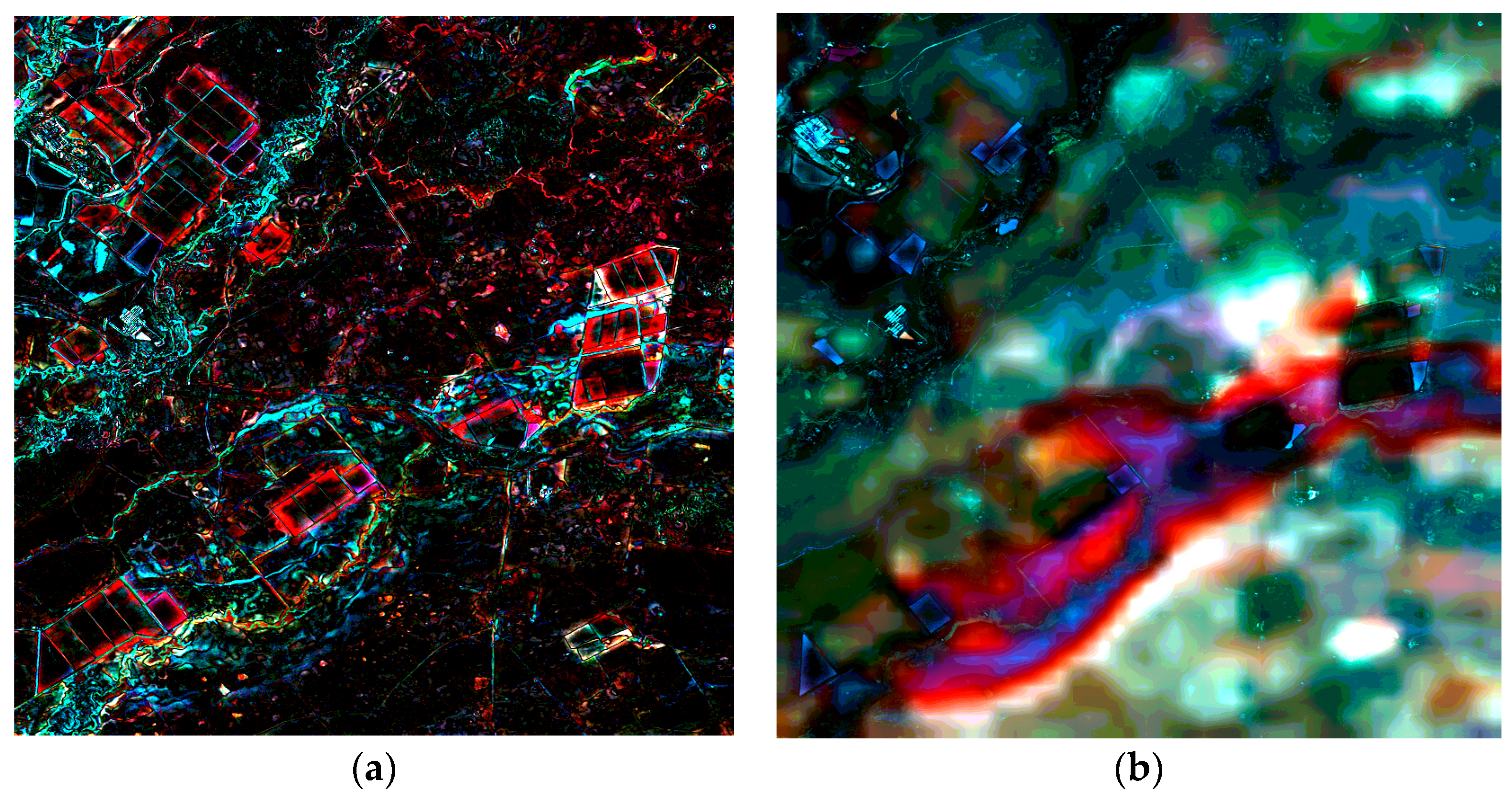
Figure 10 shows the squared error (Figure 10a) and estimation variance (Figure 10b) results of the fusion image predicted using the RWSTFM. Some overlapping areas can still be detected in the squared error and estimation variance maps, especially for inundated areas. The estimation variance map has a global, but discrepant value distribution. The edges of changed areas have high estimation variances. From Figure 6b, Figure 8b and Figure 10b, we can summarize that the shapes and edges of surface objects show higher uncertainties because the heterogeneous areas around the edges have less coincident similar pixels. In contrast, homogeneous areas with a denser distribution of similar pixels and unchanged land cover areas have lower uncertainties. The overall characteristics of the uncertainties in the fusion predictions are likely to be determined by the similar pixels used for training, the specific parameters of the ordinary kriging method and the land surface reflectance change during the observation periods. First, the prediction uncertainty is determined by both the densities and variabilities of similar pixels in the neighborhood of the prediction location [47]. Generally, pixel locations with more coincident variations and denser similar pixels in the neighborhood will have lower prediction uncertainties [48]. Additionally, the prediction uncertainty is affected by the specific parameters of ordinary kriging method employed, e.g., variogram function and nugget model [49,50]. In this paper, we have employed an ordinary kriging method based on geostatistical assumptions. We assume that the observed data are stationary for spectrally similar pixels within a local window. Additionally, we have applied a variogram function to fit the relationship between the semivariance and distance from known sample points and an extra nugget model to capture the nugget effect. Finally, larger surface reflectance changes lead to larger uncertainties in the fusion results as a result of differences in the land surface reflectance between two observation dates.
Table 6 shows percentages of 84.79%, 85.31% and 85.11% for the three bands. The ratios of all three of the datasets are higher than 0.7, which proves that the prediction uncertainty can effectively describe the prediction error. Hence, the RWSTFM can provide an estimate of the prediction error variance (i.e., a measurement of the local uncertainty) and produce some internal estimates of the prediction precision.
5. Conclusions
This paper has proposed a novel geostatistical fusion method, namely RWSTFM, to blend Landsat and MODIS images and obtain prediction uncertainties that could simultaneously help users to estimate the credibility of fusion results. We tested the RWSTFM method on three datasets for New South Wales and compared its performance with that of the STARFM and FSDAF methods. The experimental results show that the RWSTFM model performed better than the other two methods in terms of both a visual comparison and a quantitative evaluation. Additionally, the squared error covered by the estimation variance accounted for more than 70% among all three of the datasets. In contrast, the STARFM experienced difficulties in predicting land cover changes and preserving spatial details, especially within heterogeneous areas. Although the FSDAF method performed better than the STARFM for the second dataset with land cover change, it still produced some spectral confusion along adjacent boundaries with similar spectra distributed on either side and smoothed the trivial inner details of the same end-members in heterogeneous coarse-resolution pixels. Both the STARFM and FSDAF methods adopt an ad hoc weighted function for the fusion prediction and residual distribution process. Unlike these two spatiotemporal methods, the RWSTFM derives the weights in terms of the fitted semivariance-distance relationship using spectrally similar neighboring pixels. It can also predict both changed and unchanged land cover areas uniformly. Furthermore, the RWSTFM searches for spectrally similar pixels by considering the structural similarity for the changed areas such that the amplitudes and structures of changes can be captured more precisely. These capabilities thus enable the RWSTFM method to outperform the STARFM and FSDAF methods, particularly with regard to delineating and characterizing the changes. Remarkably, the RWSTFM provides an estimation variance, which can be used as a measure of the prediction uncertainty. Such a capability is not available within STARFM, the FSDAF method or any other fusion method.
However, our method could still be improved in several aspects. First, change information cannot be precisely detected from MODIS images, especially with regard to producing spatial details that are not indicated within coarse-resolution images on the prediction date. This is a highly challenging task that may be conducted using spectrally similar pixels to exactly locate reflectance changes. This aspect will be addressed more precisely in our research. Second, we adopt a simple threshold to detect the changes in the surface reflectance images at different dates. It could be improved by establishing the histogram of the absolute difference maps for calculating the corresponding thresholds. Third, the parameter of the search window size is determined by the homogeneity of the surface. The search window size could be automatically selected in our future work. Furthermore, performing the local weighted method by kriging and finding spectrally similar pixels in changed areas are time consuming. The processing time is mainly determined by the size of the data site and the search window size. We perform our method RWSTFM by MATLAB programming in a desktop with an Intel i5 3.2-GHz processor, 8 GB RAM and a 1 TB hard disk. For Datasets 1 and 2 with a size of 480 × 480 × 3, it will consume almost an hour. For Dataset 3 with a size of 800 × 800 × 3, it will consume about 3 h. If we assume the time spent on calculating the kriging weights of every pixel is a constant, the complexity of this program is O(), where b is the number of bands and is the size of the image. However, as we know, the processing time is also determined by land cover changed area and searching time of spectrally similar pixels, which is related to the image size. This problem can be resolved by improving computer performance or utilizing parallel computing.
Acknowledgments
This study was jointly supported by the National Natural Science Foundation of China (Grant No.: A.03.14.00901) and Hong Kong Research Grants Council under GRF (Grant No.: 14652016). Thanks to the anonymous reviewers and the editor for their constructive comments and helpful suggestions, which have greatly improved this manuscript.
Author Contributions
Bo Huang conceived and designed the experiments; Jing Wang performed the experiments; Jing Wang and Bo Huang analyzed the data; Jing Wang and Bo Huang wrote the paper.
Conflicts of Interest
The authors declare no conflict of interest.
References
- Markham, B.L.; Storey, J.C.; Williams, D.L.; Irons, J.R. Landsat sensor performance: History and current status. IEEE Trans. Geosci. Remote Sens. 2004, 42, 2691–2694. [Google Scholar] [CrossRef]
- Lansing, J.C. The Landsat Sensors Status, Application, and Plans. J. Imaging Technol. 1987, 13, 191–195. [Google Scholar]
- Barnes, W.L.; Pagano, T.S.; Salomonson, V.V. Prelaunch characteristics of the Moderate Resolution Imaging Spectroradiometer (MODIS) on EOS-AM1. IEEE Trans. Geosci. Remote Sens. 1998, 36, 1088–1100. [Google Scholar] [CrossRef]
- Justice, C.O.; Townshend, J.R.G.; Vermote, E.F.; Masuoka, E.; Wolfe, R.E.; Saleous, N.; Roy, D.P.; Morisette, J.T. An overview of MODIS Land data processing and product status. Remote Sens. Environ. 2002, 83, 3–15. [Google Scholar] [CrossRef]
- Jia, K.; Liang, S.L.; Wei, X.Q.; Yao, Y.J.; Su, Y.R.; Jiang, B.; Wang, X.X. Land Cover Classification of Landsat Data with Phenological Features Extracted from Time Series MODIS NDVI Data. Remote Sens. 2014, 6, 11518–11532. [Google Scholar] [CrossRef]
- Walker, J.; de Beurs, K.; Wynne, R. Phenological Response of an Arizona Dryland Forest to Short-Term Climatic Extremes. Remote Sens. 2015, 7, 10832–10855. [Google Scholar] [CrossRef]
- Zhang, B.H.; Zhang, L.; Xie, D.; Yin, X.L.; Liu, C.J.; Liu, G. Application of Synthetic NDVI Time Series Blended from Landsat and MODIS Data for Grassland Biomass Estimation. Remote Sens. 2016, 8, 10. [Google Scholar] [CrossRef]
- Knauer, K.; Gessner, U.; Fensholt, R.; Kuenzer, C. An ESTARFM Fusion Framework for the Generation of Large-Scale Time Series in Cloud-Prone and Heterogeneous Landscapes. Remote Sens. 2016, 8, 425. [Google Scholar] [CrossRef]
- Huang, B.; Zhang, H.K.; Song, H.H.; Wang, J.; Song, C.Q. Unified fusion of remote-sensing imagery: Generating simultaneously high-resolution synthetic spatialtemporalspectral earth observations. Remote Sens. Lett. 2013, 4, 561–569. [Google Scholar] [CrossRef]
- Addesso, P.; Longo, M.; Restaino, R.; Vivone, G. Sequential Bayesian Methods for Resolution Enhancement of TIR Image Sequences. IEEE J. Sel. Top. Appl. Earth Obs. Remote Sens. 2015, 8, 233–243. [Google Scholar] [CrossRef]
- Mercier, G.; Hubert-Moy, L.; Houet, T.; Gouery, P. Estimation and monitoring of bare soil/vegetation ratio with SPOT VEGETATION and HRVIR. IEEE Trans. Geosci. Remote Sens. 2005, 43, 348–354. [Google Scholar] [CrossRef]
- Moosavi, V.; Talebi, A.; Mokhtari, M.H.; Shamsi, S.R.F.; Niazi, Y. A wavelet-artificial intelligence fusion approach (WAIFA) for blending Landsat and MODIS surface temperature. Remote Sens. Environ. 2015, 169, 243–254. [Google Scholar] [CrossRef]
- Laporterie-Dejean, F.; Flouzat, G.; Lopez-Ornelas, E. Multitemporal and multiresolution fusion of wide field of view and high spatial resolution images through morphological pyramid. Image Signal Process. Remote Sens. 2004, 5573, 52–63. [Google Scholar]
- Roy, D.P.; Ju, J.; Lewis, P.; Schaaf, C.; Gao, F.; Hansen, M.; Lindquist, E. Multi-temporal MODIS–Landsat data fusion for relative radiometric normalization, gap filling, and prediction of Landsat data. Remote Sens. Environ. 2008, 112, 3112–3130. [Google Scholar] [CrossRef]
- Gao, F.; Masek, J.; Schwaller, M.; Hall, F. On the blending of the Landsat and MODIS surface reflectance: Predicting daily Landsat surface reflectance. IEEE Trans. Geosci. Remote Sens. 2006, 44, 2207–2218. [Google Scholar]
- Hilker, T.; Wulder, M.A.; Coops, N.C.; Linke, J.; McDermid, G.; Masek, J.G.; Gao, F.; White, J.C. A new data fusion model for high spatial- and temporal-resolution mapping of forest disturbance based on Landsat and MODIS. Remote Sens. Environ. 2009, 113, 1613–1627. [Google Scholar] [CrossRef]
- Zhu, X.; Chen, J.; Gao, F.; Chen, X.; Masek, J.G. An enhanced spatial and temporal adaptive reflectance fusion model for complex heterogeneous regions. Remote Sens. Environ. 2010, 114, 2610–2623. [Google Scholar] [CrossRef]
- Zhukov, B.; Oertel, D.; Lanzl, F.; Reinhackel, G. Unmixing-based multisensor multiresolution image fusion. IEEE Trans. Geosci. Remote Sens. 1999, 37, 1212–1226. [Google Scholar] [CrossRef]
- Zhang, W.; Li, A.N.; Jin, H.A.; Bian, J.H.; Zhang, Z.J.; Lei, G.B.; Qin, Z.H.; Huang, C.Q. An Enhanced Spatial and Temporal Data Fusion Model for Fusing Landsat and MODIS Surface Reflectance to Generate High Temporal Landsat-Like Data. Remote Sens. 2013, 5, 5346–5368. [Google Scholar] [CrossRef]
- Bai, Y.; Wong, M.S.; Shi, W.Z.; Wu, L.X.; Qin, K. Advancing of Land Surface Temperature Retrieval Using Extreme Learning Machine and Spatio-Temporal Adaptive Data Fusion Algorithm. Remote Sens. 2015, 7, 4424–4441. [Google Scholar] [CrossRef]
- Rao, Y.H.; Zhu, X.L.; Chen, J.; Wang, J.M. An Improved Method for Producing High Spatial-Resolution NDVI Time Series Datasets with Multi-Temporal MODIS NDVI Data and Landsat TM/ETM plus Images. Remote Sens. 2015, 7, 7865–7891. [Google Scholar] [CrossRef]
- Doxani, G.; Mitraka, Z.; Gascon, F.; Goryl, P.; Bojkov, B.R. A Spectral Unmixing Model for the Integration of Multi-Sensor Imagery: A Tool to Generate Consistent Time Series Data. Remote Sens. 2015, 7, 14000–14018. [Google Scholar] [CrossRef]
- Amorós-López, J.; Gómez-Chova, L.; Alonso, L.; Guanter, L.; Zurita-Milla, R.; Moreno, J.; Camps-Valls, G. Multitemporal fusion of Landsat/TM and ENVISAT/MERIS for crop monitoring. Int. J. Appl. Earth Obs. Geoinf. 2013, 23, 132–141. [Google Scholar] [CrossRef]
- Huang, B.; Zhang, H. Spatio-temporal reflectance fusion via unmixing: Accounting for both phenological and land-cover changes. Int. J. Remote Sens. 2014, 35, 6213–6233. [Google Scholar] [CrossRef]
- Wu, M.; Wu, C.; Huang, W.; Niu, Z.; Wang, C.; Li, W.; Hao, P. An improved high spatial and temporal data fusion approach for combining Landsat and MODIS data to generate daily synthetic Landsat imagery. Inf. Fusion 2016, 31, 14–25. [Google Scholar] [CrossRef]
- Wu, M.Q.; Niu, Z.; Wang, C.Y.; Wu, C.Y.; Wang, L. Use of MODIS and Landsat time series data to generate high-resolution temporal synthetic Landsat data using a spatial and temporal reflectance fusion model. J. Appl. Remote Sens. 2012, 6. [Google Scholar] [CrossRef]
- Zhu, X.L.; Helmer, E.H.; Gao, F.; Liu, D.S.; Chen, J.; Lefsky, M.A. A flexible spatiotemporal method for fusing satellite images with different resolutions. Remote Sens. Environ. 2016, 172, 165–177. [Google Scholar] [CrossRef]
- Huang, B.; Song, H.H. Spatiotemporal Reflectance Fusion via Sparse Representation. IEEE Trans. Geosci. Remote Sens. 2012, 50, 3707–3716. [Google Scholar] [CrossRef]
- Song, H.H.; Huang, B. Spatiotemporal Satellite Image Fusion Through One-Pair Image Learning. IEEE Trans. Geosci. Remote Sens. 2013, 51, 1883–1896. [Google Scholar] [CrossRef]
- Wu, B.; Huang, B.; Zhang, L.P. An Error-Bound-Regularized Sparse Coding for Spatiotemporal Reflectance Fusion. IEEE Trans. Geosci. Remote Sens. 2015, 53, 6791–6803. [Google Scholar] [CrossRef]
- Matheron, G. Kriging or Polynomial Interpolation Procedures—A Contribution to Polemics in Mathematical Geology. Can. Min. Metall. Bull. 1967, 60, 240–244. [Google Scholar]
- Odeh, I.O.A.; Mcbratney, A.B.; Chittleborough, D.J. Further Results on Prediction of Soil Properties from Terrain Attributes—Heterotopic Cokriging and Regression-Kriging. Geoderma 1995, 67, 215–226. [Google Scholar] [CrossRef]
- Jeffrey, S.J.; Carter, J.O.; Moodie, K.B.; Beswick, A.R. Using spatial interpolation to construct a comprehensive archive of Australian climate data. Environ. Model. Softw. 2001, 16, 309–330. [Google Scholar] [CrossRef]
- Haylock, M.R.; Hofstra, N.; Tank, A.M.G.K.; Klok, E.J.; Jones, P.D.; New, M. A European daily high-resolution gridded dataset of surface temperature and precipitation for 1950–2006. J. Geophys. Res. Atmos. 2008, 113. [Google Scholar] [CrossRef]
- Pardo-Iguzquiza, E.; Rodriguez-Galiano, V.F.; Chica-Olmo, M.; Atkinson, P.M. Image fusion by spatially adaptive filtering using downscaling cokriging. ISPRS J. Photogramm. Remote Sens. 2011, 66, 337–346. [Google Scholar] [CrossRef]
- Sales, M.H.R.; Souza, C.M.; Kyriakidis, P.C. Fusion of MODIS Images Using Kriging With External Drift. IEEE Trans. Geosci. Remote Sens. 2013, 51, 2250–2259. [Google Scholar] [CrossRef]
- Wang, Q.M.; Shi, W.Z.; Atkinson, P.M.; Pardo-Iguquiza, E. A New Geostatistical Solution to Remote Sensing Image Downscaling. IEEE Trans. Geosci. Remote Sens. 2016, 54, 386–396. [Google Scholar] [CrossRef]
- Wang, Q.M.; Shi, W.Z.; Li, Z.B.; Atkinson, P.M. Fusion of Sentinel-2 images. Remote Sens. Environ. 2016, 187, 241–252. [Google Scholar] [CrossRef]
- Yamamoto, J.K. An alternative measure of the reliability of ordinary kriging estimates. Math. Geol. 2000, 32, 489–509. [Google Scholar] [CrossRef]
- Lloyd, C.D.; Atkinson, P.M. Assessing uncertainty in estimates with ordinary and indicator kriging. Comput. Geosci. 2001, 27, 929–937. [Google Scholar] [CrossRef]
- Vicente-Serrano, S.M.; Perez-Cabello, F.; Lasanta, T. Assessment of radiometric correction techniques in analyzing vegetation variability and change using time series of Landsat images. Remote Sens. Environ. 2008, 112, 3916–3934. [Google Scholar] [CrossRef]
- Krige, D.G. Longterm Trends in Domestic Metal Prices under International Conditions of Differential Inflation Rates and Unstable Currency Exchange-Rates. J. S. Afr. Inst. Min. Metall. 1978, 79, 42–49. [Google Scholar]
- Van der Meer, F. Remote-sensing image analysis and geostatistics. Int. J. Remote Sens. 2012, 33, 5644–5676. [Google Scholar] [CrossRef]
- Srivastava, R.M.; Isaaks, E.H. An Introduction to Applied Geostatistics; Oxford University Press: New York, NY, USA, 1989; 561p. [Google Scholar]
- Wald, L. Data Fusion: Definitions and Architectures—Fusion of Images of Different Spatial Resolutions; Les Presses, Ecole des Mines de Paris: Paris, France, 2002. [Google Scholar]
- Emelyanova, I.V.; McVicar, T.R.; Van Niel, T.G.; Li, L.T.; van Dijk, A.I.J.M. Assessing the accuracy of blending Landsat-MODIS surface reflectances in two landscapes with contrasting spatial and temporal dynamics: A framework for algorithm selection. Remote Sens. Environ. 2013, 133, 193–209. [Google Scholar] [CrossRef]
- Stein, A.; Bastiaanssen, W.G.M.; De Bruin, S.; Cracknell, A.P.; Curran, P.J.; Fabbri, A.G.; Gorte, B.G.H.; Van Groenigen, J.W.; Van der Meer, F.D.; Saldana, A. Integrating spatial statistics and remote sensing. Int. J. Remote Sens. 1998, 19, 1793–1814. [Google Scholar] [CrossRef]
- Goovaerts, P. Geostatistics in soil science: State-of-the-art and perspectives. Geoderma 1999, 89, 1–45. [Google Scholar] [CrossRef]
- Mcbratney, A.B.; Webster, R. Choosing Functions for Semi-Variograms of Soil Properties and Fitting Them to Sampling Estimates. J. Soil Sci. 1986, 37, 617–639. [Google Scholar] [CrossRef]
- Atkinson, P.M. Downscaling in remote sensing. Int. J. Appl. Earth Obs. Geoinf. 2013, 22, 106–114. [Google Scholar] [CrossRef]
Figure 1.
Flowchart of the rigorously-weighted spatiotemporal fusion model (RWSTFM) for blending Landsat and MODIS imagery.
Figure 1.
Flowchart of the rigorously-weighted spatiotemporal fusion model (RWSTFM) for blending Landsat and MODIS imagery.

Figure 2.
The first dataset exhibiting phenological changes: NIR-red-green composites of the Landsat images with a 30-m spatial resolution from (a) 2 May 2004 and (b) 5 July 2004; the corresponding MODIS images with a 500-m spatial resolution from (c) 2 May 2004 and (d) 5 July 2004.
Figure 2.
The first dataset exhibiting phenological changes: NIR-red-green composites of the Landsat images with a 30-m spatial resolution from (a) 2 May 2004 and (b) 5 July 2004; the corresponding MODIS images with a 500-m spatial resolution from (c) 2 May 2004 and (d) 5 July 2004.

Figure 3.
The second dataset exhibiting land cover changes: NIR-red-green composites of the Landsat images with a 30-m spatial resolution from (a) 26 November 2004 and (b) 28 December 2004; the corresponding MODIS images with a 500-m spatial resolution from (c) 26 November 2004 and (d) 28 December 2004.
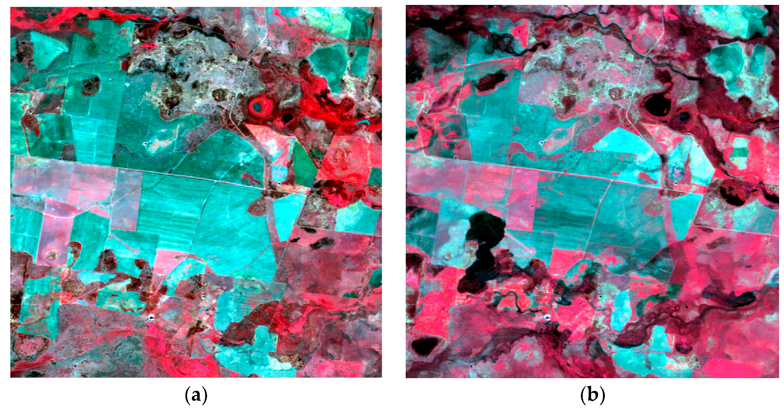
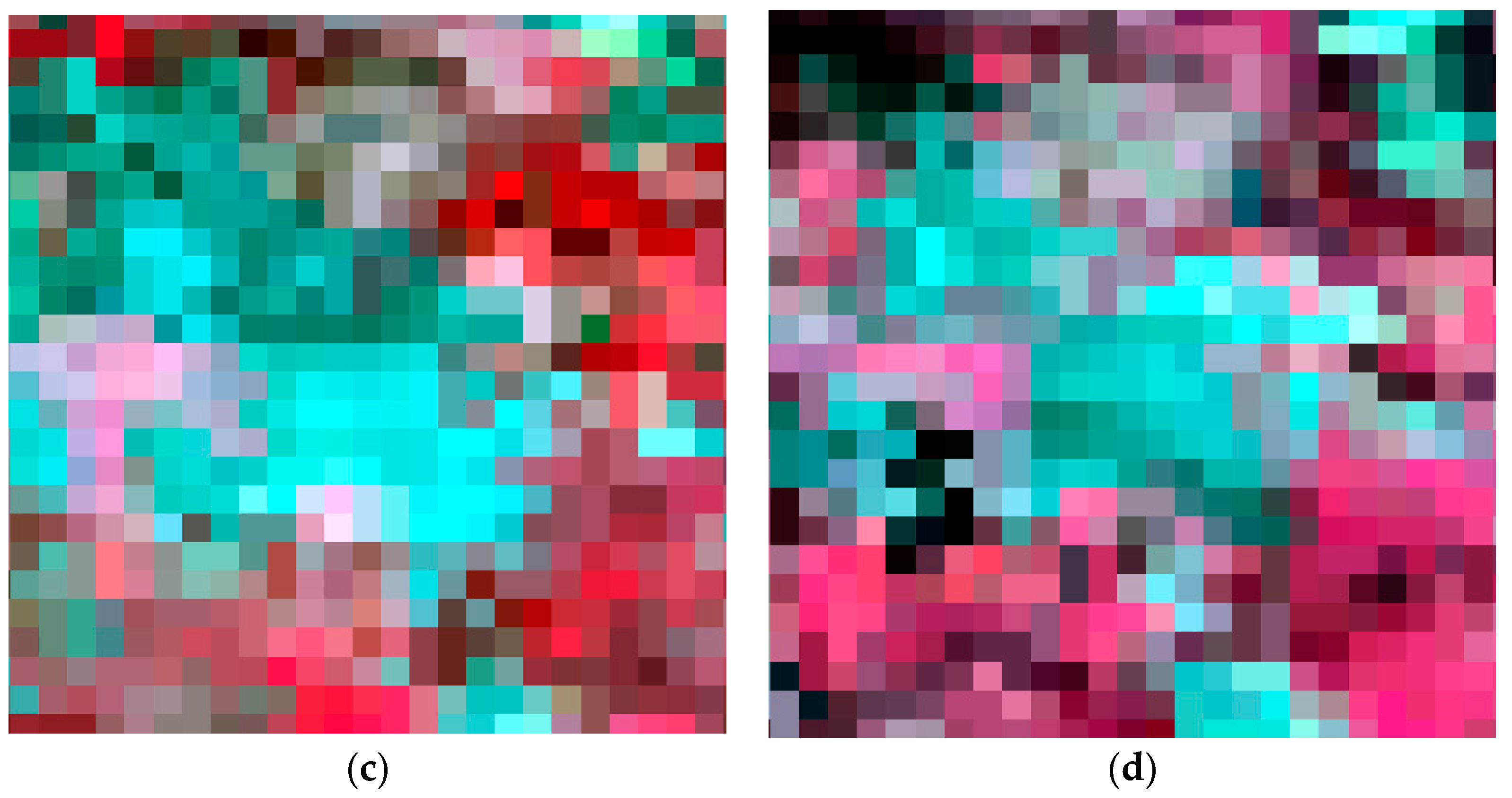
Figure 4.
The dataset exhibiting both phenological and land cover changes: NIR-red-green composites of the Landsat images with a 30-m spatial resolution from (a) 25 October 2004 and (b) 12 December 2004; the corresponding MODIS images with a 500-m spatial resolution from (c) 25 October 2004 and (d) 12 December 2004.
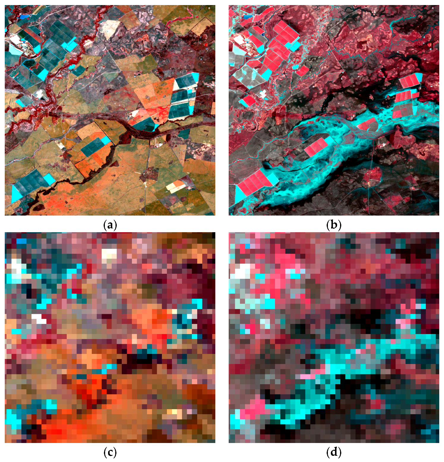
Figure 5.
Comparison of the fusion results from the spatial and temporal adaptive reflectance fusion model (STARFM), flexible spatiotemporal data fusion (FSDAF) and RWSTFM methods for the first dataset: NIR-red-green composites of (a) the original Landsat image from 5 July 2004; (b) the predicted image using the STARFM; (c) the predicted image using the FSDAF; and (d) the predicted image using the RWSTFM.
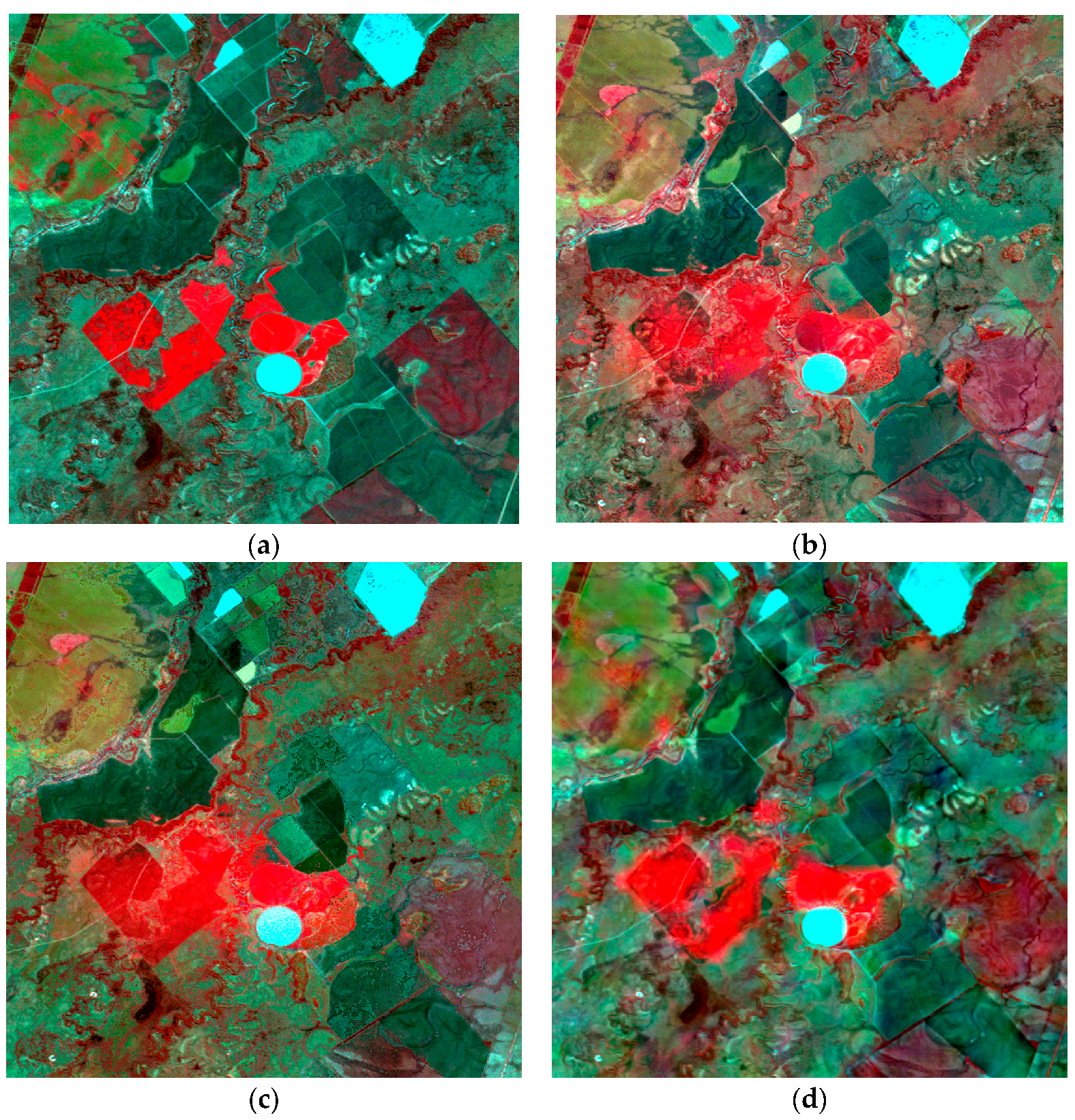
Figure 6.
NIR-red-green composites of the squared error (with max values for bands NIR, red and green are 0.0030, 0.0006 and 0.0005) (a) and estimation variance (with max values for bands NIR, red and green are 0.0029, 0.0009 and 0.0007); (b) results for the first dataset.
Figure 6.
NIR-red-green composites of the squared error (with max values for bands NIR, red and green are 0.0030, 0.0006 and 0.0005) (a) and estimation variance (with max values for bands NIR, red and green are 0.0029, 0.0009 and 0.0007); (b) results for the first dataset.

Figure 7.
Comparison of the fusion results from the STARFM, FSDAF and RWSTFM methods for the second dataset: NIR-red-green composites of (a) the original Landsat image from 28 December 2004; (b) the predicted image using the STARFM; (c) the predicted image using the FSDAF; and (d) the predicted image using the RWSTFM.
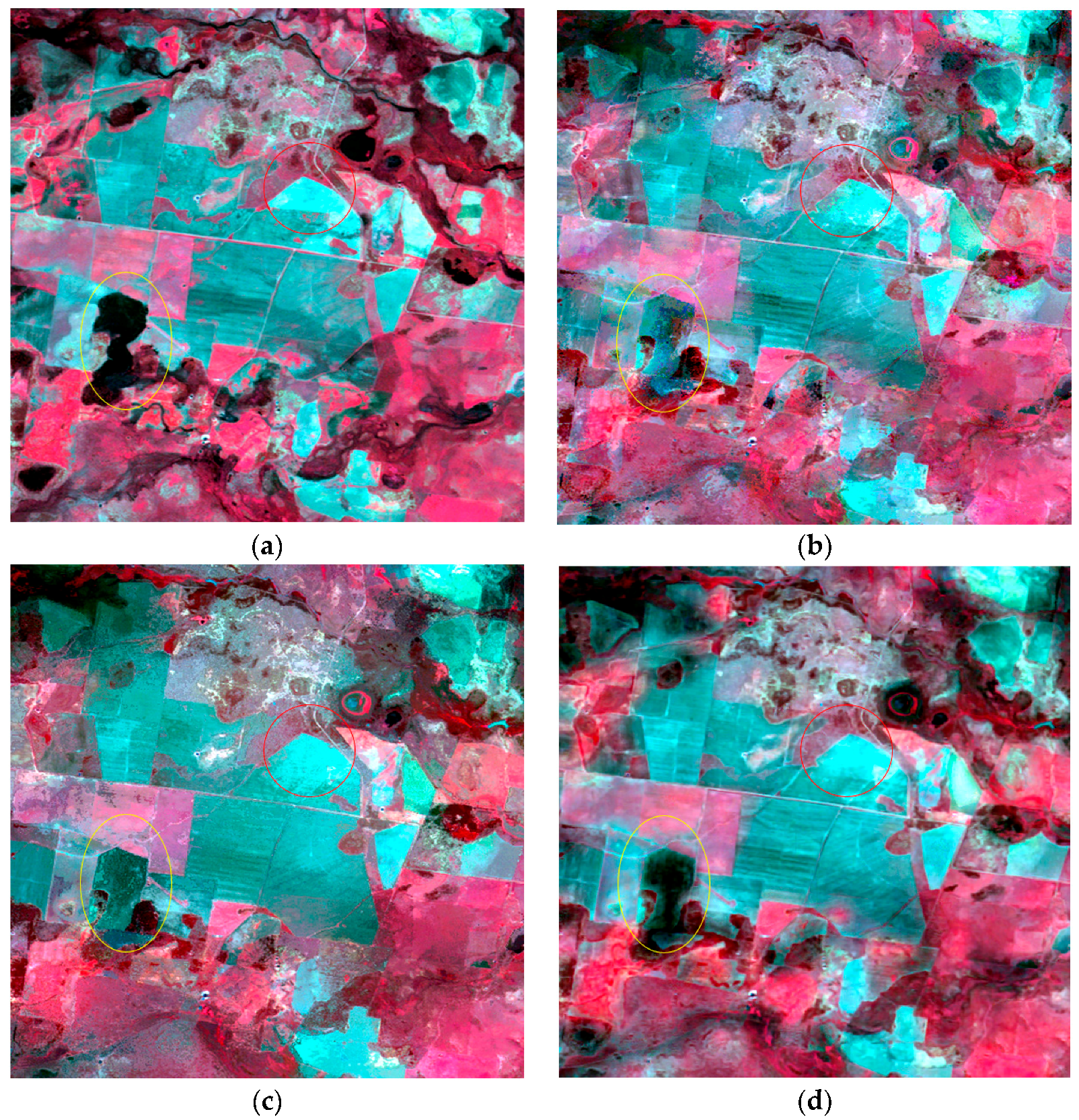
Figure 8.
NIR-red-green composites of the squared error (with max values for bands NIR, red and green are 0.0023, 0.0002 and 0.0002) (a) and estimation variance (with max values for bands NIR, red and green are 0.0019, 0.0008 and 0.0005); (b) results for the second dataset.
Figure 8.
NIR-red-green composites of the squared error (with max values for bands NIR, red and green are 0.0023, 0.0002 and 0.0002) (a) and estimation variance (with max values for bands NIR, red and green are 0.0019, 0.0008 and 0.0005); (b) results for the second dataset.

Figure 9.
Comparison of the fusion results from the STARFM, FSDAF and RWSTFM methods for the third dataset: NIR-red-green composites of (a) the original Landsat image from 12 December 2004; (b) the predicted image using the STARFM; (c) the predicted image using the FSDAF; and (d) the predicted image using the RWSTFM.
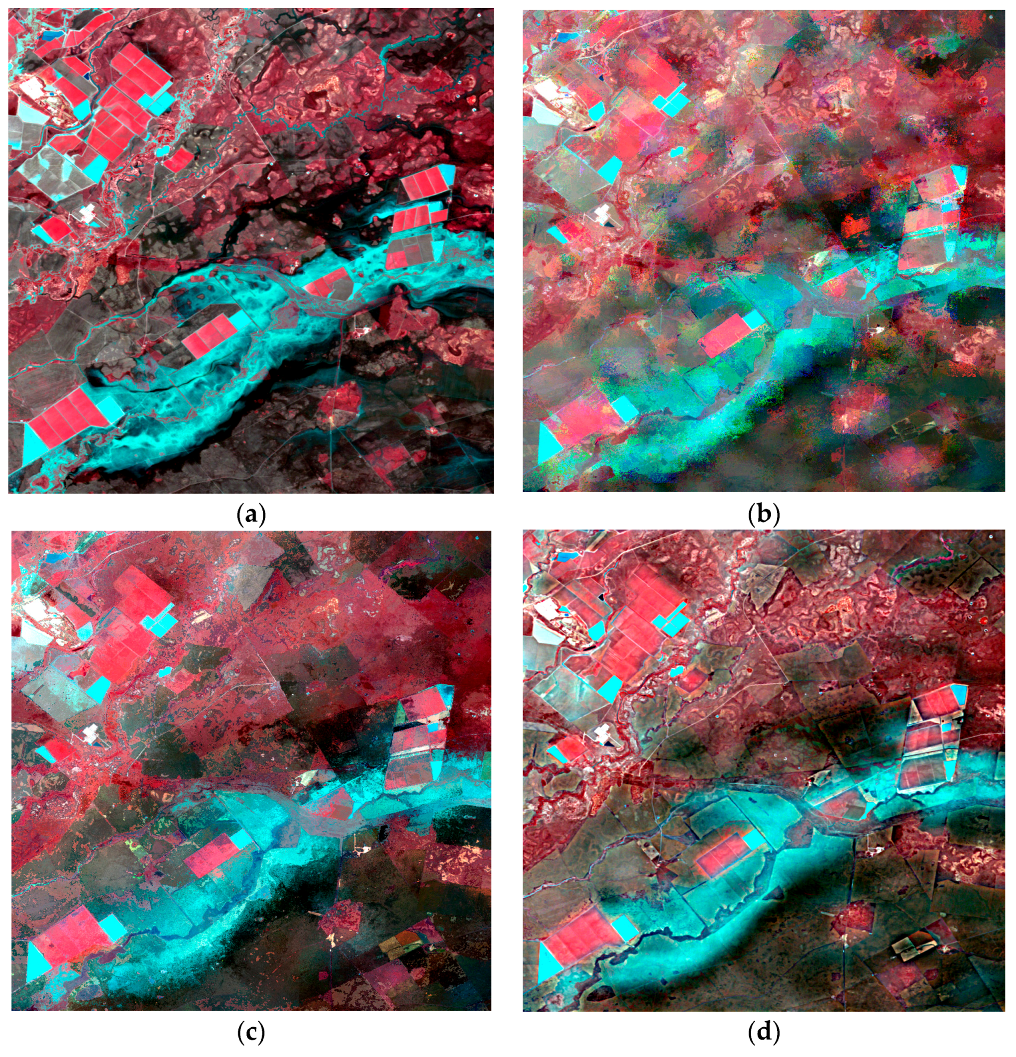
Figure 10.
NIR-red-green composites of the squared error (with max values for bands NIR, red and green are 0.0025, 0.0011, and 0.0007) (a) and estimation variance (with max values for bands NIR, red and green are 0.0013, 0.0011 and 0.0008); (b) results for the third dataset.
Figure 10.
NIR-red-green composites of the squared error (with max values for bands NIR, red and green are 0.0025, 0.0011, and 0.0007) (a) and estimation variance (with max values for bands NIR, red and green are 0.0013, 0.0011 and 0.0008); (b) results for the third dataset.


Table 1.
The fusion results from the STARFM, FSDAF and RWSTFM methods evaluated using objective indices for the first dataset. CC, correlation coefficient; AAD, average absolute difference; AD, average difference; SSIM, structure similarity; ERGAS, erreur relative globale adimensionnelle de synthese.
| Method | STARFM | FSDAF | RWSTFM | |
|---|---|---|---|---|
| RMSE | Band 2 | 0.0026 | 0.0028 | 0.0018 |
| Band 3 | 0.0034 | 0.0035 | 0.0026 | |
| Band 4 | 0.0078 | 0.0076 | 0.0056 | |
| CC | Band 2 | 0.8368 | 0.8331 | 0.8839 |
| Band 3 | 0.8083 | 0.8262 | 0.8726 | |
| Band 4 | 0.7095 | 0.7603 | 0.8228 | |
| AAD | Band 2 | 0.0021 | 0.0023 | 0.0013 |
| Band 3 | 0.0027 | 0.0028 | 0.0018 | |
| Band 4 | 0.0050 | 0.0056 | 0.0032 | |
| AD | Band 2 | −0.0015 | −0.0018 | −0.0003 |
| Band 3 | −0.0015 | −0.0020 | −0.0008 | |
| Band 4 | −0.0038 | −0.0043 | 0.0006 | |
| SSIM | Band 2 | 0.8258 | 0.8102 | 0.8838 |
| Band 3 | 0.7984 | 0.8041 | 0.8719 | |
| Band 4 | 0.6585 | 0.7285 | 0.8204 | |
| ERGAS | 1.4923 | 1.5282 | 1.0814 | |
Table 2.
The percentages of the squared error () that is lower than the estimation variance () for the first dataset.
Table 2.
The percentages of the squared error () that is lower than the estimation variance () for the first dataset.
| Datasets | The First Dataset | ||
|---|---|---|---|
| Bands | Band 2 | Band 3 | Band 4 |
| Percentage (%) | 81.08 | 83.15 | 85.54 |
Table 3.
The fusion results from the STARFM, FSDAF and RWSTFM methods evaluated using objective indices for the second dataset.
Table 3.
The fusion results from the STARFM, FSDAF and RWSTFM methods evaluated using objective indices for the second dataset.
| Method | STARFM | FSDAF | RWSTFM | |
|---|---|---|---|---|
| RMSE | Band 2 | 0.0022 | 0.0021 | 0.0016 |
| Band 3 | 0.0030 | 0.0029 | 0.0021 | |
| Band 4 | 0.0075 | 0.0073 | 0.0056 | |
| CC | Band 2 | 0.7635 | 0.7946 | 0.8889 |
| Band 3 | 0.8012 | 0.8261 | 0.9025 | |
| Band 4 | 0.6921 | 0.7199 | 0.8413 | |
| AAD | Band 2 | 0.0016 | 0.0016 | 0.0012 |
| Band 3 | 0.0023 | 0.0022 | 0.0016 | |
| Band 4 | 0.0053 | 0.0052 | 0.0040 | |
| AD | Band 2 | 0.0001 | −0.0003 | −0.0001 |
| Band 3 | −0.0003 | −0.0007 | −0.0001 | |
| Band 4 | −0.0003 | −0.0009 | −0.0000 | |
| SSIM | Band 2 | 0.7579 | 0.7707 | 0.8834 |
| Band 3 | 0.7982 | 0.8090 | 0.8973 | |
| Band 4 | 0.6598 | 0.6826 | 0.8235 | |
| ERGAS | 1.4399 | 1.3708 | 1.0334 | |
Table 4.
The percentages of the squared error () that is lower than the estimation variance () for the second dataset.
Table 4.
The percentages of the squared error () that is lower than the estimation variance () for the second dataset.
| Datasets | The Second Dataset | ||
|---|---|---|---|
| Bands | Band 2 | Band 3 | Band 4 |
| Percentage (%) | 94.78 | 94.89 | 72.68 |
Table 5.
The fusion results from the STARFM, FSDAF and RWSTFM methods evaluated using objective indices for the third dataset.
Table 5.
The fusion results from the STARFM, FSDAF and RWSTFM methods evaluated using objective indices for the third dataset.
| Method | STARFM | FSDAF | RWSTFM | |
|---|---|---|---|---|
| RMSE | Band 2 | 0.0032 | 0.0030 | 0.0026 |
| Band 3 | 0.0041 | 0.0039 | 0.0035 | |
| Band 4 | 0.0065 | 0.0065 | 0.0060 | |
| CC | Band 2 | 0.7699 | 0.7964 | 0.8604 |
| Band 3 | 0.7482 | 0.7615 | 0.8181 | |
| Band 4 | 0.7437 | 0.7249 | 0.7717 | |
| AAD | Band 2 | 0.0023 | 0.0022 | 0.0018 |
| Band 3 | 0.0028 | 0.0027 | 0.0025 | |
| Band 4 | 0.0045 | 0.0049 | 0.0044 | |
| AD | Band 2 | 0.0002 | 0.0000 | 0.0000 |
| Band 3 | 0.0003 | 0.0000 | 0.0000 | |
| Band 4 | 0.0014 | 0.0002 | 0.0000 | |
| SSIM | Band 2 | 0.7584 | 0.7807 | 0.8582 |
| Band 3 | 0.7422 | 0.7483 | 0.8172 | |
| Band 4 | 0.7393 | 0.7202 | 0.7688 | |
| ERGAS | 1.7734 | 1.8159 | 1.5449 | |
Table 6.
The percentages of the squared error () that is lower than the estimation variance () for the third dataset.
Table 6.
The percentages of the squared error () that is lower than the estimation variance () for the third dataset.
| Datasets | The Third Dataset | ||
|---|---|---|---|
| Bands | Band 2 | Band 3 | Band 4 |
| Percentage (%) | 84.79 | 85.31 | 85.11 |
© 2017 by the authors. Licensee MDPI, Basel, Switzerland. This article is an open access article distributed under the terms and conditions of the Creative Commons Attribution (CC BY) license (http://creativecommons.org/licenses/by/4.0/).
Share and Cite
MDPI and ACS Style
Wang, J.; Huang, B. A Rigorously-Weighted Spatiotemporal Fusion Model with Uncertainty Analysis. Remote Sens. 2017, 9, 990. https://doi.org/10.3390/rs9100990
AMA Style
Wang J, Huang B. A Rigorously-Weighted Spatiotemporal Fusion Model with Uncertainty Analysis. Remote Sensing. 2017; 9(10):990. https://doi.org/10.3390/rs9100990
Chicago/Turabian StyleWang, Jing, and Bo Huang. 2017. "A Rigorously-Weighted Spatiotemporal Fusion Model with Uncertainty Analysis" Remote Sensing 9, no. 10: 990. https://doi.org/10.3390/rs9100990
Note that from the first issue of 2016, this journal uses article numbers instead of page numbers. See further details here.