Spectro-Temporal Heterogeneity Measures from Dense High Spatial Resolution Satellite Image Time Series: Application to Grassland Species Diversity Estimation


Abstract
:
1. Introduction
2. Materials
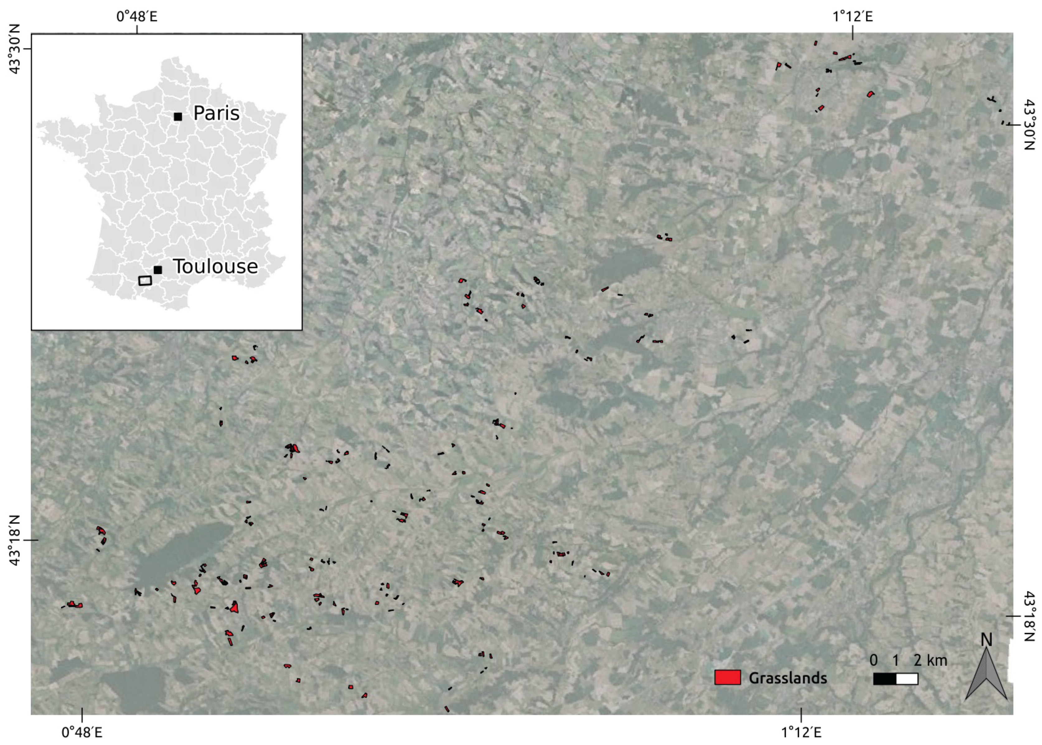
2.1. Study Area
2.2. Satellite Image Time Series
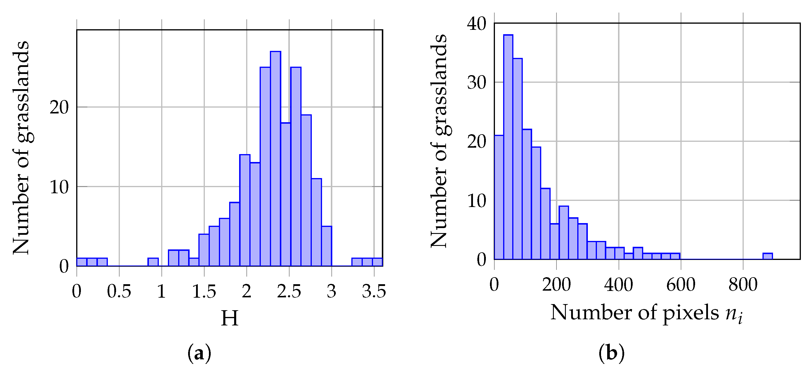
2.3. Field Data
3. Method
3.1. Measures of Spectral Heterogeneity in the Literature
3.2. Spectral Clustering Algorithm for High Dimensional Data and Derived Measures of Spectral Heterogeneity
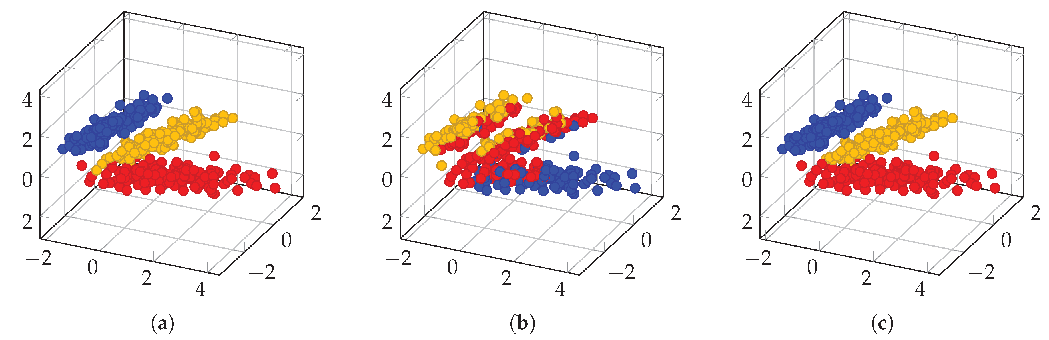
3.2.1. Between- and Within-Class Variabilities
- is the between-class covariance matrix,
- is the spectro-temporal mean of pixels in assigned to cluster c,
- is the mean spectro-temporal value computed from all the pixels of ,
- is the within-class covariance matrix,
- is the empirical covariance matrix of pixels of assigned to cluster c.
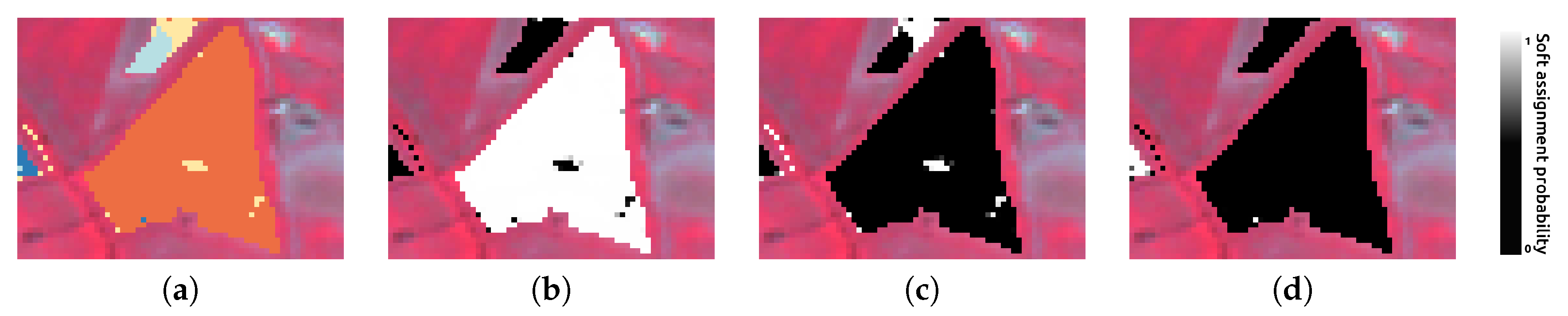
3.2.2. Entropy
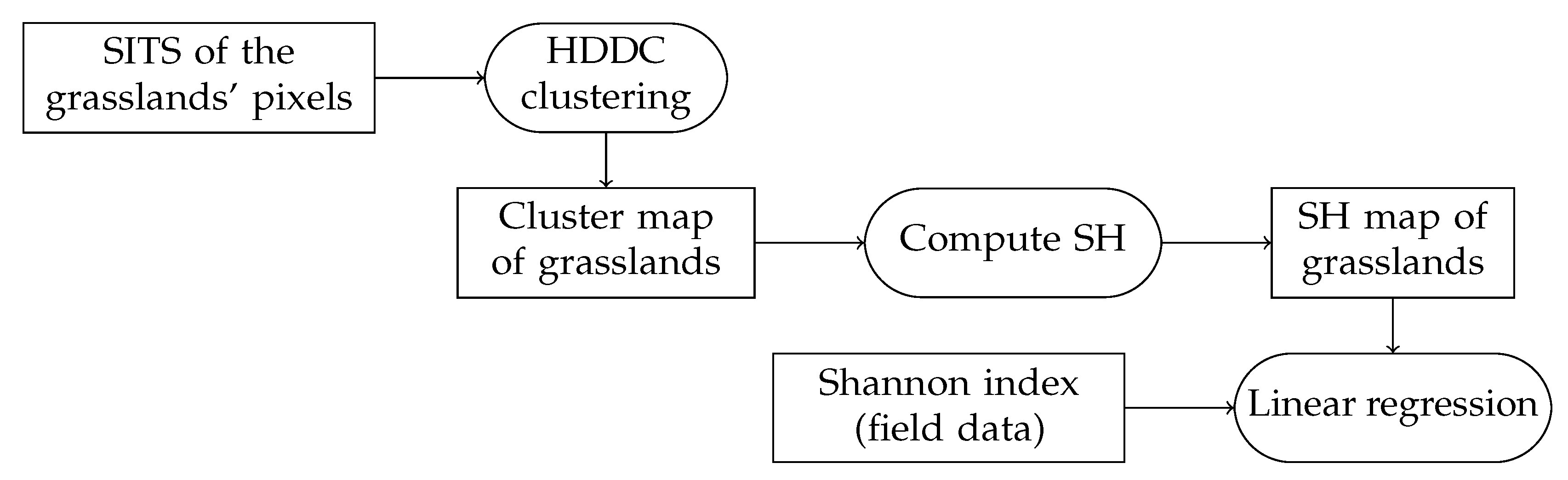
3.3. Methodology
4. Results
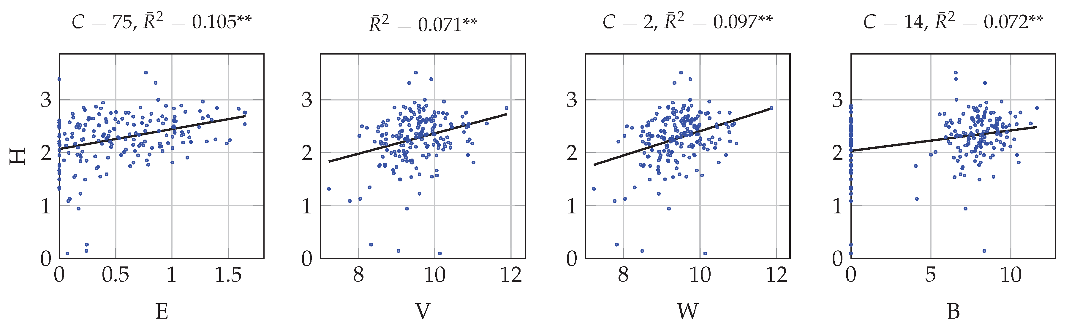
4.1. Univariate Correlation with Multitemporal Data
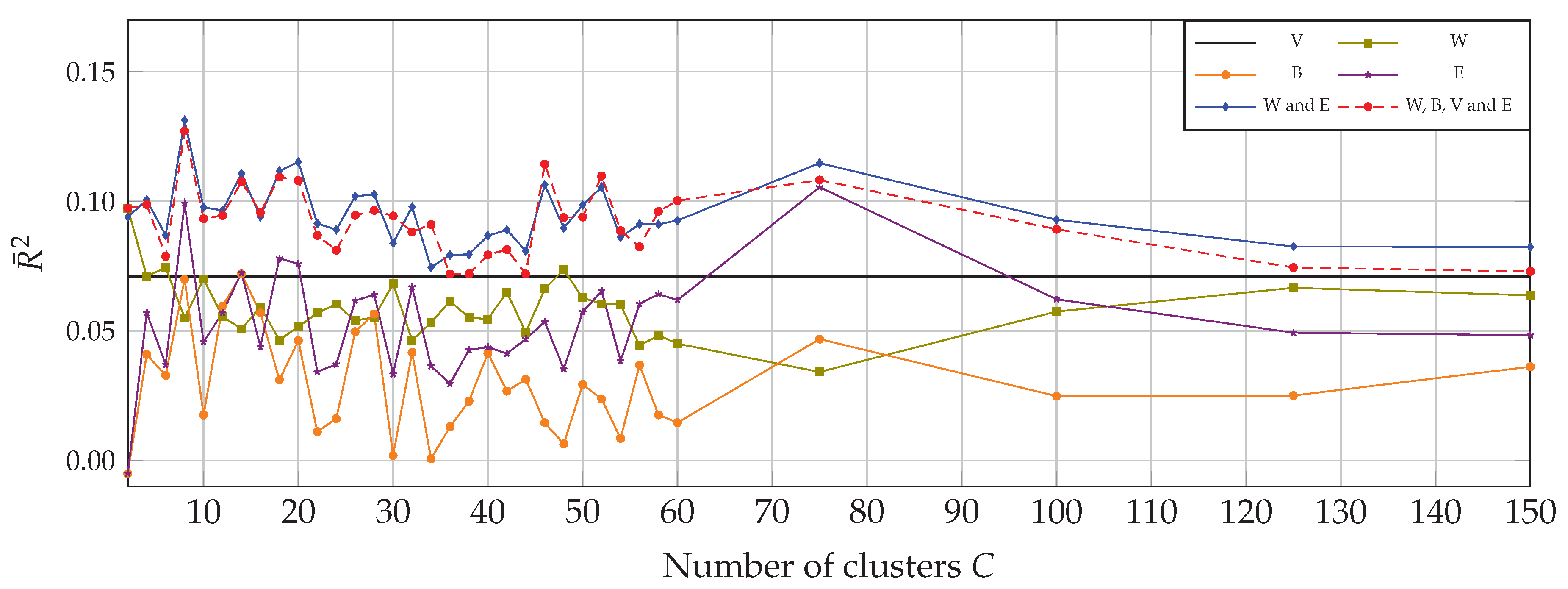
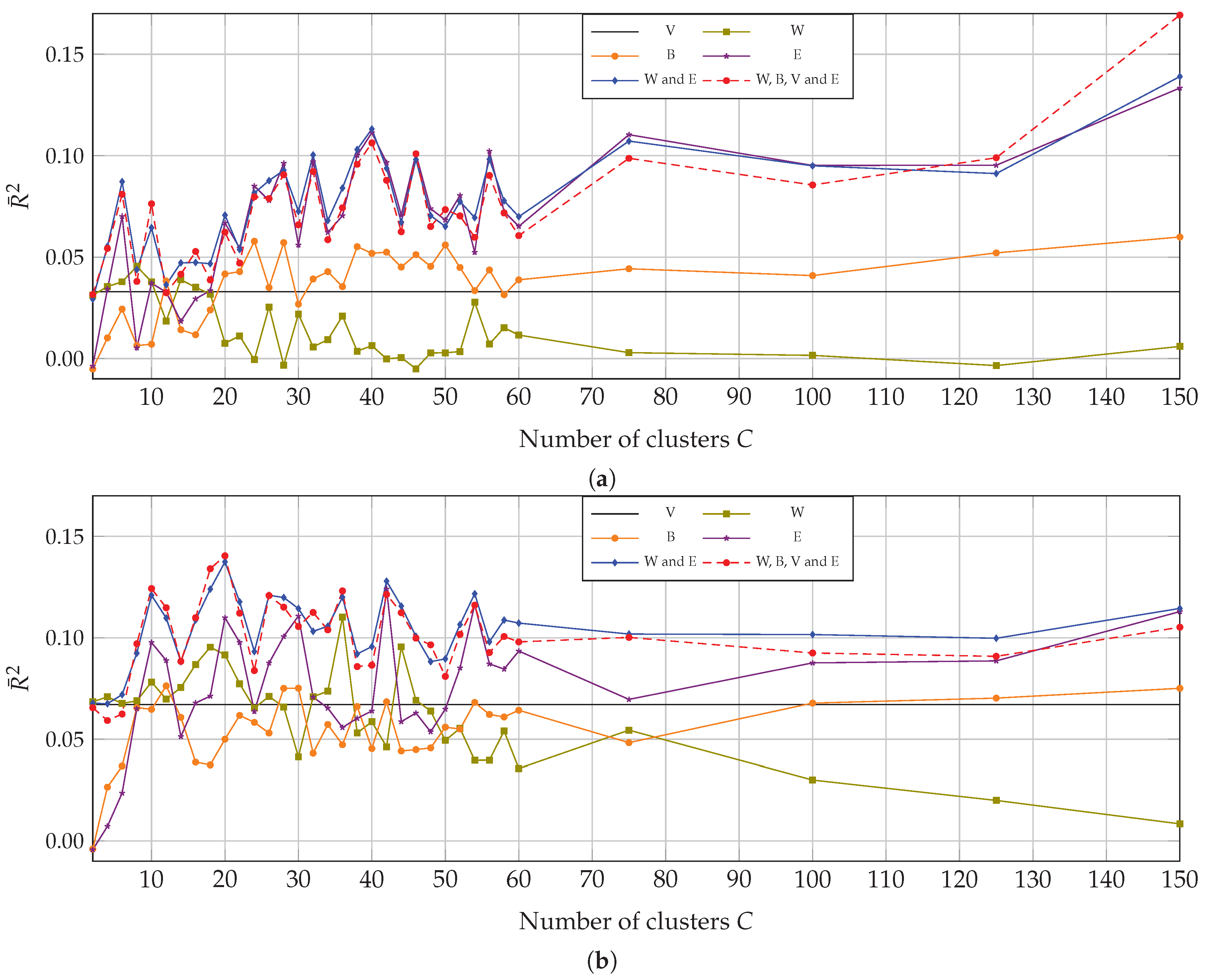
4.2. Multivariate Correlation with Multitemporal Data
4.3. Univariate and Multivariate Correlation with Monotemporal Data
5. Discussion
5.1. Spectral Heterogeneity Measures
5.2. Clustering
5.3. Contribution of Multitemporal Imagery
5.4. Limitations
5.5. Outlooks
6. Conclusions
Acknowledgments
Author Contributions
Conflicts of Interest
Abbreviations
| B | Log-transformed between-classes variability |
| CNES | Centre National d’Etudes Spatiales (French spatial agency) |
| E | Entropy computed from soft assignment |
| GIS | Geographic Information System |
| H | Shannon index |
| HDDC | High Dimensional Discriminant Clustering |
| ICL | Integrated Classification Likelihood |
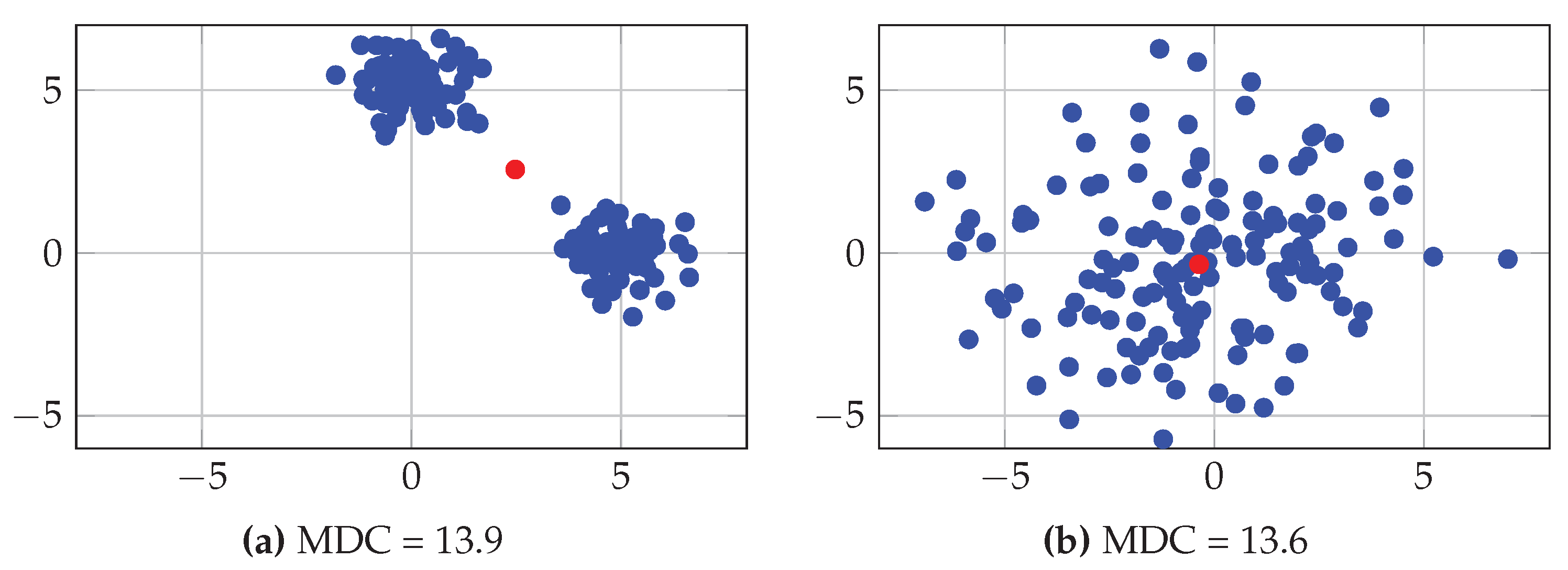
| MDC | Mean Distance to Centroid |
| NDVI | Normalized Difference Vegetation Index |
| NIR | Near-Infrared |
| PCA | Principal Components Analysis |
| SH | Spectral Heterogeneity |
| SITS | Satellite Image Time Series |
| STVH | Spectro-Temporal Variation Hypothesis |
| SVH | Spectral Variation Hypothesis |
| V | Log-transformed global variability |
| W | Log-transformed within-class variability |
Appendix A

| Species | a | b | c |
|---|---|---|---|
| Agrimonia eupatoria | + | ||
| Agrostis capillaris | 1 | ||
| Anthoxanthum odoratum | 1 | ||
| Arrhenatherum elatius | 1 | ||
| Bellis perennis | 1 | ||
| Bromus erectus | 1 | ||
| Carex divulsa | + | ||
| Carex flacca | 1 | ||
| Centaurea nigra | + | ||
| Cirsium arvense | 1 | ||
| Cirsium dissectum | 1 | ||
| Cirsium vulgare | + | ||
| Convolvulus arvensis | 1 | 1 | |
| Crepis capillaris | 1 | ||
| Crepis spp. | + | ||
| Dactylis glomerata | 1 | 3 | |
| Daucus carota | 1 | ||
| Festuca arundinacea | 2 | 3 | |
| Festuca rubra | 1 | ||
| Galium mollugo | 1 | ||
| Gaudinia fragilis | 1 | ||
| Holcus lanatus | 1 | ||
| Hypericum perforatum | + | ||
| Hypochaeris radicata | 1 | 1 | |
| Lathyrus pratensis | 2 | ||
| Leucanthemum vulgare | 1 | ||
| Linum usitatissimum | 1 | ||
| Lolium perenne | 5 | ||
| Lotus corniculatus | 1 | ||
| Medicago spp. | + | ||
| Muscari comosum | + | ||
| Orchis purpurea | + | ||
| Plantago lanceolata | 1 | ||
| Poa pratensis | 2 | ||
| Poa trivialis | + | 5 | |
| Potentilla reptans | 1 | 1 | |
| Prunus spinosa | 1 | ||
| Rafanus spp. | + | ||
| Ranunculus acris | 1 | ||
| Ranunculus bulbosus | 1 | ||
| Ranunculus repens | 2 | ||
| Rasica oleacera | + | ||
| Rhinanthus minor | + | ||
| Rubus spp. | + | ||
| Rumex acetosa | 1 | ||
| Rumex crispus | 1 | + | |
| Senecio jacobaea | 1 | ||
| Sonchus asper | + | ||
| Stachys officinalis | + | ||
| Taraxacum officinalis | 1 1 | ||
| Tragopogon pratensis | + + | ||
| Trifolium dubium | 2 | ||
| Trifolium pratense | 1 | 2 | |
| Trifolium repens | 1 | ||
| Verbena officinalis | 1 | ||
| Veronica arvensis | + | ||
| Veronica arvensis | + | ||
| Vicia sativa | + | 1 |
References
- Eriksson, A.; Eriksson, O.; Berglund, H. Species Abundance Patterns of Plants in Swedish Semi-Natural Pastures. Ecography 1995, 18, 310–317. [Google Scholar] [CrossRef]
- Critchley, C.; Burke, M.; Stevens, D. Conservation of lowland semi-natural grasslands in the UK: A review of botanical monitoring results from agri-environment schemes. Biol. Conserv. 2004, 115, 263–278. [Google Scholar] [CrossRef]
- O’Mara, F.P. The role of grasslands in food security and climate change. Anna. Bot. 2012, 110, 1263–1270. [Google Scholar] [CrossRef] [PubMed]
- Werling, B.P.; Dickson, T.L.; Isaacs, R.; Gaines, H.; Gratton, C.; Gross, K.L.; Liere, H.; Malmstrom, C.M.; Meehan, T.D.; Ruan, L.; et al. Perennial grasslands enhance biodiversity and multiple ecosystem services in bioenergy landscapes. Proc. Natl. Acad. Sci. USA 2014, 111, 1652–1657. [Google Scholar] [CrossRef] [PubMed]
- Magurran, A. Ecological Diversity and Its Measurement; Croom Helm: Kent, UK, 1988. [Google Scholar]
- Shannon, C.E. A Mathematical Theory of Communication. Bell Syst. Tech. J. 1948, 27, 379–423. [Google Scholar] [CrossRef]
- Simpson, E.H. Measurement of diversity. Nature 1949, 163, 688. [Google Scholar] [CrossRef]
- Rocchini, D.; Balkenhol, N.; Carter, G.A.; Foody, G.M.; Gillespie, T.W.; He, K.S.; Kark, S.; Levin, N.; Lucas, K.; Luoto, M.; et al. Remotely sensed spectral heterogeneity as a proxy of species diversity: Recent advances and open challenges. Ecol. Inform. 2010, 5, 318–329. [Google Scholar] [CrossRef]
- Skidmore, A.K.; Pettorelli, N.; Coops, N.C.; Geller, G.N.; Hansen, M.; Lucas, R.; Mücher, C.A.; O’Connor, B.; Paganini, M.; Pereira, H.M.; et al. Environmental science: Agree on biodiversity metrics to track from space. Nature 2015, 523, 403–405. [Google Scholar] [CrossRef] [PubMed]
- Rocchini, D.; Boyd, D.S.; Féret, J.B.; Foody, G.M.; He, K.S.; Lausch, A.; Nagendra, H.; Wegmann, M.; Pettorelli, N. Satellite remote sensing to monitor species diversity: Potential and pitfalls. Remote Sens. Ecol. Conserv. 2016, 2, 25–36. [Google Scholar] [CrossRef]
- Pettorelli, N.; Laurance, W.F.; O’Brien, T.G.; Wegmann, M.; Nagendra, H.; Turner, W. Satellite remote sensing for applied ecologists: Opportunities and challenges. J. Appl. Ecol. 2014, 51, 839–848. [Google Scholar] [CrossRef]
- Cord, A.F.; Brauman, K.A.; Chaplin-Kramer, R.; Huth, A.; Ziv, G.; Seppelt, R. Priorities to Advance Monitoring of Ecosystem Services Using Earth Observation. Trends Ecol. Evol. 2017, 32, 416–428. [Google Scholar] [CrossRef] [PubMed]
- Kerr, J.T.; Ostrovsky, M. From space to species: Ecological applications for remote sensing. Trends Ecol. Evol. 2003, 18, 299–305. [Google Scholar] [CrossRef]
- Gould, W. Remote Sensing of Vegetation, Plant Species Richness, and Regional Biodiversity Hotspots. Ecol. Appl. 2000, 10, 1861–1870. [Google Scholar] [CrossRef]
- Palmer, M.W.; Earls, P.G.; Hoagland, B.W.; White, P.S.; Wohlgemuth, T. Quantitative tools for perfecting species lists. Environmetrics 2002, 13, 121–137. [Google Scholar] [CrossRef]
- Wilson, J.; Fuller, S.J.; Mather, P.B. Formation and maintenance of discrete wild rabbit (Oryctolagus cuniculus) population systems in arid Australia: Habitat heterogeneity and management implications. Austral Ecol. 2002, 27, 183–191. [Google Scholar] [CrossRef]
- Tews, J.; Brose, U.; Grimm, V.; Tielbörger, K.; Wichmann, M.C.; Schwager, M.; Jeltsch, F. Animal species diversity driven by habitat heterogeneity/diversity: The importance of keystone structures. J. Biogeogr. 2004, 31, 79–92. [Google Scholar] [CrossRef]
- Oldeland, J.; Wesuls, D.; Rocchini, D.; Schmidt, M.; Jürgens, N. Does using species abundance data improve estimates of species diversity from remotely sensed spectral heterogeneity? Ecol. Indic. 2010, 10, 390–396. [Google Scholar] [CrossRef]
- Möckel, T.; Dalmayne, J.; Schmid, B.C.; Prentice, H.C.; Hall, K. Airborne Hyperspectral Data Predict Fine-Scale Plant Species Diversity in Grazed Dry Grasslands. Remote Sens. 2016, 8, 133. [Google Scholar]
- Oindo, B.O.; Skidmore, A.K. Interannual variability of NDVI and species richness in Kenya. Int. J. Remote Sens. 2002, 23, 285–298. [Google Scholar] [CrossRef]
- Fairbanks, D.H.K.; McGwire, K.C. Patterns of Floristic Richness in Vegetation Communities of California: Regional Scale Analysis with Multi-Temporal NDVI. Glob. Ecol. Biogeogr. 2004, 13, 221–235. [Google Scholar] [CrossRef]
- Rocchini, D. Effects of spatial and spectral resolution in estimating ecosystem α-diversity by satellite imagery. Remote Sens. Environ. 2007, 111, 423–434. [Google Scholar] [CrossRef]
- Féret, J.B.; Asner, G.P. Mapping tropical forest canopy diversity using high-fidelity imaging spectroscopy. Ecol. Appl. 2014, 24, 1289–1296. [Google Scholar] [CrossRef]
- Drusch, M.; Bello, U.D.; Carlier, S.; Colin, O.; Fernandez, V.; Gascon, F.; Hoersch, B.; Isola, C.; Laberinti, P.; Martimort, P.; et al. Sentinel-2: ESA’s Optical High-Resolution Mission for GMES Operational Services. Remote Sens. Environ. 2012, 120, 25–36. [Google Scholar] [CrossRef]
- Hooper, D.U. The role of complementarity and competition in ecosystem responses to variation in plant diversity. Ecology 1998, 79, 704–719. [Google Scholar] [CrossRef]
- Sakai, S. Phenological diversity in tropical forests. Popul. Ecol. 2001, 43, 77–86. [Google Scholar] [CrossRef]
- Ryschawy, J.; Choisis, N.; Choisis, J.P.; Joannon, A.; Gibon, A. Mixed crop-livestock systems: An economic and environmental-friendly way of farming? Animal 2012, 6, 1722–1730. [Google Scholar] [CrossRef] [PubMed]
- Carrié, R.; Andrieu, E.; Cunningham, S.A.; Lentini, P.E.; Loreau, M.; Ouin, A. Relationships among ecological traits of wild bee communities along gradients of habitat amount and fragmentation. Ecography 2017, 40, 85–97. [Google Scholar] [CrossRef]
- Hagolle, O.; Huc, M.; Villa Pascual, D.; Dedieu, G. A multi-temporal method for cloud detection, applied to FORMOSAT-2, VENuS, LANDSAT and SENTINEL-2 images. Remote Sens. Environ. 2010, 114, 1747–1755. [Google Scholar] [CrossRef] [Green Version]
- Eilers, P.H.C. A Perfect Smoother. Anal. Chem. 2003, 75, 3631–3636. [Google Scholar] [CrossRef] [PubMed]
- Atzberger, C.; Eilers, P.H.C. Evaluating the effectiveness of smoothing algorithms in the absence of ground reference measurements. Int. J. Remote Sens. 2011, 32, 3689–3709. [Google Scholar] [CrossRef]
- Braun-Blanquet, J.; Fuller, G.; Conard, H. Plant Sociology: The Study of Plant Communities: Authorized English Translation of Pflanzensoziologie; McGraw-Hill Publications in the Botanical Sciences; McGraw-Hill: New York, NY, USA, 1932. [Google Scholar]
- Parsons, L.; Haque, E.; Liu, H. Subspace Clustering for High Dimensional Data: A Review. Acm Sigkdd Explor. Newsl. 2004, 6, 90–105. [Google Scholar] [CrossRef]
- Bouveyron, C.; Girard, S.; Schmid, C. High-dimensional data clustering. Comput. Stat. Data Anal. 2007, 52, 502–519. [Google Scholar] [CrossRef]
- Lagrange, A.; Fauvel, M.; Grizonnet, M. Large-Scale Feature Selection with Gaussian Mixture Models for the Classification of High Dimensional Remote Sensing Images. IEEE Trans. Comput. Imaging 2017, 3, 230–242. [Google Scholar] [CrossRef]
- Bouveyron, C.; Girard, S.; Schmid, C. High-Dimensional Discriminant Analysis. Commun. Stat. Theory Methods 2007, 36, 2607–2623. [Google Scholar] [CrossRef]
- Girard, S.; Saracco, J. Supervised and Unsupervised Classification Using Mixture Models. EAS Publ. Ser. 2016, 77, 69–90. [Google Scholar] [CrossRef]
- Neyrinck, M.C.; Szapudi, I.; Szalay, A.S. Rejuvenating the Matter Power Spectrum: Restoring Information with a Logarithmic Density Mapping. Astrophys. J. Lett. 2009, 698, L90. [Google Scholar] [CrossRef]
- Hall, K.; Reitalu, T.; Sykes, M.T.; Prentice, H.C. Spectral heterogeneity of QuickBird satellite data is related to fine-scale plant species spatial turnover in semi-natural grasslands. Appl. Veg. Sci. 2012, 15, 145–157. [Google Scholar] [CrossRef]
- Pedregosa, F.; Varoquaux, G.; Gramfort, A.; Michel, V.; Thirion, B.; Grisel, O.; Blondel, M.; Prettenhofer, P.; Weiss, R.; Dubourg, V.; et al. Scikit-learn: Machine Learning in Python. J. Mach. Learn. Res. 2011, 12, 2825–2830. [Google Scholar]
- Biernacki, C.; Celeux, G.; Govaert, G. Assessing a Mixture Model for Clustering with the Integrated Completed Likelihood. IEEE Trans. Pattern Anal. Mach. Intell. 2000, 22, 719–725. [Google Scholar] [CrossRef]
- Price, J.C. How unique are spectral signatures? Remote Sens. Environ. 1994, 49, 181–186. [Google Scholar] [CrossRef]
- Nagendra, H. Using remote sensing to assess biodiversity. Int. J. Remote Sens. 2001, 22, 2377–2400. [Google Scholar] [CrossRef]
- Moog, D.; Poschlod, P.; Kahmen, S.; Schreiber, K.F. Comparison of species composition between different grassland management treatments after 25 years. Appl. Veg. Sci. 2002, 5, 99–106. [Google Scholar] [CrossRef]
- Schäfer, E.; Heiskanen, J.; Heikinheimo, V.; Pellikka, P. Mapping tree species diversity of a tropical montane forest by unsupervised clustering of airborne imaging spectroscopy data. Ecol. Indic. 2016, 64, 49–58. [Google Scholar] [CrossRef]
- Maeda, E.E.; Heiskanen, J.; Thijs, K.W.; Pellikka, P.K. Season-dependence of remote sensing indicators of tree species diversity. Remote Sens. Lett. 2014, 5, 404–412. [Google Scholar] [CrossRef]
- Pärtel, M.; Zobel, M. Small-scale plant species richness in calcareous grasslands determined by the species pool, community age and shoot density. Ecography 1999, 22, 153–159. [Google Scholar] [CrossRef]
- Bruun, H.H. Patterns of Species Richness in Dry Grassland Patches in an Agricultural Landscape. Ecography 2000, 23, 641–650. [Google Scholar] [CrossRef]
- Franzén, D.; Eriksson, O. Small-scale patterns of species richness in Swedish semi-natural grasslands: The effects of community species pools. Ecography 2001, 24, 505–510. [Google Scholar] [CrossRef]
- Bray, J.R.; Curtis, J.T. An Ordination of the Upland Forest Communities of Southern Wisconsin. Ecol. Monogr. 1957, 27, 325–349. [Google Scholar] [CrossRef]
- Ustin, S.L.; Gamon, J.A. Remote sensing of plant functional types. New Phytol. 2010, 186, 795–816. [Google Scholar] [CrossRef] [PubMed]
- Homolová, L.; Malenovský, Z.; Clevers, J.G.; García-Santos, G.; Schaepman, M.E. Review of optical-based remote sensing for plant trait mapping. Ecol. Complex. 2013, 15, 1–16. [Google Scholar] [CrossRef]
- Jetz, W.; Cavender-Bares, J.; Pavlick, R.; Schimel, D.; Davis, F.W.; Asner, G.P.; Guralnick, R.; Kattge, J.; Latimer, A.M.; Moorcroft, P.; et al. Monitoring plant functional diversity from space. Nature Plants 2016, 2, 1–5. [Google Scholar] [CrossRef] [PubMed]
- Abelleira Martínez, O.J.; Fremier, A.K.; Günter, S.; Ramos Bendaña, Z.; Vierling, L.; Galbraith, S.M.; Bosque-Pérez, N.A.; Ordoñez, J.C. Scaling up functional traits for ecosystem services with remote sensing: concepts and methods. Ecol. Evol. 2016, 6, 4359–4371. [Google Scholar] [CrossRef] [PubMed]


| Pixel Size | 10 m |
|---|---|
| Spectral bands | B1 “Green” (500–590 nm) |
| B2 “Red” (610–680 nm) | |
| B3 “Near-Infrared” (780–890 nm) | |
| B4 “Short Wave Infrared” (1580–1750 nm) | |
| Acquisition dates | 20-04-2015, 25-04-2015, 30-04-2015, 10-05-2015, 20-05-2015, 04-06-2015, |
| 24-06-2015, 29-06-2015, 04-07-2015, 09-07-2015, 14-07-2015, 19-07-2015, | |
| 24-07-2015, 13-08-2015, 18-08-2015, 28-08-2015, 02-09-2015, 07-09-2015 |
| Response Variable | Explanatory Variables | Reg. Coeff. | Std Err. | p-Value |
|---|---|---|---|---|
| H | W | 0.29 | 0.14 | 0.04 |
| B | 0.01 | 0.02 | 0.61 | |
| V | −0.15 | 0.14 | 0.30 | |
| E | 0.40 | 0.13 | 0.003 | |
| intercept | 0.73 | 0.51 | 0.16 | |
| Model summary: = 8.0, p-value <0.001, = 0.145, | ||||
| H | W | 0.16 | 0.06 | 0.005 |
| E | 0.37 | 0.09 | <0.001 | |
| intercept | 0.65 | 0.51 | 0.20 | |
| Model summary: = 15.4, p-value <0.001, = 0.140, | ||||
© 2017 by the authors. Licensee MDPI, Basel, Switzerland. This article is an open access article distributed under the terms and conditions of the Creative Commons Attribution (CC BY) license (http://creativecommons.org/licenses/by/4.0/).
Share and Cite
Lopes, M.; Fauvel, M.; Ouin, A.; Girard, S. Spectro-Temporal Heterogeneity Measures from Dense High Spatial Resolution Satellite Image Time Series: Application to Grassland Species Diversity Estimation. Remote Sens. 2017, 9, 993. https://doi.org/10.3390/rs9100993
Lopes M, Fauvel M, Ouin A, Girard S. Spectro-Temporal Heterogeneity Measures from Dense High Spatial Resolution Satellite Image Time Series: Application to Grassland Species Diversity Estimation. Remote Sensing. 2017; 9(10):993. https://doi.org/10.3390/rs9100993
Chicago/Turabian StyleLopes, Mailys, Mathieu Fauvel, Annie Ouin, and Stéphane Girard. 2017. "Spectro-Temporal Heterogeneity Measures from Dense High Spatial Resolution Satellite Image Time Series: Application to Grassland Species Diversity Estimation" Remote Sensing 9, no. 10: 993. https://doi.org/10.3390/rs9100993