Submesoscale Sea Surface Temperature Variability from UAV and Satellite Measurements


1
Colorado Center for Astrodynamics Research, University of Colorado, 431 UCB, Boulder, CO 80309, USA
2
NOAA Earth System Research Laboratory, Physical Sciences Division, R/PSD2 325 Broadway, Boulder, CO 80305, USA
3
Ball Aerospace, 1600 Commerce St., Boulder, CO 80301, USA
*
Author to whom correspondence should be addressed.
Remote Sens. 2017, 9(11), 1089; https://doi.org/10.3390/rs9111089
Submission received: 24 September 2017
/
Revised: 17 October 2017
/
Accepted: 23 October 2017
/
Published: 25 October 2017
(This article belongs to the Special Issue Sea Surface Temperature Retrievals from Remote Sensing)
Abstract
:Earlier studies of spatial variability in sea surface temperature (SST) using ship-based radiometric data suggested that variability at scales smaller than 1 km is significant and affects the perceived uncertainty of satellite-derived SSTs. Here, we compare data from the Ball Experimental Sea Surface Temperature (BESST) thermal infrared radiometer flown over the Arctic Ocean against coincident Moderate Resolution Imaging Spectroradiometer (MODIS) measurements to assess the spatial variability of skin SSTs within 1-km pixels. By taking the standard deviation, σ, of the BESST measurements within individual MODIS pixels, we show that significant spatial variability of the skin temperature exists. The distribution of the surface variability measured by BESST shows a peak value of O(0.1) K, with 95% of the pixels showing σ < 0.45 K. Significantly, high-variability pixels are located at density fronts in the marginal ice zone, which are a primary source of submesoscale intermittency near the surface. SST wavenumber spectra indicate a spectral slope of −2, which is consistent with the presence of submesoscale processes at the ocean surface. Furthermore, the BESST wavenumber spectra not only match the energy distribution of MODIS SST spectra at the satellite-resolved wavelengths, they also span the spectral slope of −2 by ~3 decades, from wavelengths of 8 km to <0.08 km.

1. Introduction
Increased spatial resolution in observations of the upper ocean has revealed an abundance of processes on lateral scales of O(1) km (e.g., Thomas et al. [1]). These processes, termed submesoscale, are vital for the transfer of energy from the mesoscale (10–100 km) to the small, three-dimensional processes at scales less than a kilometer (0.1–100 m). While processes at the large and small length scales have been studied extensively, the intermediate scales are less well understood, partly because limitations on instrumental sampling and computational resolution have hindered their research [1]. However, technological advances in the last decade mean that we are now able to achieve the required resolution in models and observations to capture this scale. Submesoscale variability is seen in high-resolution velocity fields from radar [2], sea surface temperature (SST) fields from high-resolution satellites [3], ice-tethered profiler measurements under ice in the Arctic Ocean [4], and hydrographic surveys from towed vehicles and gliders, just to name a few.
Increased scientific understanding has been enabled by the improvements in instrumentation and computational models, and has also established that submesoscale processes play an important role in the vertical transport and mixing of properties and tracers between the surface mixed layer and the thermocline. Submesoscale instabilities are shown to cause rapid changes (they operate on temporal scales spanning from hours to days) in the stratification and buoyancy transport of the mixed layer that cannot be explained by heating and cooling alone, and far exceed what can be achieved through mesoscale baroclinic instability [5,6,7].
An important question is the role that the submesoscale processes play in this transfer of energy from the meso to the small scales where the energy dissipation takes place [8]. The quasi two-dimensional mesoscale flow field is characterized by kinetic energy spectra with a slope of −3. Three-dimensional numerical simulations at progressively finer resolutions show that resolving submesoscale processes leads to the flattening of the kinetic energy spectra slope to −2 [9]. An aspect of relevance for this investigation is that submesoscales are known to be a source of spatial heterogeneity, or patchiness, at the ocean surface. This heterogeneity, or variance of the spatial distribution of properties and tracers (the SST is considered a passive tracer), is caused either by vertical advection at vertical gradients, or by horizontal stirring (lateral gradients at scales of O(1) km that enhance lateral mixing), which promotes surface filamentation. Numerical experiments [1] show that, in the former case, submesoscale processes accelerate vertical stratification (sharper gradients, higher fluxes), introduce submesoscale concentration anomalies at the surface, and shift the spatial variance towards larger scales [10]. In the latter case, the vertical restratification of the surface layer slows down (weaker stratification and fluxes), stretching and stirring tracer filaments at the surface and increasing submesoscale spatial variance at smaller length scales [11].
Here, we present evidence that a substantial portion of the variance of satellite SST products with 1-km spatial resolution resides in the submesoscale range. It is common practice to treat the satellite-retrieved SST at a pixel as a point value, even though the measurement integrates the radiation coming from the surrounding area within the satellite footprint. There is an inherent uncertainty (estimation error) stemming from this representation, as spatial variability is always present in nature. The variance of the SST distribution within the pixel is referred to as the sub-pixel spatial variability. If the variance within the pixel is small, the point value is a good representation of the overall pixel, but as the variance increases, as in frontal regions and coastal and high-latitude regions, the estimation error also increases. This sub-pixel variability can, therefore, contribute to the estimated uncertainty of a satellite-derived SST retrieval when it is validated against an observation with a finer spatial resolution. Another factor contributing to the uncertainty in satellite SST products is the error arising from the discretization of the sampling, as satellite SST products are typically binned (gridded) in some form. A full description of the uncertainty budget of satellite SSTs can be found in Cornillon et al. [12] and the role of subpixel variability as it applies to Cornillon et al. [12] is explored in more detail in this paper.
Earlier studies of the spatial variability in SST using ship-based radiometric data suggested that the variability at scales smaller than 1 km is significant and affects the estimated uncertainty of satellite-derived skin SSTs, as derived from the in situ observations. In Castro et al. [13], we showed that, although satellite IR SSTs are more physically related to the ocean skin temperature, a satellite SST regression algorithm trained on subsurface temperatures had better accuracy (less variance) than when the regression coefficients were derived from coincidently measured skin temperatures. This was found by developing and testing parallel skin and subsurface SST regression algorithms using coincident temperatures from both research-grade thermometers and highly accurate radiometers deployed simultaneously from research ships. After comparing the SST variance from both types of algorithms (the subsurface-trained algorithm consistently outperformed the skin-trained algorithm), we concluded that the spatial variability of the skin layer was significantly larger than the variability below the ocean surface. The amount of noise (variability) that needed to be added to the retrieved subsurface temperatures in order to degrade their accuracy to the same level of the skin SSTs was on the order of 0.1–0.17 K. Variogram analysis suggested that differences in both measurement uncertainty and spatial variability with depth contributed equally to the levels of noise needed to produce equal accuracy between the two algorithms (~0.07–0.10 K for each source of uncertainty). A contribution of 0.1 K to the total uncertainty budget is not negligible if one considers that the SST accuracy needed to detect climate change requires that the uncertainties associated with the SST measurement be less than 0.3 K [14]. Contrary to popular belief, the results in Brink and Cowles [15] provide evidence that the radiometric satellite measurement, being a weighted average of the horizontal array of skin temperatures within the footprint and thus less variable than the point measurements from state-of-the-art in situ radiometers, is in better agreement with the smoother subsurface temperatures than to the shipborne radiometric skin temperatures.
Despite the emphasis on improving the characterization of the errors in satellite-derived SSTs (the suitability of a satellite-derived, climate-quality data record of SSTs relies on a stringent knowledge of the uncertainties), relatively little is known about satellite sub-pixel spatial variability, because limitations on instrumental sampling require measurements on all scales of interest. Calibration and/or validation of satellite-retrieved SSTs are usually done by comparing the retrieved values with in situ temperatures from IR radiometers deployed from ships or from thermistor chains on buoys. Unfortunately, these platforms cannot collect continuous in situ SSTs over an area as large as 1 km fast enough to resolve the spatial and temporal scales of the processes that control the variability of the skin layer of the ocean.
In this paper, we use SST data from a high-resolution (0.5 m) infrared (IR) radiometer, deployed on an unmanned aerial vehicle (UAV), to resolve the submesoscales on horizontal grid scales of O(1) km. The collection of measurements of this resolution over the ocean are just becoming viable with the growing scientific use of UAVs, and only a few datasets of this type have been collected recently. We argue that submesoscale variability in the surface layer of the ocean is responsible for the sub-pixel variability in satellite retrievals of SSTs. The context of this investigation is the marginal ice zone (MIZ) in the offshore region of the northern Alaskan coast (the Beaufort Sea) during the summer melt season. There are observational indications that the MIZ has substantial submesoscale variability associated with the intense interweaving between warm open ocean water and cold water near the ice edge [15]. Previous studies (e.g., Timmermans et al. [4] and Toole et al. [16]) have shown the important role that submesoscale processes play in setting surface-layer properties and lateral density variability in the Arctic Ocean.
We begin Section 2 by defining the data used in this experiment, followed by a description of the technical challenges we encountered in the harsh Arctic environment that impacted the integrity of the field measurements. The solutions we implemented in order to obtain a viable signal are shared in Section 3. In Section 4, we quantify the sub-pixel variability in satellite SSTs with 1-km resolution, using the fast, repeated sampling from the UAV-deployed IR radiometer over the footprint of the satellite. The wavenumber spectral analysis in Section 4 is an attempt to corroborate whether the observed sub-pixel variability is the result of submesoscale variability. Finally, we discuss the implications of submesoscales for the Arctic mixed layer restratification and other phenomena, and provide a discussion of outstanding questions that justify the need for more measurement campaigns of this type, which can help resolve the space and time variability of the submesoscale, and the associated uncertainty in satellite remote sensing.
2. Data
The data used was collected during the 2013 Marginal Ice Zone Observations and Processes Experiment (MIZOPEX; https://ccar.colorado.edu/mizopex/), a multi-institutional airborne and in situ campaign, funded by the National Aeronautics and Space Administration (NASA) and the National Oceanic and Atmospheric Administration (NOAA) and led by Dr. James Maslanik at the University of Colorado, to survey sea and ice conditions in the MIZ during the summer melt season. In addition to the science objectives, MIZOPEX was conceived as a demonstration of the operational capabilities of UAVs in the polar environment, hence the use of UAVs as a main instrument deployment platform. The University of Colorado Ball Experimental Sea Surface Temperature (BESST) thermal infrared radiometer [17], referred to hereafter simply as BESST, was flown on a small commercial UAV, the Boeing–Insitu ScanEagle (https://en.wikipedia.org/wiki/Boeing_Insitu_ScanEagle), as part of the MIZOPEX suite of instruments for SST surveillance.
This paper examines the data collected during a six-hour flight on 4 August (day of year (DOY) 216) 2013, off Oliktok Point on the North Slope of Alaska. The ScanEagle was required to ferry out to international waters, along 150°W. Once in international waters, it began a “lawn mower” survey that spanned seven meridional transects spaced 0.05° apart, from 150°W to 149.65°W, and was confined to latitudes between 71.6°N and 72°N (Figure 1). The survey started at 13:00 LST (23:00 UTC) and ended at 16:50 LST (02:50 UTC on DOY 217). During this time, we obtained near-coincident SST measurements from NASA’s Moderate Resolution Imaging Spectroradiometer (MODIS) aboard the Terra (19:55 UTC (9:55 LST) and 21:30 UTC (11:30 LST)) and Aqua (20:15 UTC (10:15 LST) and 21:50 UTC (11:50 LST)) satellites. The MODIS SST spatial resolution is 1.1 km, which is among the finest spatial resolution available for operational SST retrievals at the time. The Visible Infrared Imaging Radiometer Suite (VIIRS) with slightly higher resolution was flying on the Suomi National Polar-orbiting Partnership satellite at the time, but MODIS retrieval algorithms were more mature, and the available VIIRS data were subject to aggressive cloud screening. Other satellites, such as Landsat, have even higher resolution IR measurements, but lack the combination of channels required for global retrieval of SST.
The BESST is a pushbroom IR imaging system especially designed for the aerial monitoring of SSTs from UAVs and small aircraft. As the aircraft moves forward, the radiometer generates thermal images or frames that are 320 × 256 pixels in size, but only the center 200 × 200 pixels are retained due to known optical distortions at the edge of the scan. The image spatial resolution depends on the aircraft altitude. With a field of view of 18° and 200 pixels per across-track scan line, the BESST swath width is about 1/3 of the flight altitude. During the MIZOPEX survey, the ScanEagle flew at an altitude of 300 m, resulting in a BESST ground spatial resolution of about 0.5 m and a swath width of 100 m. The system is configured to collect 130 sea-viewing frames in 53 s, followed by a 7 s onboard calibration period, resulting in about 21 frames of target data lost during this time. Thus, for a UAV mean speed over ground of 25 m·s−1, the BESST samples ~1.3 km in the flight track direction, and skips ~0.2 km along track during calibration cycles. During the MIZOPEX survey, the ScanEagle coverage between calibration periods was ~1.4 km for the northward transects, and ~1.0 km for the southward transects, due to the relative winds. At this speed, the individual image frames were overlapping, resulting in some degree of oversampling. The flight altitude was below the cloud base. Collecting data at altitudes closer to the sea surface has the added benefit of minimizing the atmospheric error in the radiometric SST retrievals.
3. Data Processing
The BESST thermal sensing array consists of a microbolometer-based camera (a FLIR Photon Thermal Imaging Camera Core [17]), which is used for viewing both the target scene at the surface and the sky. The sky view is needed to correct for sky radiation reflected into the field of view of downward-looking radiometers. As part of the calibration system, the instrument includes two black bodies (BBs), one of which is allowed to drift with the internal ambient temperature, while the other is kept heated 12 K above ambient. A mirror changes the view of the microbolometer between view ports and the BBs. Thermistors continually monitor the temperatures of these elements for correction in processing the microbolometer data. This design, although effective in past deployments at milder latitudes [18], proved problematic for the cold ambient temperatures of the Arctic environment. After looking at the microbolometer’s raw data, it was clear that the sensing-array measurements were noisy (large dispersions from pixel to pixel), and required extensive filtering to extract the SST signal from the background noise.
As part of the post processing, the measurements within the BESST SST frames were binned into 0.05 °C bins varying from −2 to 13 °C, and only temperature bins for that frame with 20 observations (the threshold determined based on histograms) or more were considered for further analysis. The exclusion of bins with low observation counts effectively removed portions of the edge of the scan with residual optical distortions, and damped the noise in the detectors. Binned SST data from “valid bins” were count-weighted averaged to obtain the mean retrieved temperature value for the entire frame. Thus, the thermal information contained in each of the BESST frames was condensed, via weighted spatial averaging, into single values representative of 100 m × 100 m images. However, since the frames were overlapping, these average values were spaced roughly every 10 m, yielding some degree of oversampling. Gaps due to calibration periods in the along-track direction were linearly interpolated, and the filled time series of mean-binned SSTs were smoothed using a boxcar moving average of width five (~50 m).
The geolocation of the BESST data relies on the geo-pointing referencing software from the Piccolo autopilot system, which is responsible for the autonomous navigation of the aircraft. Accurate latitude and longitude coordinates for each frame (geolocation) are obtained by matching the BESST acquisition time with the autopilot GPS time. To time-stamp the SST images, the BESST instrument uses a GPS receiver to acquire accurate time information. When a connection cannot be established between the BESST and the GPS satellites, the BESST defaults to the internal clock of the mini-computer that operates the system. Unfortunately, it is very difficult to establish communications with GPS satellites in the Arctic regions (north of 55°N), and the system defaulted to the central processing unit (CPU) internal clock during the MIZOPEX campaign most of the time. Computer internal clocks are renowned for their poor stability. To complicate matters, there is a mismatch between the frame acquisition rate (3 Hz) and the computer latency (less than 3 Hz), which results in a time delay of 333 ms between BESST frames and the CPU clock. This implies that there is a cumulative loss of time for every instance the system fails to make contact with the GPS satellite. This, plus the fact that BESST was initialized about an hour before the plane took off, made it impossible to retrieve the timing of the BESST frames by conventional means. To circumvent the lack of accurate information to time-tag the BESST frames and, by extension, to geolocate them, we had to use an unorthodox procedure of comparing the BESST SSTs against the MODIS SST themselves. This involved two processing steps that are usually carried out separately, but due to the technical difficulties described above, had to be performed simultaneously; that is, geolocating the BESST data while trying to match its measurements to the satellite SSTs (data collocation).
The first step towards the BESST–MODIS collocation procedure was to combine all of the satellite SSTs from the four MODIS L2 SST granules around the time of the experiment into a single, gridded image. This is justified since the different satellite overpasses occurred between 1–3 h before the start of the survey, and SSTs have a relatively slow and smooth rate of change. The combined approach takes advantage of the fragmented information contained in the individual granules (the spatial coverage in the MODIS granules varied significantly from one pass to the next, due to fast moving clouds over the survey domain and orbital geometry), and it can also minimize errors associated with the collocation procedure. The spatial resolution selected for the MODIS grid was 1.25 km by 1.25 km × sec (φ). The scaling factor in the meridional direction (sec (φ), where φ is the latitude of the grid center) takes into account the lateral distortions that occur near the poles when mapping the latitude and longitude coordinates of the satellite orbital path onto a Cartesian coordinate system. The gridded image, shown in Figure 2, was obtained by stitching the multi-temporal granules using a Maximum Value Composite (MVC) technique, i.e., only the highest value within a pixel is retained for that grid location. The collocation of the SST observations from BESST with MODIS was done by averaging the BESST measurements within the MODIS pixels in the image composite, based on the distance between the location of the aircraft and the center of the grid.
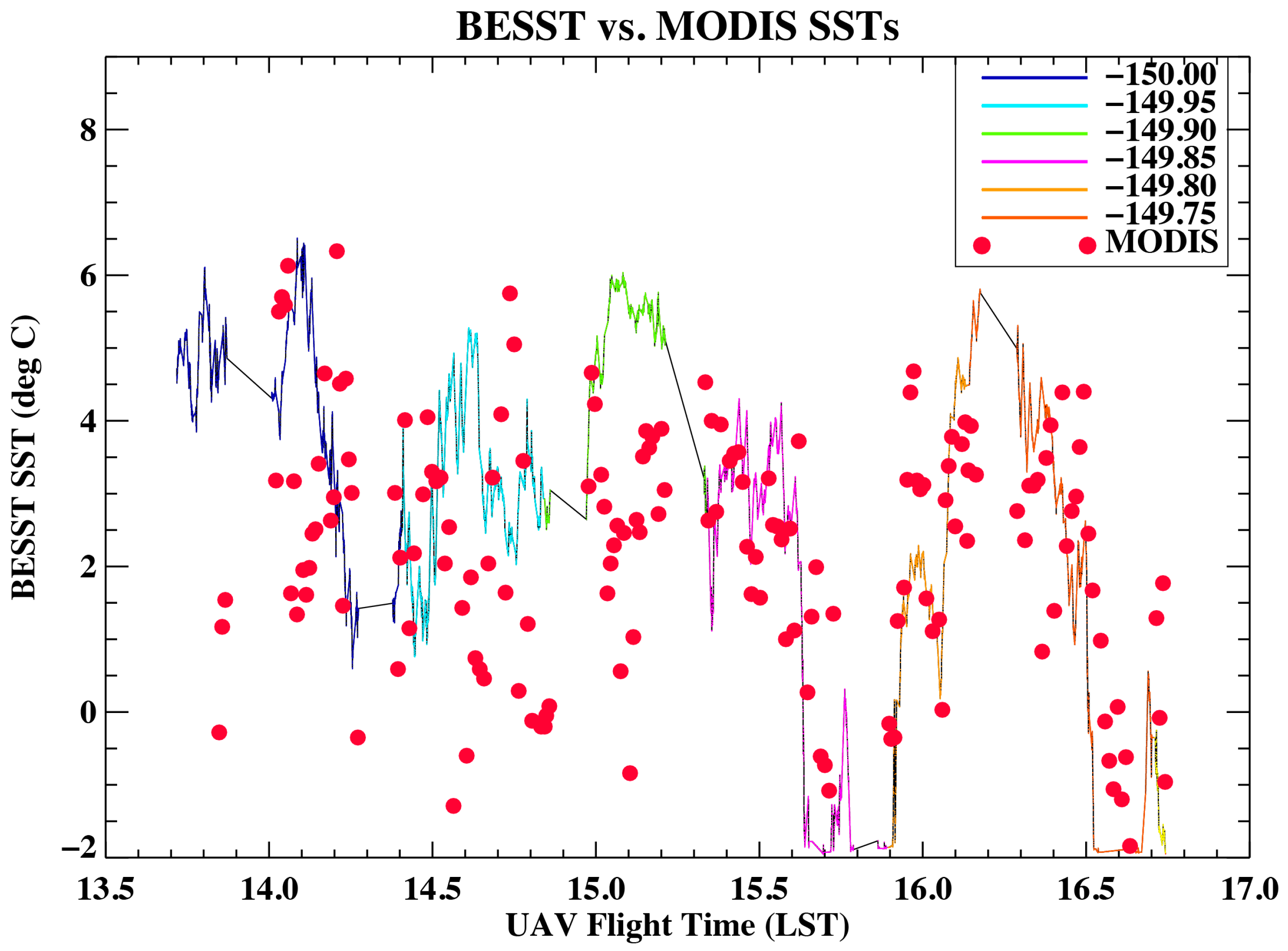
To simultaneously geolocate and collocate the BESST data, we first assigned the latitude, longitude, and time records from the Piccolo, starting from when the aircraft was still parked on the runway, to BESST, even though the latter underwent checkup procedures for about an hour prior to the Piccolo start time. The lag time between the two data records was found through trial and error by successively matching the measurements from the two radiometers, then shifting the BESST data records by a variable number of time steps and re-evaluating the matchups with MODIS until the discriminative features in both of the time series of matches overlapped when plotted together. The metric used to determine simultaneity between the time series was the correlation coefficient of the set of matches. A peak correlation of 0.43, which corresponded to a lag of 50 min, was deemed appropriate to geolocate the BESST point measurements.
The location information just derived was further used to separate the BESST data into flight segments along meridional transects. Figure 3 shows the back-shifted BESST time series of SSTs for a 50-min lag with corresponding MODIS matchups. The BESST SSTs are color coded by the predicted location of the flight tracks along meridional transects. Despite a global correlation of 0.43, it can be seen from Figure 3 that the agreement between the BESST and MODIS SSTs is good for the last three transects (correlation for the last three legs is 0.77). Correlations for the matchups along −149.85°, −149.80°, and −149.75° longitude are 0.73, 0.75, and 0.78, respectively. The good agreement between the BESST and the MODIS background temperatures for the last three transects is further exemplified in Figure 2, which also shows the geolocated BESST track, superimposed on the MODIS SST composite, color coded by BESST SSTs.
The poorer correlation between MODIS and BESST for the first three transects could have been for any number of reasons, but the BESST observations being significantly warmer than the MODIS SSTs could be an indication that the MODIS measurements over these transects were contaminated by clouds, and hence appear colder than their actual value should have been. It is important to note that the BESST values were obtained below the cloud level. Moreover, due to the scarcity of satellite data coverage during the experiment, we opted to ignore the quality assessment of the MODIS data, as suggested by the data producer. The satellite sea ice concentration (SIC) product from the National Snow and Ice Data Center (not shown) indicated that the study area had a 60% ice concentration at the time of the flight, which was desirable for the overall campaign, as this was a study of the SST conditions in the MIZ. Most SST analyses do not report SST values when the SIC is 50% or higher, which means that there is no other satellite SST product available that can be used to corroborate the cold MODIS SSTs (the more stringent cloud clearing of the VIIRS SSTs produced no matches for this place and time). For the remainder of this paper, special attention will be given to the last three transects of the flight. It should be kept in mind that the use of MODIS thus far is to give an approximate location of the BESST radiometer, so that the observations can be separated and analyzed by transects. It should not affect the BESST centric analyses, as they do not rely on the MODIS SSTs directly.
4. Data Analysis
4.1. Spatial Variability
Since the goal of this paper is to see whether the BESST measurements provide accurate information about the sub-pixel variability within 1-km footprints, we look at the BESST SST variations within the MODIS grid. The metric of choice is the standard deviation, σ, of the BESST measurements that fall within an individual MODIS pixel. The standard deviation is used to estimate sub-pixel variability, because it gives a measure of the dispersion (variation) of the SSTs along 1.25-km flight line segments, as the aircraft flies over an area the size of the MODIS pixel. This analysis could have been done independently of the satellite just by binning the entire BESST record using a bin width, or horizontal grid point spacing that encompasses the scales of interest. The reason we concentrated on the subset of BESST measurements paired with MODIS is to be able to use the satellite SSTs as reference for interpreting features in the variability gathered from the BESST. The normalized frequency distribution (or probability mass function, PMF) for the sample standard deviations of BESST SST within MODIS pixels is shown in Figure 4. The frequency distribution of σ is right-skewed, with a peak value of O(0.1) K, and a long right tail extending to a maximum of 0.8 K. The corresponding cumulative density function (CDF) shows that 95% of the pixels had σ < 0.45 K. It is interesting to note that the sub-pixel variability of this magnitude is comparable to the 0.4 K accuracy requirement for operational satellite SSTs, as cited by the Group for High Resolution Sea Surface Temperature (GHRSST) (e.g., Table 6.1 in the recommended GHRSST data specification document [19]). If the MODIS retrieval were to be validated against a point or very high spatial resolution measurement, temperature variability within the satellite pixel alone could cause differences equal to the required accuracy. The satellite minus validation difference would not accurately reflect the uncertainty in the satellite retrieval itself. In this manner, sub-pixel variability becomes a relevant component of the total uncertainty budget when satellite retrievals are validated against observations of finer resolution. The peak value of O(0.1) K in the sub-pixel variability corresponds very well to the uncertainty contribution from spatial variability found by [15] for in situ skin SSTs measured with state-of-the art IR radiometers deployed from ships.
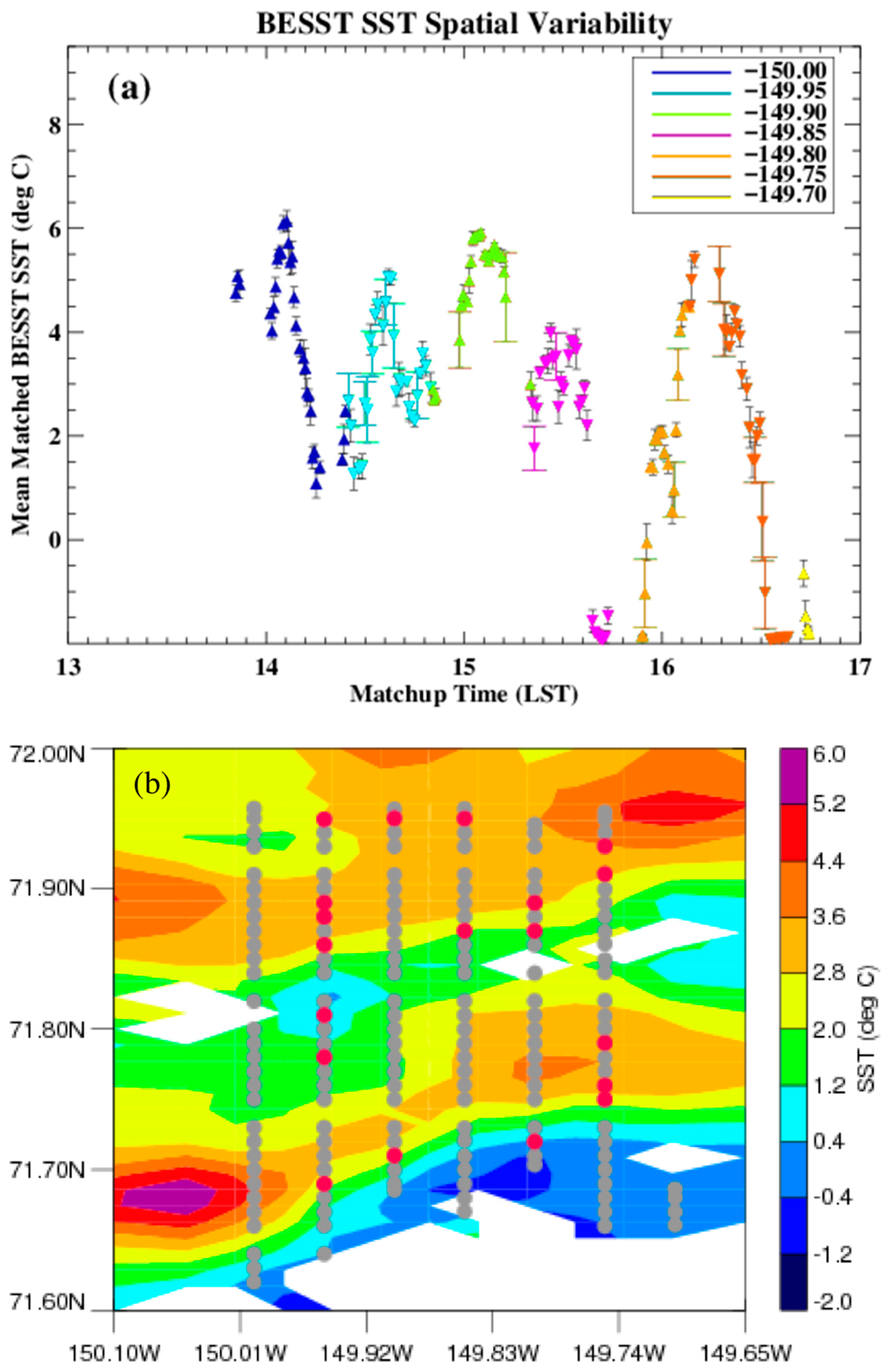
A long-tailed probability distribution can be interpreted as a statistical expression of intermittency or patchiness in the spatial and temporal distribution of submesoscale structures in the ocean surface [9]. This intermittency is manifested in the instantaneous patterns of surface temperature, density, and vorticity. Unfortunately, the 2D BESST images were reduced to linear transects of data to dampen the noise in the microbolometer, and thus, any visual indication of SST intermittency was significantly degraded. In order to look at where the high variability SST patches occurred, we looked instead at the time series of binned, MODIS-matched, BESST SSTs (Figure 5). From the collocation procedure described above, these are area-binned SSTs that result from averaging all of the BESST temperatures within 1.25-km cells, which are coincident with the MODIS grid. The triangles in Figure 5a correspond to the mean SSTs within the 1.25-km pixels of the MODIS MVC. Once again, the color of the triangles indicates the flight transect. The vertex of the triangles points to the flight direction of the UAV. Error bars correspond to 1-σ noise levels of the BESST measurements within the pixels. These error bars are a graphic representation of the spatial variability within the pixel. Colored error bars indicate grid cells where the standard deviation exceeded 0.4 K. Interestingly, the preferred location of pixels with high spatial variability was at the start and end of the meridional transects (Figure 5a).
To investigate whether the spatial distribution of high-variability pixels coincided with places of strong ocean dynamics, we looked at a contour map of the MODIS SST MVC shown in Figure 3, with the survey domain enlarged (Figure 5b). White areas are gaps in coverage due to clouds in the MODIS data. The dots show the location of the BESST matchups. Red dots indicate pixels where the standard deviation of the 1.25-km averaged BESST SSTs reflects the spatial variability in excess of the SST accuracy requirement of 0.4 K (i.e., where point-to-pixel differences can comprise a significant portion of inferred SST uncertainty estimates). The SST contour levels reveal a likely icy patch at the southern edge of the survey (water at freezing temperature), followed by alternating warm and cold filaments at mid-range and a warm area in the top third of the survey domain. There appears to be multiple surface vortices/eddies present in the warm patches of water. With the exception of the red dots at the northern end of the transects along −149.95°, −149.90°, and −149.85° longitude, which appear to be related to the aircraft turning 90 degrees, all other high-variability pixels are located at or near regions with strong temperature gradients. If, as the evidence suggests, the area of interweaving warm and cold waters corresponds to the MIZ, then the transition zones at the ice edge and at the open water edge of the MIZ are where the high variability took place. The high-variability patches at the bottom end of the survey, in particular, align extremely well with the thermal front (there is an SST change of roughly 3.5 °C over 10 km) that marks the transition between the icy patch and the warm filament. This is consistent not only with long tail statistics [9], but also with horizontal density/temperature gradients (fronts) being a primary source of submesoscale intermittency near the surface (e.g., Thomas et al. [1]; Boccaletti et al. [8]; and Samelson and Paulson [20]). To look for more statistical evidence that the asymmetric distribution of the SST sub-pixel variability in the MIZ is the result of a submesoscale transition regime that develops near horizontal temperature gradients, we did some spectral analysis of the SST, which is shown next.
4.2. Spectral Analysis of SSTs
When dealing with spatial variability, one has to deal with the concept of “scale”. In order to look at the spatial scales resolved by each of the IR radiometers, we next estimate the horizontal wavenumber spectra, for the BESST and the MODIS SSTs, using fast Fourier transforms. This methodology is appropriate to look at the scale content of oceanic variability, since the data were sampled at a regular interval. We emphasize that the spectra shown below are representative of the horizontal SST variance at the surface of the ocean (0 m depth), as both MODIS and BESST instruments have penetration depths on the order of 10–20 microns, which corresponds to the skin temperature of the ocean.
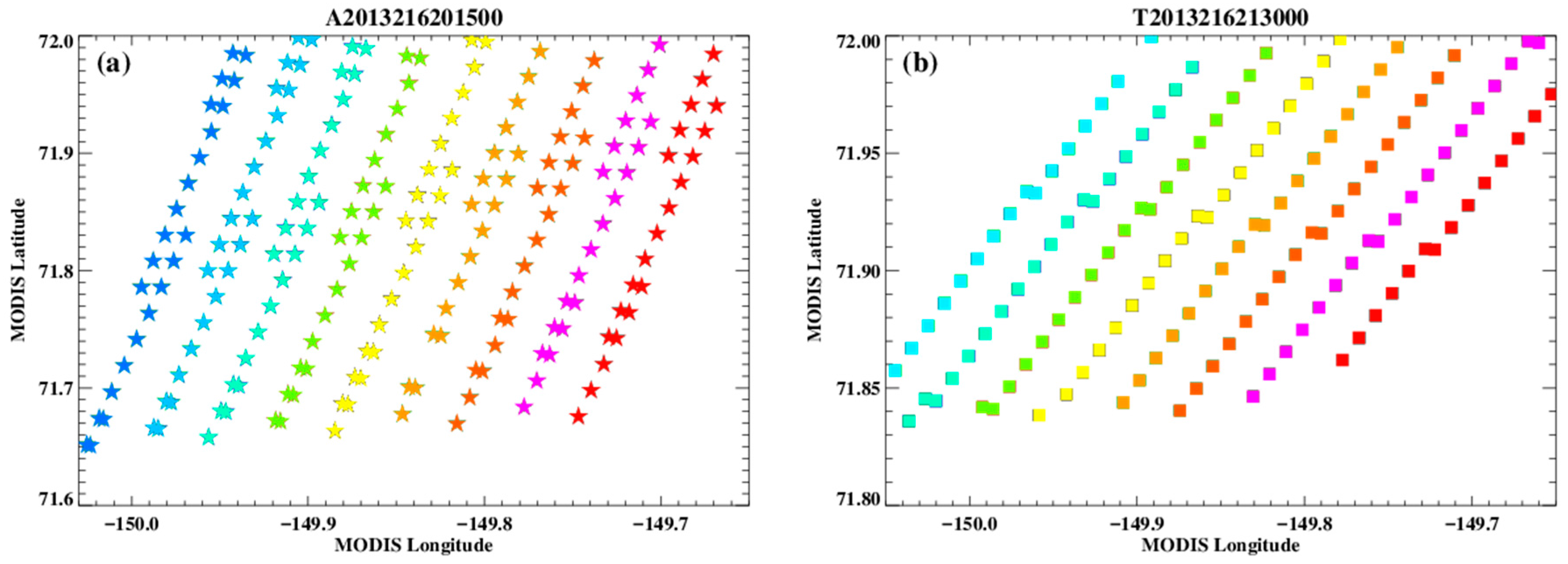
The MODIS SST horizontal wavenumber spectra were evaluated directly from the satellite swath data, as the level 2 product (geolocation is given in original satellite scan line/spot geometry) has higher spatial resolution than the MODIS maximum-value composite. Only the granules from the 20:15-Aqua and the 21:30-Terra overpasses were used in this analysis, as the other two lacked the complete data coverage and spatial continuity needed for a spectral analysis. The satellite wavenumber spectra are computed in the satellite along-track direction. Figure 6a,b show the portions of the MODIS scans over the survey area for the two granules considered. The Aqua granule covers an area approximately 250-km wide across-track by 400 km along-track, which is twice as much as the Terra granule. The dots indicate the center location of the 1-km pixels and the colors identify the selected scan spots, from successive scan lines, used to estimate the individual spectra. The sequence of successive scan spots was mostly complete over the survey domain, but in the few instances where there were gaps, these were interpolated by averaging the nearest neighbors to the selected scan spot.
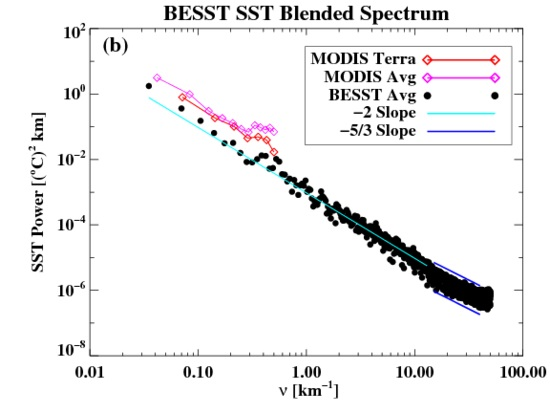
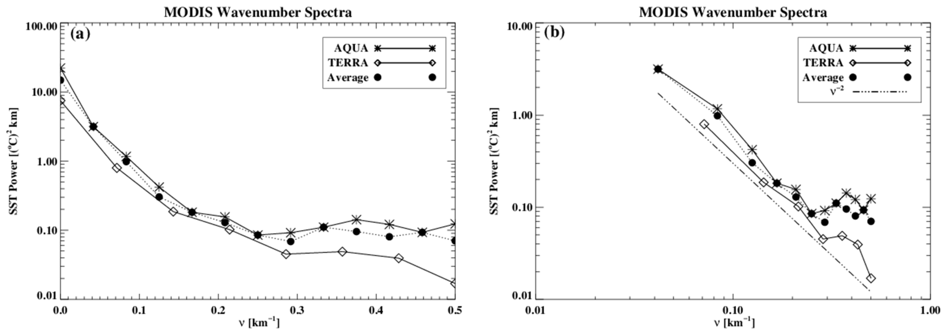
The wavenumber spectra from the individual along-track scan spots were binned to a common wavenumber, ν, scale and band-averaged to obtain a blended wavenumber spectrum representative of their collective distribution in space. The selected wavenumber bandwidth was ∆ν = 0.0417 km−1 (or 24 km) for Aqua, and ∆ν = 0.0714 km−1 (or 14 km) for Terra. By averaging over wavenumbers in these bandwidths, the spectral densities for each of the satellites are assumed to be approximately constant over the 14–24-km length-scale range. The blended spectrum is a smooth spectral density estimate that is penalized by a loss in wavenumber resolution. In other words, we cannot resolve wavelengths finer than half the corresponding wavelength (i.e., ~7–8 km). Figure 7 shows the resulting blended spectra for the Aqua and Terra granules, in km−1, in both semi-log and log–log scales. An Aqua–Terra ensemble-averaged wavenumber spectrum for MODIS is also shown in Figure 7.
The logarithm of the MODIS SST spectra against wavenumber, as displayed in Figure 7a, show very similar shapes for both the Aqua and Terra satellites, with a smooth exponential decay in power and no predominant peaks at the observed wavelengths. The log–log plot of the spectra (Figure 7b) shows that both the individual and the blended spectra are very nearly proportional to ( is horizontal wavenumber) in the range 0.04 < ν < 0.125–0.25 km−1, which corresponds to wavelengths between 25 and ~ 4–8 km. Near 4 km, the –2 power law breaks down, and a spectral peak appears close to λ = 3 km (ν = 0.33 km−1) in these three spectra, followed by a decrease toward the Nyquist wavelength (2 km). This log–log linear spectral shape with a slope of –2 is consistent with previous findings of horizontal wavenumber spectra of surface-layer temperature and density scaling as over horizontal scales of O(1)–O(100) km at mid-latitudes [20,21,22]. Thus, a slope of −2 in the temperature spectrum is consistent with submesoscale activity being the dominant source of the horizontal temperature variance, not only in the open oceans but, as our results suggest, in the MIZ as well. Since the total power (excluding the zero-term) will tend to equal the variance of the signal, the MODIS wavenumber spectra suggest that the source of the sub-pixel variability of satellite-derived SSTs within footprints of 1-km resolution resides in the submesoscale range. Dominant submesoscale features over the survey domain likely arise from temperature gradient production mechanisms such as frontogenesis and frontal instabilities.
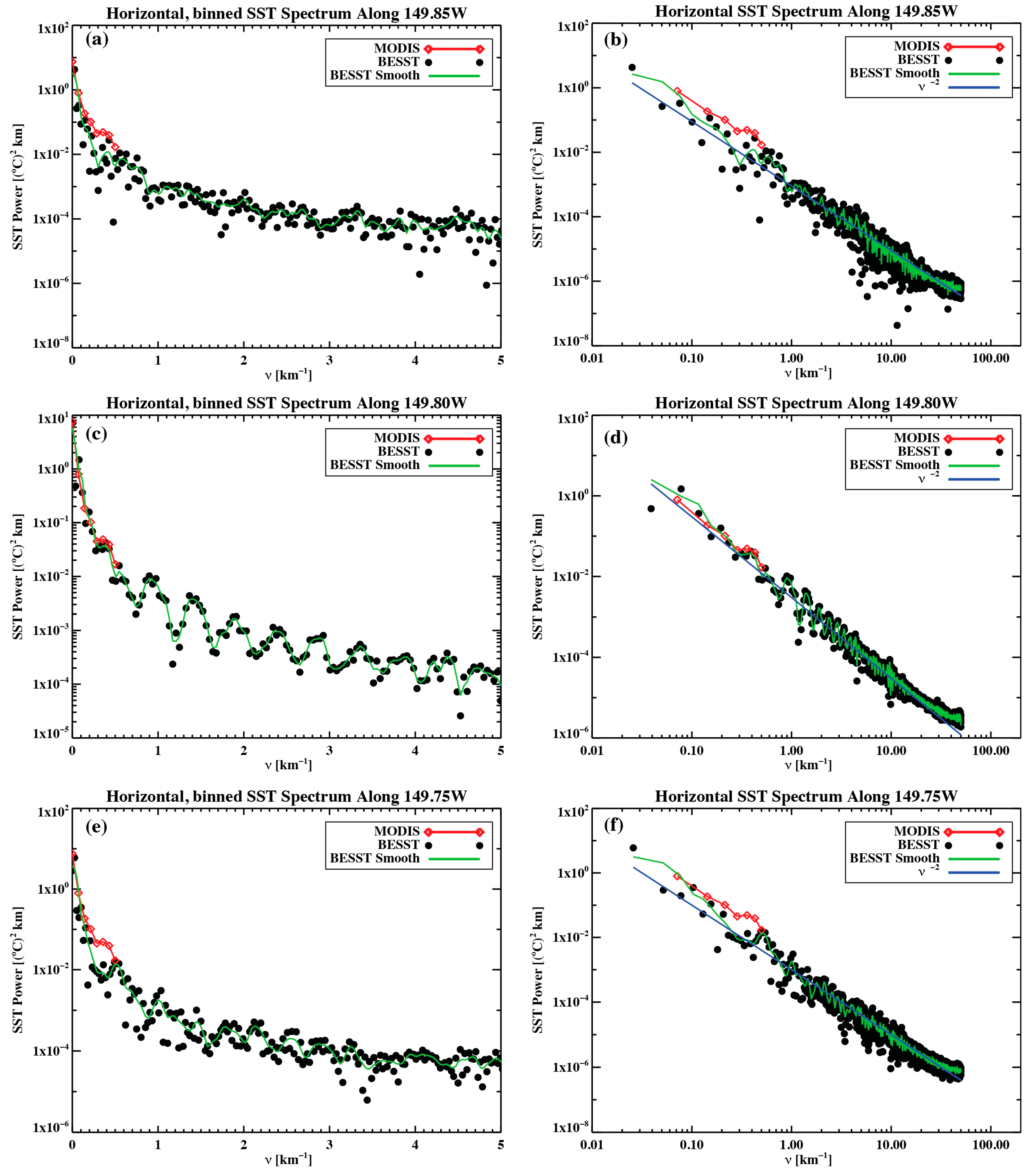
The BESST wavenumber spectra were computed along individual meridional transects, and for the entire survey. A BESST wavenumber spectrum over the lawn-mower survey is possible under the assumption that the lawn-mower sampling was on a uniform grid. However, since the BESST frame separation varied in length around 10 ± 3 m, it was necessary to interpolate the BESST data onto a uniform 10-m length meridional grid before estimating the wavenumber spectrum along individual meridional transects. This grid resolution is consistent with the mean separation of the overlapping BESST frames. Figure 8 shows the horizontal wavenumber spectra, in km−1, of the 10-m gridded BESST data along the meridional transects 149.85°W, 149.80°W, and 149.75°W, both in semi-log (left column) and log–log scales (right column), respectively. The wavenumber spectra for the transects that are not shown are very similar to those displayed in Figure 8. The collective MODIS Terra spectrum, in red, is also plotted for comparison. The black circles represent wavenumber spectra without any smoothing, whereas green traces depict spectra that were smoothed with a Tukey filter over 1-m length intervals. The density clustering of the circles illustrates clear determination of the BESST spectral shape for ν > ~2.5 km−1 (), but under determination for ν < ~1 km−1 (i.e., for scales approaching the spatial resolution of the satellite). In all cases, the log–log plots of the spectra have a shape (this is illustrated in Figure 8 by the agreement between the smoothed spectrum in green and the theoretical spectrum in dark blue) in the wavenumber range 0.04 < ν < 40 km−1 (25 km > > 0.025 km). A spectral slope of −2, once again, is a signature of submesoscale activity driving the surface temperature variability. The BESST spectrum extends the submesoscale range (10 km–100 m) at the finer wavelength resolutions an order of magnitude higher than most previously reported (from 100 m to ~25 m). A flattening of the slope occurs at ν ~40 km−1 ( ~25 m), as the scales approach what can be resolved at the BESST resolution; thus, the change in slope might just reflect noise in the BESST data or aliasing of overlapping BESST measurements.
The spectral slopes of BESST and MODIS show excellent agreement despite the BESST spectra being less resolved at the low wavenumber end where both spectra overlap. Interestingly enough, the low wavenumber end of the semi-log spectrum along 149.80°W is indistinguishable from the MODIS Terra spectrum shown in red, with both spectra showing the same shape, featuring a spectral peak at 3 km (Figure 8c). This is surprising given the different nature of the instruments. The other two spectra (Figure 8a,e) show a broad peak around 1.5 km, outside the MODIS domain. In these two cases, the spectral levels between the two vary by roughly half a decade. A key aspect of this comparison is that the BESST high-resolution SST data spans the spectral slope of −2 by ~3 decades in relative to MODIS, from 8 km to 25 m. This result, in a sense, validates the satellite findings. Since step functions also have Fourier transforms proportional to [20], the MODIS behavior could possibly be interpreted as an artifact due to the presence of sharp fronts (the spectral slope of −2 in MODIS breaks down at 8 km, whereas the MODIS composite indicates the presence of frontal widths of ~10 km). However, the behavior from BESST persisting to sufficiently small scales where fronts do not resemble step functions corroborates that the spectral behavior observed by both instruments is not an artifact due to the presence of sharp fronts (step functions). Instead, it is an artifact from the secondary circulations associated with fronts where submesoscales are found to occur. In essence, the BESST instrument expands the behavior resolved by the satellite well beyond the range of horizontal scales (by at least a decade in ) required to capture the submesoscales ( according to Kunze et al. [23]).
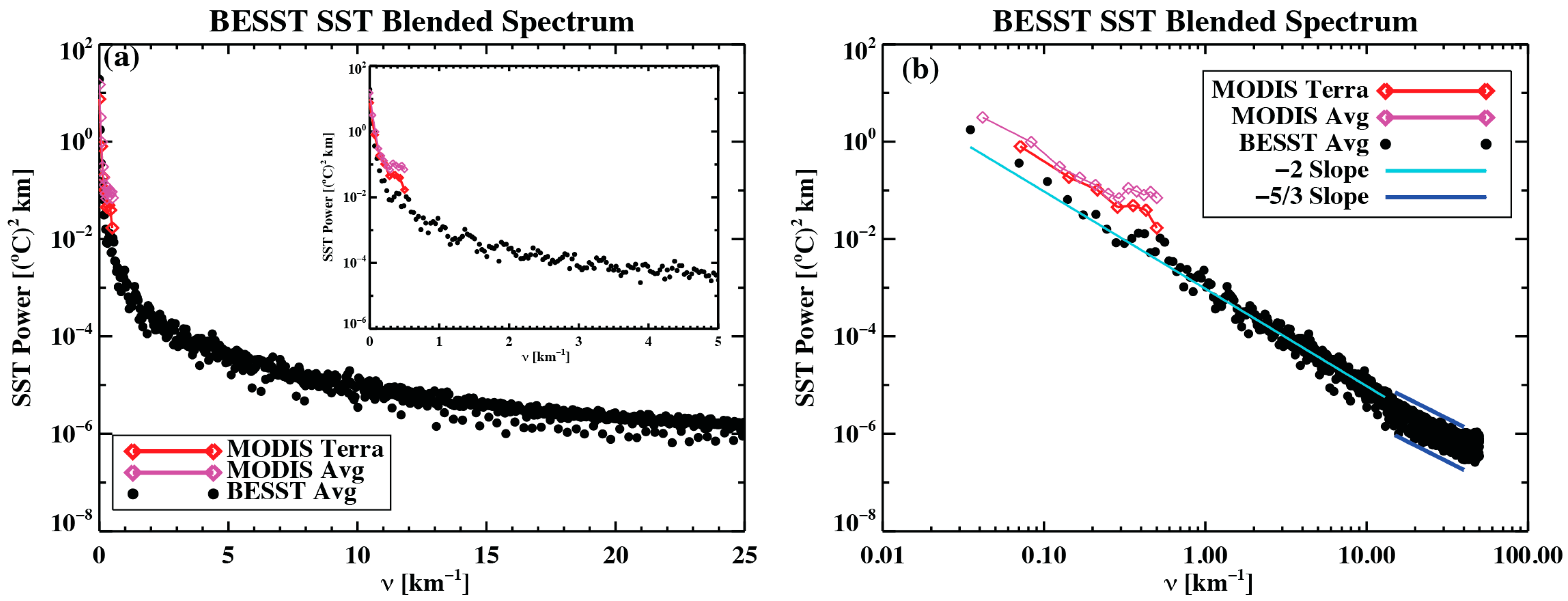
For a blended BESST horizontal wavenumber spectrum representative of the whole survey area, the wavenumber spectra from the individual meridional transects were binned into non-overlapping, sequential wavenumber bands of width Δν = 0.0286 km−1 (or equivalently, Δλ = 35 km). In a manner consistent with the procedure used to derive the MODIS blended spectra, the ensemble-averaged BESST wavenumber spectrum for the survey domain was defined as the bin-wise average of the Fourier coefficients from the spectra from the six individual, uniformly gridded, lawn-mower transects. The ensemble waveband-average BESST wavenumber spectrum representative of the spatial domain is shown in Figure 9. The spectral distribution shown here is qualitatively very similar to the ones in Figure 8 for the individual transects, although they are also smoother due to the loss of wavenumber resolution resulting from the binning process. However, the low wavenumber end of the spectrum is better resolved, as it shows an offset of less than 0.5 decades in spectral power with respect to the MODIS spectra in the overlapping range. The log–log spectrum (black dots) in Figure 9b has a shape of in the wavenumber range 0.04 < ν < 10 km−1 (100 m–25 km horizontal wavelengths), spanning from the small to the submesoscales, as shown by the agreement with the light blue line representing a −2 spectral slope. The shape of the spectrum confirms, once again, that a substantial portion of the variance in the SST field over the 0.04- to 10-km−1 band is likely due to submesoscale processes present in the region at the time of the survey. The small peak present in the MODIS spectra at λ = 3 km is well resolved in the blended BESST spectrum, but appears shifted towards a slightly higher wavenumber (λ = ~2 km).
An interesting remark is that the break in the −2 slope for the blended spectrum happens at a longer wavelength than in the individual BESST spectra (100 m vs. 25 m). The bend in the spectrum observed here at λ = ~100 m is consistent with a transitioning regime from the submesoscale to small-scale flows. While the occurrence of this transition cannot be ascertained from the individual spectra in Figure 8, as the bend occurs near scales where the noise becomes predominant, noise has been significantly dampened in the blended spectrum, which is shown in Figure 9. Furthermore, the semi-log spectrum (Figure 9a) also shows a notable decrease in the spread of spectral power with wavenumber for ν > ~10–13 km−1 (~80–100 km). The relevant aspect is that the spectral slope changes from −2 to −5/3, as shown by the dark blue lines bracketing the second regime in Figure 9b. The scaling persists from ~10 < ν < 40 km−1 (~100 m > > 25 m). A slope of –5/3 is consistent with the Kolmogorov spectrum for microscale turbulence [24]. Using Kolmogorov-like dimensional analyses, Obukhov [25] and Corrsin [26] predicted a temperature spectrum with a slope of −5/3 at the small-scale inertial range. Wavenumber spectra with two separate power law scalings have been reported [27,28]. If this is indeed the case, the horizontal SST variance transitions from a regime driven by submesoscale dynamics to an inertial regime driven by microscale turbulence at horizontal scales on the order of meters. However, conclusive evidence of a meaningful transition and a spectrum with dual power law scaling requires more in depth study.
5. Conclusions
The aim of this paper was to evaluate if, by flying an IR radiometer on a fast-moving platform such as an UAV, it would be possible to resolve the horizontal scales of SST variability in the MIZ. Moreover, we attempted to quantify how this spatial variability could impact uncertainty estimates of satellite-derived SSTs within 1-km footprints when validated with observations on finer spatial scales. The measurement campaign took place during a period of highly dynamic processes at the start of the melt season in the southern Beaufort Sea. Wavenumber spectral analyses from MODIS and the UAV-deployed BESST radiometer were used to describe horizontal SST variance over lengths of 0.025–25 km. Wavenumber spectra for both MODIS and BESST systematically showed a uniform spectral slope of −2 (Figure 7, Figure 8 and Figure 9) for wavenumbers in the range 0.04 < ν < 40–50 km−1 (25 km > > 25–100 m). The BESST blended spectrum for the region also suggests a second power law with −5/3 slope for λ < 100 m, which is consistent with the Kolmogorov–Obukhov–Corrsin power law scaling for the SST energy spectrum in the microscale turbulence regime. However, this requires further verification. The slopes of the BESST spectra not only aligned naturally with the satellite spectra at low wavenumbers, but also extended its range of horizontal wavenumbers (length scales) to higher ν (smaller ), by about three orders of magnitude. A spectral shape of is consistent with the submesoscale processes at the surface. So, it appears that the submesoscale features project onto a wide wavenumber spectrum, as seen when taken both individually and through their collective distribution in space [29]. Our interpretation is that the submesoscale processes increase the variance of the spatial distribution of tracers at the ocean surface, and hence are responsible for the horizontal scales contributing to the SST sub-pixel variability in the MIZ and in the open ocean. This is also supported by the long-tail probability distribution of the sub-pixel SST variance from BESST, which indicates strong patchiness (spatial variability) within 1-km footprints. Moreover, MODIS pixels with high spatial variability appeared to be associated with thermal fronts, where submesoscales are prone to occur. It is important to emphasize that the BESST observations were collected below cloud base, so cloud effects should not impact the observed variability.
Knowledge of the spectral slope alone is not sufficient to draw conclusions about the physical processes responsible for the observed SST variance in the MIZ, and certainly there is not sufficient data in this experiment to prove it unequivocally. However, given the pervasiveness of the -dependence of the surface temperature variance on wavenumber for the submesoscale range, which is corroborated by extensive experimental evidence from throughout the open oceans [7,8,9,20,21,22], we speculate, with a certain degree of confidence, that submesoscale processes such as frontogenesis and submesoscale instabilities are responsible for the observed SST variability in the MIZ. This is somewhat expected if, as Saffman [29] pointed out, the energy spectrum density for random solutions of the equation:
should vary asymptotically similar to in the range of wavenumbers between the macroscale and the microscale viscous cut-off. This was proven numerically by Hosokawa [30]. The differential equation above is the Burgers solution to the modified Navier–Stokes (NS) equation, , (also known as the Hopf equation [31]), which has an additional “fluctuation” term, f, which describes a random force that incorporates the “thermal agitation” caused by molecular motion. The thermal agitation term is usually neglected from NS, in part due to computational limitations in finding an analytical solution for the random force field [30]. What this suggests is that, by considering the natural thermal agitation (e.g., temperature variability) when describing turbulent motions in the range of scales that bridge the macro with the micros (e.g., the submesoscale regime), the energy spectrum of the fluid motion scales as .
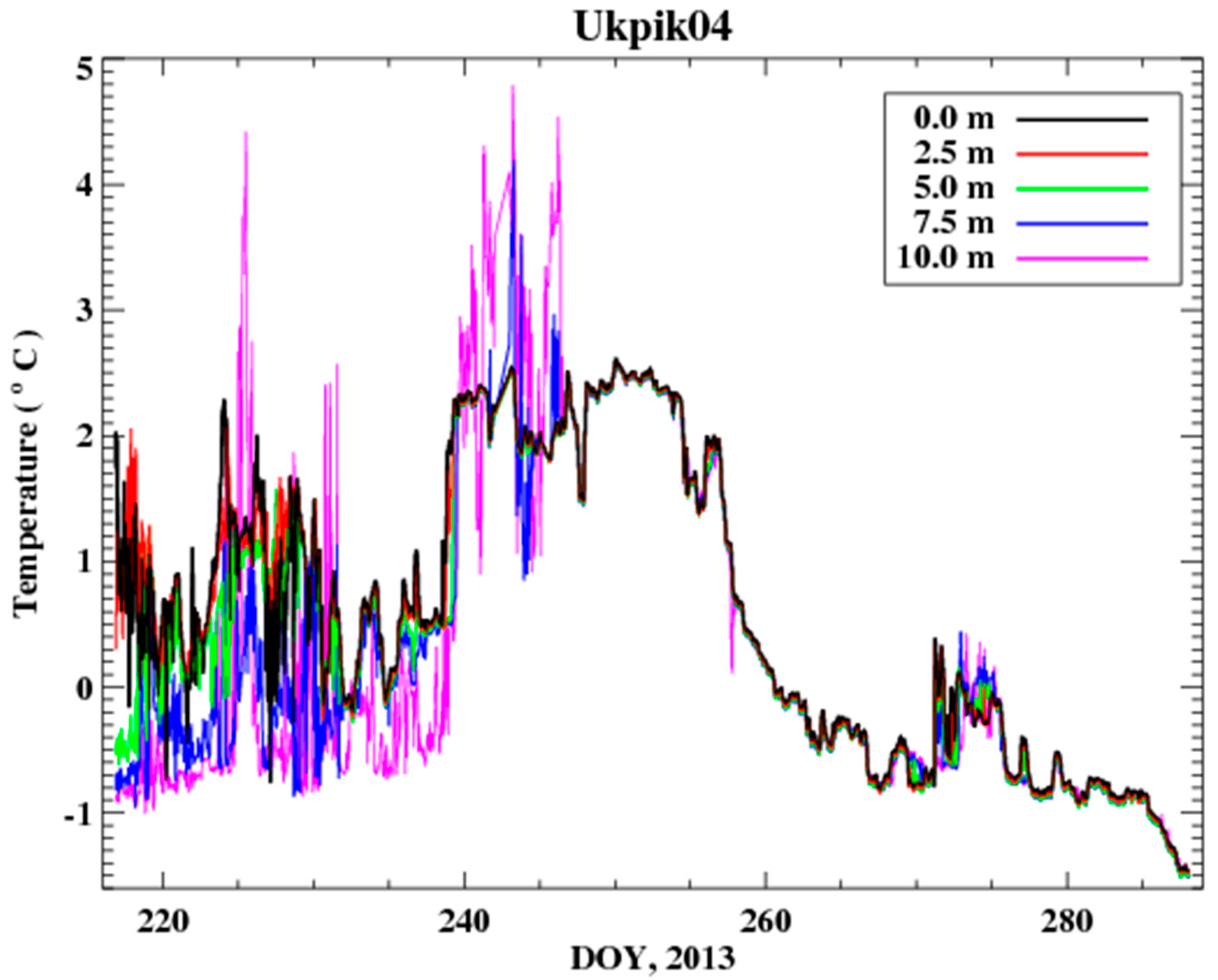
Submesoscales have temporal scales of hours to days (a couple of weeks at most). Therefore, the submesoscale variability is transient, and requires a continuous supply of variance to maintain it [23]. The examination of time series of temperatures with depth (Figure 10) from an UpTempO buoy [32], which was deployed in a nearby area (see Figure 1) as part of MIZOPEX on the same day of the survey, indicates that intense variability was present in the top 10 m of the ocean surface at the time of the UAV deployment, and persisted for 15 days after the survey. During this time, the temperature measurements from the buoy showed strong stratification in the top 10 m of the MIZ, and even a couple episodes of diurnal warming (DOY 219 and 228) in the top 2.5–5 m. After 19 August (DOY 231) 2013, the transient stratification was eradicated, and the surface layer became vertically homogenized. As shown in Figure 10, a well-mixed layer (isothermal temperature with depth) became apparent in the top 7.5 m after DOY 231, and in the top 10 m after DOY 248, which then persisted for the rest of the summer season. Similar Arctic mixed layer depths of 10–15 m were observed by Castro et al. [33] from other UpTempO buoys in the area for the summers of 2012 and 2013. Toole et al. [16] observed mixed layer depths in the Canada Basin varying between 10 and ~30–40 m over a few days during the winter; in the summer, the mixed layer depth averaged 16 m. Timmermans et al. [4] showed that mixed layers of this type are a common occurrence in the Arctic winter, and are the result of submesoscale restratification by horizontal density gradients. This circumstantial evidence, together with the spectral analyses described here, is further indicative of the importance of the submesoscales to the transient stratification that generates vertical gradients within the surface layer when atmospheric forcing is not strong enough to produce vertical mixing [4,5].
Boccaletti et al. [8] suggested that the horizontal density gradients at scales of O(1) km that restratify the surface mixed layer on temporal scales of days are the result of baroclinic instabilities at frontal regions. These baroclinic instabilities have preferred length scales of ~O(5) km. The spatial distribution of the BESST SST variance indicates that most of the sub-pixel variability is less than 0.1 K, but 5% of data can have a standard deviation well in excess of the accuracy requirements of satellite SSTs (σ ≥ 0.4 K). An SST gradient spectrum with a slope of −2 is consistent with a front no wider than the smallest resolved length scales; in our case, this means that O(5–10) km. Not only are thermal fronts of this magnitude evident in the MODIS SST composite (Figure 5), but areas of high variability measured by BESST have preferential locations at or near these fronts.
It is noteworthy that MIZOPEX was not designed as a submesoscale measurement campaign, but rather as a marginal sea ice experiment. As such, there were no complementary measurements of density, winds, and surface fluxes to help us interpret the observed variability. Field campaigns aiming to resolve the submesoscale usually have multiple autonomous instruments with nested sampling covering entire areas and providing dozens of independent realizations of the submesoscale from different tracers. It was fortuitous that the BESST measurements captured the submesoscale. By using a UAV-deployed radiometer such as the BESST system, we have somewhat unintentionally revealed new features of the wavenumber spectrum of the SST variability between the mesoscale and the small scales that can be relevant for interpreting submesoscale processes of the upper ocean as well as for understanding the spatio-temporal variability of satellite remote sensing variables in general. Moreover, the horizontal scales involved in the restratification of the Arctic Ocean surface layer are not typically resolved in numerical models, which points to the need for additional high spatial and temporal resolution data that help demonstrate the role of submesoscale lateral processes in regulating the sub-pixel variability within high-resolution satellite data.
The growing literature on submesocale processes, as cited above, suggests that their impact is ubiquitous throughout the oceans. Additional high spatial resolution data from satellites, aircraft, and other new observing technologies will help to further verify this and study the processes in detail. New generation IR satellite sensors with spatial resolutions finer than 1 km will reveal increasing levels of pixel-to-pixel variability, and submesoscale processes represent an important potential contribution to that variability. More dedicated airborne and UAV observations such as those described here will be highly beneficial in quantifying the role and nature of these processes.
Acknowledgments
Sandra Castro, William Emery, and William Tandy Jr. were supported by the MIZOPEX project through NASA award NNX11AN57G. Gary Wick and Sandra Castro were also supported in part by a grant from the NASA Physical Oceanography Program, award NNH13AV34I (Eric Lindstrom). The authors also wish to thank James Maslanik for leading MIZOPEX, William Good for his additional advice on the function and performance of the BESST, and Mathew Tooth for early analysis of the BESST data. The UpTempO buoy SSTs from the Polar Science Center at the Applied Physics Laboratory in the University of Washington were obtained from the UpTempO Buoy Project web site at http://psc.apl.washington.edu/UpTempO/. Special thanks to NASA Cryospheric Sciences Program Manager Thomas Wagner. The authors also appreciate very constructive comments provided in a review by Peter Cornillon.
Author Contributions
Sandra Castro performed the data analysis and wrote the paper; William Emery deployed the BESST radiometer and had a vision for the application of the data; Gary Wick provided suggestions on the analysis and helped edit the paper; and William Tandy contributed instrument support and insight.
Conflicts of Interest
The authors declare no conflict of interest.
References
- Thomas, L.N.; Tandon, A.; Mahadevan, A. Submesoscale Processes and Dynamics. In Ocean Modeling in an Eddying Regime; American Geophysical Union: Washington, DC, USA, 2008; pp. 17–23. [Google Scholar]
- Shay, L.; Cook, T.; An, P. Submesoscale coastal ocean flows detected by very high frequency radar and autonomous underwater vehicles. J. Atmos. Ocean. Technol. 2003, 20, 1583–1599. [Google Scholar] [CrossRef]
- Capet, X.; McWilliams, J.C.; Molemaker, M.; Shchepetkin, A. Mesoscale to submesoscale transition in the California Current system. Part II: Frontal processes. J. Phys. Oceanogr. 2008, 38, 44–63. [Google Scholar] [CrossRef]
- Timmermans, M.-L.; Cole, S.; Toole, J. Horizontal density structure and restratification of the Arctic Ocean surface layer. J. Phys. Oceanogr. 2012, 42, 659–668. [Google Scholar] [CrossRef]
- Hosegood, P.; Gregg, M.C.; Alford, M.H. Sub-mesoscale lateral density structure in the oceanic surface mixed layer. Geophys. Res. Lett. 2006, 33, 126–136. [Google Scholar] [CrossRef]
- Lee, C.; D’Asaro, E.; Harcourt, R. Mixed Layer Restratification: Early Results from the AESOP Program. 2006. Available online: http://adsabs.harvard.edu/abs/2006AGUFMOS51E..04L (accessed on 6 September 2017).
- Fox-Kemper, B.; Ferrari, R.; Hallberg, R. Parameterization of mixed layer eddies. Part I: Theory and diagnosis. J. Phys. Oceanogr. 2008, 38, 1145–1165. [Google Scholar] [CrossRef]
- Boccaletti, G.; Ferrari, R.; Fox-Kemper, B. Mixed layer instabilities and restratification. J. Phys. Oceanogr. 2007, 37, 2228–2250. [Google Scholar] [CrossRef]
- Capet, X.; McWilliams, J.C.; Molemaker, M.; Shchepetkin, A. Mesoscale to submesoscale transition in the California Current system. Part I: Flow structure, eddy flux, and observational tests. J. Phys. Oceanogr. 2008, 38, 29–43. [Google Scholar] [CrossRef]
- Mahadevan, A.; Campbell, J. Biogeochemical patchiness at the sea surface. Geophys. Res. Lett. 2002, 29. [Google Scholar] [CrossRef]
- Abraham, E. The generation of plankton patchiness by turbulent stirring. Nature 1998, 391, 577–580. [Google Scholar] [CrossRef]
- Cornillon, P.; Castro, S.; Gentemann, C.; Jessup, A.; Kaplan, A.; Lindstrom, E.; Maturi, E. SST Error Budget—White Paper. 2010. Available online: http://works.bepress.com/peter-cornillon/1/ (accessed on 6 September 2017).
- Castro, S.L.; Wick, G.A.; Minnett, P.J.; Jessup, A.T.; Emery, W.J. The impact of measurement uncertainty and spatial variability in the accuracy of skin and subsurface regression-based sea surface temperature algorithms. Remote Sens. Environ. 2010, 114, 2666–2678. [Google Scholar] [CrossRef]
- Ohring, G.; Wielicki, B.; Spencer, R.; Emery, B.; Datla, R. Satellite instrument calibration for measuring global climate change: Report of a workshop. Bull. Am. Meteorol. Sci. USA 2005, 86, 1303–1313. [Google Scholar] [CrossRef]
- Brink, K.H.; Cowles, T.J. The Coastal Transition Zone program. J. Geophys. Res. 1991, 96, 14637–14647. [Google Scholar] [CrossRef]
- Toole, J.M.; Timmermans, M.L.; Perovich, D.K.; Krishfield, R.A.; Proshutinsky, A.; Richter-Menge, J.A. Influences of the ocean surface mixed layer and thermohaline stratification on Arctic sea ice in the central Canada basin. J. Geophys. Res. 2010, 115, C10018. [Google Scholar] [CrossRef]
- Emery, W.J.; Good, W.S.; Tandy, W., Jr.; Izaguirre, M.A.; Minnett, P.J. A microbolometer airborne calibrated infrared radiometer: The Ball Experimental Sea Surface Temperature (BESST) radiometer. IEEE Trans. Geosci. Remote Sens. 2014, 52, 7775–7781. [Google Scholar] [CrossRef]
- Good, W.; Warden, R.; Kaptchen, P.F.; Emery, W.J.; Giacomini, A. Absolute Airborne Thermal SST Measurements and Satellite Data Analysis from the Deepwater Horizon Oil Spill. In Monitoring and Modeling the Deepwater Horizon Oil Spill: A Record-Breaking Enterprise; Liu, Y., Macfadyen, A., Ji, Z.-G., Weisberg, R.H., Eds.; American Geophysical Union: Washington, DC, USA, 2011; pp. 51–61. [Google Scholar]
- GHRSST Science Team. The Recommended GHRSST Data Specification (GDS) 2.0, Document Revision 5. Available from the GHRSST International Project Office (document reference GDS2.0r5.doc). 2012, p. 123. Available online: https://www.ghrsst.org/wp-content/uploads/2016/10/GDS20r5.pdf (accessed on 12 September 2017).
- Samelson, R.M.; Paulson, C.A. Towed thermistor chain observations of fronts in the subtropical North Pacific. J. Geophys. Res. 1988, 93, 2237–2246. [Google Scholar] [CrossRef]
- Cole, S.T.; Rudnick, D.L.; Colosi, J.A. Seasonal evolution of upper-ocean horizontal structure and the remnant mixed layer. J. Geophys. Res. 2010, 115, C04012. [Google Scholar] [CrossRef]
- Hodges, B.A.; Rudnick, D.L. Horizontal variability in chlorophyll fluorescence and potential temperature. Deep-Sea Res. I 2006, 53, 1460–1482. [Google Scholar] [CrossRef]
- Kunze, E.; Klymak, J.M.; Lien, R.C.; Ferrari, R.; Lee, C.M.; Sundermeyer, M.A.; Goodman, L. Submesoscale Water-Mass Spectra in the Sargasso Sea. J. Phys. Oceanogr. 2015, 45, 1325–1338. [Google Scholar] [CrossRef]
- Pope, S.B. Turbulent Flows; Cambridge University Press: Cambridge, UK, 2000; p. 771. [Google Scholar]
- Obukhov, A.M. The structure of the temperature field in a turbulent flow. Izv. Akad. Nauk. SSSR Ser. Geogr. Geofiz. 1949, 13, 58–69. [Google Scholar]
- Corrsin, S. On the spectrum of isotropic temperature fluctuations in isotropic turbulence. J. Appl. Phys. 1951, 22, 469–473. [Google Scholar] [CrossRef]
- Nastrom, G.D.; Gage, K.S. A climatology of atmospheric wavenumber spectra of wind and temperature observed by commercial aircraft. J. Atmos. Sci. 1985, 42, 950–960. [Google Scholar] [CrossRef]
- McCaffrey, K.; Fox-Kemper, B.; Forget, G. Estimates of Ocean Macroturbulence: Structure Function and Spectral Slope from Argo Profiling Floats. J. Phys. Oceanogr. 2015, 45, 1773–1793. [Google Scholar] [CrossRef]
- Saffman, P.G. On the Spectrum and Decay on Random Two-Dimensional Vorticity Distributions at Large Reynolds Numbers. Stud. Appl. Math. 1971, 50, 377–383. [Google Scholar] [CrossRef]
- Hosokawa, I. Ensemble mechanics for the random-forced Navier-Stokes flow. J. Stat. Phys. 1976, 15, 87–104. [Google Scholar] [CrossRef]
- Hopf, E. The partial differential equation ut + uux = uxx. Commun. Pure Appl. Math. 1950, 3, 201–230. [Google Scholar] [CrossRef]
- Steele, M.; Rigor, I.; Ermold, W.; Ortmerer, M. UpTempO Buoys Deployed in 2013. NSF Arctic Data Center, 2015. Available online: http://psc.apl.washington.edu/UpTempO/Data.php (accessed on 14 September 2017).
- Castro, S.L.; Wick, G.A.; Steele, M. Validation of satellite sea surface temperature analyses in the Beaufort Sea using UpTempO buoys. Remote Sens. Environ. 2016, 187, 458–475. [Google Scholar] [CrossRef]
Figure 1.
Ball Experimental Sea Surface Temperature (BESST) lawn mower survey during the Marginal Ice Zone Observations and Processes Experiment (MIZOPEX) (black). The aircraft entered the pattern heading northbound at the western edge of the pattern, and exited to the south at the eastern edge. The background image is from the Moderate Resolution Imaging Spectroradiometer (MODIS) AQUA sea surface temperature (SST) granule for 20:15 UTC on 4 August 2013, the day of the flight. The blue trace depicts the UpTempO buoy track while in the study area. This buoy was deployed the day after the unmanned aerial vehicle (UAV) survey, and was part of the MIZOPEX in situ instruments.
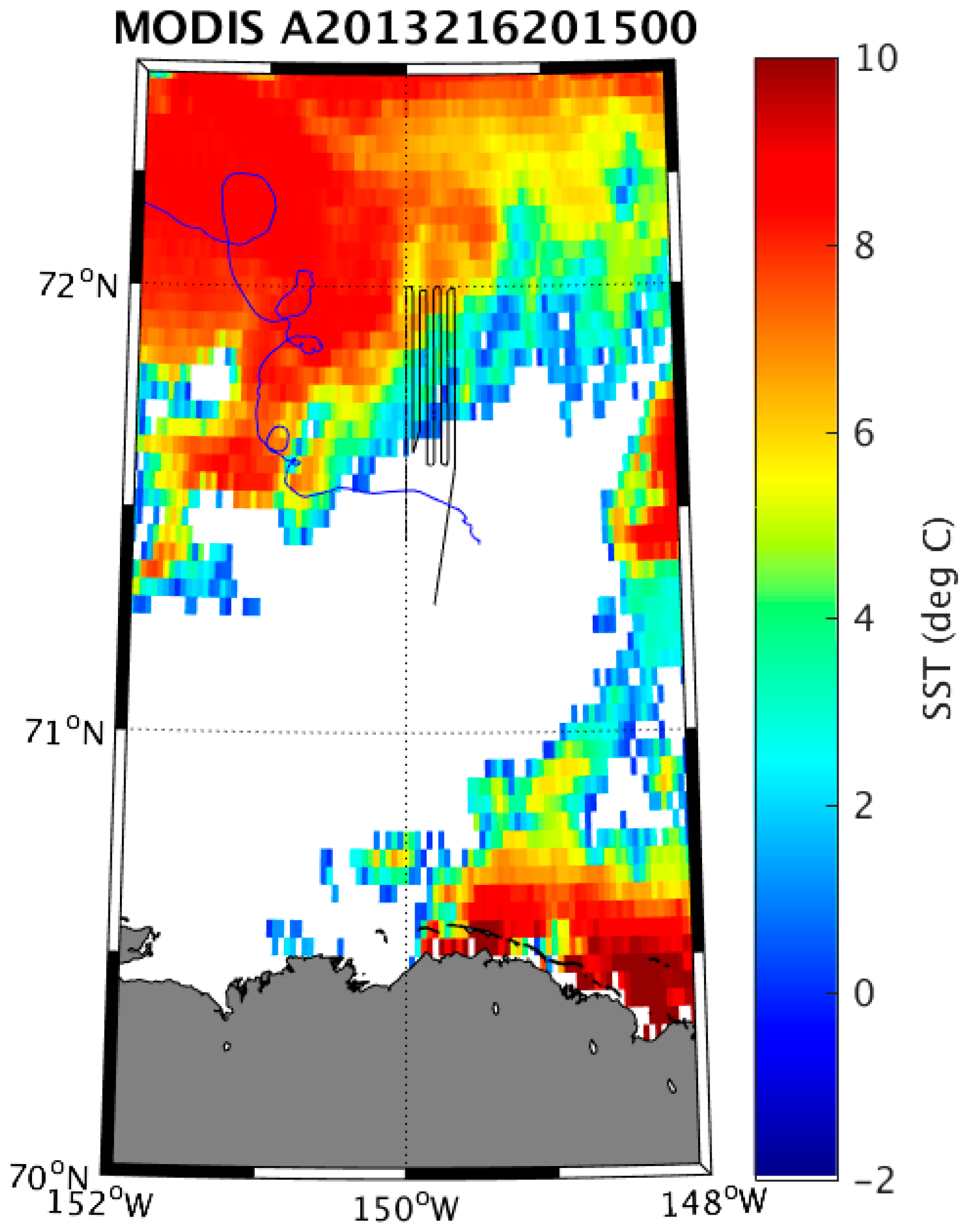
Figure 2.
MODIS SST Maximum Value Composite with superimposed BESST back-shifted tracks, color-coded by the corresponding BESST SSTs. The western track was sampled first, with the aircraft heading northbound.
Figure 2.
MODIS SST Maximum Value Composite with superimposed BESST back-shifted tracks, color-coded by the corresponding BESST SSTs. The western track was sampled first, with the aircraft heading northbound.
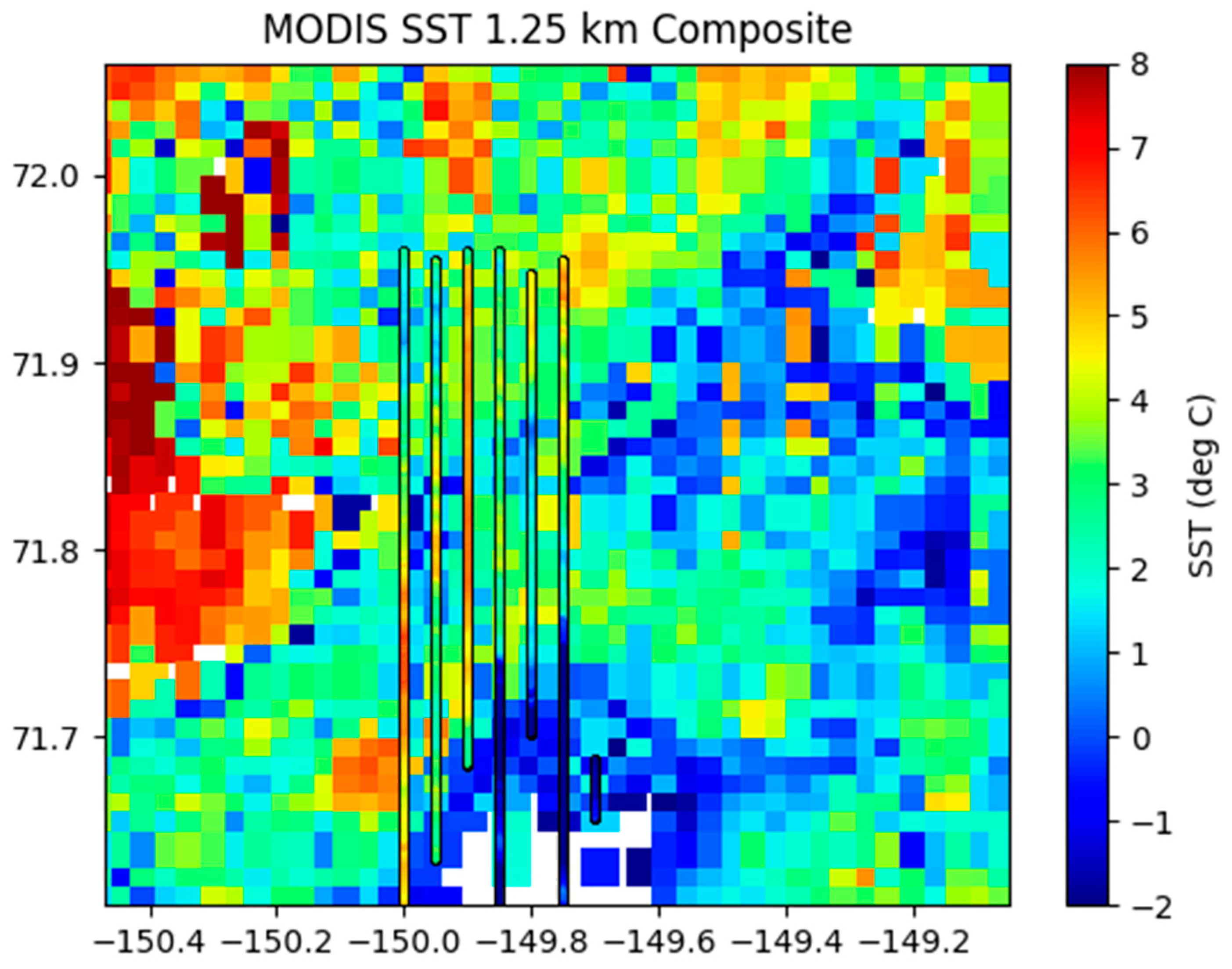
Figure 3.
BESST SST time series, shifted back in time by 50 min, with superimposed MODIS SST matchups (red dots) from the maximum value composite.
Figure 3.
BESST SST time series, shifted back in time by 50 min, with superimposed MODIS SST matchups (red dots) from the maximum value composite.

Figure 4.
Probability mass function (a) and cumulative density function (CDF, (b) for the standard deviations of the BESST measurements within the MODIS Maximum Value Composite (MVC) SST pixels.
Figure 4.
Probability mass function (a) and cumulative density function (CDF, (b) for the standard deviations of the BESST measurements within the MODIS Maximum Value Composite (MVC) SST pixels.
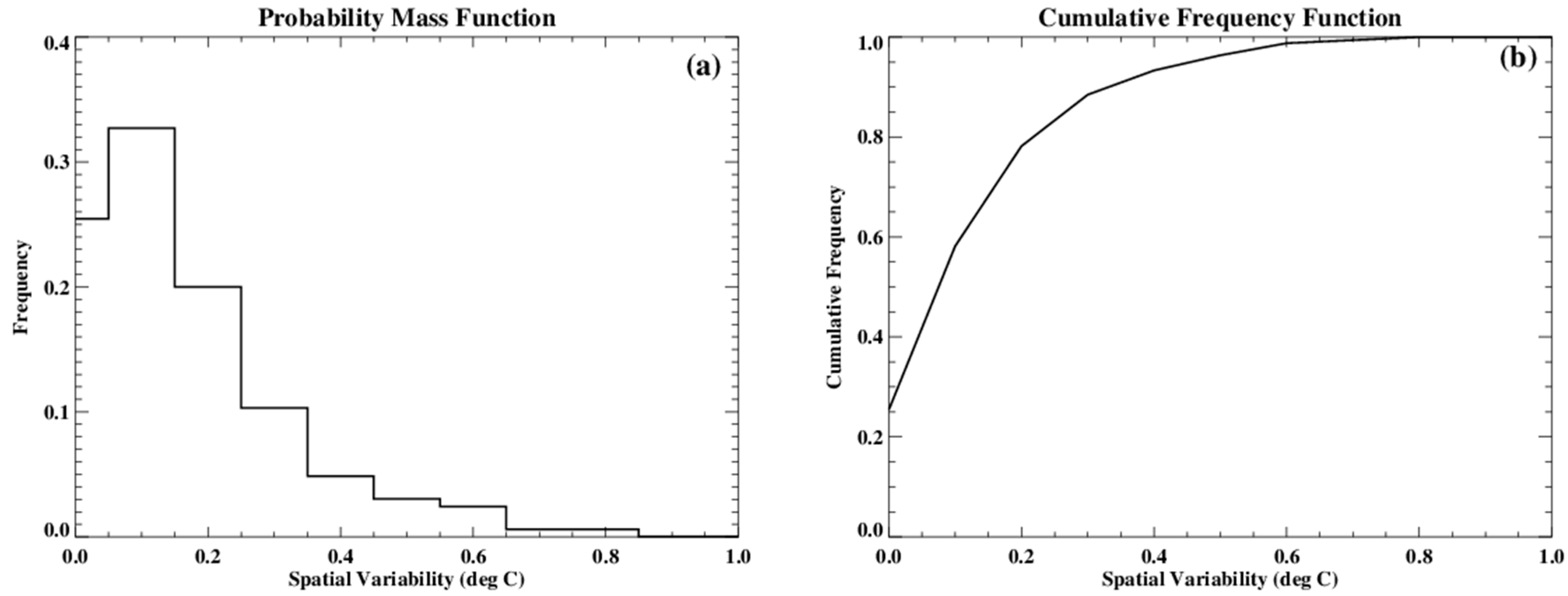
Figure 5.
Time series (a) of time-lagged BESST SSTs matched to MODIS. The triangles represent the mean BESST temperature within the MODIS pixel. The color and vertex of the triangle indicates the flight transect and direction, respectively. Error bars correspond to 1-σ variability. Where σ ≥ 0.4 °C, the error bar is color coded by transect. The SST map shown in (b) is a contour representation of the MODIS composite (Figure 2) around the BESST survey (grey circles). Red circles illustrate the location of the BESST area-averaged measurements with σ ≥ 0.4.

Figure 6.
MODIS along-track scan spots for the Aqua (a) and Terra (b) granules that were used to compute the satellite horizontal wavenumber spectra.
Figure 6.
MODIS along-track scan spots for the Aqua (a) and Terra (b) granules that were used to compute the satellite horizontal wavenumber spectra.

Figure 7.
Ensemble-averaged, band-average horizontal wavenumber spectra for SST variance from MODIS, along the (a) semi-log and (b) log–log axes. MODIS spectra are very nearly proportional to the theoretical spectrum
Figure 7.
Ensemble-averaged, band-average horizontal wavenumber spectra for SST variance from MODIS, along the (a) semi-log and (b) log–log axes. MODIS spectra are very nearly proportional to the theoretical spectrum

Figure 8.
(a–f) Horizontal wavenumber spectra for SST variance from BESST, along the semi-log (left) and log–log axis (right), and along meridional transects: 149.85°W, 149.80°W, and 149.75°W.
Figure 8.
(a–f) Horizontal wavenumber spectra for SST variance from BESST, along the semi-log (left) and log–log axis (right), and along meridional transects: 149.85°W, 149.80°W, and 149.75°W.

Figure 9.
Blended BESST wavenumber spectrum over the entire survey domain. (a) Semi-log spectrum with the inset highlighting the range from 0–5 km−1; (b) Corresponding log–log spectrum along with overlays of spectral slopes of −2 and −5/3 in the light and dark blue colors, respectively.
Figure 9.
Blended BESST wavenumber spectrum over the entire survey domain. (a) Semi-log spectrum with the inset highlighting the range from 0–5 km−1; (b) Corresponding log–log spectrum along with overlays of spectral slopes of −2 and −5/3 in the light and dark blue colors, respectively.

Figure 10.
Temperatures in the top 10 m from the MIZOPEX UpTempO buoy (Ukpik04) deployed on 8 August 2013.
Figure 10.
Temperatures in the top 10 m from the MIZOPEX UpTempO buoy (Ukpik04) deployed on 8 August 2013.
© 2017 by the authors. Licensee MDPI, Basel, Switzerland. This article is an open access article distributed under the terms and conditions of the Creative Commons Attribution (CC BY) license (http://creativecommons.org/licenses/by/4.0/).
Share and Cite
MDPI and ACS Style
Castro, S.L.; Emery, W.J.; Wick, G.A.; Tandy, W. Submesoscale Sea Surface Temperature Variability from UAV and Satellite Measurements. Remote Sens. 2017, 9, 1089. https://doi.org/10.3390/rs9111089
AMA Style
Castro SL, Emery WJ, Wick GA, Tandy W. Submesoscale Sea Surface Temperature Variability from UAV and Satellite Measurements. Remote Sensing. 2017; 9(11):1089. https://doi.org/10.3390/rs9111089
Chicago/Turabian StyleCastro, Sandra L., William J. Emery, Gary A. Wick, and William Tandy. 2017. "Submesoscale Sea Surface Temperature Variability from UAV and Satellite Measurements" Remote Sensing 9, no. 11: 1089. https://doi.org/10.3390/rs9111089
Note that from the first issue of 2016, this journal uses article numbers instead of page numbers. See further details here.