Terrestrial Laser Scanning Intensity Correction by Piecewise Fitting and Overlap-Driven Adjustment


1
State Key Laboratory of Inertial Science and Technology, School of Instrument Science and Opto-Electronic Engineering, Beihang University, Beijing 100191, China
2
Key Laboratory of Micro-nano Measurement-Manipulation and Physics of Ministry of Education, School of Physics and Nuclear Energy Engineering, Beihang University, Beijing 100191, China
*
Author to whom correspondence should be addressed.
Remote Sens. 2017, 9(11), 1090; https://doi.org/10.3390/rs9111090
Submission received: 25 August 2017
/
Revised: 22 October 2017
/
Accepted: 23 October 2017
/
Published: 25 October 2017
Abstract
:Terrestrial laser scanning sensors deliver not only three-dimensional geometric information of the scanned objects but also the intensity data of returned laser pulse. Recent studies have demonstrated potential applications of intensity data from Terrestrial Laser Scanning (TLS). However, the distance and incident angle effects distort the TLS raw intensity data. To overcome the distortions, a new intensity correction method by combining the piecewise fitting and overlap-driven adjustment approaches was proposed in this study. The distance effect is eliminated by the piecewise fitting approach. The incident angle effect is eliminated by overlap-driven adjustment using the Oren–Nayar model that employs the surface roughness parameter of the scanned object. The surface roughness parameter at a certain point in an overlapped region of the multi-station scans is estimated by using the raw intensity data from two different stations at the point rather than estimated by averaging the surface roughness at other positions for each kind of object, which eliminates the estimation deviation. Experimental results obtained by using a TLS sensor (Riegl VZ-400i) demonstrate that the proposed method is valid and the deviations of the retrieved reflectance values from those measured by a spectrometer are all less than 3%.
1. Introduction
During the last two decades, terrestrial laser scanning (TLS), an active remote sensing technique, is one of the most significant means to acquire three-dimensional (3D) point cloud (X, Y, Z) containing high-accuracy and high-density surface topography, which has been widely used in a variety of applications [1,2]. A large number of researchers have focused on data processing algorithms for 3D point clouds, such as the segmentation, classification, and extraction approaches from a mass of point cloud data based on the geometric property of the scanned objects [3,4,5]. However, the TLS sensor not only delivers the 3D geometric information of the scanned objects, but also can receive the power of the light backscattered from the scanned object. The received power is transformed and recorded as a digital number called “intensity”, which involves the physical characteristics of the scanned object at that point [6]. Owing to the advantage of intensity that it is insensitive to the ambient light and shadowing, unlike the red–green–blue (RGB) values of the target images, it can be used for point cloud data processing as a significant complement [7].
Recently, many studies have demonstrated the potential of intensity data, which is widely used in many applications, such as cultural heritage [8], identification of different rock and soil layers [9], structural damage detection [10], water content extraction [11], road traffic marking identification [12], glacier and snow distribution [13,14,15]. In previous studies, the TLS intensity data was directly used without any radiometric processing [16,17]. Even without radiometric correction, it was proved that the intensity data was a better selection for classifying the tree species and species mixtures [18]. However, the TLS intensity data are influenced by some factors. Some are related to the TLS sensor itself such as the laser wavelength, laser divergence angle and laser power, which can be collectively called as the system transmission factor and considered as a constant. The others are related to the scanned objects including distance, incident angle and physical characteristics of the scanned surface [8,19], which have significant effects on the intensity data and are variable for different scanned objects. The atmospheric effect is negligible and can be ignored for short-range TLS. Therefore, the system transmission factor, distance effect and incident angle effect on TLS intensity data should be eliminated so that the intensity data is only related to the physical characteristics of the scanned objects.
There are some studies related to TLS intensity correction, which have successfully reduced the distance and incident angle effects [6,7,20,21,22,23]. These methods can be mainly divided into model-driven [20,21] and data-driven methods [6,21]. The model-driven approach uses a physical mathematic model based on the radar range equation to convert the intensity data to a backscattering cross-section or backscattering coefficient with physical meaning. In contrast, the data-driven approach uses an empirical mathematic model derived from the dataset itself. However, these existing approaches have their own limitations as follows. Firstly, the scanned objects were supposed to meet various kinds of reflectance models, such as Minnaert model for the reflectance of the surface of the moon [24], Henyey-Greenstein model [25], and Lambertian model [26] in some previous studies. The Lambertian reflectance model describes a perfect diffuse reflector, the cosine law of which is widely used to correct the incident angle effect. However, the perfectly diffuse reflections hardly exist in real applications and the reflectance characteristics of the scanned objects are very complicated in the real world [6,27]. Furthermore, it is not sufficient to correct the incident angle effect for TLS intensity data using the cosθ relation due to the surface roughness or grain size of scanned objects that makes the reflectance characteristics of the scanned objects deviate significantly from the Lambertian model [23]. Secondly, as the system transmission factor includes the brightness reduction [27], automatic gain control (AGC) [28], and receiver optics’ defocusing [20,29], the distance effect correction of TLS intensity data is more complex than that of intensity data of airborne laser scanning and does not simply follow the R−2 relation within the entire distance range, especially when the distance is less than 15 m [6]. Thirdly, some homogeneous points need to be selected manually to estimate the surface roughness parameter of scanned object and eliminate the incident angle effect on the intensity data [7]. It needs much more human interactions and consumes more time during the intensity correction. Therefore, a new method is highly desired to improve the correction accuracy of intensity data.
The objective of this research is to develop a new intensity correction method to improve the correction accuracy of TLS intensity data. The contributions of the research include (1) a new intensity correction method is proposed by combining the piecewise fitting and overlap-driven adjustment approaches; and (2) the proposed method is used to retrieve the surface roughness parameter and reflectance of the scanned object, which can be further used for building classification, structural damage detection and road traffic marking identification. The feasibility of the proposed method is validated by experiments and the results show that the reflectance values of all kinds of objects retrieved from the proposed method are very close to those measured by a commercial spectrometer.
2. Methodology
2.1. Fundamentals of Terrestrial Laser Scanning
The power of light backscattered from the scanned objects in terrestrial laser scanning mainly depends on the system transmission factor of the sensor, the atmospheric effect, distance effect, incident angle effect and the physical characteristic of the scanned objects [8]. As the electromagnetic waves of laser and radar both follow the same principles, the radar range equation can be applied to describe these effects on the received power. The radar range equation can be written as [30,31]
where Pt and Pr are the transmitted power and received power of the sensor, respectively. Dr is the receiver aperture diameter of the TLS sensor, R is the distance from the sensor to the scanned object, βt is the transmitter beam width, ηsys is the system transmission factor of the sensor, ηatm is the atmospheric attenuation factor and σcross is the backscatter cross section.
Assume that the homogeneous target is larger than the laser footprint and its surface is a perfect diffuse reflector that meets the Lambertian model, as shown in Figure 1. The cross section σcross can be expressed as
where θ is the incident angle, which is the angle between the incident light and the surface normal, and ρλ is the surface reflectance of the scanned object at a certain laser wavelength λ.
Substituting Equation (2) into Equation (1), the radar range equation can be simplified as
where the parameters , and can be considered as three constants, which depend on the sensor only. The atmospheric attenuation factor ηatm can be also considered as a constant during the process of terrestrial laser scanning [32]. Thus, Equation (3) can be further simplified as
where C is a constant that depends on the system transmission factor and the atmospheric effects. For a homogeneous object, the received power Pr is proportional to cos θ and R−2. As the intensity data recorded by the TLS sensor is generally proportional to the received power Pr, the intensity should be also proportional to cosθ and R−2 for the homogeneous object that meets the Lambertian model. However, in many applications, the recorded intensity data is not in a linear relationship with R−2 within the entire distance range, especially at a short distance. Furthermore, it is not sufficient to correct the incident angle effect for TLS intensity data using the cos θ relation because a large surface roughness or grain size will make the scanned object deviate significantly from the Lambertian model.
Theoretically, the distance and incident angle effects are independent from each other and can be eliminated separately [22,33]. Therefore, the TLS intensity data I can be expressed as
where , and are the distance effect function, the incident angle effect function and the reflectance effect function, respectively.
In this paper, RIEGL VZ-400i (provided by Five-star Electronic Technology Company Limited, Beijing, China), with the wavelength of 1550 nm and range accuracy of 5 mm was used to obtain the 3D point cloud data and the intensity data of the scanned objects [34]. The returned intensity IdB is given in the unit of decibel (dB) for the instrument, which can be expressed as [35]
where Pr is the received power and Pth is the detection threshold power of the sensor, which is a constant. Thus, substituting Equation (5) into Equation (6), we obtained
where
, and are decibel forms of , and , respectively. Therefore, the corrected intensity Ic can be described as
where depends on the reflectance of the scanned object only. is determined by the piecewise fitting approach. is determined by the Oren–Nayar model using the surface roughness parameter of the scanned object [36]. The Oren–Nayar model is a physical reflectivity model to describe the surface roughness using a single parameter: the standard deviation of the slope angle of facets. Details on solving and are provided below.
Some discrete points in a certain distance interval are acquired by the TLS sensor using a reference target. The distance and the incident angle can be calculated using the 3D coordinates of the footprint on the surface of the scanned object, as shown in Figure 2. Based on the geometric principle, the distance R and the incident angle θ can be described as
where is the normal vector of the scanned surface, Os is the center of the TLS sensor, and D is a laser footprint on the scanned surface, which can be considered as a point due to its small size for TLS. Thus, the line OsD represents the incident light from the TLS sensor. The normal vector is estimated from the best-fitting plane of a small homogenous area surrounding the point of interest in this study. During the distance experiment, the incident angle θ remains the same to eliminate the incident angle effect on the intensity data, which is simply set as θ = 0°.
2.2. Distance Effect Correction
As detailed system parameters of the TLS sensor are not provided by the manufacturer, it is hard to correct the intensity data directly using the radar range equation. Moreover, the distance effect does not follow the R−2 relation within the entire distance range. Due to the brightness reduction and the receiver optics’ defocusing for near distance, the radar range equation cannot be met any more, especially when the distance is less than around 15 m [6]. As the distance effect mainly depends on the instrument, the piecewise fitting approach was applied in this research, and can be expressed as two segments
where two segments are split by the separation point (Rsep), n represents the polynomial order of , and are the coefficients of the polynomial function , respectively. is the coefficient of , which can be determined by the continuity of . The constraint for the continuity should be set as
The coefficients of are estimated through least squares fitting. The root mean square error (RMSE) of the metric is applied to evaluate the fitting results. is derived from Equation (12). After these coefficients of the two segments are determined, is substituted into Equation (9) to eliminate the distance effect on the raw intensity data.
2.3. Incident Angle Effect Correction
In the past decades, correction of TLS intensity data has been widely studied, where perfect diffuse scattering from the object was commonly assumed and the Lambertian model was applied. However, some scanned objects with rough surfaces deviate significantly from the Lambertian reflectors. Several reflectance models are used to optimize Lambertian model in recent studies, such as Lommel–Seeliger model [6,37], Oren–Nayar model [32,36] and Phong model [38,39]. Lommel–Seeliger model is a scattering model particularly adapted to the dark surfaces [37]. Phong model is an empirical model, which is not sufficiently well adapted to correct intensity data [38]. Oren–Nayar is a physical reflectivity model to describe the surface roughness and more realistic in considering local roughness and micro structure [36]. Compared with other models, Oren–Nayar model is more consistent with the real laser reflection conditions of natural surfaces and can accurately and quantitatively simulate the luminance of light backscattered from natural surfaces. Therefore, Oren–Nayar model was used to eliminate the incident angle effect in this research. In TLS, the incident and returned lights are coincident and the Oren–Nayar model can be simplified as [32,36]
where
and are the transmitted intensity on the scanned surface and returned intensity backscattered from the scanned surface, respectively. The surface roughness parameter ε ∈ (0, π/2) is the standard deviation of the slope angle distribution in radians. According to the Oren–Nayar model, can be written as
where is used as a normalized factor to eliminate the incident angle effect, and the surface roughness parameter ε of will be estimated in the next section.
2.4. Estimation of Surface Roughness Parameter
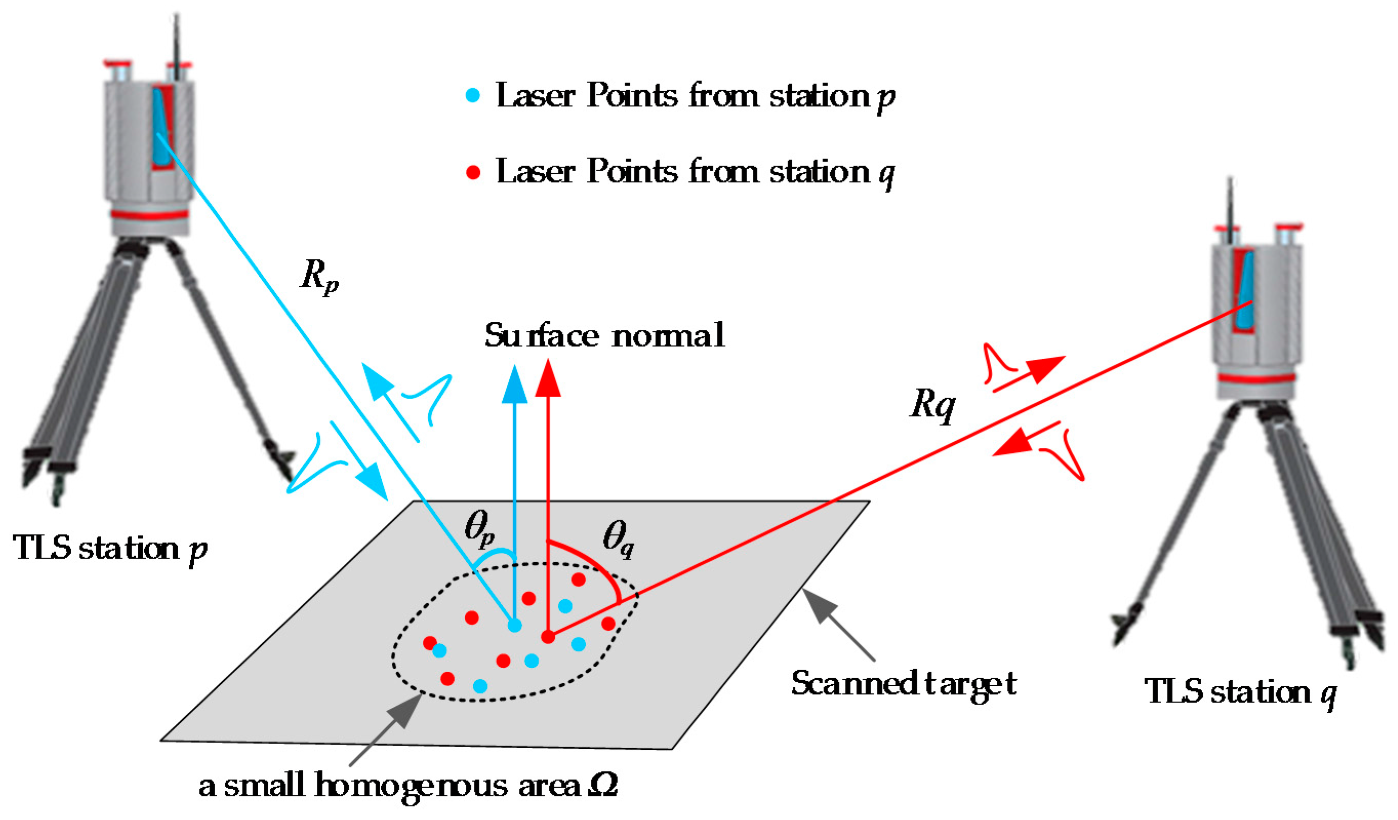
The estimation of the surface roughness parameter is important for the intensity correction. As the roughness parameter may differ greatly from object to object and from point to point even for the same kind of object, it should be estimated individually for each point of the object. Therefore, a new method to estimate the surface roughness parameter of the scanned object at each point individually is proposed in this paper, as shown in Figure 3.
Firstly, all the distance corrected intensity data sets and (i = 1, 2, …, M) were selected from the stations p and q, respectively, where M is the total number of laser points from the two stations in the same small homogenous area Ω. Secondly, to obtain the optimal value of the surface roughness parameter, all the distance corrected intensities from stations p and q are further corrected according to Equation (15) with the surface roughness parameter from 0° to 90° in a step interval of 1°. In the overlapped region, the corrected intensities of the homologous laser points from stations p and q should be the same and be expressed as
where and are the corrected intensities of the ith laser point from stations p and q in the same small homogenous area Ω, respectively. Owing to the impacts of the background noise and the measurement error of the TLS system, the corrected intensities and may slightly differ from each other. The difference can be written as
where i and M are the serial and total numbers of the laser points in the small homogenous area Ω. Then, the surface roughness parameter can be obtained by using the objective function O(ε), which is
where the objective function O(ε) is the root mean square value of the difference (i = 1, 2, …, M). The results of the objective function are calculated using the values of surface roughness parameter from 0° to 90° in a step interval of 1°. Thus, we can get 91 groups of results of the objective function, and the surface roughness parameter is selected as the value that minimizes the result of the objective function.
Once the surface roughness parameter is determined, it is substituted in Equation (9) to correct the intensity data for the entire dataset.
2.5. Retrieving Reflectance
After the distance and incident effects are eliminated, the intensity data mainly depends on the surface reflectance of the scanned object. The corrected intensity has a logarithmic relationship with the reflectance as
Thus, the reflectance can be obtained by
where the corrected intensity can be obtained from Equation (9) and the reflectance ρλ is expressed as a percentage.
To further validate the proposed method for TLS intensity correction, we used an FieldSpec®4 Hi-Res spectrometer (provided by Analytical Spectral Devices (ASD), Inc., Longmont, CO, USA) with the spectral resolution of 10 nm and wavelength accuracy of 0.5 nm [40] to measure the reflectance of the three kinds of objects. The reflectance values of the three kinds of objects measured by the spectrometer at the wavelength of 1550 nm were treated as the reference values. Each reference value was the mean of the reflectance values measured by the spectrometer at 10 equally spaced sample points on a homogeneous area of the corresponding kind of object.
3. Experiments and Data Acquisition
In this section, two sets of experiments were carried out to verify the proposed method. The first set is on intensity correction to distance effect only using three reference targets with various reflectance values. The second set is on intensity correction to both distance and incident angle effects using multi-station scans.
To obtain the coefficients in Equation (11), three reference targets with a size of 60 cm × 60 cm, Teflon material and reflectance of 15%, 30% and 60% were scanned by the TLS sensor at a series of distances from 5 m to 50 m. The TLS sensor utilized in this research is Riegl VZ-400i. The wavelength of Riegl VZ-400i is 1550 nm, the range accuracy is 5 mm, the angular resolution is better than 0.007°, and the diameter of the laser beam footprint is 35 mm @100 m [34]. Experimental setup and scene of the distance experiment are shown as Figure 4. To eliminate the incident angle effect on the intensity data, the incident angle was set to 0° during the scanning process. Each of the three reference targets was firstly scanned at the distance of 5 m, then moved forward at a step interval of 0.3 m until the distance reached 12 m. From the distance of 12 m, the reference targets were moved forward with a step interval of 1.2 m until the distance reached 50 m. For each reference target, intensity data of 50 laser points around the center of the reference target were obtained at each distance, and the means of the intensity data of the laser points were applied to eliminate the distance effect.
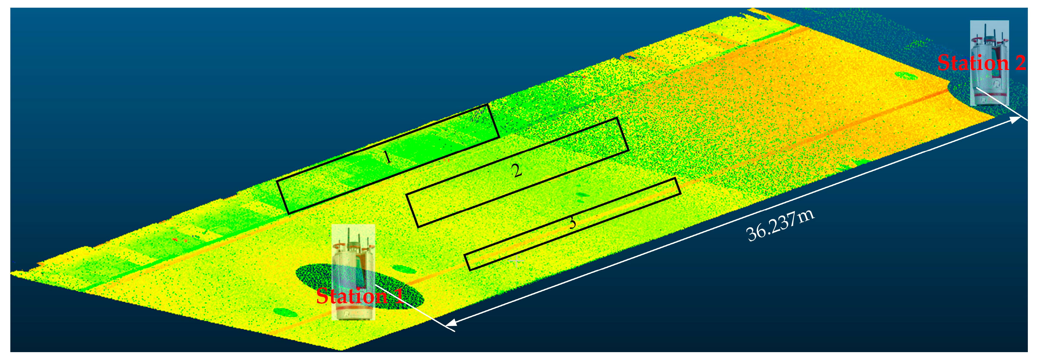
In order to estimate the surface roughness parameter and validate the feasibility of the proposed method, the second set of experiments was conducted to obtain multi-station scans. Before intensity correction, the multi-station scans were preprocessed and registered using the RiSCAN PRO software (v2.42, RIEGL Laser Measurement Systems GmbH, Vienna, Austria). In the registration process, some corresponding points from multi-station scans were selected manually to make coarse registration. Then the fine registration was completed using the Iterative Closest Point (ICP) algorithm [41]. Figure 5 is the point cloud of the multi-station scans after registration, which is colored with raw intensity data and displayed by the CloudCompare software (v2.9, D. Girardeau-Montaut, EDF Research and Development, Telecom Paris Tech, Paris, France) [42]. It consists of three kinds of objects including paving brick, concrete road and marking line, which are numbered as 1, 2 and 3, respectively.
4. Results
4.1. Results of Distance Effect Correction
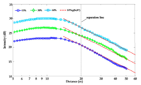
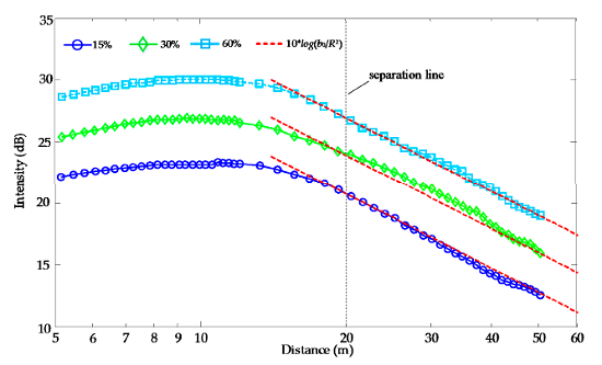
To implement the intensity correction, the distance effect should be first corrected. The variations of raw intensity data with distance for the three reference targets are shown in Figure 6. We can see that the raw intensity data increases firstly with increase of the distance up to around 12 m for all the three reference targets. Then, the intensity decreases with increase of the distance until 50 m. When the distance is shorter than around 20 m, the system transmission factor, such as the brightness reducer or the receiver optics’ defocusing effect, has a significant effect on the raw intensity data, and it makes that the intensity data dissatisfy the radar range equation (refer to Equation (4)). When the distance is longer than around 20 m, the distance effect is the main factor that influences the raw intensity data and other effects can be ignored or remain unchanged with distance. Thus, we can see that the intensity data of each of the three reference targets is proportional to 10 × log(b0/R2) when the distance is longer than 20 m, which meets the radar range equation. Therefore, the separation point is selected as Rsep = 20 m in this research.
The intensity data within a short distance range, less than 20 m, were fit by the nonlinear least square estimation, and the fitting results relative to the polynomial order (n) of the function are shown in Figure 7.
In the polynomial fitting process, the RMS values of fitting errors and coefficient of determination (R-square) are used to evaluate the influence of polynomial order (n) on the fitting results in this paper. From Figure 7, we know that when the value of polynomial order is larger than 3, the R-square and RMS values of fitting errors remain almost unchanged. Moreover, the R-square is 0.962 and very close to 1, and the RMS value is only 0.261 dB at the polynomial order of 3. Therefore, the optimal order of the polynomial function was selected as n = 3. According to the continuity of the function, the coefficient b0 of the function can be calculated as b0 = 3.218 × 10⁵ using Equations (11) and (12). After the fitting process, the two segments of were obtained and expressed as
After calculating for all the intensity data, the RMS value of fitting errors of the polynomial model is 0.296 dB, and the R-square is 0.984, which is very close to 1. Therefore, the polynomial model has a good fitting result.
4.2. Results of Incident Angle Effect Correction
Assume that Lin = 1, the simulated results of the Oren–Nayar model for different surface roughness parameters are shown in Figure 8. For flat surfaces without facet variation, i.e., ε = 0°, the Oren–Nayar model is equal to the Lambertian model, shown in the blue curve of Figure 8. From the results of Figure 8a, we know that the normalized intensity data decreases with the increase of the incident angle, and it also decreases with the increase of ε at the same time for incident angle less than about 50°. However, for incident angle larger than about 50°, it increases with the increase of ε at the same incident angle. Furthermore, the absolute deviations of from decrease firstly and then increase with the increase of the incident angle, as shown in Figure 8b. It shows that the deviation is as large as 0.4 for the surface roughness parameter ε of 60°, even for the small surface roughness parameter ε of 15°, and the deviation also reaches up to 0.2. Thus, the surface roughness parameter has a large effect on the intensity data. Moreover, the rougher the surface of the scanned object, the more significant the deviation of the Oren–Nayar model from the Lambertian model. Only if the incident angle is around in the interval [35°, 50°], the deviation is small, less than 0.05, as shown in the red box of Figure 8b.
As mentioned, we know that the surface roughness parameter is crucial for intensity correction, and different surface roughness parameter will generate different correction results for the same object. When the Lambertian model is used to correct the intensity data, the surface roughness parameter cannot be involved, resulting in correction results deviating greatly from the real intensity data that depend on the physical characteristic of the scanned objects. Only when the surface roughness parameter is considered can the corrected intensity data better approach the real intensity data. Therefore, the surface roughness parameter should be estimated for each kind of object before being used for intensity correction.
To eliminate the incident angle effect on the TLS intensity data, the surface roughness parameter of the three kinds of objects should be determined according to Equations (17) and (18). The results are shown in Table 1. It can be seen that the three kinds of objects have different surface roughness parameter, the means of which are 20.6°, 17.9° and 20.8°, respectively. The mean and standard deviation (Std.) of surface roughness parameter of the paving brick, concrete road and marking line are large. The divergence of the surface roughness parameter of each of the three kinds of objects indicates that the surface roughness parameter differs from position to position even for the same kind of object. Therefore, the surface roughness parameter of the same kind of object should be estimated individually from point to point.
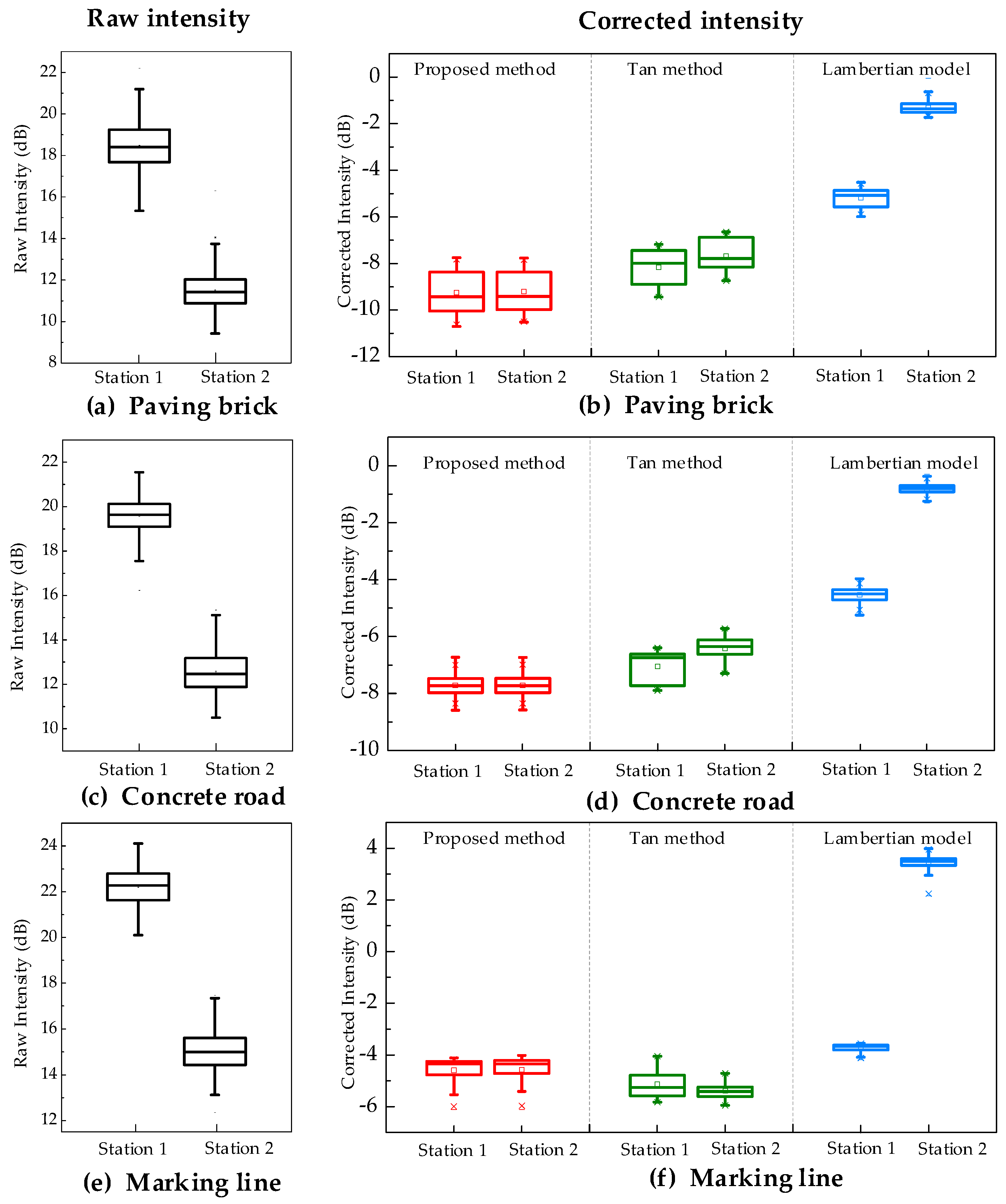
In order to eliminate the distance and incident angle effects on intensity data, three methods were used to correct the raw intensity data in this research, including the proposed method, the Tan method [7] and the Lambertian model. In the Tan method, the distance effect is eliminated by reference targets not using the distance effect function and the surface roughness parameter is estimated by using the average surface roughness parameter of 20 manually selected points for each kind of object. However, in the proposed method, the local surface roughness is estimated from point to point by using the intensity data of corresponding points in the overlapped regions of two stations, rather than being estimated by averaging the surface roughness at 20 manually selected points for each kind of object. The distributions of raw and corrected intensity data for the three kinds of objects from TLS stations 1 and 2 are shown in Figure 9.
Firstly, it can be seen that, as the incident angle and distance in station 1 are different from those in station 2, the raw intensity data of all the three kinds of objects in station 1 are significantly different from those in station 2. The differences of the distribution of raw intensity between stations 1 and 2 are as large as 7 dB for the three kinds of objects, and the distribution widths are from 4 dB to 7 dB for the three kinds of objects in stations 1 and 2. However, the distribution of corrected intensity between stations 1 and 2 are almost the same, and the distribution widths are less than 3 dB for the three kinds of objects. Therefore, the raw intensity data should be corrected before used.
Secondly, after being corrected by the Lambertian model, the distributions of corrected intensity data of all the three kinds of objects from station 1 still differ greatly from those from station 2. Especially for the marking line, the difference of distributions of the corrected intensity data between stations 1 and 2 is as large as 6 dB. After being corrected by the Tan method, the distributions of intensity data are better than those corrected by the Lambertian model. However, the difference still exists between the distributions of intensity data from stations 1 and 2.
Compared with the distributions of intensity data corrected by the other two methods, the distributions of intensity data corrected by the proposed method from station 1 are almost the same as those from station 2 for all the three kinds of objects. Therefore, the correction accuracy using the proposed method is better than those using the other two methods.
4.3. Reflectance Retrieved from Corrected Intensity Data
The means and standard deviations of the reflectance values for the three kinds of objects obtained by the spectrometer, the proposed method, the Tan method and the Lambertian model are shown in Table 2. From the results, it can be seen that the deviations of the mean reflectance values obtained by Lambertian model from those obtained by the spectrometer are larger than 37%. The deviations of the mean reflectance values obtained by the Tan method from those obtained by the spectrometer are 6.2%, 6.7% and −6.0% for the three kinds of objects, respectively. The deviations of the mean reflectance values obtained by the proposed method from those obtained by the spectrometer are 1.0%, 2.5% and −0.8% for the three kinds of objects, respectively, and the standard deviations of the reflectance values obtained by the proposed method are close to those obtained by the spectrometer. The mean reflectance values retrieved from the proposed method for all three kinds of objects are closer to the reference values than those retrieved from the Tan method and Lambertian model. Overall, we can say that the proposed method is better than the Tan method and provides higher accuracy reflectance of the scanned object.
5. Discussion
In this study, the intensity correction combining the piecewise fitting and overlap-driven adjustment approaches has been carried out for TLS. Results of the distance experiment performed with three different reflectance targets demonstrated that the intensity values recorded by the used TLS sensor cannot follow the 1/R2 relation at near distance, which is consistent with some previous studies [6,20]. However, at far distance (about 20 m) the intensity values are proportional to the range (1/R2), which overcomes the technical issue of defocusing on TLS instruments. Thus, the distance effect function is established using the piecewise fitting approach. The incident angle effect function is established using the Oren–Nayar model that employs the surface roughness parameter of the scanned object. The distance effect and incidence angle effect on intensity data are corrected independently as previous studies suggested [7,33].
Results of incident angle effect correction show that as the surface roughness parameter of the three kinds of objects are large, their surface characteristics do not meet the Lambertian model, and intensity correction using the Lambertian model generates large deviations. Therefore, the Lambertian model is not suitable for the intensity correction of the scanned object with a large surface roughness parameter, and not as good as the Tan method. For the marking line, the surface roughness parameter and the difference of incident angles between stations 1 and 2 are both large so that the intensity correction using the Lambertian model generates large deviation. If the surface of scanned object is homogenous and has no inhomogeneous points, such as crack points, contaminants and pits, the Tan method is suitable and can eliminate the random measurement error of the TLS sensor through the 20 manually selected points for each kind of object. However, the scanned object often has structural damage or contaminants on its surface in the real condition. When the manually selected points include inhomogeneous points, the estimation of surface roughness parameter will generate a large deviation that can further affect the following intensity correction. As the local surface roughness parameter of the scanned object is estimated using the intensity data of a small area around the corresponding point in the overlapped region of the multi-station scans in the proposed method, the estimation of the local surface roughness parameter at each point is not affected by the inhomogeneous points at other positions of the scanned object like the Tan method, and hence more accurate. Therefore, the proposed method can improve the correction accuracy of intensity data and obtain more accurate reflectance for the three kinds of objects than that derived from the Tan method.
The advantage of the proposed method is that the local surface roughness parameter is considered in TLS intensity correction and estimated by using the intensity data of the corresponding points in the overlapped regions of multi-station scans, where there is no need to manually select the homogenous points as the Tan method described therein. Moreover, because the points selected manually in the Tan method can include inhomogeneous points, the estimation of surface roughness parameter will generate a larger deviation that can further affect the following intensity correction. Thus, the proposed method for TLS intensity correction is better than the Tan method. However, the proposed method for the intensity correction seems to have some limitations. First, the proposed method cannot be used to well correct the intensity data for the objects with glossy surfaces, especially when the incident angle is 0°. Because the Oren–Nayar is a physical model, which only considers the diffuse reflection, without the specular reflection. Although mostly natural objects meet the Oren–Nayar model, the objects with smooth or glossy surfaces, such as the glasses and glazed tile, cannot meet the Oren–Nayar model. Second, the proposed method is not suitable for a long-range TLS. As the size of laser footprint is large for the long-range TLS, the small homogenous area between two stations hardly exists and even the laser footprint is larger than the scanned object.
6. Conclusions
In this study, a new method was proposed to correct the intensity data for TLS by combining the piecewise fitting and overlap-driven adjustment approaches. In the method, the local surface roughness parameter is estimated from point to point by using the intensity data of corresponding points in the overlapped regions of multi-station scans, rather than being estimated by averaging the surface roughness parameter at 20 manually selected points for each kind of object in the Tan method. Our method estimating the local surface roughness parameter is not influenced by the inhomogeneous points, whereas the Tan method is affected by the inhomogeneous points due to selecting the points at different positions on the scanned object. Thus, the estimation using the proposed method is more accurate than that using the Tan method.
The experimental results demonstrate that the distribution of corrected intensity data between stations 1 and 2 are almost the same, and the distribution widths of corrected intensity data are reduced to 3 dB compared with the distribution width of 7 dB for raw intensity data. The reflectance values derived from the proposed method are much closer to the reference values obtained by the spectrometer than those derived from the Tan method, and the reflectance deviations are all less than 3% for the three kinds of objects. It proves that the proposed method can improve the correction accuracy of intensity data, and hence be better applied for building classification, structural damage detection and road traffic marking identification.
Acknowledgments
This research work is supported in part by the National Natural Science Foundation of China (NSFC) (61671038), Fundamental Research Funds for the Central Universities (YWF-16-BJ-Y-54, YWF-17-BJ-Y-20), and the Excellence Foundation of Beihang University (BUAA) for PhD Students (2017058). The authors would like to gratefully acknowledge the Riegl agency (Five-star Electronic Technology Company Limited) who provided us with the instrument RIEGL VZ-400i.
Author Contributions
Teng Xu designed the method and wrote the manuscript. Lijun Xu and Xiaolu Li provided the overall conception of this research and revised the manuscript. Junen Yao conducted the experiments and analyzed the experimental results. Teng Xu and Bingwei Yang completed all the experiments together.
Conflicts of Interest
The authors declare no conflict of interest.
References
- Kasperski, J.; Delacourt, C.; Allemand, P.; Potherat, P.; Jaud, M.; Varrel, E. Application of a terrestrial laser scanner (TLS) to the study of the Séchilienne Landslide (Isère, France). Remote Sens. 2010, 2, 2785–2802. [Google Scholar] [CrossRef]
- Liang, X.; Kankare, V.; Hyyppä, J.; Wang, Y.; Kukko, A.; Haggrén, H.; Yu, X.; Kaartinen, H.; Jaakkola, A.; Guan, F.; et al. Terrestrial laser scanning in forest inventories. ISPRS J. Photogramm. Remote Sens. 2016, 115, 63–67. [Google Scholar] [CrossRef]
- Pu, S.; Vosselman, G. Automatic extraction of building features from terrestrial laser scanning. Int. Arch. Photogramm. Remote Sens. Spat. Inf. Sci. 2006, 36, 25–27. [Google Scholar]
- Pu, S.; Vosselman, G. Extracting Windows from Terrestrial Laser Scanning. In Proceedings of the ISPRS Workshop ‘Laser Scanning 2007 and SilviLaser 2007’, Espoo, Finland, 12–14 September 2007; pp. 320–325. [Google Scholar]
- Boulaassal, H.; Landes, T.; Grussenmeyer, P. Automatic extraction of planar clusters and their contours on building facades recorded by terrestrial laser scanner. Int. J. Archit. Comput. 2009, 7, 1–20. [Google Scholar]
- Kaasalainen, S.; Jaakkola, A.; Kaasalainen, M.; Krooks, A.; Kukko, A. Analysis of incidence angle and distance effects on terrestrial laser scanner intensity: Search for correction methods. Remote Sens. 2011, 3, 2207–2221. [Google Scholar] [CrossRef]
- Tan, K.; Cheng, X.; Cheng, X. Modeling hemispherical reflectance for natural surfaces based on terrestrial laser scanning backscattered intensity data. Opt. Express 2016, 24, 22971–22988. [Google Scholar] [PubMed]
- Kashani, A.G.; Olsen, M.J.; Parrish, C.E.; Wilson, N. A review of LiDAR radiometric processing: From ad hoc intensity correction to rigorous radiometric calibration. Sensors 2015, 15, 28099–28128. [Google Scholar] [PubMed]
- Burton, D.; Dunlap, D.B.; Wood, L.J.; Flaig, P.P. Lidar intensity as a remote sensor of rock properties. J. Sediment. Res. 2011, 81, 339–347. [Google Scholar] [CrossRef]
- Olsen, M.J.; Kuester, F.; Chang, B.J.; Hutchinson, T.C. Terrestrial laser scanning-based structural damage assessment. J. Comput. Civ. Eng. 2010, 24, 264–272. [Google Scholar]
- Zhu, X.; Wang, T.; Darvishzadeh, R.; Skidmore, A.K.; Niemann, K.O. 3D leaf water content mapping using terrestrial laser scanner backscatter intensity with radiometric correction. ISPRS J. Photogramm. Remote Sens. 2015, 110, 14–23. [Google Scholar] [CrossRef]
- Guan, H.; Li, J.; Yu, Y.; Wang, C.; Chapman, M.; Yang, B. Using mobile laser scanning data for automated extraction of road markings. ISPRS J. Photogramm. Remote Sens. 2014, 87, 93–107. [Google Scholar] [CrossRef]
- López-Moreno, J.I.; Revuelto, J.; Alonso-Gonzáles, E.; Sanmiguel-Vallelado, A.; Fassnacht, S.R.; Deems, J.; Morán-Tejeda, E. Using very long-range terrestrial laser scanning to analyze the temporal consistency of the snowpack distribution in a high mountain environment. J. Mt. Sci. 2017, 14, 823–842. [Google Scholar] [CrossRef]
- Prokop, A. Assessing the applicability of terrestrial laser scanning for spatial snow depth measurements. Cold Reg. Sci. Technol. 2008, 54, 155–163. [Google Scholar] [CrossRef]
- Schwalbe, E.; Maas, H.G.; Dietrich, R.; Ewert, H. Glacier velocity determination from multitemporal terrestrial long range laser scanner point clouds. Int. Arch. Photogramm. Remote Sens. Spat. Inf. Sci. 2008, 5, 457–462. [Google Scholar]
- Song, J.H.; Han, S.H.; Yu, K.Y.; Kim, Y.I. Assessing the possibility of land-cover classification using LIDAR intensity data. Int. Arch. Photogramm. Remote Sens. Spat. Inf. Sci. 2002, 34, 259–262. [Google Scholar]
- Brennan, R.; Webster, T.L. Object-oriented land cover classification of lidar-derived surfaces. Can. J. Remote Sens. 2006, 32, 162–172. [Google Scholar] [CrossRef]
- Watt, P.; Wilson, J. Using airborne light detection and ranging to identify and monitor the performance of plantation species mixture. In Proceedings of the ForestSat, Borås, Sweden, 31 May–3 June 2005; pp. 51–55. [Google Scholar]
- Jutzi, B.; Gross, H. Normalization of LiDAR intensity data based on range and surface incidence angle. Int. Arch. Photogramm. Remote Sens. Spat. Inf. Sci. 2009, 38, 213–218. [Google Scholar]
- Fang, W.; Huang, X.; Zhang, F.; Li, D. Intensity correction of terrestrial laser scanning data by estimating laser transmission function. IEEE Trans. Geosci. Remote Sens. 2015, 53, 942–951. [Google Scholar] [CrossRef]
- Höfle, B.; Pfeifer, N. Correction of laser scanning intensity data: Data and model-driven approaches. ISPRS J. Photogramm. Remote Sens. 2007, 62, 415–433. [Google Scholar] [CrossRef]
- Tan, K.; Cheng, X. Correction of incidence angle and distance effects on TLS intensity data based on reference targets. Remote Sens. 2016, 8, 251. [Google Scholar] [CrossRef]
- Tan, K.; Cheng, X. Specular reflection effects elimination in terrestrial laser scanning intensity data using Phong model. Remote Sens. 2017, 9, 853. [Google Scholar] [CrossRef]
- Minnaert, M. The reciprocity principle in lunar photometry. Astrophys. J. 1941, 93, 403–410. [Google Scholar] [CrossRef]
- Henyey, L.; Greenstein, J. Diffuse radiation in the galaxy. Astrophys. J. 1941, 93, 70–83. [Google Scholar] [CrossRef]
- Franceschi, M.; Teza, G.; Preto, N.; Pesci, A.; Galgaro, A.; Girardi, S. Discrimination between marls and limestones using intensity data from terrestrial laser scanner. ISPRS J. Photogramm. Remote Sens. 2009, 64, 522–528. [Google Scholar] [CrossRef]
- Kaasalainen, S.; Kukko, A.; Lindroos, T.; Litkey, P.; Kaartinen, H.; Hyyppa, J.; Ahokas, E. Brightness measurements and calibration with airborne and terrestrial laser scanners. IEEE Trans. Geosci. Remote Sens. 2008, 46, 528–534. [Google Scholar] [CrossRef]
- Korpela, I.; Ørka, H.O.; Hyyppä, J.; Heikkinen, V.; Tokola, T. Range and AGC normalization in airborne discrete-return LiDAR intensity data for forest canopies. ISPRS J. Photogramm. Remote Sens. 2010, 65, 369–379. [Google Scholar] [CrossRef]
- Biavati, G.; Donfrancesco, G.D.; Cairo, F.; Feist, D.G. Correction scheme for close range lidar returns. Appl. Opt. 2011, 50, 5872–5882. [Google Scholar] [CrossRef] [PubMed]
- Wagner, W. Radiometric calibration of small-footprint full-waveform airborne laser scanner measurements: Basic physical concepts. ISPRS J. Photogramm. Remote Sens. 2010, 65, 505–513. [Google Scholar] [CrossRef]
- Wagner, W.; Ullrich, A.; Ducic, V.; Melzer, T.; Studnicka, N. Gaussian decomposition and calibration of a novel small-footprint full-waveform digitising airborne laser scanner. ISPRS J. Photogramm. Remote Sens. 2006, 60, 100–112. [Google Scholar] [CrossRef]
- Carrea, D.; Abellan, A.; Humair, F.; Matasci, B.; Derron, M.H.; Jaboyedoff, M. Correction of terrestrial LiDAR intensity channel using Oren–Nayar reflectance model: An application to lithological differentiation. ISPRS J. Photogramm. Remote Sens. 2016, 113, 17–29. [Google Scholar] [CrossRef]
- Krooks, A.; Kaasalainen, S.; Hakala, T.; Nevalainen, O. Correction of intensity incidence angle effect in terrestrial laser scanning. ISPRS Ann. Photogramm. Remote Sens. Spat. Inf. Sci. 2013, 2, 145–150. [Google Scholar] [CrossRef]
- Datasheet RIEGL VZ-400i. 2017. Available online: http://www.riegl.com/uploads/tx_pxpriegldownloads/RIEGL_VZ-400i_Datasheet_2017-09-08.pdf (accessed on 24 October 2017).
- Pfennigbauer, M.; Ullrich, A. Improving quality of laser scanning data acquisition through calibrated amplitude and pulse deviation measurement. Proc. SPIE 2010, 7684. [Google Scholar] [CrossRef]
- Oren, M.; Nayar, S.K. Generalization of Lambert’s reflectance model. In Proceedings of the 21st Annual Conference on Computer Graphics and Interactive Techniques, Orlando, FL, USA, 24–29 July 1994; pp. 239–246. [Google Scholar]
- Hapke, B. Theory of Reflectance and Emittance Spectroscopy; Cambridge University Press: Cambridge, UK, 1993. [Google Scholar]
- Poullain, E.; Garestier, F.; Levoy, F.; Bretel, P. Analysis of ALS intensity behavior as a function of the incidence angle in coastal environments. IEEE J. Sel. Top. Appl. Earth Obs. Remote Sens. 2016, 9, 313–325. [Google Scholar] [CrossRef]
- Hasegawa, H. Evaluations of LiDAR reflectance amplitude sensitivity towards land cover conditions. Bull. Geogr. Surv. Inst. 2006, 53, 43–50. [Google Scholar]
- FieldSpec 4 Hi-Res Spectroradiometer. Available online: https://www.asdi.com/products-and-services/fieldspec-spectroradiometers/fieldspec-4-hi-res (accessed on 24 October 2017).
- Besl, P.J.; McKay, N.D. A method for registration of 3-D shapes. IEEE Trans. Pattern Anal. Mach. Intell. 1992, 14, 239–256. [Google Scholar] [CrossRef]
- Girardeau-Montaut, D. Cloudcompare, a 3D Point Cloud and Mesh Processing Free Software. EDF R&D, Telecom ParisTech, 2014. Available online: www.danielgm.net/cc (accessed on 24 October 2017).
- Legend for Box Chart Components. Available online: http://www.originlab.com/doc/Origin-Help/box-legend (accessed on 24 October 2017).
Figure 1.
Reflected light of a laser footprint on a perfect diffuse target is uniformly scattered into a hemisphere.
Figure 1.
Reflected light of a laser footprint on a perfect diffuse target is uniformly scattered into a hemisphere.
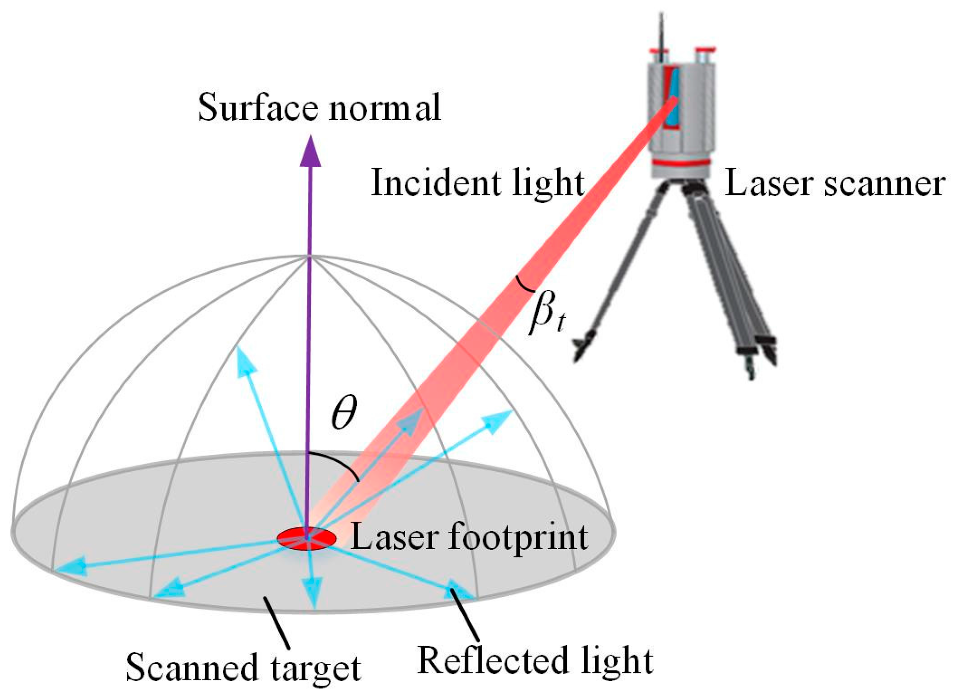
Figure 2.
Geometrics of terrestrial laser scanning (TLS) for calculating the distance R and the incident angle θ, where O-XYZ is the user coordinate system, the 3D coordinates of points D and Os are defined as (x, y, z) and (x0, y0, z0).
Figure 2.
Geometrics of terrestrial laser scanning (TLS) for calculating the distance R and the incident angle θ, where O-XYZ is the user coordinate system, the 3D coordinates of points D and Os are defined as (x, y, z) and (x0, y0, z0).
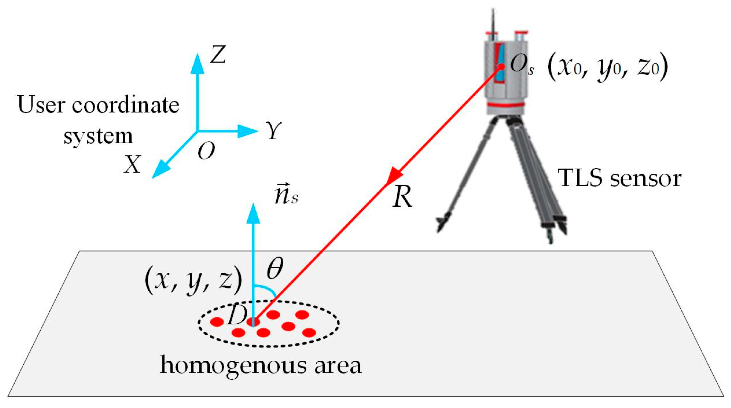
Figure 3.
Schematic diagram of the proposed method to estimate the optimal value of the surface roughness parameter using the intensity data from TLS stations p and q in a small homogenous area Ω. Rp and Rq are the distances from laser points to TLS stations p and q, respectively. θp and θq are the incident angles between the surface normal and the incident lights from TLS station p and q, respectively.

Figure 4.
Experimental setup and scene of the distance experiment. (a) experimental setup including Riegl VZ-400i and three reference targets with reflectance of 15%, 30% and 60%, respectively; (b) scene of the distance experiment with distance from 5 m to 50 m, and a step interval of 0.3 m from 5 m to 12 m, and 1.2 m from 12 m to 50 m, respectively.
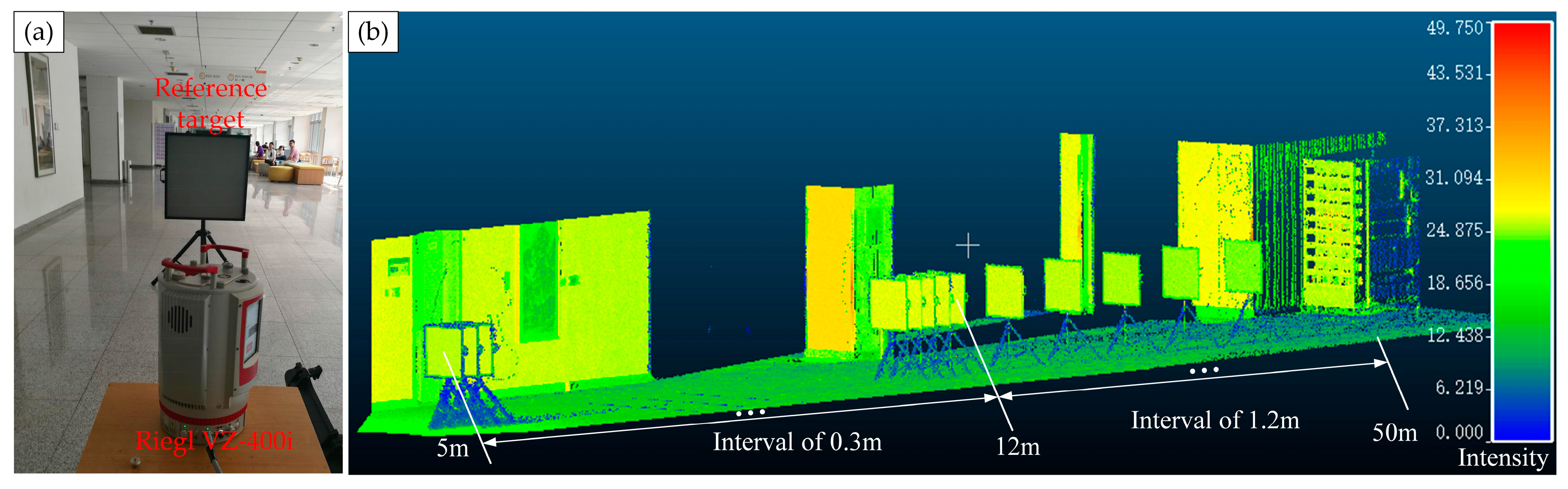
Figure 5.
Point cloud of the multi-station scans colored with raw intensity data. (Note that Nos. 1, 2 and 3 represent the paving brick, concrete road and marking line, respectively. The distance between the center of station 1 and station 2 is 36.237 m).
Figure 5.
Point cloud of the multi-station scans colored with raw intensity data. (Note that Nos. 1, 2 and 3 represent the paving brick, concrete road and marking line, respectively. The distance between the center of station 1 and station 2 is 36.237 m).

Figure 6.
Variation of raw intensity data with distance for all of the three reference targets with the reflectance of 15%, 30% and 60% at the incident angle of 0°.
Figure 6.
Variation of raw intensity data with distance for all of the three reference targets with the reflectance of 15%, 30% and 60% at the incident angle of 0°.
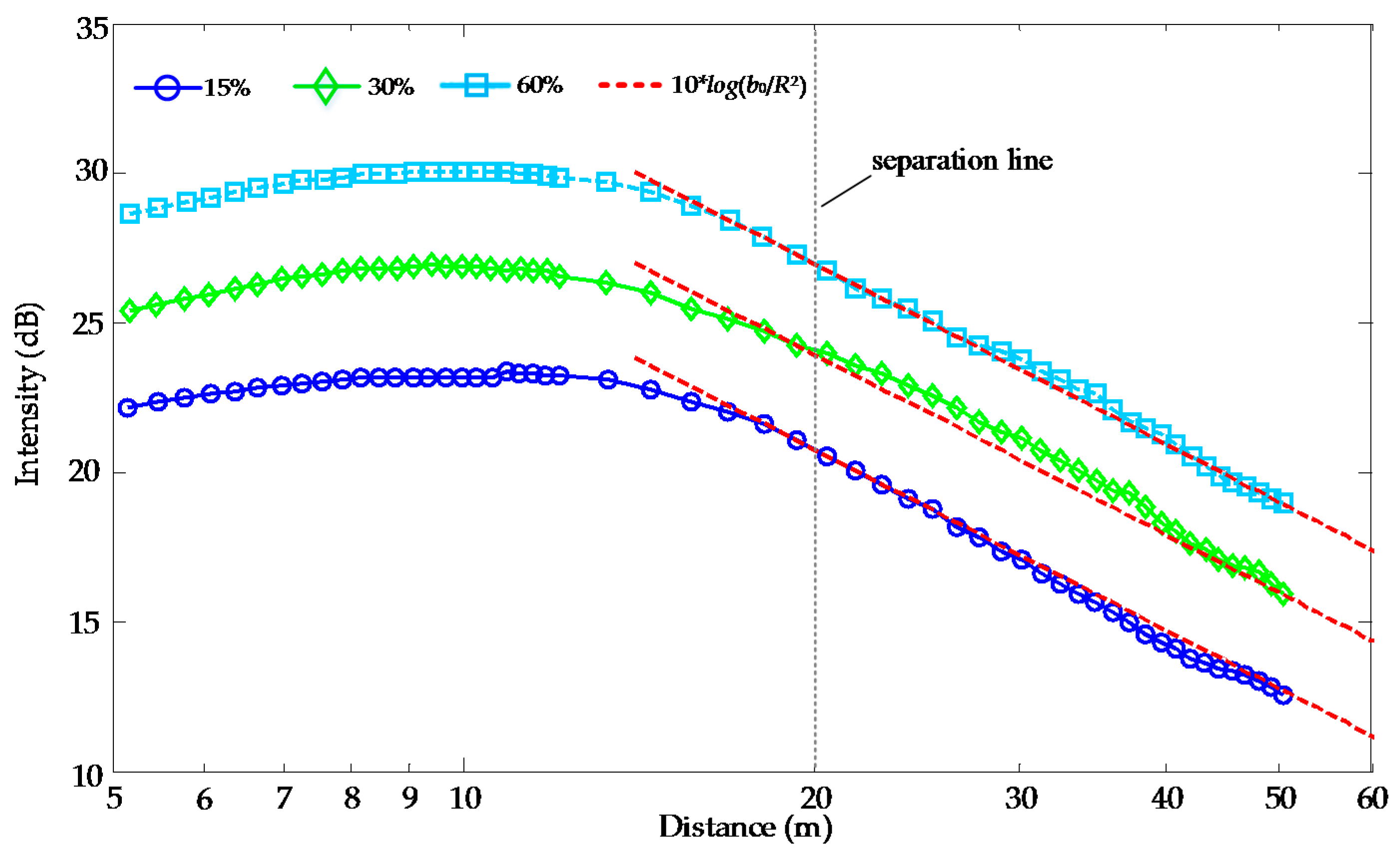
Figure 7.
Variation of fitting results with the polynomial order (n). (a) root-mean-square (RMS) values of the fitting errors varied with the polynomial order; (b) coefficient of determination (R-square) varied with the polynomial order.
Figure 7.
Variation of fitting results with the polynomial order (n). (a) root-mean-square (RMS) values of the fitting errors varied with the polynomial order; (b) coefficient of determination (R-square) varied with the polynomial order.
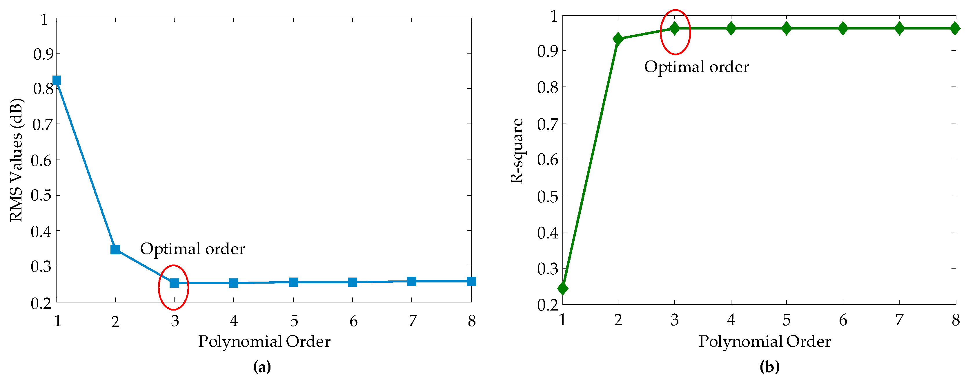
Figure 8.
Simulated results of Oren–Nayar model vs. Lambert model. (a) normalized intensity data for different surface roughness parameters; (b) absolute deviations of from .
Figure 8.
Simulated results of Oren–Nayar model vs. Lambert model. (a) normalized intensity data for different surface roughness parameters; (b) absolute deviations of from .
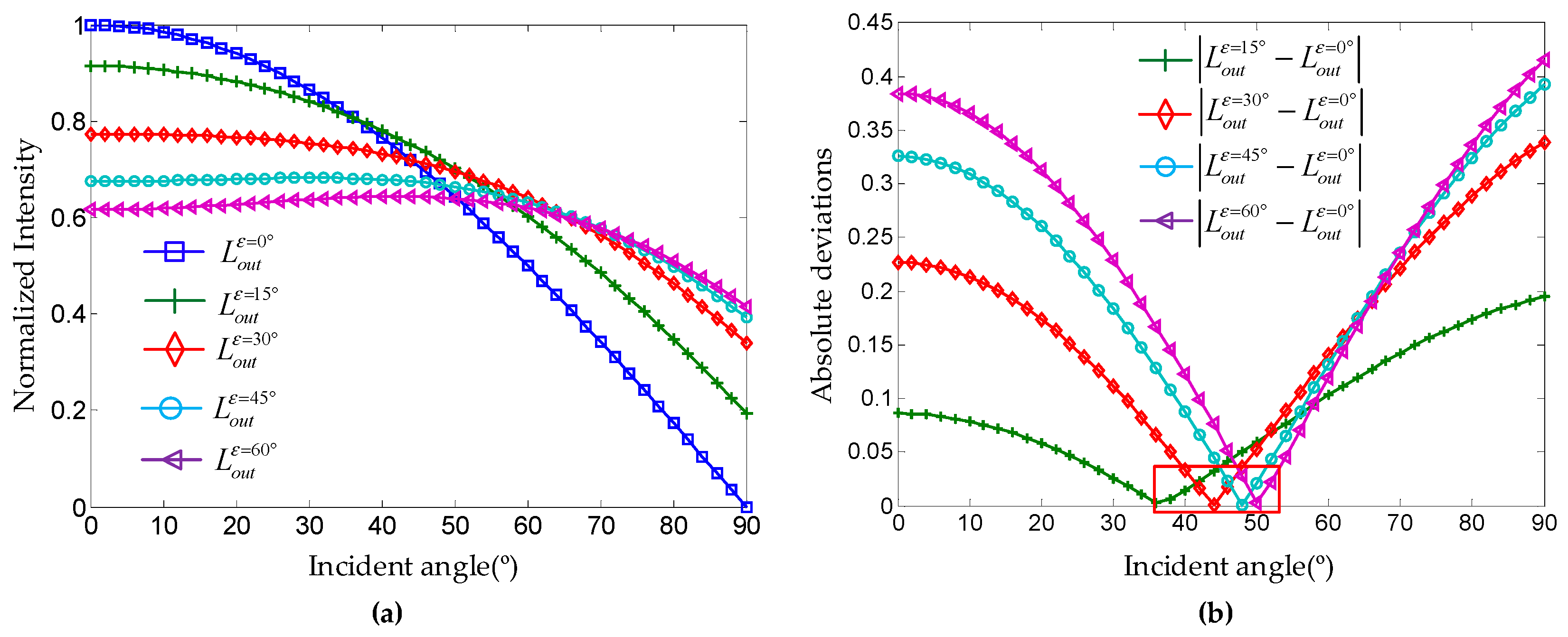
Figure 9.
Distributions of raw and corrected intensity data for the three kinds of objects from TLS stations 1 and 2. (a,c,e) are the distributions of raw intensity data for paving brick, concrete road and marking line, respectively; (b,d,f) are the distributions of intensity data corrected by the three methods for paving brick, concrete road and marking line, respectively. (For the box chart, the three long horizontal lines represent the lower quartile, median and upper quartile from down to up, respectively. The small circle represents the mean value. The two short horizontal lines are the lower whisker and upper whisker of the box, respectively. The two signs ‘x’ at both ends represent the 1% and 99% range of the box [43]).

Table 1.
Surface roughness parameter of the three kinds of objects.
| Surface Roughness Parameter | Paving Brick | Concrete Road | Marking Line |
|---|---|---|---|
| Mean | 20.6° | 17.9° | 20.8° |
| Std. | 2.6° | 2.3° | 2.8° |
Table 2.
Comparison of means and standard deviations (Std.) of the reflectance values of the three kinds of objects retrieved from the proposed method, the Tan method and the spectrometer.
Table 2.
Comparison of means and standard deviations (Std.) of the reflectance values of the three kinds of objects retrieved from the proposed method, the Tan method and the spectrometer.
| Methods | Paving Brick | Concrete Road | Marking Line | |||
|---|---|---|---|---|---|---|
| Mean | Std. | Mean | Std. | Mean | Std. | |
| the proposed method | 11.2% | 2.3% | 16.9% | 1.3% | 35.0% | 3.0% |
| Tan method | 16.4% | 2.9% | 20.8% | 1.9% | 29.8% | 2.4% |
| Lambertian model | 47.3% | 2.1% | 54.1% | 1.6% | 94.2% | 3.5% |
| Spectrometer | 10.2% | 1.9% | 14.4% | 1.5% | 35.8% | 2.8% |
© 2017 by the authors. Licensee MDPI, Basel, Switzerland. This article is an open access article distributed under the terms and conditions of the Creative Commons Attribution (CC BY) license (http://creativecommons.org/licenses/by/4.0/).
Share and Cite
MDPI and ACS Style
Xu, T.; Xu, L.; Yang, B.; Li, X.; Yao, J. Terrestrial Laser Scanning Intensity Correction by Piecewise Fitting and Overlap-Driven Adjustment. Remote Sens. 2017, 9, 1090. https://doi.org/10.3390/rs9111090
AMA Style
Xu T, Xu L, Yang B, Li X, Yao J. Terrestrial Laser Scanning Intensity Correction by Piecewise Fitting and Overlap-Driven Adjustment. Remote Sensing. 2017; 9(11):1090. https://doi.org/10.3390/rs9111090
Chicago/Turabian StyleXu, Teng, Lijun Xu, Bingwei Yang, Xiaolu Li, and Junen Yao. 2017. "Terrestrial Laser Scanning Intensity Correction by Piecewise Fitting and Overlap-Driven Adjustment" Remote Sensing 9, no. 11: 1090. https://doi.org/10.3390/rs9111090
Note that from the first issue of 2016, this journal uses article numbers instead of page numbers. See further details here.