Circa 2010 Land Cover of Canada: Local Optimization Methodology and Product Development

1
Natural Resources Canada, Canadian Centre for Remote Sensing, 560 Rochester, Ottawa, ON K1A 0E4, Canada
2
Environment and Climate Change Canada, Landscape Science and Technology, Ontario, 1125 Colonel By Drive, Ottawa, ON K1S 5B6, Canada
*
Author to whom correspondence should be addressed.
Remote Sens. 2017, 9(11), 1098; https://doi.org/10.3390/rs9111098
Submission received: 1 September 2017
/
Revised: 17 October 2017
/
Accepted: 25 October 2017
/
Published: 27 October 2017
(This article belongs to the Special Issue GIS and Remote Sensing advances in Land Change Science)
Abstract
:Land cover information is necessary for a large range of environmental applications related to climate impacts and adaption, emergency response, wildlife habitat, etc. In Canada, a 2008 user survey indicated that the most practical land cover data is provided in a nationwide 30 m spatial resolution format, with an update frequency of five years. In response to this need, the Canada Centre for Remote Sensing (CCRS) has generated a 30 m land cover map of Canada for the base year 2010, as the first of a planned series of maps to be updated every five years, or more frequently. This land cover dataset is also the Canadian contribution to the 30 m spatial resolution 2010 Land Cover Map of North America, which is produced by Mexican, American and Canadian government institutions under a collaboration called the North American Land Change Monitoring System (NALCMS). This paper describes the mapping approach used for generating this land cover dataset for Canada from Thematic Mapper (TM) and Enhanced Thematic Mapper (ETM+) Landsat sensor observations. The innovative part of the mapping approach is the local optimization of the land cover classifier, which has resulted in increased spatial consistency and accuracy. Training and classifying with locally confined reference samples over a large number of partially overlapping areas (i.e., moving windows) ensures the optimization of the classifier to a local land cover distribution, and decreases the negative effect of signature extension. A weighted combination of labels, which is determined by the classifier in overlapping windows, defines the final label for each pixel. Since the approach requires extensive computation, it has been developed and deployed using the Government of Canada’s High-Performance Computing Center (HPC). An accuracy assessment based on 2811 randomly distributed samples shows that land cover data produced with this new approach has achieved 76.60% accuracy with no marked spatial disparities.
Keywords:
land cover; land cover change; landsat; Canada; 2010; random forest algorithm; classification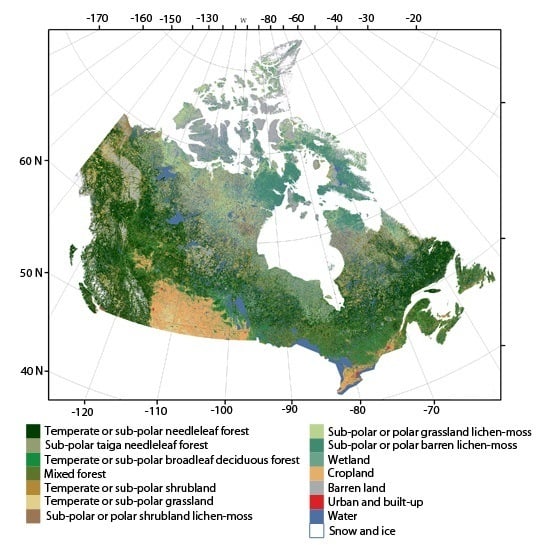
1. Introduction
National-scale land cover and land cover change information are required for studying land-surface processes that characterize environmental, social, and economic aspects of sustainability. The International Geosphere Biosphere Programme (IGBP), the World Climate Research Programme (WCRP), and global monitoring have long articulated the science requirement for land cover information, in particular at the global level. Land cover is a fundamental earth surface attribute shaped by geologic, hydrologic, climatic, atmospheric, and land-use processes occurring at a range of space–time scales. Land cover, in turn, affects these processes through feedback mechanisms such as plant respiration, which both absorbs and releases carbon, water, oxygen, and other biochemical elements from or to the environment. Therefore, knowledge of land cover is essential for understanding earth surface processes that are relevant for land management and the preservation of natural environments that may influence ecosystem and human health [1].
Global and continental land cover information is needed to implement various United Nations’ initiatives: the Millennium Development Goals (MDG), the Framework Convention on Climate Change (FCCC), the Convention on Biological Diversity (CBD), the Convention to Combat Desertification (CCD) and the Forum on Forest (UNFF). A list of Essential Climate Variables (ECV) endorsed by the Global Climate Observing System (GCOS) and Committee on Earth Observation Satellites (CEOS) science community includes land cover as an essential terrestrial variable [2,3,4]. The GCOS-107 [2] report, which defines key requirements for ECV-land cover, recommends annual updates at 0.25–1 km, and five-year updates at 10–30 m spatial resolution.
In Canada, a number of national land cover products have been generated using medium and low-resolution (250 m–1 km) optical satellite data, including data acquired by the Moderate Resolution Imagining Spectroradiometer (MODIS), the Satellite Pour l’Observation de la Terre (SPOT VEGETATION), and the Advance Very High-Resolution Radiometer (AVHRR) sensors [5,6,7]. More recent land cover information over Canada has been generated by the Canada Centre for Remote Sensing (CCRS) under the North American Land Change Monitoring System (NALCMS) collaboration. NALCMS is a collaborative framework involving CCRS’ parent organization, Natural Resources Canada (NRCan); the United States Geological Survey (USGS); and Mexican institutions including the National Institute of Statistics and Geography (INEGI), the National Forestry Commission (CONAFOR), and the National Commission for Knowledge and Use of Biodiversity (CONABIO). The collective need for a harmonized land cover monitoring system across North America’s political boundaries was a motivating factor for establishing the NALCMS collaboration. The NALCMS group has used national land cover mapping efforts to assemble continental land cover and change maps for North America from MODIS observations at 250 m spatial resolution for 2005 and 2010 [8,9]. The current NALCMS effort is to generate cross-border synchronized 30 m land cover of the North America continent for the year 2010. The 2010 baseline map will be used for generating a land cover time series following the updating approach described in Latifovic and Pouliot [10]. To ensure continuity with the existing 2005–2010 time series at 250 m, the new time series at 30 m will start from 2010, ensuring overlap that meets minimal requirements for data continuity. As with the 250 m maps, this 30 m map is being compiled from national land cover mapping efforts.
In support of creation of this circa 2010 North American Land Cover, the objective of the study was to develop a semi-automated classification approach to improve the accuracy and consistency of the new land cover map of Canada generated from Landsat Thematic Mapper (TM) and Enhanced Thematic Mapper (ETM+) observations at 30 m. Thus, this paper describes both the mapping approach with local classifier optimization, and the characteristics of the produced map.
2. Materials and Methods
2.1. Landsat Data and Processing
The initial data coverage of Canada includes 13,350 Landsat TM/ETM+ scenes all obtained from the United States (US) Geological Survey. Scenes spanned the 2009–2011 period, and were all acquired in July and August. The procedure to create a full coverage of Canada includes: re-projection, calibration, cloud/cloud shadow detection, compositing, and additional corrections as described by Latifovic et al. [11]. The Landsat mosaic of Canada July–August circa 2010 is shown in Figure 1. This mosaic was used to generate the land cover dataset described in this article. In order to reduce significant phenological differences due to strong vegetation gradients, particularly south–north, a narrow acquisition window of July–August 2010 was selected. However, such a short period does not provide clear-sky coverage over Canada. A compromise was made by including two more July–August periods from adjacent years, 2009 and 2011. Selecting adjacent pixels from different years could create inconsistencies over areas where land cover changes occurred in the 2009–2011 period and adjacent pixels were selected from different years (i.e., before and after changes). To minimize this, selection criteria were adjusted to preferentially select observations from 2010 over no change areas, and from 2011 over changed areas. Overall, 10% of observations were selected from 2009, 70% were from 2010, and 20% were from 2011. For each pixel, a scene ID with the time of acquisition is provided as a separate layer. When this product is used for studies involving temporal aspects, the provided time information may need to be considered. Processing was performed using a tile system to facilitate parallel processing and enable handling and loading data into viewing tools for performing visual quality control. The tile arrangement size and naming are shown in Figure 1. Naming follows a common row–column convention.
The Lambert Conformal Conic (LCC) projection is commonly used in Canada for large area spatial datasets because it does not require separate zones and keeps distortion to an acceptable level. Through selecting LCC projection, consistency was maintained with CCRS’ other Long Time Satellite Data Records (LTSDR) and national vector products. Table 1 provides the parameters of the LCC projection.
2.2. Ancillary Data
In addition to satellite datasets, a number of other information sources were used to train the classification algorithm, aid the interpretation of specific land cover classes, and improve the mapping of specific classes. The main reference data sources were existing land cover datasets derived from medium resolution satellite observations (25–60 m) including: Satellite Information for Land Cover (SILC), Northern Land Cover of Canada (NLCC), Agricultural Crop Cover Classification (ACCC) and Earth Observation for Sustainable Development (EOSD), in addition to the other ancillary data listed in Table 2.
2.3. Land Cover Mapping
Large area land cover mapping providing accurate and spatially consistent results is not a trivial task. It requires careful consideration of the effective use of available training data combined with strategic classifier implementation, and followed by robust procedures for quality control. To facilitate land cover monitoring requirements, more sophisticated algorithms based on advances in the fields of pattern recognition and machine learning have emerged. Decision tree classifiers have often been used for land cover classification at continental to global scales. Early applications of decision trees [20] for remote sensing-based land cover classification focused on mapping using coarse resolution imagery [21,22,23,24,25]. Applications of the random forest (RF) algorithm to land cover mapping using medium and fine resolution remote sensing data are described and evaluated in [26,27,28]. This study used the random forest (RF) algorithm [29] as it is fast to train, can handle data of different types, and is widely proven to achieve good results with a multitude of classification problems. The conceived mapping approach involves the following steps: (1) generation of training and testing data; (2) training initial RF models and generation of a primary classification for each tile; (3) local optimization within a tile and blending between tiles; (4) mapping of urban and agriculture areas; (5) post-classification corrections; and (6) quality control. The classification legend is designed for the North American scale in two hierarchical levels using the Food and Agriculture Organization (FAO) Land Cover Classification System (LCCS). Table 3 provides the NALCMS level I legend with 12 classes and level II legend with 19 classes. The legend for the Land Cover Map of Canada 2010 has 15 classes of the NALCMS legend level II; tropical vegetation classes 3, 4, 7, and 9 were not used.
2.3.1. Generation of Training and Testing Data
Division of the total mapping area into a system of tiles proceeded with consideration for the trade-off between processing efficiency and localization. The size of each tile is 900 km × 900 km. Another possible option, using a mapping zone approach, was not employed due to the large size and irregular shape of the desired mapping zones. The generation of robust non-parametric models such as RF requires a large quantity of training data. In this mapping effort, a large training dataset was generated following two sequential steps.
In the first step, initial training data was generated for a selected subset of tiles that capture the spatial distribution of land cover across all of the ecozones in Canada. Tiles 2-2, 2-4, 3-2, 3-4, 4-2, 4-3, 4-6, and 5-4 (Figure 1) were classified using the unsupervised classification approach described in Beaubien et al. [5], Latifovic et al. [6]. This involves unsupervised clustering and labeling, and requires considerable time, expertise in image interpretation, and knowledge of the land cover in the area of interest. In addition to the classified tiles, a number of other information sources (Table 2) were used to aid the selection of training and testing samples.
In the second step for each of the tiles, a RF land cover model was trained using initial tile-specific training data. RF models for tiles without specific training data were trained using samples selected from the adjacent or closest tiles. Model input included the green, red, near-infrared (NIR) and short-wave infrared (SWIR) (1.5 um) Landsat bands. This study used the Open Source Computer Vision Library (http://opencv.org) implementation of the random forest algorithm with the following values of the hyperparameters: the maximum possible depth of the tree (maxDepth = 30), the number of samples in a node to be split (MinSampleCount = 0.1%), the size of randomly selected features at each tree node that are used to find the best split(s) (ActiveVarCount = 3), and the number of trees (TC = 100). The values for maxDepth, TC, and MinSampleCount were defined by varying one parameter at a time while keeping other two fixed, and comparing the model performance with accuracy.
Once the base land cover was generated, significant quality control was carried out to ensure viable land cover sample selection. A number of additional layers were developed, such as: a north–south tree density layer based on the tree line, a growing condition layer to more consistently isolate classes 2, 11, 12, and 13 to logical geographic extents, a water body layer, and a wetland probability layer. Urban and forest fire burned area layers were also generated from auxiliary data and, used for selection of the final training dataset.
2.3.2. Random Forest Local Optimization and Blending
Large-scale land cover mapping is associated with a number of challenges related to limitations in signature extension i.e., increasing the spatial–temporal range over which a set of training statistics can be used to map certain land cover types without significant loss of accuracy [30]. This is particularly significant for the boreal forest, where high spatial variability in composition and structure limits the extension of spectral signatures to a few hundred kilometers [31]. A large number of samples over a limited area is required to achieve higher land cover accuracy. Furthermore, it is desirable to merge individual scenes into regional image mosaics, and then to treat these mosaics as image entities, rather than separately classify each scene [32]. For example, the USGS National Land Cover Database has delineated 66 mapping zones with respect to landform, soil, vegetation, spectral characteristic, and image footprints [33]. Separately mapping each mapping zone often results in distinct boundaries due to differences in the local optimization of the land cover classifier within the zone. Several approaches have been developed to address this problem, such as object-based edge matching [8] or membership blending [33]. To address the problems of limited signature extension, blending, and the local optimization of the land cover classifier, we develop an approach based on a large number of rectangular overlapping areas (i.e., moving windows). For each window, a RF model was trained using local reference samples. The label for each pixel was defined as a weighted combination of labels determined in overlapping windows that contain the given pixel. Decision tree classifiers are sensitive to the sample distribution; they attempt to optimize agreement with large classes. In Pouliot et al. [34], the effect of sample distribution was found to be as high as 30% with the RF algorithm. Millard and Richardson [35] also showed RF’s strong sensitivity to sample distribution. Thus, combining results from several possible sample distributions can improve accuracy, and has the added benefit of blending across discontinuities.
The window size we used for each local classifier was 10,000 by 10,000 Landsat pixels, with a horizontal and vertical window offset of 30%. In this configuration, each pixel was contained in nine different windows. For each window, a RF classifier was trained and used to classify pixels in the window. The class with the highest weight was selected as the final land cover label for the pixel. The overall weight for a class was computed as a sum of sigmoid function of the pixel’s distance from the window center. The sigmoid function was used to scale the output between 0 and 1. The distance from the center was used because the sample distribution for the window is most representative at the center, and less representative at the window edges. Overlapping areas of the moving windows ensure smooth transitions between tiles (i.e., blending). Table 4 provides an example of the weight calculation used, where conifer would be the class selected.
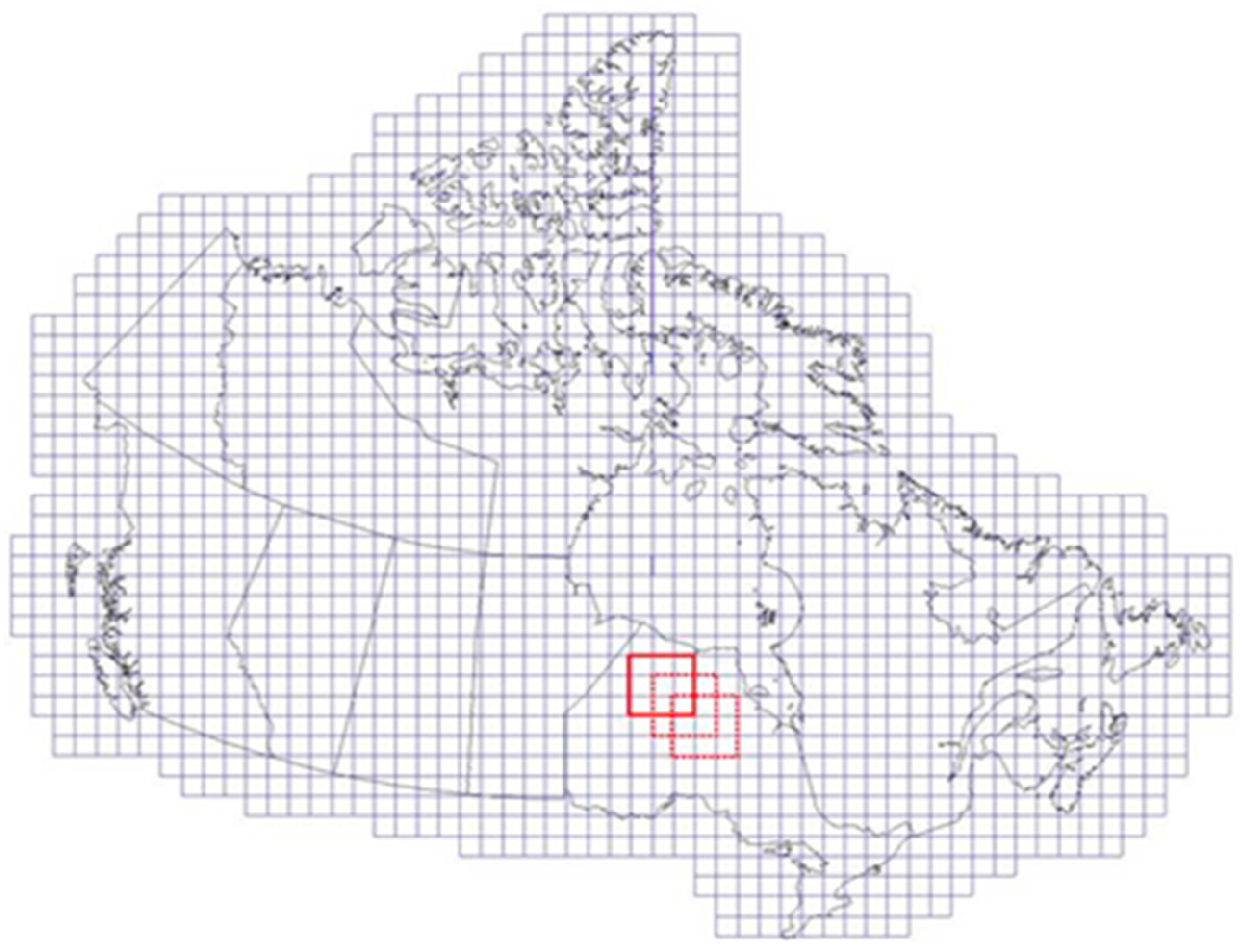
Figure 2 shows the windows configuration used for local classifier optimization and blending. Overall, 1472 windows and corresponding RF models were generated and applied to produce the land cover of Canada. Implementation of the above-described approach might not be feasible on a regular workstation, for there is very high processing demand. Therefore, this study’s methods were developed and deployed on the Government of Canada’s High-Performance Computing Centre (HPC). In parallel processing mode on 1300 cores, processing time was about 2 h.
2.3.3. Mapping of Urban and Agriculture Areas
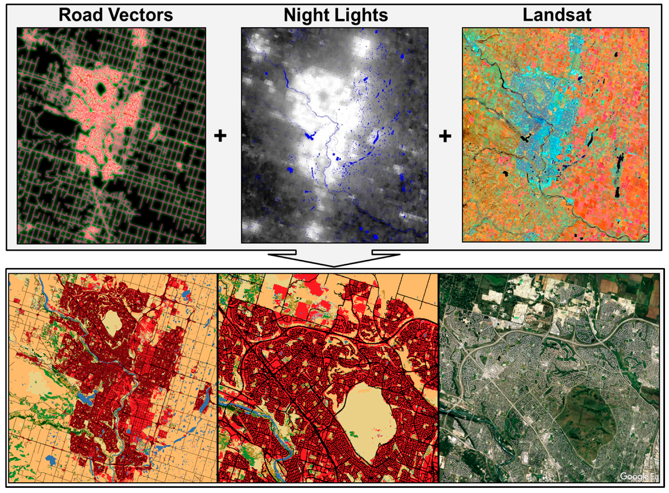
Urban mapping was developed separately. Initially, two density-based classes of industrial and built-up lands were deciphered from road density data at 1 km and 5 km scales, Landsat reflectance and the Nightly Mosaic of the Visible Infrared Imaging Radiometer Suite (VIIRS) data. These were merged to a final urban and built-up class (class 17 in Table 3). For each tile, the two urban classes were sampled and used to train RF with these features as inputs. Figure 3 provides a schematic of the processing applied. Results were generally very good, except in agriculture regions where the Landsat data quality was poor. In these regions, considerable manual correction was undertaken. Roads were also rasterized to 30 m, and added to the map.
Highly dynamic areas such as agricultural regions present a particular challenge, since inter-scene radiometric consistency can be affected by crop rotation and growing practices. The cropland class was also mapped separately, and is based on the existing agriculture crop cover classification dataset (Table 2), which was used to extract samples for training RF models.
2.3.4. Additional Corrections and Quality Control
Several additional processing steps were required to create the final product. In the far north, above 83 degrees latitude, Landsat data is not collected. For this area, land cover from MODIS was used [8]. In addition, in some regions of the north, missing values resulted from a low sun angle and topography. For these areas, a majority filter within a 5 × 5 window was used to estimate missing values. Finally, in mountain regions, strong topographic effects occurred due to shadows. To correct this, a water mask derived from http://geogratis.cgdi.gc.ca and digital elevation data was used to identify shadow-affected areas within the mountain regions. MODIS observations were then used to estimate reflectance by averaging the spectrally closest 50 Landsat values to MODIS. As MODIS uses different sun azimuth angles, it can obtain a non-shadow or reduced shadow observation. If no suitable observations were identified, then the shadow-affected areas were filled with the majority label of unaffected spatial neighbors (Figure 4).
Post classification operations also included additional image processing performed in cases of known confusion. For example, spectrally similar classes such as low biomass, cropland, and grassland were confused with each other, or with tundra. Therefore, a tundra mask was generated for the area north of the tree line, delimited by Timoney et al. [17], and an agriculture mask was produced from a minimum red reflectance winter composite and an integrated summer Normalized Difference Vegetation Index (NDVI) image. These masks were used to separate spectrally similar pixels in the northern treeless and agriculture regions by changing the class labels for the appropriate clusters beneath these masks. The water body areas were corrected using the water mask generated from the National Hydro Network’s 1:50,000 scale data.
3. Results
Figure 5 shows the land cover classification generated using algorithms described in Section 2.3. To achieve the required quality (i.e., accuracy and spatial consistency) over a large area is not a simple, straightforward procedure. Any large-area land cover map constructed from remotely sensed data is limited in the accuracies it can achieve. Challenges include satellite-sensor data limitations, and issues associated with the generalization and abstraction of the real land surface. Most of the land cover types at a large scale comprise a wide range of variation in vegetation species, structure, and understory. In such a high-variance environment, mapping approaches need considerable tuning to achieve consistent accuracy. The mapping approach used in this study includes systematic qualitative examinations of the following map quality characteristics: (1) measure of classification algorithm confidence; (2) land cover spatial distribution consistency; (3) assessment of known regional land cover type confusions; and (4) representation of known local change drivers. Factors 1 and 2 are described in the next sections in further detail. Factors 3 and 4 are listed, as they are generally important considerations for large-area land cover mapping.
4. Discussion
4.1. Classification Algorithm Confidence
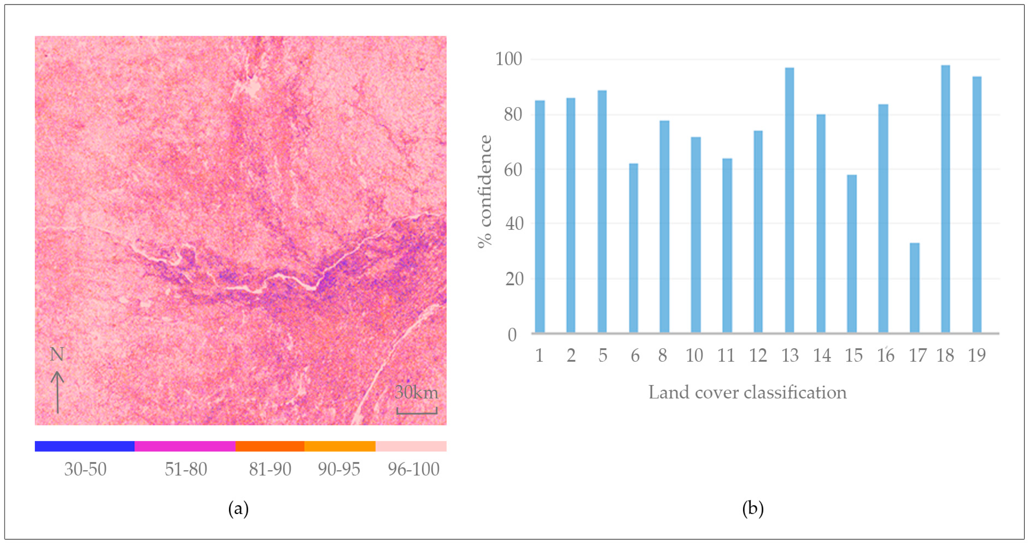
The posterior probability of the assigned label to each pixel is useful information for map confidence-based quality and accuracy assessment [36]. The concept of confidence-based quality assessment was first described in detail in the remote sensing literature by Strahler et al. [37]. In our study, it is based on voting the random forest trees, and it is computed as the proportion of trees that predict a certain label. The posterior probabilities can be used to quantify classification map quality in a spatially explicit fashion (Figure 6a). This measure tends to follow accuracy; however, it is not true accuracy, because if a given pixel is not similar to any of the training data, the classifier will still assign a label and compute the posterior probability. The graph in Figure 6b shows the confidence for each land cover type computed as the average confidence of all the pixels labeled with a given class. Classes 17 and 15, urban (34%) and cropland (57%), showed the lowest confidence and necessitated imposing additional revision of the mapping approach to achieve better classifier confidence. A classifier for urban and cropland mapping was designed and trained separately with additional features, as described in Section 2.3.4. The snow (17), water (18), and sub-polar barren–lichen–moss (13) classes showed the highest mapping confidence (93–97%), which was anticipated considering their easily distinguishable signature. Forest classes (1, 2, 5, and 6) revealed good mapping confidence (85–91%). Other classes were between 75% and 85%, with a somewhat lower mapping confidence of 70% for the sub-polar shrubland–lichen–moss class. Overall, average classification confidence weighted by class area was 87%. The results of the map confidence-based quality analysis did not identify any additional issues.
4.2. Land Cover Spatial Distribution Consistency
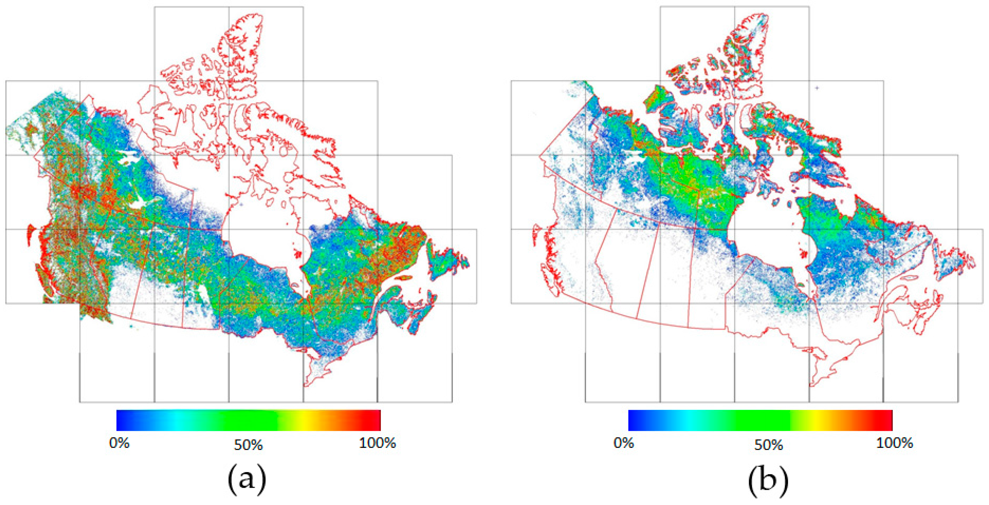
To assess spatial consistency between tiles and the expected cover distribution for a class, the fraction of each class was depicted across Canada in a separate map layer at 300 m spatial resolution, where the pixels’ values represented the percent occupied by the specific land cover class. As an example of these maps, the temperate or sub-polar needle leaf forest fraction is shown in Figure 7a, and the sub-polar or polar grassland–lichen–moss fraction is shown in Figure 7b. Such maps were generated and closely examined for each class. The examination of the fractional maps derived from final land cover data did not reveal any discontinuity between mapping tiles, which confirmed the effectiveness of the local optimization and blending procedures described in Section 2.3.3.
The fractional maps were also used to assess the correctness of the spatial distribution of each land cover class using class-particular characteristics. For example, Figure 6a illustrates the extent of needleleaf forest that generally agrees with the expected class distribution (i.e., absence of the forest above the treeless line, and a very small amount of needleleaf forest in the prairie region). Moreover, such analysis of fractional maps helped in ensuring separation between temporal, sub-polar, and polar classes. Some corrections were required to spatially separate temporal or sub-polar shrubland from sub-polar or polar shrubland–lichen–moss, and temporal grassland from sub-polar or polar grassland classes.
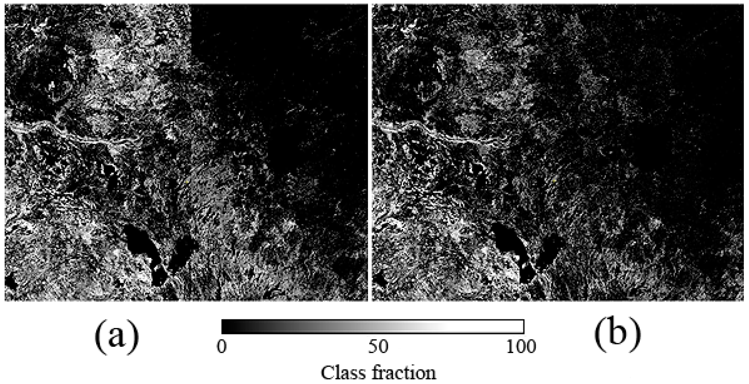
The fraction maps were also useful in highlighting discontinuities between tiles and showing the effect of the window-based local optimization and blending methodology. Figure 8 shows the effect of blending for the mixed forest class. Often, these discontinuities can be missed when examining land cover, as less frequent classes are drowned-out relative to the dominant class in a region.
4.3. Local Classifier Characteristics
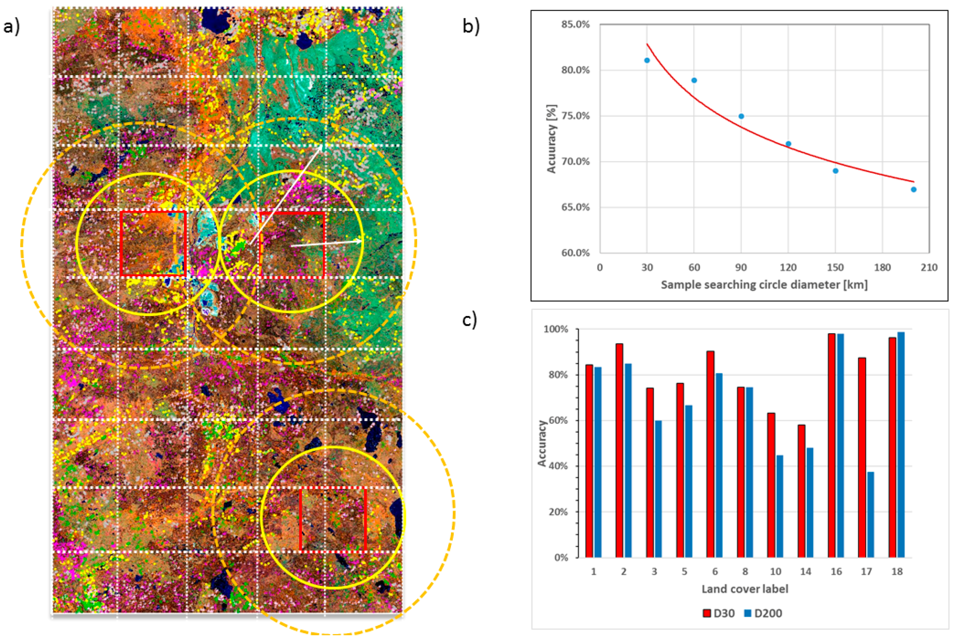
To investigate the effect of the described mapping approach with classifier local optimization on the land cover accuracy, we carried out a detailed analysis over a region in northeast Alberta. The region is 200 km × 350 km in extent, and represents boreal forest with very diverse land cover distribution and a significant amount of disturbance caused by intensive industrial development. An additional reason for selecting this region was the availability of sufficient reference data collected through intensive fieldwork and the availability of very fine resolution images. The training dataset contained 18,500 reference samples (i.e., 0.024% of the mapping area). Independent validation data contained 800 ground truth samples compiled from a number of fieldwork campaigns performed over the 2009–2011 period.
To assess the influence of local sample selection (i.e., signature extension), the diameter of the sample-searching circle was varied from 30 km to 200 km, in 30 km increments. The study area was divided into 112 classification windows of 24 km × 24 km (Figure 9). A local RF model was trained for each classification window using all of the samples inside the corresponding sample-searching circle. Overall, six land cover maps were produced and compared against the validation data set. Figure 9b shows an increase of the overall land cover mapping accuracy with localization of the training sample. The overall mapping accuracy changed from 67% to 81% as a function of the diameter of the sample-searching circle. Figure 9c shows the comparison between the accuracy of land cover maps produced with the model trained with all reference data (i.e., traditional random forest approach) versus that of land cover maps produced with the models trained using only local subsamples. Table 5 presents an evaluation of the statistical significance of the difference [38] between classifications accuracies produced by the traditional random forest approach and the approach using local optimization. The largest gain in accuracy was achieved when mapping land cover classes had smaller areal extents. When land cover classes had larger areal extents, which were mostly uniformly distributed, the gain in accuracy using locally optimized models was smaller. The increase of accuracy for localized classes is understandable, because when the training sample is also localized, there is less probability that classes occurring with greater frequency (i.e., extent) can overwhelm the model, and be assigned to given pixels at the expense of more infrequent but legitimate land cover classes. Another advantage is that the locally optimized RF model is less likely to result in the spectral confusion of classes with similar spectral signatures, but different spatial distribution. Shortcomings of the approach include the need for a large number of samples that are uniformly distributed spatially, and increased processing time.
4.4. Land Cover Map Accuracy Assessment
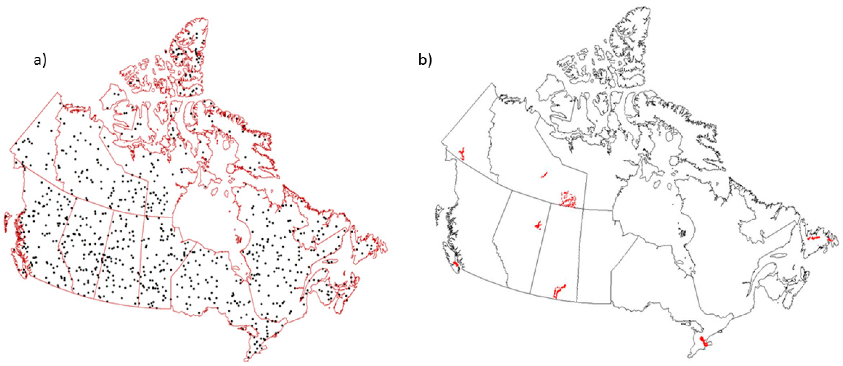
The accuracy of the Land Cover Map of Canada 2010 was assessed against 2811 reference samples (Figure 10) For 839 randomly selected samples (Figure 10a), labels were determined through land cover expert interpretation using Google Earth fine resolution images and a false color composite (R–near-infrared (NIR), G–short-wave infrared (SWIR), B–red band) from Landsat ETM+ acquired in 2010. The rest of the data are ground truth data from six different regions (Figure 10b) acquired during field campaigns linked to various CCRS projects between 2009 and 2011. For each sample, the land cover class was defined based on photos and fieldwork records.
Primary and alternate land cover labels for each reference sample were determined for minimum mapping units (MMU) of both 1 × 1 pixel and 12 × 12 pixels. For any pixel with a mixed land cover composition, an interpreter assigned a label based on the most abundant land cover type present. The assessment includes both land cover maps with 1 × 1 and 12 × 12 MMU. The error matrix in Table 6 summarizes the accuracy assessment results using only primary labels, which were tabulated by combining all of the reference samples from both datasets. It shows that 2180 out of 2811 (77.60%) samples are in agreement with land cover classifications. Commission and omission errors are specified in columns and rows. In order to report accuracy that reflects the overall land cover map, the user’s and producer’s accuracy were weighted by the class area for 1 × 1 and 12 × 12 MMU maps. Table 7 shows the overall average accuracy for two definitions of agreement: (1) an overall accuracy when agreement is defined as a match between the map class and either the primary or alternate reference; and (2) when agreement is defined using only the primary reference label.
The error matrix analysis reveals anticipated sources of spectral confusion among land cover classes. Adjacent forest classes tend to be confused, for example, coniferous with mixed forest, as well as deciduous forest, shrubland, shrub-covered wetlands, and certain croplands. These classes are difficult to separate with spectral data alone, since all are primarily broadleaved deciduous. Radiometric saturation occurs at the leaf area index levels in the range of 3–5 [39], which is typical of all three classes. Confusion also arose with the herbaceous class, which was misidentified as either low biomass croplands, or sparse conifer along the tree line consisting of open treed areas with herbaceous understory. Confusion also occurred between the herbaceous and sub-polar shrub classes due to the relatively small spectral differences between them. Finally, reference data indicated that the lichen–moss class was confused with either the herbaceous or the wetland classes, due to the prevalence of both lichen and moss in certain wetlands, and the low biomass, which characterizes both the lichen–moss and herbaceous classes.
5. Conclusions
A nationally consistent map depicting the distribution of land cover with a high spatial resolution (~30 m) is an urgent requirement for various scientific, policy, and reporting purposes, and has only recently become fully feasible. Based on research carried out at the Canada Centre for Remote Sensing, this paper describes a new methodology that makes optimum use of satellite data to generate a very accurate product while minimizing the costs of a mapping program at the national scale. It relies on expert knowledge for generating initial reference data, which are used to train machine-learning algorithms operating in a high-performance computing environment that essentially enables intensive, fully automated mapping. The innovative features of the new methodology are: classifier local optimization and blending; quantitative confidence assessment based on overlapping areas and posterior probability of the assigned labels; and thoughtful involvement of the analyst at key stages of the quality assessment. Results show that the approach achieved the objective of spatial consistency and reasonable accuracy at approximately 75–80%, depending on the nature of the assessment. However, for some classes, accuracy was considered too low, and needs to be improved.
Acknowledgments
This research was financially supported by the Canadian Space Agency under Government Related Initiatives Program (Grant No. 17MOA41001). The authors would like to thank Calvin Poff for assisting in much of the quality control efforts undertaken in this work.
Author Contributions
Rasim Latifovic wrote the manuscript with contributions from all authors. Rasim Latifovic developed and implemented the software, performed the processing and analyzed the results; Rasim Latifovic and Darren Pouliot conceived and designed the mapping approach; Ian Olthof contributed to reference data processing and analysis.
Conflicts of Interest
The authors declare no conflict of interest.
References
- DB Geoservices Inc. GeoBase Land Cover Products User Needs Assessment; Agriculture and Agri-Food Canada: Ottawa, ON, Canada, 2008.
- GCOS. Systematic Observation Requirements for Satellite-Based Products for Climate Supplemental Details to the Satellite-Based Component of the Implementation Plan for the Global Observing System for Climate in Support of the UNFCCC; World Meteorological Organization (WMO): Geneva, Switzerland, 2006; Available online: https://library.wmo.int/opac/doc_num.php?explnum_id=3710 (accessed on 26 October 2017).
- CEOS. Satellite Observation of the Climate System: The Committee on Earth Observation Satellites (CEOS) Response to the Implementation Plan for the Global Observing System for Climate in Support of the UNFCCC. 2006; p. 54. Available online: ftp://ftp.ncdc.noaa.gov/pub/data/sds/CEOS-Response-to-the-GCOS-IP.pdf (accessed on 26 October 2017).
- Global Terrestrial Observing System (GTOS). Terrestrial Essential Climate Variables. Biennial Report Supplement for Climate Change Assessment, Mitigation and Adaptation. 2008, p. 44. Available online: ftp://ftp.fao.org/docrep/fao/011/i0197e/i0197e.pdf (accessed on 26 October 2017).
- Beaubien, J.; Cihlar, J.; Simard, G.; Latifovic, R. Land Cover from Multiple Thematic Mapper Scenes Using a New Enhancement-Classification Methodology. J. Geophys. Res. Atmos. 1999, 104, 27909–27920. [Google Scholar] [CrossRef]
- Latifovic, R.; Zhu, Z.L.; Josef, C.; Chandra, G.; Ian, O. Land Cover Mapping of North and Central America—Global Land Cover 2000. Remote Sens. Environ. 2004, 89, 116–127. [Google Scholar] [CrossRef]
- Pouliot, D.; Latifovic, R.; Zabcic, N.; Guindon, L.; Olthof, I. Development and Assessment of a 250 m Spatial Resolution MODIS Annual Land Cover Time Series (2000–2011) for the Forest Region of Canada Derived from Change-Based Updating. Remote Sens. Environ. 2014, 140, 731–743. [Google Scholar] [CrossRef]
- Latifovic, R.; Homer, C.; Ressl, R.; Pouliot, D.; Hossain, S.N.; Colditz, R.R.; Olthof, I.; Giri, C.P.; Victoria, A. North American Land Change Monitoring System. Remote Sens. Land Use Land Cover Princ. Appl. 2012, 303–324. [Google Scholar]
- Colditz, R.R.; Pouliot, D.; Llamas, R.M.; Homer, C.; Latifovic, R.; Ressl, R.A.; Tovar, C.M.; Hernandez, A.V.; Richardson, K. Detection of North American Land Cover Change between 2005 and 2010 with 250 m MODIS Data. Photogramm. Eng. Remote Sens. 2014, 7, 3358–3372. [Google Scholar]
- Latifovic, R.; Pouliot, D.A. Multi-Temporal Land Cover Mapping for Canada: Methodology and Products. Can. J. Remote Sens. 2005, 31, 347–363. [Google Scholar] [CrossRef]
- Latifovic, R.; Pouliot, D.; Sun, L.; Schwarz, J.; Parkinson, W. Moderate Resolution Time Series Data Management and Analysis: Automated Large Area Mosaicking and Quality Control; Geomatics Canada. Open File 2015, 6, 25. Available online: https://doi.org/10.4095/296204 (accessed on 26 October 2017).
- National Road Network, 1:50,000 Scale Geogratis. Available online: http://www.nrcan.gc.ca/earth-sciences/geography/topographic-information/free-data-geogratis/whats-new/17213 (accessed on 26 October 2017).
- SILC: Satellite Database for the Land cover of Canada Sample of LANDSAT TM/ETM+ Scenes (30 m Resolution). Available online: ftp://ftp.ccrs.nrcan.gc.ca/ad/silc (accessed on 26 October 2017).
- Wulder, M.A.; Cranny, M.M.; Hall, R.J.; Luther, J.E.; Beaudoin, A.; White, J.C.; Goodenough, D.G.; Dechka, J.A. Satellite Land Cover Mapping of Canada’s Forests: The EOSD Land Cover Project; Campbell, J.C., Jones, K.B., Smith, J.H., Koeppe, M.T., Eds.; North America Land Cover Summit; American Association of Geographers: Washington, DC, USA, 2008; pp. 21–30. Available online: https://cfs.nrcan.gc.ca/publications?id=29220 (accessed on 26 October 2017).
- Olthof, I.; Latifovic, R.; Pouliot, D. Development of a Circa 2000 Land Cover Map of Northern Canada at 30 m Resolution from Landsat. Can. J. Remote Sens. 2009, 35, 152–165. [Google Scholar] [CrossRef]
- Annual Crop Inventory. Available online: http://open.canada.ca/data/en/dataset/ba2645d5-4458-414d-b196-6303ac06c1c9 (accessed on 26 October 2017).
- Timoney, K.P.; Roi, G.H.L.; Zoltai, S.C.; Robinson, A.L. The High Subarctic Forest-Tundra of Northwestern Canada: Position, Width, and Vegetation Gradients in Relation to Climate. ARCTIC 1992, 45, 1–9. [Google Scholar] [CrossRef]
- De Groot, W.J.; Landry, R.; Kurz, W.A.; Anderson, K.R.; Englefield, P.; Fraser, R.H.; Hall, R.J.; Banfield, G.E.; Raymond, D.A.; Decker, V.; et al. Estimating Direct Carbon Emissions from Canadian Wildland Fires. Int. J. Wildland Fire 2007, 16, 593–606. [Google Scholar] [CrossRef]
- National Centers for Environmental Information. Available online: https://www.ncei.noaa.gov/ (accessed on 28 August 2017).
- Breimann, L.; Friedman, J.; Ohlsen, R.; Stone, C. Classification and Regression Trees; Taylor & Francis Group, LLC: Abingdon, UK, 1984. [Google Scholar]
- DeFries, R.; Hansen, M.; Townshend, J.R.G.; Sohlberg, R. Global Land Cover Classifications at 8 km Spatial Resolution: The Use of Training Data Derived from Landsat Imagery in Decision Tree Classifiers. Int. J. Remote Sens. 1998, 19, 3141–3168. [Google Scholar] [CrossRef]
- Hansen, M.; Dubayah, R.; DeFries, R. Classification Trees: An Alternative to Traditional Land Cover Classifiers. Int. J. Remote Sens. 1996, 17, 1075–1081. [Google Scholar] [CrossRef]
- Friedl, M.A.; Brodley, C.E.; Strahler, A. Land Cover Classification Accuracies Produced by Decision Trees at Continental to Global Scales. IEEE Trans. Geosci. Remote Sens. 1999, 37, 969–977. [Google Scholar] [CrossRef]
- Friedl, M.A.; McIver, D.K.; Hodges, J.C.F.; Zhang, X.Y.; Muchoney, D.; Strahler, A.H.; Woodcock, C.E.; Gopal, S.; Schneider, A.; Cooper, A.; et al. Global Land Cover Mapping from MODIS: Algorithms and Early Results. Remote Sens. Environ. 2002, 83, 287–302. [Google Scholar] [CrossRef]
- Friedl, M.A.; Sulla-Menashe, D.; Tan, B.; Schneider, A.; Ramankutty, N.; Sibley, A.; Xiaoman, H. MODIS Collection 5 Global Land Cover: Algorithm Refinements and Characterization of New Datasets. Remote Sens. Environ. 2010, 114, 168–182. [Google Scholar] [CrossRef]
- Gislason, P.O.; Benediktsson, J.A.; Sveinsson, J.R. Pattern Recognition Letters—Special Issue: Pattern Recognit. Remote Sens. Arch. 2006, 27, 294–300. [Google Scholar] [CrossRef]
- Pal, M. Random Forest Classifier for Remote Sensing Classification. Int. J. Remote Sens. 2005, 26, 217–222. [Google Scholar] [CrossRef]
- Rodriguez-Galiano, V.F.; Ghimire, B.; Rogan, J.; Chica-Olmo, M.; Rigol-Sanchez, J.P. An Assessment of the Effectiveness of a Random Forest Classifier for Land-Cover Classification. ISPRS J. Photogramm. Remote Sens. 2012, 67, 93–104. [Google Scholar] [CrossRef]
- Breimann, L. Random Forests. Mach. Learn. 2001, 45, 5–32. [Google Scholar] [CrossRef]
- Chittineni, C.B. Signature extension in remote sensing. Pattern Recognit. 1980, 12, 243–249. [Google Scholar] [CrossRef]
- Fernandes, R.; Fraser, R.; Latifovic, R.; Cihlar, J.; Beaubien, J.; Du, Y. Approaches to Fractional Land Cover and Continuous Field Mapping: A Comparative Assessment over the BOREAS Study Region. Remote Sens. Environ. 2004, 89, 234–251. [Google Scholar] [CrossRef]
- Cihlar, J.; Guindon, B.; Beaubien, J.; Latifovic, R.; Peddle, D.R.; Wulder, M.A.; Fernandes, R.; Kerr, J. From Need to Product: A Methodology for Completing a Land Cover Map of Canada with Landsat Data. Can. J. Remote Sens. 2003, 29, 171–186. [Google Scholar] [CrossRef]
- Homer, C.; Dewitz, J.; Fry, J.; Coan, M.; Hossain, N.; Larson, C.; Herold, N.; McKerrow, A.; VanDriel, J.N.; Wickham, J. Completion of the 2001 National Land Cover Database for the Conterminous United States. Photogramm. Eng. Remote Sens. 2007, 73, 337–341. [Google Scholar]
- Pouliot, D.; Latifovic, R.; Parkinson, W. Influence of Sample Distribution and Prior Probability Adjustment on Land Cover Classification. Geomatics Canada, Open File 23, 2016, 13 pages. Available online: http://ftp.maps.canada.ca/pub/nrcan_rncan/publications/ess_sst/297/297517/of_0023_gc.pdf (accessed on 26 October 2017).
- Millard, K.; Richardson, M. On the Importance of Training Data Sample Selection in Random Forest Image Classification: A Case Study in Peatland Ecosystem Mapping. Remote Sens. 2015, 7, 8489–8515. [Google Scholar] [CrossRef]
- Strahler, A.H.; Boschetti, L.; Foody, G.M.; Friedl, M.A.; Hansen, M.C.; Herold, M.; Mayaux, P.; Morisette, J.T.; Stehman, S.V.; Woodcock, C.E. Global Land Cover Validation: Recommendations for Evaluation and Accuracy Assessment of Global Land Cover Maps; Report of Institute of Environmental Sustainability Global Land Analysis & Discovery (GLAD): College Park, MD, USA, 2006; Available online: http://nofc.cfs.nrcan.gc.ca/gofc-gold/Report%20Series/GOLD_25.pdf (accessed on 26 October 2017).
- Foody, G.; Campbell, N.; Trodd, N.; Wood, T. Derivation and Applications of Probabilistic Measures of Class Membership from the Maximum-Likelihood Classification. Photogramm. Eng. Remote Sens. 1992, 58, 1335–1341. [Google Scholar]
- Foody, G.M. Thematic Map Comparison: Evaluating the Statistical Significance of Differences in Classification Accuracy. Photogramm. Eng. Remote Sens. 2004, 70, 627–633. [Google Scholar] [CrossRef]
- Turner, D.P.; Cohen, W.B.; Kennedy, R.E.; Fassnacht, K.S.; Briggs, J.M. Relationships between Leaf Area Index and Landsat TM Spectral Vegetation Indices across Three Temperate Zone Sites. Remote Sens. Environ. 1999, 70, 52–68. [Google Scholar] [CrossRef]
Figure 1.
Landsat Mosaic of Canada 2010 false color composite Top of Atmosphere reflectance and tile system used for Landsat processing and land cover mapping.
Figure 1.
Landsat Mosaic of Canada 2010 false color composite Top of Atmosphere reflectance and tile system used for Landsat processing and land cover mapping.
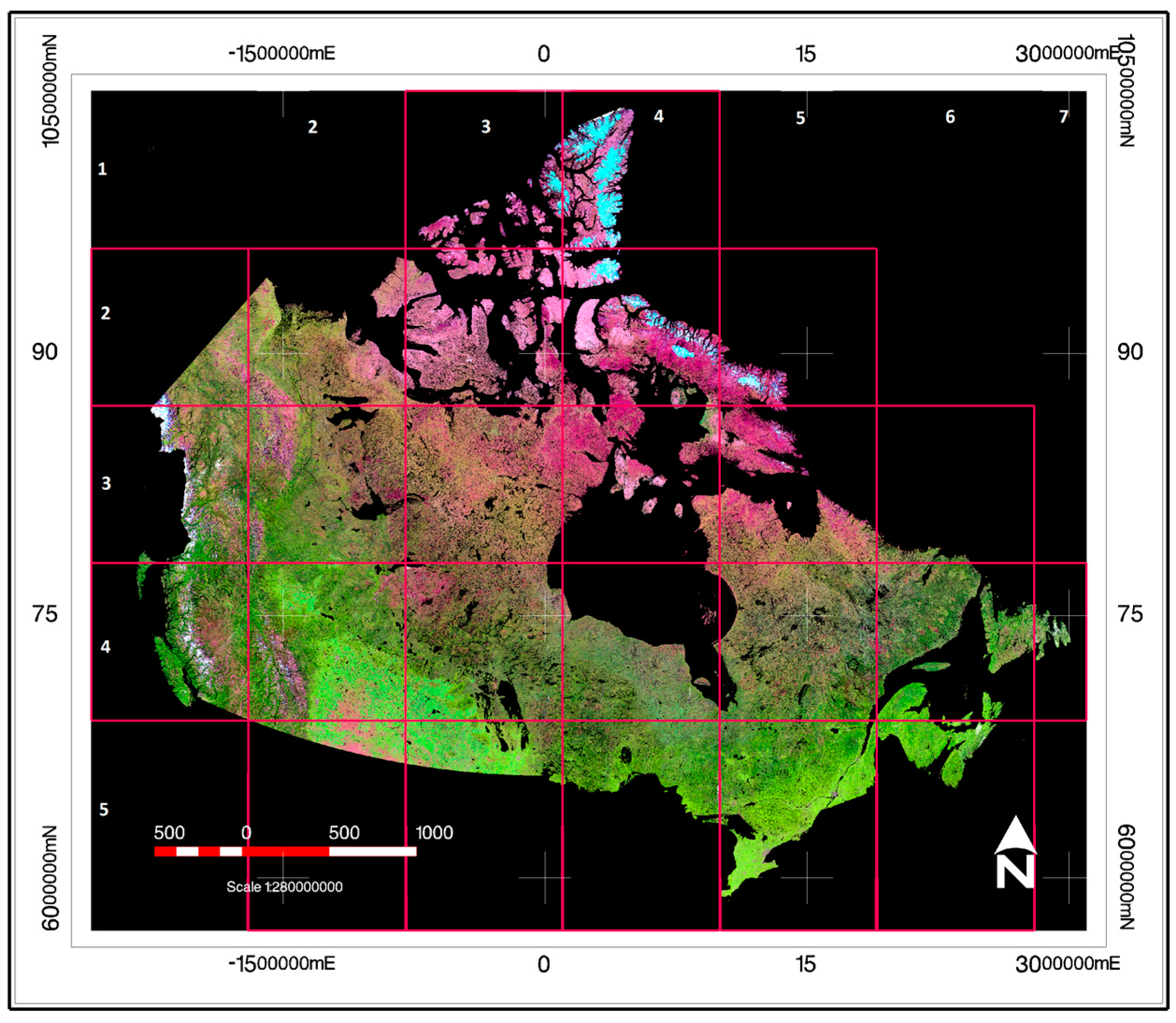
Figure 2.
Configuration of the local optimization windows.

Figure 3.
Approach used for mapping urban and built-up areas. True color image is from Google Earth for 2015.
Figure 3.
Approach used for mapping urban and built-up areas. True color image is from Google Earth for 2015.

Figure 4.
Results of shadow correction in mountain regions, before correction (a) and after (b).
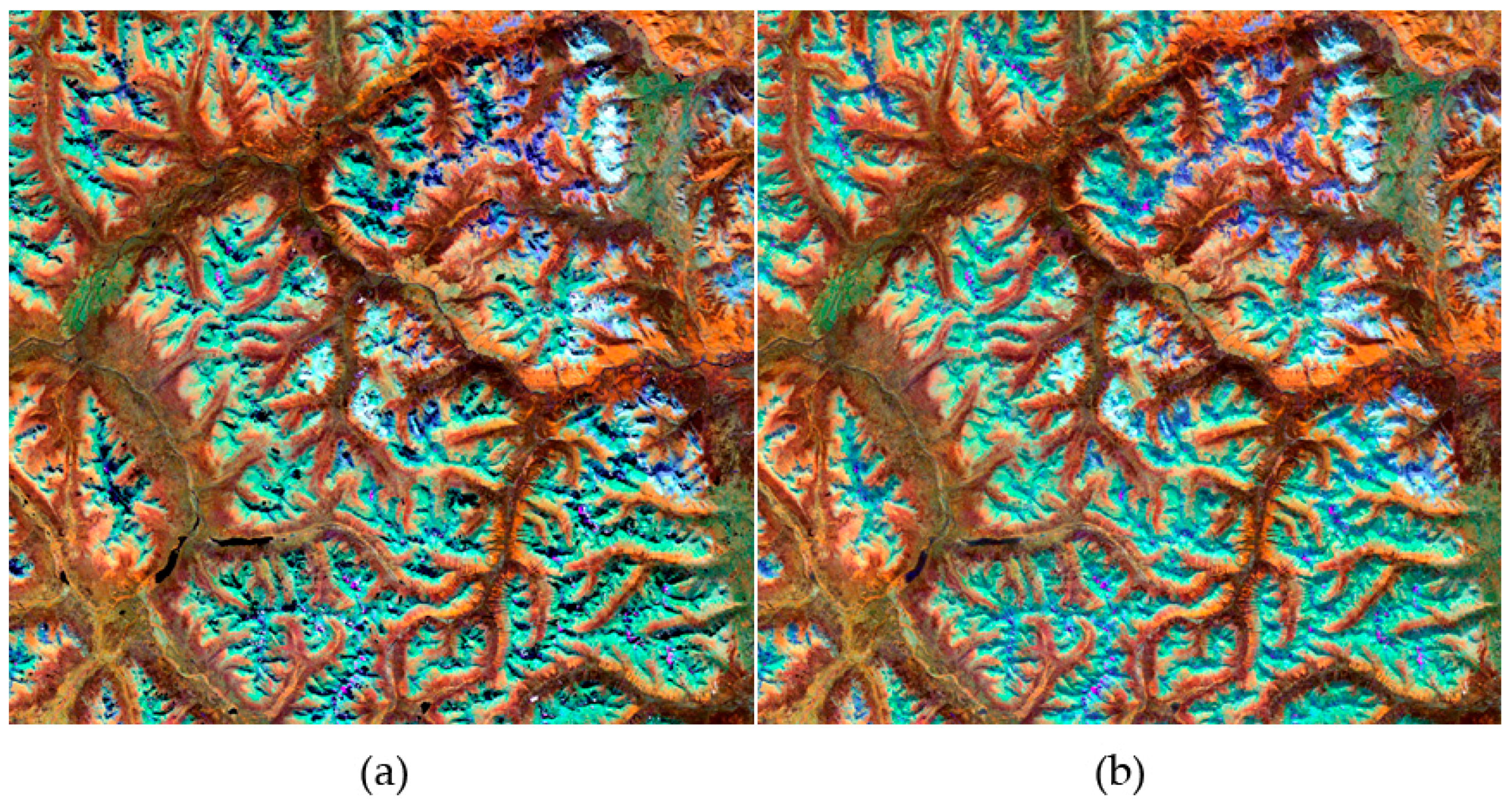
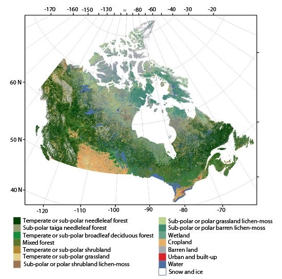
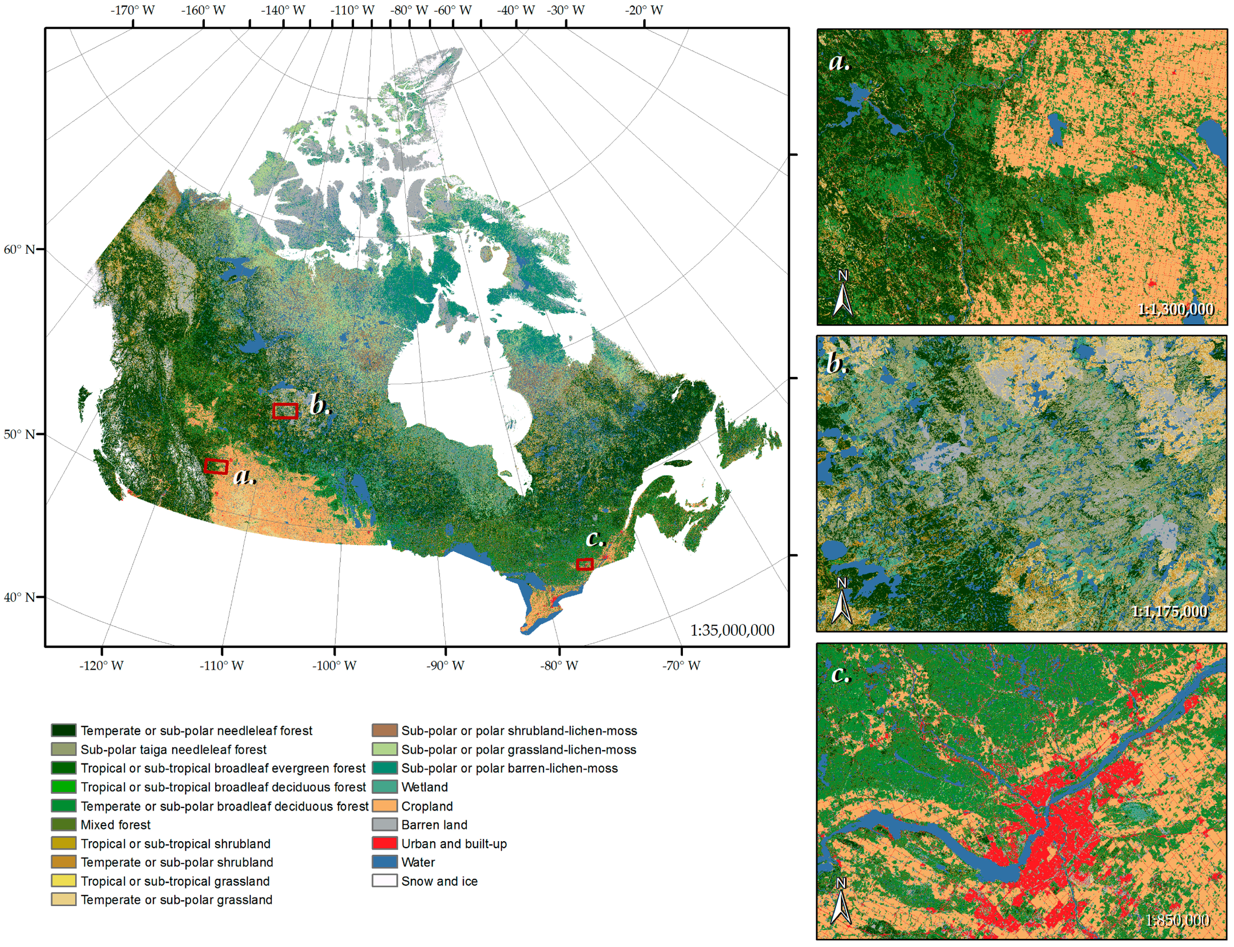
Figure 5.
Land cover of Canada at 30 m spatial resolution for 2010.

Figure 6.
(a) Example of classifier confidence i.e., posterior probability based on voting the random forest trees; (b) average confidence by land cover type.
Figure 6.
(a) Example of classifier confidence i.e., posterior probability based on voting the random forest trees; (b) average confidence by land cover type.

Figure 7.
Fractional maps: (a) Temperate or sub-polar needleleaf forest; (b) Sub-polar or polar grassland–lichen–moss.
Figure 7.
Fractional maps: (a) Temperate or sub-polar needleleaf forest; (b) Sub-polar or polar grassland–lichen–moss.

Figure 8.
The effect of the window-based local optimization on the mixed forest class across tile boundary 4-2 to 4-3, before (a) and after (b).
Figure 8.
The effect of the window-based local optimization on the mixed forest class across tile boundary 4-2 to 4-3, before (a) and after (b).

Figure 9.
Results of the land cover classification accuracy produced by the local classifier optimization. The red squares in image (a) are the areas classified using a local model. Each local model is trained using the sample found inside the sample-search circle. Circles of different circumference are shown around each area being classified. Land cover mapping accuracy as a function of the size of the searching-samples circle is presented in graph (b). Land cover mapping accuracy for two boundary cases are presented in graph (c).

Figure 10.
Spatial distribution of the reference samples used in accuracy assessment (a) obtained from fine resolution data interpretation; and (b) acquired during field work ground truth.
Figure 10.
Spatial distribution of the reference samples used in accuracy assessment (a) obtained from fine resolution data interpretation; and (b) acquired during field work ground truth.


Table 1.
The parameters of the Lambert Conformal Conic (LCC) projection and earth ellipsoid model used for output imagery over Canada.
Table 1.
The parameters of the Lambert Conformal Conic (LCC) projection and earth ellipsoid model used for output imagery over Canada.
| Parameter | Value |
|---|---|
| Earth ellipsoid | GRS 1980 |
| Major semi-axis, a | 6,378,137 (m) |
| First eccentricity | 0.00669438002290 |
| Ellipsoid flattening, f | 0.00335281068118 |
| Projection | LCC |
| 1st parallel | 49.00 (degree) |
| 2nd parallel | 77.00 (degree) |
| Central meridian | −95.00 (degree) |
| Upper left corner | (−2,600,000.0 E (m); 10,500,000.0 N (m)) |
| Lower right corner | (3,100,000.0 E (m); 5,700,000.0 N (m)) |
| Easting | 0 |
| Northing | 0 |
Table 2.
Ancillary data used as aid for generating classifier-training data.
| Title | Source |
|---|---|
| National Hydro Network, 1:50,000 scale | Canada Centre for Mapping and Earth Observation (2004) http://geogratis.gc.ca [12] |
| Canadian Digital Elevation Data, 1:50,000 scale | Canada Centre for Mapping and Earth Observation (2000) http://geogratis.gc.ca [12] |
| National Road Network, 1:50,000 scale | Canada Centre for Mapping and Earth Observation (2012) [12] http://geogratis.gc.ca |
| SILC: Satellite Information for Land Cover of Canada—a sample of LANDSAT Thematic Mapper/Enhanced Thematic Mapper (TM/ETM+) scenes (30 m resolution) | Canada Centre for Mapping and Earth Observation [13] |
| EOSD: Earth Observation for Sustainable Development of Forests Land Cover Classification, circa 2000 at 30 m resolution | Canadian Forest Service http://cfs.nrcan.gc.ca/publications?id = 29220 [14] |
| NLLC: Circa 2000 Northern Land Cover of Canada at 30 m spatial resolution | Canada Centre for Mapping and Earth Observation http://geogratis.cgdi.gc.ca [15] |
| ACCC: Agricultural Crop Cover Classification annual crop inventory, 2013, 30 m spatial resolution | AAFC Science and Technology Branch, Earth Observation Team. http://open.canada.ca [16] |
| Northern treeline | http://data.arcticatlas.org, [17] |
| National Burned Area Composites 2004–2013 | Canadian Forest Service [18] |
| Version 1 Visible Infrared Imaging Radiometer Suite (VIIRS) Day/Night Band Nighttime Lights (2012) | Earth Observation Group, NOAA National Geophysical Data Center [19] |
| Ground truth datasets | NRCan, CCRS, unpublished |
Table 3.
North American Land Change Monitoring System (NALCMS) land cover classification legend level I and II.
Table 3.
North American Land Change Monitoring System (NALCMS) land cover classification legend level I and II.
| Level I | Level II | Land Cover Classification System (LCCS) Basic Classifier | ||
|---|---|---|---|---|
| Primarily vegetated areas | Natural and semi-natural terrestrial and aquatic | 1. Needleleaf forest | 1. Temperate or sub-polar needleleaf forest | A3.A10.B2.XX.D2.E1 |
| 2. Sub-polar taiga needleleaf forest | A3.A10.B2.XX.D1.E2 | |||
| 2. Broadleaf forest | 3. Tropical or sub-tropical broadleaf evergreen forest | A3.A10.B2.XX.D1.E1 | ||
| 4. Tropical or sub-tropical broadleaf deciduous forest | A3.A11.B2.XX.D1.E1 | |||
| 5. Temperate or sub-polar broadleaf deciduous forest | A3.A14.B2.XX.D1.E1 | |||
| 3. Mixed forest | 6. Mixed forest | A3.A10.B2.XX.D2.E1/A3.A10.B2.XX.D1.E2 | ||
| 4. Shrubland | 7. Tropical or sub-tropical shrubland | A4.A20.B3–B9 | ||
| 8. Temperate or sub-polar shrubland | A4.A20.B3–B10 | |||
| 5. Grassland | 9. Tropical or sub-tropical grassland | A6.A20.B4 | ||
| 10. Temperate or sub-polar shrubland | A2.A20.B4.XX.E5 | |||
| 6. Lichen/moss | 11. Sub-polar or polar shrubland–lichen–moss | A4.A11.B3–B10/A2.A20.B4–B12/A8.A11–A13 | ||
| 12. Sub-polar or polar grassland–lichen–moss | A4.A20.B4–B12/A4.A11.B3–B10/A8.A11–A13 | |||
| 13. Sub-polar or polar barren–lichen–moss | A8.A20–A.13/A4.A11.B3–B10/A2.A20.B4–B12 | |||
| 7. Wetland | 14. Wetland | A2.A20.B4.C3 | ||
| Cultivated/managed terrestrial/aquatic | 8. Cropland | 15. Cropland | A4–S1 | |
| Primarily non-vegetated areas | Terrestrial | 9. Barren land | 16. Barren land | A1/A2 |
| 10. Urban and built-up | 17. Urban and built-up | A4 | ||
| Aquatic | 11. Water | 18. Water | A1 | |
| 12. Snow and ice | 19. Snow and ice | A2/A3 | ||
Table 4.
Example of class weighting and label selection from windows.
| Window | 1 | 2 | 3 | 4 | 5 | 6 | 7 | 8 | 9 |
|---|---|---|---|---|---|---|---|---|---|
| Class | Conifer | Conifer | Conifer | Water | Mixed | Mixed | Shrub | Water | Mixed |
| Distance (pixels) | 250 | 3500 | 5000 | 13,000 | 5000 | 9500 | 9400 | 7500 | 1000 |
| Weight | 0.94 | 0.819 | 0.70 | 0.074 | 0.706 | 0.263 | 0.271 | 0.454 | 0.929 |
| Conifer count = 3, summed distance = 2.47 Mixed count = 3, summed distance = 1.90 | |||||||||
Table 5.
Summary of evaluation of the statistical difference between the accuracies of classifications produced by traditional random forest (RF) and local optimization approach.
Table 5.
Summary of evaluation of the statistical difference between the accuracies of classifications produced by traditional random forest (RF) and local optimization approach.
| Comparison of Kappa Coefficients | Comparison of Proportions | |||||||||
|---|---|---|---|---|---|---|---|---|---|---|
| Class. 1 | Class. 2 | k1 | k2 | k1−k2 | Significant? | x1/n1 | x2/n2 | x1/n1−x2/n2 | |z| | Significant? |
| RF | Local RF | 0.63 | 0.78 | −0.155 | Yes, 0.1% | 0.67 | 0.82 | −0.141 | 10.9 | Yes, 0.1% |
Table 6.
Error matrix for the Land Cover Map of Canada 2010 with agreement defined as a match between the map label and the primary reference label. Rows of the error matrix are the map classes, and columns are the reference classes.
Table 6.
Error matrix for the Land Cover Map of Canada 2010 with agreement defined as a match between the map label and the primary reference label. Rows of the error matrix are the map classes, and columns are the reference classes.
| Predicted vs. Reference | Reference | |||||||||||||||||
|---|---|---|---|---|---|---|---|---|---|---|---|---|---|---|---|---|---|---|
| Class | 1 | 2 | 5 | 6 | 8 | 10 | 11 | 12 | 13 | 14 | 15 | 16 | 17 | 18 | 19 | User’s Accuracy | ||
| 1. Temperate or sub-polar needleleaf forest | 381 | 1 | 10 | 27 | 21 | 4 | 0 | 0 | 0 | 18 | 0 | 5 | 0 | 1 | 0 | 381 | 468 | 81.4 |
| 2. Sub-polar taiga needleleaf forest | 7 | 13 | 0 | 0 | 1 | 2 | 1 | 0 | 0 | 4 | 0 | 0 | 0 | 0 | 0 | 13 | 28 | 46.4 |
| 5. Temperate or sub-polar broadleaf forest | 14 | 2 | 117 | 13 | 24 | 6 | 3 | 1 | 0 | 2 | 4 | 2 | 2 | 0 | 0 | 117 | 190 | 61.6 |
| 6. Mixed forest | 33 | 0 | 15 | 88 | 15 | 1 | 0 | 0 | 0 | 0 | 0 | 1 | 1 | 1 | 0 | 88 | 155 | 56.8 |
| 8. Temperate or sub-polar shrubland | 15 | 3 | 5 | 6 | 154 | 13 | 22 | 0 | 0 | 7 | 5 | 6 | 0 | 0 | 0 | 154 | 236 | 65.3 |
| 10. Temperate or sub-polar grassland | 5 | 2 | 1 | 1 | 17 | 92 | 0 | 2 | 1 | 1 | 6 | 23 | 0 | 0 | 0 | 92 | 151 | 60.9 |
| 11. Sub-polar or polar shrubland-lichen-moss | 0 | 0 | 0 | 0 | 8 | 0 | 29 | 0 | 0 | 0 | 0 | 0 | 0 | 0 | 0 | 29 | 37 | 78.4 |
| 12. Sub-polar or polar grassland-lichen-mod | 2 | 0 | 0 | 1 | 1 | 1 | 1 | 33 | 0 | 0 | 0 | 4 | 0 | 1 | 0 | 33 | 44 | 75.0 |
| 13. Sub-polar or polar barren-lichen-moss | 0 | 0 | 0 | 0 | 0 | 0 | 0 | 0 | 13 | 6 | 0 | 6 | 0 | 0 | 1 | 13 | 26 | 50.0 |
| 14. Wetland | 6 | 0 | 2 | 3 | 8 | 5 | 1 | 2 | 1 | 67 | 0 | 2 | 0 | 1 | 0 | 67 | 98 | 68.4 |
| 15. Cropland | 5 | 0 | 18 | 2 | 23 | 49 | 0 | 0 | 0 | 4 | 735 | 0 | 3 | 0 | 0 | 735 | 839 | 87.6 |
| 16. Barren land | 2 | 1 | 0 | 2 | 1 | 5 | 1 | 0 | 1 | 0 | 5 | 86 | 1 | 1 | 6 | 86 | 112 | 76.8 |
| 17. Urban | 2 | 0 | 6 | 0 | 5 | 6 | 0 | 0 | 0 | 0 | 8 | 5 | 124 | 0 | 0 | 124 | 156 | 79.5 |
| 18. Water | 1 | 0 | 1 | 0 | 3 | 0 | 2 | 0 | 0 | 5 | 1 | 1 | 0 | 210 | 0 | 210 | 224 | 93.8 |
| 19. Snow and ice | 0 | 0 | 0 | 0 | 0 | 0 | 0 | 0 | 0 | 0 | 0 | 9 | 0 | 0 | 38 | 38 | 47 | 80.9 |
| number of samples | 473 | 22 | 175 | 143 | 281 | 184 | 60 | 38 | 16 | 114 | 764 | 150 | 131 | 215 | 45 | 2180 | ||
| Producer’s Accuracy | 80.5 | 59.1 | 66.9 | 61.5 | 54.8 | 50.0 | 48.3 | 86.8 | 81.3 | 58.8 | 96.2 | 57.3 | 94.7 | 97.7 | 84.4 | Overall | 2811 | 77.6 |
Table 7.
Average accuracy for the land cover maps with 1 × 1 and 12 × 12 minimum mapping units (MMU).
Table 7.
Average accuracy for the land cover maps with 1 × 1 and 12 × 12 minimum mapping units (MMU).
| First Call Only | User’s | Producer’s |
| 1 × 1 MMU pixel count | 74.84 | 73.88 |
| 12 × 12 MMU pixel count | 76.12 | 74.70 |
| First and Second Call | User’s | Producer’s |
| 1 × 1 MMU pixel count | 85.96 | 84.15 |
| 12 × 12 MMU pixel count | 86.05 | 84.33 |
© 2017 by the authors. Licensee MDPI, Basel, Switzerland. This article is an open access article distributed under the terms and conditions of the Creative Commons Attribution (CC BY) license (http://creativecommons.org/licenses/by/4.0/).
Share and Cite
MDPI and ACS Style
Latifovic, R.; Pouliot, D.; Olthof, I. Circa 2010 Land Cover of Canada: Local Optimization Methodology and Product Development. Remote Sens. 2017, 9, 1098. https://doi.org/10.3390/rs9111098
AMA Style
Latifovic R, Pouliot D, Olthof I. Circa 2010 Land Cover of Canada: Local Optimization Methodology and Product Development. Remote Sensing. 2017; 9(11):1098. https://doi.org/10.3390/rs9111098
Chicago/Turabian StyleLatifovic, Rasim, Darren Pouliot, and Ian Olthof. 2017. "Circa 2010 Land Cover of Canada: Local Optimization Methodology and Product Development" Remote Sensing 9, no. 11: 1098. https://doi.org/10.3390/rs9111098
Note that from the first issue of 2016, this journal uses article numbers instead of page numbers. See further details here.