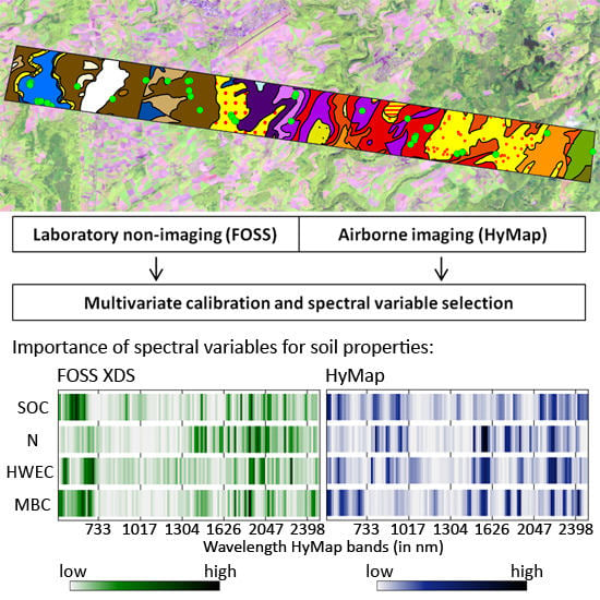
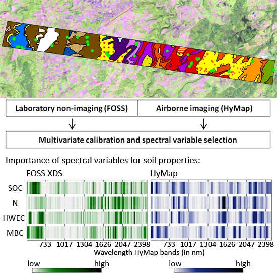
Quantification of Soil Properties with Hyperspectral Data: Selecting Spectral Variables with Different Methods to Improve Accuracies and Analyze Prediction Mechanisms

Abstract

We explored the potentials of both non-imaging laboratory and airborne imaging spectroscopy to assess arable soil quality indicators. We focused on microbial biomass-C (MBC) and hot water-extractable C (HWEC), complemented by organic carbon (OC) and nitrogen (N) as well-studied spectrally active parameters. The aggregation of different spectral variable selection strategies was used to analyze benefits for reachable estimation accuracies and to explore spectral predictive mechanisms for MBC and HWEC. With selected variables, quantification accuracies improved markedly for MBC (laboratory: RPD = 2.32 instead of 1.33 with full spectra; airborne: 2.35 instead of 1.80) and OC (laboratory: RPD = 3.08 instead of 2.36; airborne: 2.20 instead of 1.94). Patterns of selected variables indicated similarities between HWEC and OC, but significant differences between all other soil variables. This agreed to our results of indirect approaches in which both (i) wet-chemical data of OC and N and (ii) spectra fitted to measured OC and N values were used to estimate MBC and HWEC. Compared to these approaches, we found marked benefits of laboratory and airborne data for a direct spectral quantification of MBC (but not for HWEC). This suggests specificity of spectra for MBC, usable for the determination of this important soil parameter.

1. Introduction

Compared to laboratory reflectance spectroscopy in the Vis-NIR-SWIR domain (i.e., in the spectral region between 400 and 2500 nm) with prepared soil samples and well-defined illumination and viewing conditions, the use of imaging spectroscopy (IS) with air- or spaceborne data is far less common for soil applications. One main reason for the limited number of studies with IS is the still restricted data availability. Beyond this, IS approaches suffer from a series of limitations compared to laboratory or also field spectroscopy. To retrieve surface reflectances from the measured radiances, they have to be corrected for atmospheric effects. The signal-to-noise ratio of air- or spaceborne hyperspectral data is relatively low compared to laboratory data due to a low integration time over the target area. Furthermore, a precise georectification of the data is necessary for a correct attribution of collected and analyzed soil samples to image pixels [1,2].

IS is able to measure the reflectance of only the first few millimeters of the soil surface. Variable surface properties affect the spectral assessment of soil properties, as they may blur—depending on the studied target variable—the specific spectral responses that are relevant for calibrating the estimation model. These properties that are subject to variation in space (and also time) are humidity, soil roughness, degree of soil crusting, texture, and the spectral mixture of bare soil with other materials such as vegetation or crop residues. Compared to airborne data, Hyperion satellite hyperspectral data are additionally limited by a lower spatial resolution with a nominal pixel size of 30 m, which increases, for example, the problem of different surfaces mixed in one pixel [1,3,4].

Available studies on the use of airborne hyperspectral (Vis-NIR-SWIR) remote sensing data focus on soil chemical and physical properties including associated soil functions. Estimates were retrieved from image data for soil organic carbon (OC) [5,6,7,8,9], total nitrogen (N) [7], clay, sand or silt content, iron, calcium carbonate, cation exchange capacity, sum of bases, pH, contents of Ca, Mg, K, P and Al [3,5,7,8,10], soil moisture and soil salinity [11]. However, biological soil properties were not in the focus of these studies, although a series of studies exist which use laboratory spectroscopy in the Vis-NIR-SWIR domain for a quantitative assessment of biological soil properties such as microbial biomass-C (MBC) [12,13,14,15,16], microbial biomass-N [15] or soil respiration [12,15].

MBC is a measure of the mass of the living component of soil organic matter. It underpins any biologically related property of soil systems and is essentially linked to nutrient cycles, humification, physical structure formation, degradation of contaminants and soil fertility [17,18]. Thus, MBC and its species and functional diversity are recently gaining significance as bioindicators of soil quality [18,19,20], leading to a huge output of studies throughout the last decade [17,21]. Compared to total OC, MBC is substantially more dynamic and quickly responds to agricultural management changes such as tillage practice, organic amendments and incorporation of cover crops, or to soil moisture and temperature changes. MBC depends on the amount of available soil C substrate, so that the MBC-to-OC ratio indicates the substrate availability to soil microorganisms [22,23,24,25,26]. Nevertheless, MBC and OC may be highly correlated, since Jenkinson and Ladd [27], for example, reported that situations that promote the accumulation of organic matter in general also increase MBC.

For its value as biological soil quality indicator we examined MBC in addition to OC and N. As another indicator of soil quality we also included hot water-extractable C (HWEC), as this fraction can be used to quantify a labile, decomposable part (Cdec, active pool) of OC that is distinguishable from a passive, inert pool of OC. For long-term “steady state”-conditions, the relationship between HWEC and Cdec can be expressed as a constant ratio [22,28]. HWEC sensitively reflects changes in soil organic matter, for example those caused by input, quality and degradation of primary organic material and soil management practices [29,30,31]. However, one has to keep in mind that some studies do question the usefulness of water extractions for an understanding of C dynamics [32].

All four soil variables were tested for whether they could be quantified from laboratory spectroscopic and/or airborne hyperspectral data. However, for MBC and HWEC we hypothesize a spectral assessment that is at least in part linked to that of OC. We refer, for example, to the early study of Chang et al. [12], who attributed good predictions of soil biological properties to spectral responses being very similar to that of soil OC. In contrast, Zornoza et al. [16] found specific wavelength ranges different from those for OC to be most useful for the calibration of MBC (and other microbiological soil properties) from Vis-NIR-SWIR spectra.

Hyperspectral data provide large sets of usually strongly collinear predictor variables, something that is, independent from the target variable, a drawback for a successful calibration. To partly compensate these effects, reduction of dimensionality is a standard approach. Partial least squares regression (PLSR), for example, projects the spectral data into a low-dimensional space formed by a set of orthogonal latent variables with the aim to maximize the covariance between predictors and target variable(s). Currently, PLSR is the most common multivariate calibration method [33], although other approaches have also been applied successfully (see overviews in Viscarra Rossel et al. [34], Vohland et al. [35], Bellino et al. [36]). Furthermore, it has been shown in many studies that it is beneficial to include methods of spectral variable selection in the multivariate modeling process to exclude uninformative spectral variables [37]. The possible benefits are increased estimation accuracies and more parsimonious and thus robust calibration models, which may improve the predictive ability for independent validation samples. Additionally, the selections of informative or key variables can be used to obtain insight in the underlying spectral predictive mechanisms [37,38,39]. However, we have to be aware that relevant mechanisms, e.g., for variables of soil organic matter, may vary from one soil population to another, each with a specific combination of spectrally meaningful factors such as soil texture or color [40,41]. For example, a series of studies (see overview in Cécillon et al. [1]) indicates that only spectral variables being greater than 1100 nm are closely associated with OC, whereas Viscarra Rossel et al. [42] showed that soil color can be used as proxy for an indirect quantification of OC.

Several approaches exist for the selection of an optimal subset of spectral wavelengths (see e.g., overview in Xiaobo et al. [37]), which may be subdivided into different categories, depending on the statistical features of the variables used for selection (such as, for example, regression coefficients or t-statistics) and the way the interaction of variables in the search space is considered, if at all. In general, approaches have to compromise between an exhaustive search through the possible combinations of variables and computational efficiency [39]. Selections will not fully match but differ from one approach to another due to differences in the search procedure. We assume that multi-method selections, and their comparison and synopsis will be worthwhile for deepening an understanding of the specific spectral responses of the studied soil variables. Moreover, they will prove helpful in the analysis—based on similarities and discrepancies between the specific selection patterns—as to what extent predictive mechanisms for the different soil properties are related to each other.

Against this background, the objectives of our study were: (i) to study and compare the usability of laboratory (non-imaging) and airborne (imaging) spectroscopic measurements to estimate OC, N, MBC and HWEC; (ii) to explore whether estimation accuracies increase by the application of different spectral variable selection techniques (in combination with PLSR); (iii) to analyze and compare predictive mechanisms based on the multi-method spectral selection patterns that we obtained for each soil property; and (iv) to clarify whether the quantification of MBC and/or HWEC is based on specific impacts on the spectra or is rather triggered by the relation to the spectrally active constituents OC and N.

Our dataset comprised spectra acquired airborne with the HyMap sensor (Integrated Spectronics, Baulkham Hills, Australia) and measured in the laboratory with a FOSS XDS Rapid Content Analyzer spectrometer (FOSS NIRSystems, Laurel, MD, USA). In total, 42 agricultural plots were sampled during the HyEurope 2009 campaign. Although limited in size, the studied sample set covered a wide range of geological substrates, pH values, soil types and soil texture classes. For the multivariate modeling, we combined PLSR with three different methods of spectral variable selection that implement basically different search strategies for finding the optimal spectral variable subset—“competitive adaptive reweighted sampling” (CARS [43]), a method that “iteratively retains informative variables” (IRIV [39]) and a genetic algorithm (GA [44]).

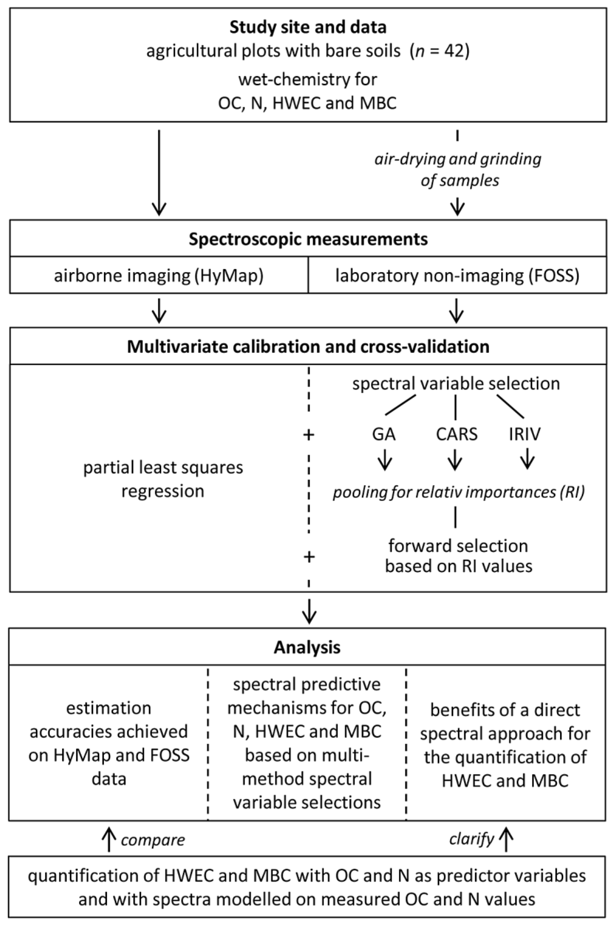
2. Materials and Methods

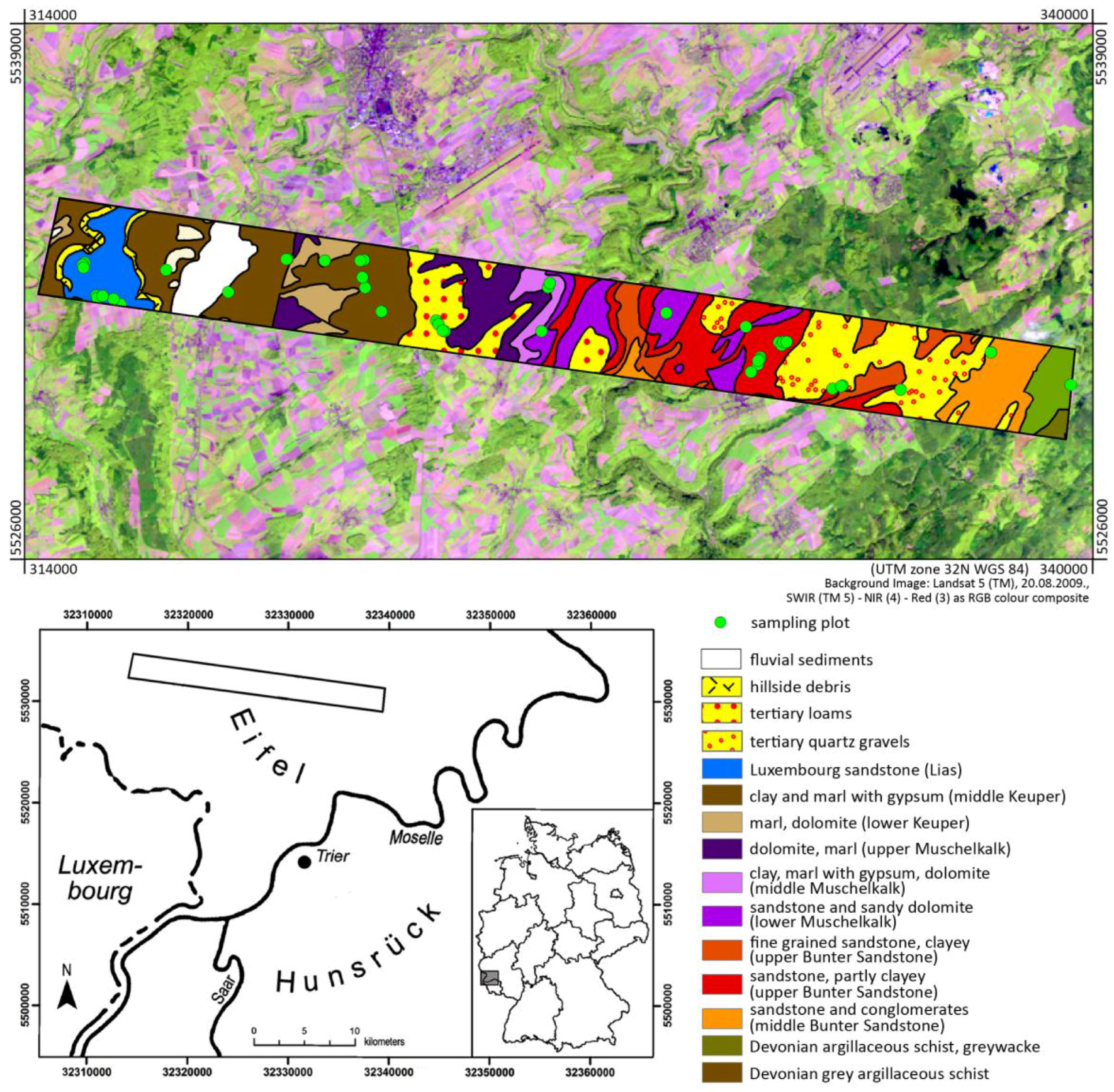
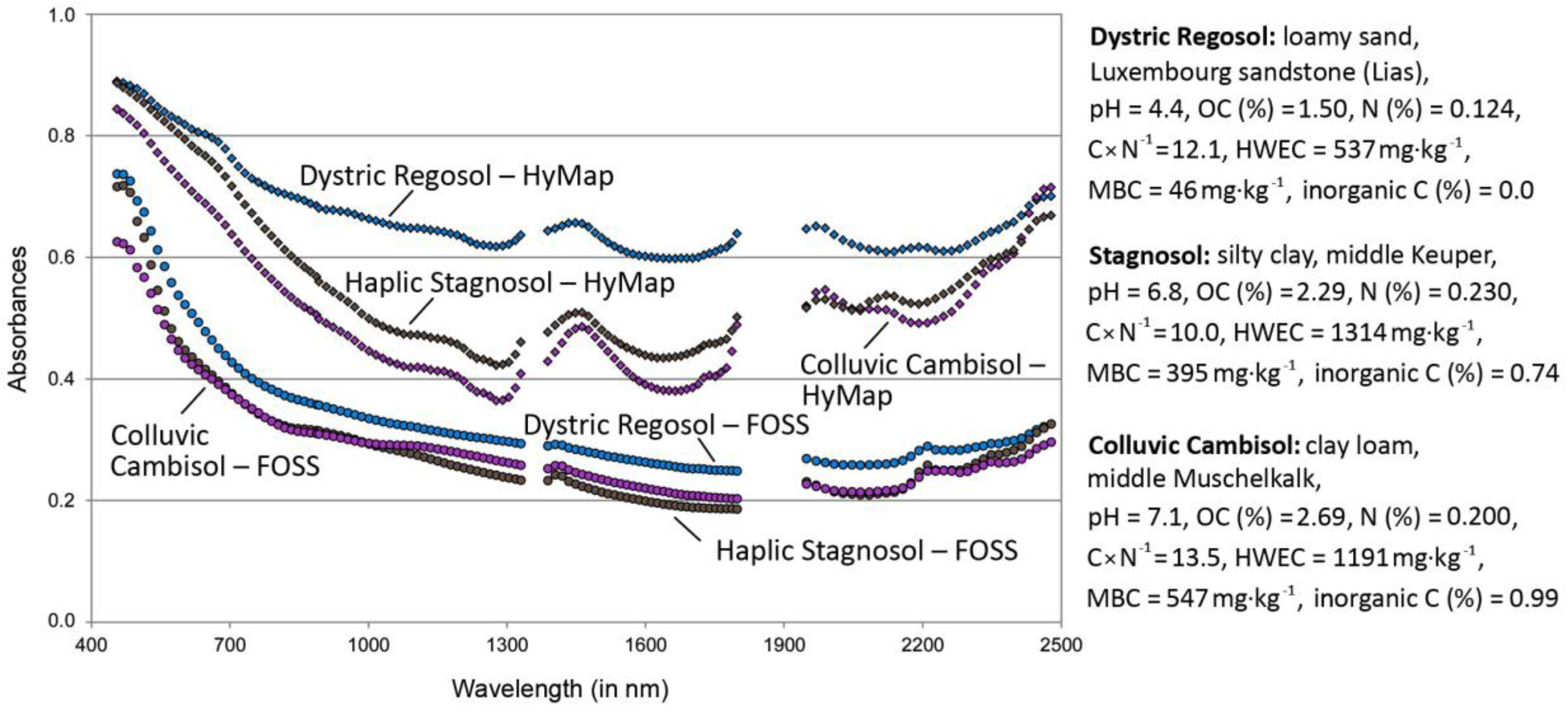
2.1. Study Site, Soil Samples and Their Analytical Properties

The study area (49°55′21.5′′N/6°25′05′′E–49°53′53.5′′N/6°45′52.5′′E) was located in the Bitburger Gutland, part of the Eifel low mountain range in Rhineland-Palatinate, Germany. The Bitburger Gutland forms a slightly undulating landscape with different plateaus between 300 and 450 m a.s.l., partly segmented by V-shaped and forested valleys in north to south direction. The plateaus are predominantly used by agriculture (Figure 1). Geologically, the Bitburger Gutland is mainly characterized by Triassic sediments that were deposited in the Trier-Bitburger basin (as an extension of the Parisian basin) (Figure 1); as a consequence of tectonic movements in the Neogene, different resistances to erosion have led to the formation of a series of escarpments [45].

In this region, we sampled a total of 60 agricultural plots with bare soils in a campaign between 23 and 27 August 2009. These plots were located in an area of 23 × 2.5 km², which represented the overflight stripe of the HyMap sensor (see Section 2.2). Plots influenced by clouds in the airborne image data were excluded, so that the data of 42 plots were finally used for the analysis in this study (Figure 1). They represented conventionally used arable land with regular plowing, typical crops being winter wheat, winter rape, rye and maize.

At the sampled plots, soils were classified according to the World Reference Base of Soil Resources [47]. The arable soils varied in the range of the parent materials (i.e., for example, debris from iron-rich sandstone, limestone, dolomite or clay sediments each overlain by layers with admixtures of loess) and were identified as Luvic and Haplic Stagnosols, Dystric, Eutric and Colluvic Cambisols, Dystric Regosols and Calcic Leptosols. Soil textures in topsoils (Ap horizons) ranged from (sample counts in parentheses) sand (2), to loamy sand (9), silty sand (8), sandy loam (2), silty loam and silt (11), clay loam (6) and silty clay (4). At each plot, soil was sampled from the top horizon (Ap, 0–10 cm depth). To this end, five samples were taken from one central point and four further sampling points at a distance of 1.5 m from the central point in each cardinal direction. All five samples per plot were pooled in one composite sample. For each plot, the central position was tracked with GPS.

In the laboratory, soil samples were sieved ≤2 mm, air-dried and, for C and N analyses, subsequently pulverized by grinding with an agate mortar. The pH was determined potentiometrically in a 0.01 M CaCl₂ solution with a glass electrode (soil-to-solution ratio 1:2.5). Total contents of OC and N were measured by gas chromatography after dry combustion at 1100 °C with a EuroEA elemental analyzer (HekaTech, Wegberg, Germany). Soil samples with possible free carbonate contents were pretreated to remove carbonate-C. In brief, 200 mg pulverized soil (dry matter basis) were treated with 200 mL 0.22 M HCl solution and then suspended (18,000 U min⁻¹) with an Ultra Turrax vortexer (IKA, Staufen, Germany) for at least three 3 min. Non-purgeable organic carbon equivalent to total organic carbon (TOC) was then analyzed from this suspension with a TOC-VCPN-analyzer (Shimadzu, Duisburg, Germany). HWEC was determined following the method of Körschens et al. [48]. After a 1-h extraction of 10 g soil with distilled water (50 mL) at 100 °C with a Gerhardt Turbotherm TT 125 (Gerhardt, Bonn, Germany), cooling, addition of MgSO₄ and centrifugation at 2600 rpm for 10 min, the dissolved organic carbon of the supernatant was analyzed with the Shimadzu TOC-VCPN-analyzer.

For soil microbiological analysis, the soil material was rewetted through the capillary method [49] using a spray bottle for gently sprinkling the samples twice a day for four days in total. MBC was determined by the chloroform fumigation extraction method according to Joergensen [50]; 0.01 M CaCl₂ solution was used to extract organic C from non-fumigated and chloroform-fumigated soil samples. Subsequent determination of C was performed with the Shimadzu TOC-VCPN analyzer. From the differential C content, MBC was calculated by using the correction factor kEC = 0.45 [50,51].

Statistics of the analyzed soil organic matter parameters (and pH values) are provided in

Table 1. Descriptive statistics of the parameters analytically determined for the studied 42 topsoil samples.

	Mean	Median	Range	Standard Deviation
OC (%)	1.76	1.56	1.09–3.01	0.49
N (%)	0.14	0.12	0.08–0.31	0.12
C × N−1	12.8	13.1	7.74–18.0	2.19
HWEC (mg·kg−1)	802	729	524–1314	221
MBC (mg·kg−1)	184	132	41.9–547	119
MBC × OC−1 (%)	0.98	0.84	0.28–2.03	0.45
Carbonate-C (%) a	0.16	0	0–1.55	0.36
pH (CaCl2)	5.29	5.80	4.33–7.23	0.86

^a 11 out of 42 samples contained carbonate.

. Correlations between the analyzed properties are shown in

Table 2. Correlation matrix (Pearson’s r) for studied soil properties (n = 42).

	N	HWEC	MBC
OC	0.80	0.76	0.78
N		0.88	0.82
HWEC			0.84

All correlations were significant at the p = 0.01 level.

. The samples covered a broad range of organic matter contents, C-N ratios and a soil reaction from strongly acidic to slightly alkaline pH values. In total, soil parameters given in Table 1 cover values that are typical for agricultural soils [52,53].

Selection of plots, sampling, wet-chemical analyses and spectral readings (see Section 2.2) provided the data pool for the further statistical analyses and the interpretation of the obtained results, as illustrated in Figure 2.

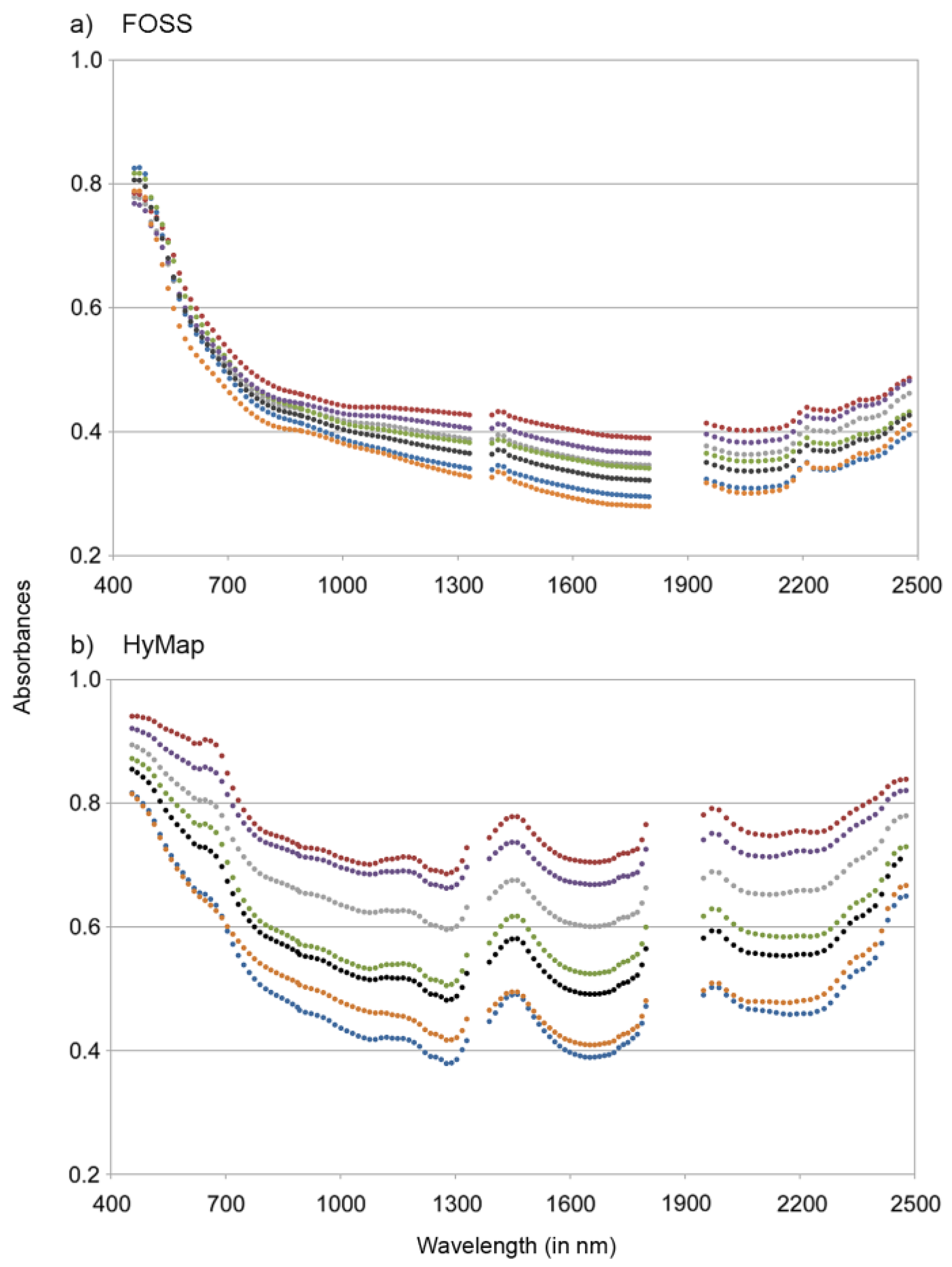
2.2. Spectral Database

A hyperspectral image was recorded with the 125-band HyMap airborne imaging sensor on 27 August 2009 near solar noon (solar zenith: 39.9°, solar azimuth: 180.7°). The band configuration of HyMap covered a wavelength range from 0.45 to 2.48 μm with band-specific FWHM (Full Width at Half Maximum of the spectral response function) values between 13 and 17 nm. The ground resolution realized in our dataset with a flight altitude of about 2290 m was approximately 4 m. A detailed description of the performance of HyMap in the laboratory can be found in Cocks et al. [54]; inter alia, HyMap achieves, while imaging a 50% reflectance target at an illumination zenith angle of 30 degrees, signal to noise ratios of about 1000:1 or better in spectral regions of the atmospheric windows.

The pre-processing of the acquired HyMap data included the following steps and provided a geocoded and atmospherically corrected image product containing surface reflectances:

-

conversion of digital numbers to at-sensor-radiances using laboratory and in-flight radiometric calibration data provided by HyVista Corporation (Baulkham Hills, Australia),

-

atmospheric correction to provide surface reflectances with the airborne ATCOR^® (ATCOR-4, German Aerospace Center DLR, Weßling, Germany) software based on the MODTRAN^® (MODerate resolution atmospheric TRANsmission) computer code,

-

parametric geocoding with the PARGE^® (ReSe Applications Schläpfer, Wil, Switzerland) software, that directly supports the processing of HyMap data and integrates flight parameters, terrain information and ground control reference points,

-

cross-track illumination correction (excluding forested and clouded areas) implemented in ENVI^TM (ENvironment for Visualizing Images, Harris Geospatial Solutions, Broomfield, CO, USA) using a second order polynomial approach.

Data calibration and atmospheric correction was performed by DLR (German Aerospace Center Oberpfaffenhofen, Weßling, Germany) as data provider. After pre-processing, those pixels were extracted which matched the field-measured GPS coordinates; the spectra of these pixels were transformed to (pseudo-)absorbances by log₁₀(reflectances⁻¹).

In the laboratory, Vis-NIR-SWIR spectra of all 42 air-dried and ground samples were collected with a FOSS XDS Rapid Content Analyzer (RCA) spectrometer (FOSS NIRSystems, Laurel, MD, USA), which combines a single beam monochromator with the RCA module containing the detectors. Measurements by the FOSS instrument are done in the diffuse reflectance mode. A tungsten halogen lamp is used as internal light source that irradiates, after a separation of the light into individual wavelengths by a holographic grating, the sample at normal incidence (0° zenith angle). The detectors of the RCA module are all mounted at a 45° angle to the sample surface. Scans are realized in the spectral range between 400 and 2500 nm with a sampling interval of 0.5 nm and a spectral resolution of 2 nm. The spectrometer is internally calibrated with a ceramic standard before each measurement [55,56]. In our case, soil samples were scanned in duplicate by placing them in a quartz-bottomed Petri dish on the sample window. The resulting spectra were recorded as (pseudo-)absorbances, obtained by log₁₀(reflectances⁻¹), and averaged over 32 scans for each sample. Finally, FOSS XDS spectra were resampled to HyMap spectral bands in which the spectral response function of each band was approximated by a Gaussian function.

Figure 3 shows, as examples, FOSS and HyMAP spectra measured and pre-processed for three different plots: one Dystric Regosol with high sand contents, low pH values (free of carbonates) and low OC contents, one clayey Stagnosol with higher pH values, higher contents of OC and inorganic C and a loamy Colluvic Cambisol with again slightly higher values for pH, OC and inorganic C.

2.3. Multivariate Calibrations of OC, N, MBC and HWEC from Spectral Measurements

PLSR based on the nonlinear iterative partial least squares algorithm (NIPALS) was used for the multivariate calibration of the studied soil properties from the pre-processed spectral datasets (FOSS and HyMap data, each with 125 spectral variables). PLSR was used with full spectra and in combination with CARS, IRIV and GA as different spectral variable selection techniques, which are described in short in the text below. The number of latent variables was defined in each case in a leave-one-out (LOO) cross-validation procedure with the minimum root-mean-square error (RMSE) as criterion; to reduce possible overfitting, we permitted a general maximum of twelve latent variables. As the limited total number of samples (n = 42) did not allow for a split into calibration and external validation samples, we performed alternatively an internal LOO cross-validation of the estimation model. However, one should be aware that LOO cross-validation might provide over-optimistic results, particularly when the number of samples is small. Accuracies may drop with independent validation samples [57,58].

Goodness of estimation was evaluated on the cross-validated (cv) results with the coefficient of determination (r²_cv), the ratio of performance to deviation (RPD_cv, defined as the ratio of standard deviation of the reference values to standard error of the cross-validated estimates), the RMSE_cv and the rRMSE_cv (relative RMSE_cv = RMSE_cv × measured arithmetic mean⁻¹).

CARS, here combined with PLSR, aims at selecting key wavelengths with a physical meaning [38,43] in a computationally efficient procedure, which is based on the obtained values of regression coefficients. In detail, a series of m sampling runs (m equaled 50 in our case) is performed, each with two selection steps. In the first step, an exponential function is used (with m and the number of original wavelengths as parameters) to define the number of spectral variables to be removed in each sampling run; the respective number of spectral variables with smallest regression coefficients is then excluded before the second step. In this second step, n random numbers are generated to pick a selection of those n variables that were kept in the first step. The probability of a variable to be picked with these random numbers refers to its weight that is directly related to its regression coefficient. At the end of this step, only those variables are kept that have been picked more than once. At the end of all sampling runs, the best model from the yet defined m models is chosen using the minimum RMSE in the LOO cross-validation. However, due to the random numbers in the second step, no unique solution exists. Thus, we used CARS in an ensemble mode, i.e., the complete procedure was repeated 30 times and the final results were obtained by averaging all 30 (generally normally distributed) predictions per sample.

Compared to CARS, IRIV follows a more exhaustive search strategy. Given the spectral data matrix with n samples and p variables a binary matrix with either 1 or 0 (in a ratio of 1:1) is generated; the dimension of this matrix is k × p with k as the number of random combinations of variables which is defined depending on the number of considered spectral variables. Each row of this binary matrix with a randomly generated sequence of 0 (variable is switched off) and 1 (variable is switched on) determines the variables that are used as input for PLSR. The performance of each subset (row) in the PLSR approach is then evaluated by the five-fold cross validated RMSE, so that a vector of RMSE_cv values with a dimension of k × 1 is obtained. In the next step, again all subsets defined by the rows of the binary matrix are considered for modeling, but now with systematic changes to assess the importance of each variable: Let us consider the first column (spectral variable) of the binary matrix; formerly 0, the value is now changed to 1 (and vice versa), while the state of all other variables in column 2, 3, …, p is not changed. Again, each subset (now changed at the first position) is used as input for PLSR. At the end of this step, we obtain k pairs of RMSE_cv, whereas each pair is related to one row of the binary matrix, one time including the first spectral variable (case A) and one time excluding it (case B). The average RMSE_cv is calculated for all case A- and all case B-models. If the mean RMSE_cv (A) is less than the mean RMSE_cv (B), the variable is considered informative. The described procedure is performed for all variables (columns) of the binary matrix. At the end, all informative variables are retained, while all other variables are removed. Then, a new binary matrix with a reduced dimension p is generated and the selection procedure starts again. As many rounds as necessary are performed so that only informative variables remain. Finally, a backward elimination is conducted with the retained informative variables to retrieve the final list of variables to be used in the PLSR approach. At this step, RMSE_cv is calculated with all retained (j) variables. Then it is tested whether leaving out another variable i (with i = 1, 2, …, j) provides a new minimum of RMSE_cv being smaller than RMSE_cv with all variables. If yes, this variable i is left out and the elimination strategy starts again (with j changed to j − 1); if no, no further variable is removed and the current list of variables is used for the final PLSR estimation procedure (with LOO cross-validation). Similar to CARS, IRIV does not provide a unique solution due to the use of random combinations of variables in the binary matrix. Thus, also with IRIV the complete cycle was repeated 30 times and the final results were averaged from all 30 outputs.

GAs are guided random search strategies inspired by natural selection mechanisms. The strategy is to select randomly an initial set of “chromosomes” (each with in our case 125 spectral variables (“genes”) and each gene switched on or off by binary coding) and then to generate new chromosomes by reproduction and mutation. The responses of the new chromosomes are evaluated (improved fitness or not?), which leads to a decision to include them in the population or to discard them. Response was here defined as the cross-validated percent of explained variance of the target variable obtained in the respective PLS regression. One hundred evaluations were performed in each run with a total number of 100 runs. At the end of all runs, the selected spectral variables of the overall fittest chromosome were identified as input for PLSR to retrieve estimates for the respective target soil variable. Detailed description of the GA algorithm used in this study can be found in Leardi [44]. Different from other GA algorithms, the performed runs are not independent from each other, but each run learns from the information (specified weights for each variable) brought by the previous runs. To combine both the benefits of this learning and the advantage of several independent solutions, we repeated the complete cycle of 100 runs 30 times. Final estimates with this method were then obtained by averaging all 30 solutions for each sample.

Finally, selections obtained with the different methods were “pooled”, i.e., all spectral variables (spectral bands) were ranked according to the selection frequencies obtained for them in CARS, IRIV and with the GA. For this ranking, the relative importance (RI) was calculated for each spectral variable and each of the studied soil properties according to (1):

$${\mathrm{RI}}_{(i=1,2,\dots ,125)}=\left(\frac{se{l}_{i,CARS}}{{\displaystyle \sum _{i=1}^{125}se{l}_{i,CARS}}}+\frac{se{l}_{i,IRIV}}{{\displaystyle \sum _{i=1}^{125}se{l}_{i,IRIV}}}+\frac{se{l}_{i,GA}}{{\displaystyle \sum _{i=1}^{125}se{l}_{i,GA}}}\right)\times \frac{1}{3}$$

(1)

where sel_i is the selection frequency for spectral variable i.

Spectral variables were then sorted according to their RI value and the respective measured spectral data were used in a forward selection mode for PLSR modeling. Estimates were then taken from the most successful model with the highest r² value in the cross-validation.

Based on the calculated RI values, the selection patterns were compared for the different soil properties. This was done for all 125 bands and, to consider multicollinearity, also for groups of wavelengths identified by a k-means clustering on the measured FOSS and HyMap data. Six groups were defined for FOSS (455–514 nm, 529–588 nm, 603–748 nm, 762–1207 nm, 1221–2331 nm, 2348–2478 nm), while HyMap data was clustered to seven groups (455–558 nm, 573–705 nm, 719–893 nm, 909–1193 nm, 1207–1405 nm and 1533–1776 nm, 1419–1519 nm and 1788–2331 nm, 2348–2478 nm). The distributions of RI values, now referred to these groups, were then compared one by one using chi²-statistics to identify similarities and significant differences between the different soil variables.

2.4. Indirect Assessment of MBC and HWEC from OC, N and with Modelled Spectra

In addition to PLSR, we also quantified MBC and HWEC in multiple linear regressions with N and OC as predictor variables. This analysis was done to explore the possible benefits of spectroscopic approaches for the quantification of these soil properties compared to a proxy approach with wet-chemical data. Again, a LOO cross-validation procedure was used to evaluate the predictive power of these regression models.

Besides this approach with only two predictor variables we also used PLSR that was applied to spectra not measured but fitted to the measured values of OC and N. The fitting procedure comprised (i) the selection of four samples—those with the minimum and the maximum values of OC and N—and their measured spectra; (ii) based on these four samples a linear regression analysis between OC and N (each four values) as x variables and the respective four spectral values (in each band) as y variable; and (iii) the application of the band-wise found regression coefficients for all other samples (n = 38) to model spectra as a fit to their measured OC and N contents (i.e., for each sample the spectral value in band i (with i = 1, 2,…, 125) was modeled with b₀ + b₁ × OC + b₂ × N). The retrieved spectra contained the complete spectral variability introduced by OC and N and preserved the typical shape of FOSS and HyMap spectra (Figure 4). The modeled spectra were then subjected to multivariate calibration to obtain estimates for all studied soil properties in a cross-validation approach.

3. Results

3.1. Estimation Results for Soil Variables from Measured Spectra

PLSR models based on full spectra without spectral variable selection provided the following order of accuracies for the FOSS laboratory measurements: OC >> N > MBC > HWEC (

Table 3. Statistics of estimates from FOSS and HyMap spectra using PLS regression with all 125 spectral variables (LOO cross-validated results).

Soil Property	FOSS (Laboratory)						HyMap (Airborne)
	l.V. a	r2cv	RMSEcv b	RPDcv	rRMSEcv	biascv c	l.V. a	r2cv	RMSEcv b	RPDcv	rRMSEcv	biascv c
	number of samples = 42
OC (%)	12	0.83	0.21	2.36	0.12	0.006	12	0.73	0.25	1.94	0.14	−0.005
N (%)	12	0.52	0.037	1.35	0.26	0.004	8	0.28	0.044	1.14	0.31	−0.0004
HWEC (mg·kg−1)	6	0.33	183	1.20	0.23	3.8	12	0.44	170	1.30	0.21	−4.7
MBC (mg·kg−1)	7	0.48	89	1.33	0.49	7.5	10	0.56	80	1.50	0.43	0.2
	number of samples = 41
OC (%)	12	0.79	0.23	2.11	0.13	0.001	11	0.71	0.26	1.89	0.15	−0.007
N (%)	10	0.68	0.029	1.77	0.20	0.001	12	0.49	0.037	1.35	0.26	−0.0002
HWEC (mg·kg−1)	10	0.53	155	1.41	0.19	−9.8	12	0.53	155	1.42	0.19	−16.3
MBC (mg·kg−1)	7	0.61	76	1.57	0.41	4.1	12	0.73	62	1.94	0.33	−0.6

^a number of latent variables; ^b units are given in the first column; ^c bias_cv (mean error) = mean of cross-validated estimates—mean of measured values, units are given in the first column.

). With the exception of OC, results were weak, with RPD values less than 1.5 in the LOO cross-validation. For HyMap data, the order was OC > MBC > HWEC > N; results for OC and N were worse than with the FOSS data, while estimates for MBC and HWEC, although at a low accuracy level, were slightly more accurate than with FOSS (Table 3).

The analysis of the FOSS results showed that one certain sample provided the markedly highest error terms for N, MBC and HWEC. In an outlier analysis performed in the spectral feature space, this sample was indicated as being the only outlier with a Mahalanobis distance at H = 18.5 and a p-value < 0.01 when compared to the chi² probability distribution function. Excluding this sample improved estimation accuracies for N, HWEC and MBC considerably for both FOSS and also HyMap data (Table 3). However, the respective outlier analysis on HyMap data did not indicate any outlier, so that the further analysis using PLSR combined with spectral variable selection was performed with all 42 samples.

Estimation accuracies improved considerably when PLSR was combined with spectral variable selection techniques (

Table 4. Statistics of estimates from FOSS and HyMap spectra using PLSR combined with different spectral variable selection methods (LOO cross-validated results, n = 42).

	Selection Method	FOSS (Laboratory)						HyMap (Airborne)
		l.V. b	r2cv	RMSEcv c	RPDcv	rRMSEcv	biascv d	l.V. b	r2cv	RMSEcv c	RPDcv	rRMSEcv	biascv d
OC a	CARS	9 (15)	0.89	0.16	3.06	0.09	<0.001 *	10 (24)	0.76	0.24	2.04	0.14	−0.006
	IRIV	11 (19)	0.93	0.13	3.72	0.07	0.004	9 (22)	0.76	0.24	2.05	0.13	−0.001
	GA	9 (11)	0.94	0.12	4.08	0.07	0.002	10 (14)	0.85	0.19	2.62	0.11	−0.004
	pooled	10 (36)	0.89	0.16	3.08	0.09	0.007	10 (63)	0.79	0.22	2.20	0.13	−0.005
N a	CARS	9 (12)	0.80	0.023	2.21	0.16	>−0.001 *	7 (12)	0.55	0.033	1.50	0.23	>−0.001 *
	IRIV	9 (13)	0.81	0.021	2.34	0.15	<0.001 *	6 (8)	0.57	0.033	1.54	0.23	>−0.001 *
	GA	10 (11)	0.93	0.014	3.70	0.10	<0.001 *	7 (9)	0.70	0.027	1.86	0.19	>−0.001 *
	pooled	9 (14)	0.78	0.023	2.15	0.16	−0.001 *	8 (9)	0.52	0.035	1.43	0.25	0.001
HWEC a	CARS	9 (15)	0.60	138	1.59	0.17	>−1 *	7 (11)	0.67	125	1.76	0.16	1
	IRIV	5 (9)	0.42	166	1.33	0.21	6	8 (11)	0.63	134	1.65	0.17	>−1 *
	GA	5 (5)	0.73	114	1.94	0.14	1	11 (14)	0.86	82	2.68	0.10	1
	pooled	10 (10)	0.64	131	1.68	0.16	<1	12 (17)	0.67	128	1.72	0.16	3
MBC a	CARS	8 (8)	0.70	64	1.85	0.35	1.0	10 (21)	0.72	62	1.92	0.34	−0.6
	IRIV	7 (15)	0.78	56	2.13	0.30	2.2	10 (20)	0.83	48	2.49	0.26	<0.1 *
	GA	7 (7)	0.84	48	2.50	0.26	1.5	10 (12)	0.86	44	2.68	0.24	−0.5
	pooled	12 (14)	0.81	51	2.32	0.28	0.4	9 (19)	0.80	51	2.35	0.28	−0.2

^a OC and N in %, HWEC and MBC in mg kg⁻¹; ^b number of latent variables, in case of CARS, IRIV and GA averaged from 30 runs; in brackets number of selected original spectral variables; ^c units are given in the first column; ^d bias_cv (mean error) = mean of cross-validated estimates—mean of measured values, units are given in the first column; * between given value and 0.0.

). With FOSS data, RPD_cv obtained for OC was greater than 3.0 in all cases. Results were worst for HWEC with RPD_cv values being generally less than 2.0. Compared to FOSS results, accuracies dropped distinctly on HyMap data for OC and N, but remained stable or even improved for MBC and HWEC. Similar to PLSR results without variable selection, the order of accuracies obtained with CARS, IRIV and GA switched from OC > N > MBC > HWEC (FOSS) to OC, MBC > HWEC (at least for CARS and IRIV) > N (HyMap).

From all applied selection techniques, GA was the most successful one for all soil variables and for both FOSS and HyMap data (Table 4). Differences between GA and the other selection approaches were most pronounced for N (with FOSS data, RPD_cv at 3.70 and less than 2.5 for all other methods) and HWEC (with HyMap data, RPD_cv at 2.68 and less than 2.0 with other methods). With pooled selections, accuracies of obtained results usually ranked in the mid-range; only for N this approach was slightly inferior to the other selection procedures (Table 4). In most cases, with the exception of N and HWEC (CARS), less spectral variables were selected on the laboratory data compared to HyMap data (Table 4).

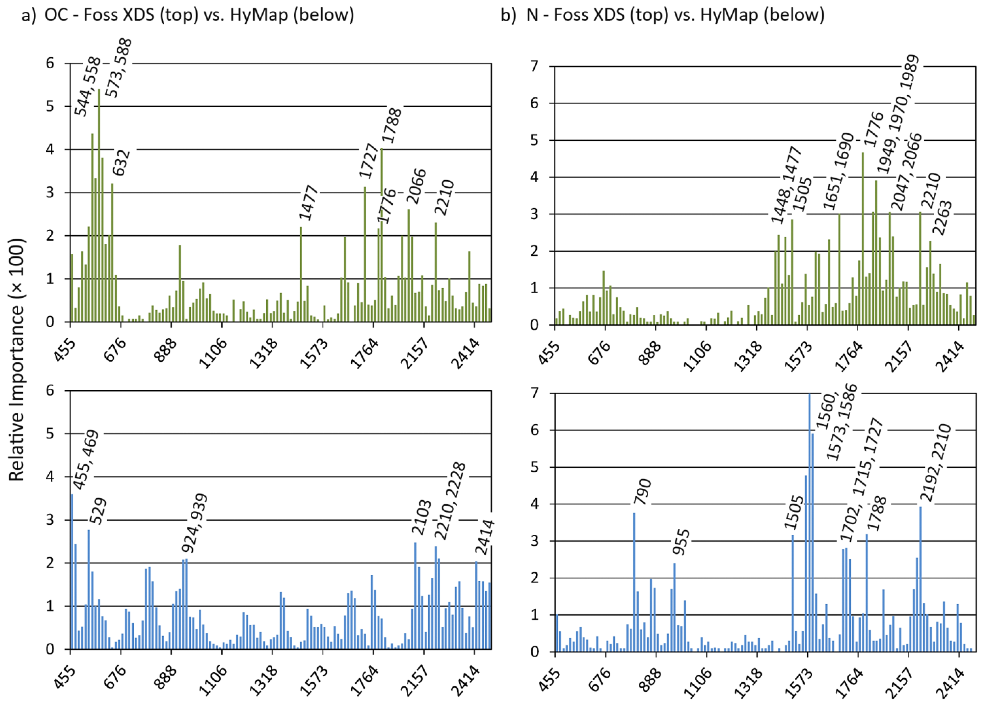
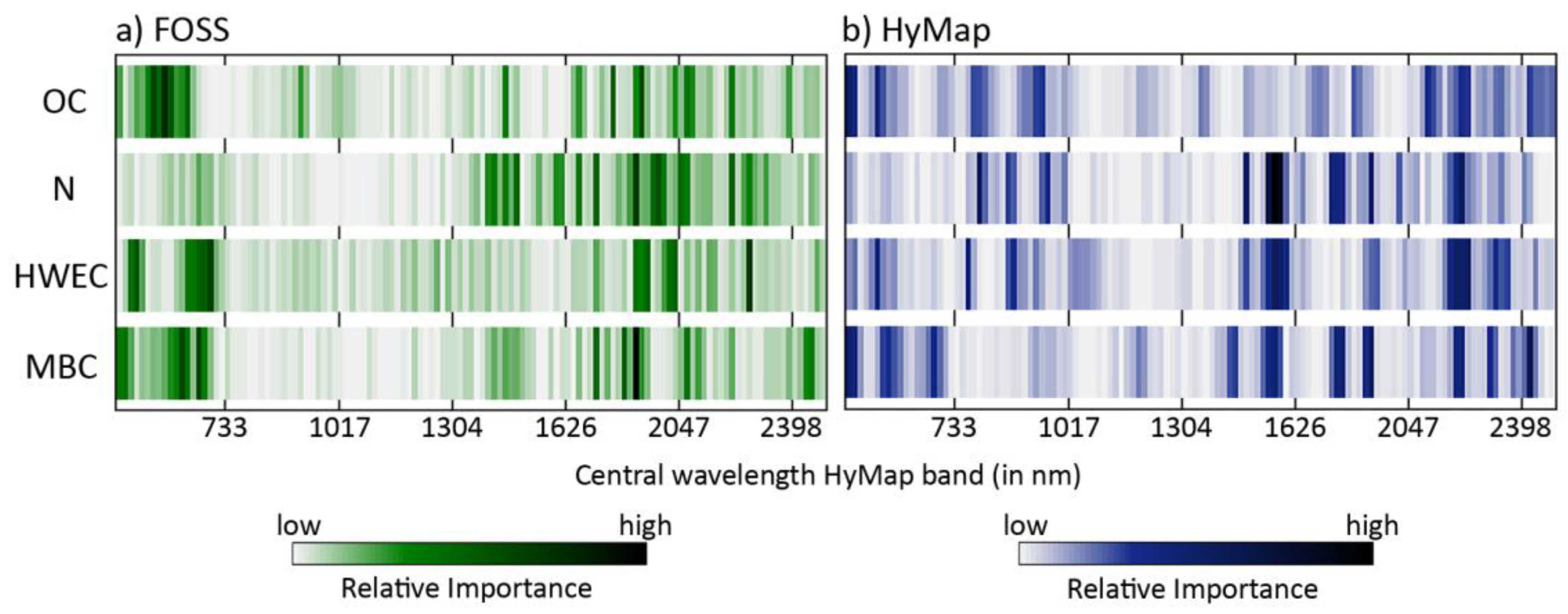
3.2. Analysis of Selection Patterns

As the RI integrates the results of CARS, IRIV and GA, it was analyzed for all 125 spectral variables to elucidate differences from one soil variable to another and between FOSS and HyMap. For the comparison between HyMap and FOSS, we found marked differences for all soil variables, being less pronounced for OC compared to N (both illustrated in detail by Figure 5). For an easy comparison, Figure 6 shows relative RI values for all data.

In the case of OC, spectral values in the visible range and in the SWIR beyond 2050 nm were important for the PLSR approach on both laboratory and airborne data. Differences between both were more pronounced in the NIR range from 700 to 1000 nm (which was of greater relevance for the HyMap data) and the SWIR range below 2050 nm with some marked RI peaks only for the laboratory data measured with the FOSS instrument (Figure 5a). Values in the NIR between 1000 and 1300 nm were irrelevant for both datasets. For N, a series of marked RI peaks were found for both laboratory and airborne data in the SWIR range at wavelengths greater than 1400 nm, but with the exceptions of 1505 and 2210 nm the positions of these peaks did not match (Figure 5b). In addition, the NIR range below 1000 nm was relevant for the modeling on HyMap data, but of no meaning for the laboratory data. For HWEC, the importance of the spectral region less than 700 nm markedly differed between FOSS and HyMap data, whereas this region was relevant for MBC on both datasets (Figure 6). For both variables, some NIR and SWIR key wavelengths on HyMap were of low importance for the FOSS data (HWEC: 1560–1599 nm; MBC: 1560, 1573, 2210 and 2297 nm; Figure 6 and

Table 5. Wavelengths with high RI values (RI > 0.02) identified on FOSS XDS and HyMap data for HWEC and MBC (Vis: 400–700 nm, NIR: >700–1300 nm, SWIR: >1300–2500 nm; central wavelengths (rounded to the nearest nm value) of the respective HyMap bands are given).

	FOSS XDS (Laboratory)		HyMap (Airborne)
HWEC	Vis: SWIR:	484, 499, 632, 647, 661, 676, 690 1776, 1788, 1798, 2008, 2027, 2263	Vis: SWIR:	529, 762, 875 1560, 1573, 1586, 1599, 2175, 2192, 2210, 2228, 2314
MBC	Vis: SWIR:	455, 469, 588, 603, 618, 632, 661, 676 1690, 1752, 1776, 2066, 2430, 2447	Vis: SWIR:	455, 469, 544, 558, 676 1477, 1560, 1573, 1715, 1727, 1776, 1788, 2192, 2210, 2297, 2414

No high RI values were in the NIR region.

).

Concerning RI peaks, we found some bands with a general relevance for all four constituents (Figure 6, Table 5): The band at 2210 nm, usually attributed to the OH combination band of clay minerals [59], was markedly prominent with peaks for OC, N (FOSS and HyMap data), and, on HyMap data, for HWEC and MBC. Absorbances measured at 1776 nm were of importance in the laboratory for all constituents, spectral values at 632 nm for OC, HWEC and MBC. For HyMap, values at 1560, 1573 and 2192 nm were identified as being important for N, HWEC and MBC; these wavelengths may be related to the combination band of free or adsorbed soil water located at 1450 nm (see also Figure 3 for the relevance of this band in the HyMap data) and again to the clay hydroxyl band around 2200 nm [59,60].

Based on grouped spectral variables (see Section 2.3), Chi²-statistics indicated highly significant differences between the distributions of RI obtained with FOSS for OC, N, HWEC and MBC (p < 0.01 in all cases, with the exception of MBC compared to HWE with lower but still significant differences at p = 0.019). Results differed for HyMap in a way that OC and HWEC showed similar distributions (p = 0.33); in all other cases, differences were again highly significant (with p < 0.01).

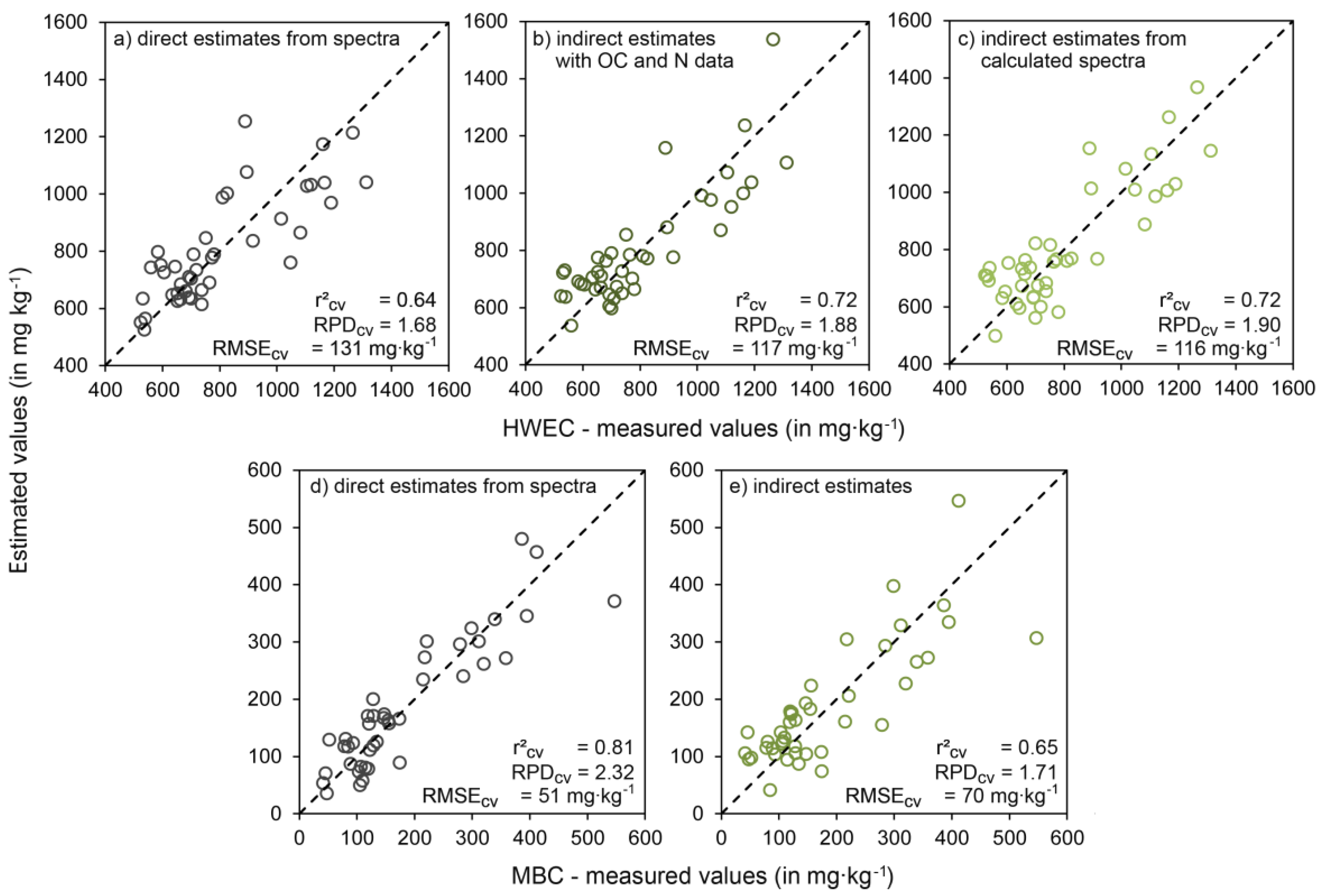
3.3. Indirect Approaches to Quantify HWEC and MBC

We used both measured and estimated values of OC and N to predict HWEC and MBC (

Table 6. Statistics of estimates for HWEC and MBC obtained with multiple linear regression (measured and estimated values for OC and N as predictors *) and with PLSR using modeled spectra (LOO cross-validated results, n = 42).

Soil Property	Predictors	r2cv	RMSEcv a	RPDcv	rRMSEcv	biascv b
HWEC	chemical data (OC, N)	0.72	117	1.88	0.15	2
(mg·kg−1)	estimates of OC, N (obtained with FOSS 1)	0.58	143	1.55	0.18	−1
	estimates of OC, N (obtained with HyMap 1)	0.57	142	1.55	0.18	−2
	modeled FOSS spectra 2	0.72	116	1.90	0.15	1
	modeled HyMap spectra 2	0.72	117	1.88	0.15	2
MBC	chemical data (OC, N)	0.65	70	1.71	0.38	0.7
(mg·kg−1)	estimates of OC, N (obtained with FOSS 1)	0.59	76	1.56	0.41	0.4
	estimates of OC, N (obtained with HyMap 1)	0.48	85	1.40	0.46	−0.5
	modeled FOSS spectra 2	0.65	70	1.71	0.38	0.7
	modeled HyMap spectra 2	0.65	70	1.71	0.38	0.7

* predictors were significant with p-values < 0.05 in all cases; ¹ estimates of OC and N obtained with PLSR and pooled selected variables; ² as described in Section 2.4; ^a units are given in the first column; ^b bias_cv (mean error) = mean of cross-validated estimates—mean of measured values, units are given in the first column.

). For both variables, measured values were generally more appropriate than estimated values. For HWEC, wet-chemical data of OC and N provided estimates that were more accurate than the results obtained with almost all spectrally based approaches (Table 3, Table 4 and Table 6), in which the indirect approach was only outperformed by GA-PLSR applied to laboratory and airborne data. In case of MBC, the indirect approaches using values of OC and N did not reach the accuracies of PLSR combined with variable selection, independent from the selection method and the data (laboratory and airborne, Table 4).

The use of modeled spectra that had been fitted to measured OC and N values as input for PLSR provided perfect estimates for both, OC and N (with modeled FOSS as well as with modeled HyMap spectra; r²_cv = 1, each with three latent variables). Using these spectra for the estimation of HWEC and MBC supported the results obtained with linear regression using wet-chemical data of OC and N (Table 6). With modeled FOSS spectra, HWEC was estimated with r²_cv = 0.72, RMSE_cv = 116 and RPD_cv = 1.90 (Table 6, Figure 3), based on modeled HyMap spectra results were almost identical (Table 6). Visualization of measured vs. estimated HWEC values in a scatterplot documents that the indirect approaches—with chemical data and especially with calculated spectra—outperformed a direct estimation from measured spectra with respect to accuracy and also more homoscedastic residues (Figure 7). In total, these results indicate a very limited use of direct spectral approaches for this soil variable. In contrast, estimates of MBC obtained with indirect approaches showed more scattering around the 1-1 line than those that were quantified from the measured spectra (Figure 7).

4. Discussion

This study confirmed that OC, which is one key soil characteristic, could be estimated with success using airborne IS. The results are well in line with results of other studies, e.g., Steinberg et al. [8] (r²_cv = 0.74, RPD_cv = 1.90) or Hbirkou et al. [6] (r²_cv = 0.83, RPD_cv = 2.45). However, OC could not be predicted with HyMap spectra in the study of Gomez et al. [5] (r²_cv = 0.02, RPD_cv = 0.99), which was probably due to low OC contents (between 0.4 and 1.5%) in their calibration data. Stevens et al. [61], who studied airborne data of the AHS-160 sensor (Argon ST, Ann Arbor, MI, USA) for the retrieval of OC, worked out that in case of heterogeneous soil conditions stratified approaches referring to sub-regions or, even more appropriate, to different soil types are reasonable for a further improvement of estimation accuracies; for example, with PLSR and based on 100 validation samples examined in that study, accuracies improved from r²_cv = 0.53 and RPD_cv = 1.47 in a “global” approach without stratification to r²_cv = 0.86 and RPD_cv = 2.76 based on soil type specific sub-models. This goes in line with the findings of Colombo et al. [62], who propose to classify soil samples according to their main pedological features followed by the calibration of specific PLS models. This kind of stratification would also be an option for the heterogeneous soil region studied here, in case of a greater number of available samples. Selige et al. [7] used HyMap data and obtained estimates of high accuracy for both OC and total N (r²_cv = 0.90 and r²_cv = 0.92), in which especially the results for N outperformed our results markedly. The latter could, in part, be due to a very high correlation between OC and N in the dataset of Selige et al. [7]—Pearson’s r equaled 0.97 compared to 0.80 in our data.

For HWEC and MBC, comparative data of other airborne IS studies are not available. For both variables, estimates from HyMap data were generally more accurate than those from FOSS data. However, PLSR combined with pooled variable selections yielded only very small differences. Deviating from that, estimates of OC and N were markedly less accurate when using HyMap instead of laboratory data. The latter is in line with the findings of Stevens et al. [9], who also compared laboratory (ASD FieldSpec) and airborne (AHS-160 sensor) hyperspectral data and found markedly reduced accuracies for OC on the image level—RPD_cv dropped from 2.03 (lab) to 1.47 (image). Similar to this, Lagacherie et al. [10] found for the example of HyMap data that empirical relations between laboratory spectra and soil variables (clay and calcium carbonate contents) distinctly degraded to the image level; estimation accuracies obtained from both datasets differed accordingly. Different data levels or scales (laboratory vs. image) are indicated by systematic variations of the shapes of the measured spectra, as discussed in detail by Stevens et al. [9]. Different shapes were also obvious for our data (Figure 3 and Figure 4), although some typical absorption features were notable in both datasets (absorption peaks for carbonate at 2350 nm and for clay around 2200 nm [2,10]) and different general reflectance levels due to different soil textures (decreasing reflectances with increasing particle sizes) were also apparent (Figure 3). Remote but direct measurements of more or less rough topsoil surfaces with HyMap are basically different from lab measurements using prepared (dried and ground) samples; increasing soil roughness reduces reflectances due to the effects of microshades, so that absorbance values of laboratory data were markedly lower than those recorded by the HyMap sensor. Spectrally, HyMap provides contiguous sampling without covering the strong atmospheric water absorption bands near 1380 and 1875 nm [63]. However, water absorption bands occurring adjacently to water vapor bands with peaks at 1940 nm, 1450 nm and also, weaker and broader than the other two bands, at 1200 nm [63], markedly influenced the shape of the HyMap spectra (Figure 3 and Figure 4). In addition, vegetation coverage or crop residues are also spectrally meaningful factors [9], but not of high relevance here, as we only considered bare soils without or with very little crop residues or stubble. We thus consider different soil moisture contents and soil surface roughnesses to be the main factors for the variability of the HyMap compared to the FOSS spectra. In addition, radiometric calibration uncertainties of the HyMap sensor, possible residual atmospheric effects [10] and not fully compensated directional effects of the monitored soil surfaces may have also induced general spectral differences between airborne and laboratory data.

The reduced variability of FOSS spectra compared to HyMap spectra explains why in most cases (see Section 3.1) less spectral variables were selected on the laboratory data. Selection patterns differed between both datasets. In all cases, variable selection improved estimation accuracies markedly, most pronounced for OC, N and MBC on FOSS data. With pooled selections, RPD_cv increased to values greater than 2.0 for MBC (both datasets), N (lab) and OC (HyMap); on laboratory scale, RPD_cv obtained for OC increased from 2.36 to more than 3.0.

Despite the differences between laboratory and HyMap spectra, we identified some key wavelengths being highly prominent for the quantification of the studied soil variables, above all the hydroxyl band around 2200 nm. This coincides with the findings for other datasets, for example by Viscarra-Rossel and Behrens [34] (OC), Vohland and Emmerling [64] (OC and HWEC) or Vohland et al. [65] (OC, N). In these studies, the water band at 1940 nm was also identified as key region for OC, N and HWEC, but in the data here this only applied for N on the level of laboratory spectra. However, the second important water band at 1450 nm was identified as key region for OC, N (laboratory data) and MBC (HyMap data). Stenberg et al. [59] provide a detailed overview of main soil organic constituents and their overtone and combination bands in the NIR region; bands around 1100, 1600, 1700 to 1800, 2000 and 2200 to 2400 nm were reported to be particularly relevant for OC and N calibration. In addition to the hydroxyl band around 2200 nm, we found a match for the 1700 to 1800 nm region for OC and N in the laboratory data, for N also in the HyMap data, which may be attributed to an alkyl band in this spectral region [34]. In line with previous studies [59], we found the visible region to be important for the assessment of OC.

Accuracies obtained for the estimation of HWEC and MBC differed distinctly in our study. However, for both it was hypothesized that their spectral prediction may be closely coupled to that of spectrally active main soil properties. For MBC, Zornoza et al. [16] discussed this issue with a focus an OC as main factor. Values of r² obtained in a simple linear regression between measured OC and MBC values were lower than the r² values obtained for MBC in the multivariate estimation procedure using NIR data and PLSR. Furthermore, spectral ranges used for the multivariate calibration of OC and MBC differed markedly. From these findings the authors concluded that specific information for MBC must be contained in the spectra. Ludwig et al. [66,67] showed that other main soil properties, in addition to OC, were also relevant for the quantification of MBC. Depending on the sample set, they found the following predictor variables to add significantly to the quantification of MBC in multiple linear regressions: (N, pH, clay), (pH, sulphur (S)), (OC, pH) and (OC, N, S, phosphorus (P)). Estimates with these variables were almost as successful as those with spectral data (whereby mid-infrared data in the range between 400 and 7000 cm⁻¹ and not Vis-NIR-SWIR data were used in these studies). However, from the fact that the most appropriate set of predictor variables differed from one sample set to the other, it can be concluded that underlying predictive mechanisms were variable and prediction models could not be transferred in space and time. This is also in line with the findings of other studies [68,69]. Emmerling and Udelhoven [68] modeled MBC of agricultural soils with multiple regressions based on other soil properties and identified clay content, pH and HWEC as highly significant predictors. The application of their model to another dataset provided marked underestimates of MBC, better results were obtained by considering clay content, organic matter, pH and annual precipitation values or by a combination of OC, N, clay and sand content [69]. However, these results also indicate that a combination of spectral and non-spectral predictors may be promising, which was realized for example by Peng et al. [70] (though not for biological soil properties), who used laboratory spectral data combined with ancillary environmental data (e.g., plant available water, soil texture classes) and spectral indices based on multispectral remote sensing data for the quantification and spatial modeling of OC.

For HWEC, indirect approaches (i.e., a multiple linear regression with OC and N as predictors and PLSR based on spectra calculated from OC and N values) were more successful than direct approaches based on measured spectra—with PLSR or even PLSR combined with CARS, IRIV and pooled selected variables. Furthermore, spectral variable selection patterns calculated for HyMap did not deviate significantly between HWEC and OC. These findings indeed indicate a very limited use of Vis-NIR-SWIR data, both laboratory and airborne, for a direct quantification of HWEC. No overall spectral pattern was found for HWEC, which may also result from the large variability and heterogeneity of this pool, as it consists of large portions of easily degradable compounds such as carbohydrates, peptides and amino acids [30,71].

For MBC the findings were different: Pattern analysis of selected variables indicated significant differences from those of OC, N and also HWEC. Indirect approaches were outperformed by PLSR coupled to any of the spectral variable selection methods, especially in combination with IRIV, GA and pooled selections. This even did not change with the integration of measured pH values in the multiple linear regression in addition to OC and N (as proposed by the findings of Ludwig et al. [66,67]), which improved accuracy of indirect MBC estimates only slightly (r²_cv = 0.68, RPD_cv = 1.77, RMSE_cv = 0.37). This all suggests specificity of the spectral information for MBC, which may either result from a direct and own spectral signature or from a complex interaction of other spectrally meaningful factors related to MBC (or from a combination of both).

5. Conclusions

Airborne IS proved appropriate for the quantification of key soil properties, above all OC and MBC. Shape of spectra indicated marked differences between the laboratory level (prepared samples) and airborne observations (bare soil surfaces), as the latter was influenced by more variable on-site conditions. Empirical approaches applied with success on laboratory spectroscopic data are thus not per se ready to be employed for airborne data or even hyperspectral spaceborne data, as, for example, the forthcoming Environmental Mapping and Analysis Programme (EnMAP) or the Hyperspectral and Infrared Imager (HyspIRI) missions. With coarser spatial resolutions achieved by the satellite missions, pure bare soil pixels will be more unlikely and approaches are needed to cope with mixed pixels. In any case, estimation models should be re-calibrated for each new situation and for changing conditions defined through soil moisture, roughness and possibly crop residues.

The combination of PLSR with spectral variable selection is a valuable tool for improving accuracies of the obtained estimates. This was shown for conceptually different approaches and proved valid for a more generalized procedure with pooled selections, which balanced the specific responses of the individual methods. Identified key variables could in part be interpreted physically and related to the absorption band of free or adsorbed soil water around 1450 nm and the hydroxyl band around 2200 nm.

Based on our results, the spectral approach is beneficial for the quantification of MBC (but not for HWEC), as it outperformed the indirect approaches with OC and N as predictor variables and/or with calculated spectra being ideal for the measured OC and N values. Specificity of the spectra was identified, but the underlying spectral principles that yield the potential for a statistical prediction of MBC cannot be fully understood from the analysis of one sample set. For this, a comparative analysis with a great number of sample sets with highly different spectral properties and a very wide range of couplings between physical, chemical and biological soil properties would be advisable.

References

1. Cécillon, L.; Barthès, B.G.; Gomez, C.; Ertlen, D.; Genot, V.; Hedde, M.; Stevens, A.; Brun, J.J. Assessment and monitoring of soil quality using near-infrared reflectance spectroscopy (NIRS). Eur. J. Soil Sci. 2009, 60, 770–784. [Google Scholar] [CrossRef]
2. Chabrillat, S.; Goetz, A.F.H.; Krosley, L.; Olsen, H.W. Use of hyperspectral images in the identification and mapping of expansive clay soils and the role of spatial resolution. Remote Sens. Environ. 2002, 82, 431–434. [Google Scholar] [CrossRef]
3. Franceschini, M.H.D.; Demattê, J.A.M.; da Silva Terra, F.; Vicente, L.E.; Bartholomeus, H.; de Souza Filho, C.R. Prediction of soil properties using imaging spectroscopy: Considering fractional vegetation cover to improve accuracy. Int. J. Appl. Earth Obs. 2015, 38, 358–370. [Google Scholar]
4. Wight, J.P.; Ashworth, A.J.; Allen, F.L. Organic substrate, clay type, texture, and water influence on NIR carbon measurements. Geoderma 2016, 261, 36–43. [Google Scholar] [CrossRef]
5. Gomez, C.; Lagacherie, P.; Coulouma, G. Regional predictions of eight common soil properties and their spatial structures from hyperspectral Vis-NIR data. Geoderma 2012, 189–190, 176–185. [Google Scholar] [CrossRef]
6. Hbirkou, C.; Pätzold, S.; Mahlein, A.K.; Welp, G. Airborne hyperspectral imaging of spatial soil organic carbon heterogeneity at the field scale. Geoderma 2012, 175–176, 21–28. [Google Scholar] [CrossRef]
7. Selige, T.; Böhner, J.; Schmidhalter, U. High resolution topsoil mapping using hyperspectral image and field data in multivariate regression modeling procedures. Geoderma 2006, 136, 235–244. [Google Scholar] [CrossRef]
8. Steinberg, A.; Chabrillat, S.; Stevens, A.; Segl, K.; Foerster, S. Prediction of common surface soil properties based on Vis-NIR airborne and simulated EnMAP imaging spectroscopy data: Prediction accuracy and influence of spatial resolution. Remote Sens. 2016, 8, 613. [Google Scholar] [CrossRef]
9. Stevens, A.; van Wesemael, B.; Bartholomeus, H.; Rosillon, D.; Tychon, B.; Ben-Dor, E. Laboratory, field and airborne spectroscopy for monitoring organic carbon content in agricultural soils. Geoderma 2008, 144, 395–404. [Google Scholar] [CrossRef]
10. Lagacherie, P.; Baret, F.; Feret, J.-B.; Madeira Netto, J.; Robbez-Masson, J.-M. Estimation of soil clay and calcium carbonate using laboratory, field and airborne hyperspectral measurements. Remote Sens. Environ. 2008, 112, 825–835. [Google Scholar] [CrossRef]
11. Ben-Dor, E.; Patkin, K.; Banin, A.; Karnieli, A. Mapping of several soil properties using DAIS-7915 hyperspectral scanner data—A case study over clayey soils in Israel. Int. J. Remote Sens. 2002, 23, 1043–1062. [Google Scholar] [CrossRef]
12. Chang, C.W.; Laird, D.A.; Mausbach, M.J.; Hurburgh, C.R.J. Near-infrared reflectance spectroscopy–principal components regression analyses of soil properties. Soil Sci. Soc. Am. J. 2001, 65, 480–490. [Google Scholar] [CrossRef]
13. Chodak, M. Near-infrared spectroscopy for rapid estimation of microbial properties in reclaimed mine soils. J. Plant Nutr. Soil Sci. 2011, 174, 702–709. [Google Scholar] [CrossRef]
14. Heinze, S.; Vohland, M.; Joergensen, R.G.; Ludwig, B. Usefulness of near-infrared spectroscopy for the prediction of chemical and biological soil properties in different long-term experiments. J. Plant Nutr. Soil Sci. 2013, 176, 520–528. [Google Scholar] [CrossRef]
15. Terhoeven-Urselmans, T.; Schmidt, H.; Joergensen, R.G.; Ludwig, B. Usefulness of near-infrared spectroscopy to determine biological and chemical soil properties: Importance of sample pre-treatment. Soil Biol. Biochem. 2008, 40, 1178–1188. [Google Scholar] [CrossRef]
16. Zornoza, R.; Guerrero, C.; Mataix-Solera, J.; Scow, K.M.; Arcenegui, V.; Mataix-Beneyto, J. Near infrared spectroscopy for determination of various physical, chemical and biochemical properties in Mediterranean soils. Soil Biol. Biochem. 2008, 40, 1923–1930. [Google Scholar] [CrossRef] [PubMed]
17. Bastida, F.; Zsolnay, A.; Hernández, T.; García, C. Past, present and future of soil quality indices: A biological perspective. Geoderma 2008, 147, 159–171. [Google Scholar] [CrossRef]
18. Ritz, K.; Black, H.I.J.; Campbell, C.D.; Harris, J.A.; Wood, C. Selecting biological indicators for monitoring soils: A framework for balancing scientific and technical opinion to assist policy development. Ecol. Indic. 2009, 9, 1212–1221. [Google Scholar] [CrossRef] [Green Version]
19. Pulleman, M.; Creamer, R.; Hamer, U.; Helder, J.; Pelosi, C.; Pérès, G.; Rutgers, M. Soil biodiversity, biological indicators and soil ecosystem services—An overview of European approaches. Curr. Opin. Sust. 2012, 4, 529–538. [Google Scholar] [CrossRef] [Green Version]
20. Velasquez, E.; Lavelle, P.; Andrade, M. GISQ, a multifunctional indicator of soil quality. Soil Biol. Biochem. 2007, 39, 3066–3080. [Google Scholar] [CrossRef]
21. Havlicek, E. Soil biodiversity and bioindication: From complex thinking to simple acting. Eur. J. Soil Biol. 2012, 49, 80–84. [Google Scholar] [CrossRef]
22. Böhme, L.; Langer, U.; Böhme, F. Microbial biomass, enzyme activities and microbial community structure in two European long-term field experiments. Agric. Ecosyst. Environ. 2005, 109, 141–152. [Google Scholar] [CrossRef]
23. Fließbach, A.; Oberholzer, H.-R.; Gunst, L.; Mäder, P. Soil organic matter and biological soil quality indicators after 21 years of organic and conventional farming. Agric. Ecosyst. Environ. 2007, 118, 273–284. [Google Scholar] [CrossRef]
24. Hoyle, F.C.; Murphy, D.V.; Fillery, I.R.P. Temperature and stubble management influence microbial CO2-C evolution and gross transformation rates. Soil Biol. Biochem. 2006, 38, 71–80. [Google Scholar] [CrossRef]
25. Lundquist, E.J.; Scow, K.M.; Jackson, L.E.; Uesugi, S.L.; Johnson, C.R. Rapid response of soil microbial communities from conventional, low input, and organic farming systems to a wet/dry cycle. Soil Biol. Biochem. 1999, 31, 1661–1675. [Google Scholar] [CrossRef]
26. Moscatelli, M.C.; Lagomarsino, A.; Marinari, S.; De Angelis, P.; Grego, S. Soil microbial indices as bioindicators of environmental changes in a poplar plantation. Ecol. Indic. 2005, 5, 171–179. [Google Scholar] [CrossRef]
27. Jenkinson, D.S.; Ladd, J.N. Microbial biomass in soil; measurement and turnover. In Soil Biochemistry; Paul, E.A., Ladd, J.N., Eds.; Dekker, Inc.: New York, NY, USA, 1981; Volume 5, pp. 415–471. [Google Scholar]
28. Schulz, E.; Körschens, M. Characterization of the decomposable part of soil organic matter (SOM) and transformation processes by hot water extraction. Eurasian Soil Sci. 1998, 31, 809–813. [Google Scholar]
29. Chantigny, M.H. Dissolved and water-extractable organic matter in soils: A review on the influence of land use and management practices. Geoderma 2003, 113, 357–380. [Google Scholar] [CrossRef]
30. Ghani, A.; Dexter, M.; Perrott, K.W. Hot-water extractable carbon in soils: A sensitive measurement for determining impacts of fertilisation, grazing and cultivation. Soil Biol. Biochem. 2003, 35, 1231–1243. [Google Scholar] [CrossRef]
31. Haynes, R.J. Labile organic matter fractions as central components of the quality of agricultural soils: An overview. Adv. Agron. 2005, 85, 221–268. [Google Scholar]
32. Balesdent, J. The significance of organic separates to carbon dynamics and its modelling in some cultivated soils. Eur. J. Soil Sci. 1996, 47, 485–493. [Google Scholar] [CrossRef]
33. Shi, T.; Chena, Y.; Liua, Y.; Wu, G. Visible and near-infrared reflectance spectroscopy—An alternative for monitoring soil contamination by heavy metals. J. Hazard. Mater. 2014, 265, 166–176. [Google Scholar] [CrossRef] [PubMed]
34. Viscarra Rossel, R.A.; Behrens, T. Using data mining to model and interpret soil diffuse reflectance spectra. Geoderma 2010, 158, 46–54. [Google Scholar] [CrossRef]
35. Vohland, M.; Besold, J.; Hill, J.; Fründ, H.-C. Comparing different multivariate Calibration methods for the determination of soil organic carbon pools with visible to near infrared spectroscopy. Geoderma 2011, 166, 198–205. [Google Scholar] [CrossRef]
36. Bellino, A.; Colombo, C.; Iovieno, P.; Alfani, A.; Palumbo, G.; Baldantoni, D. Chemometric technique performances in predicting forest soil chemical and biological properties from UV-Vis-NIR reflectance spectra with small, high dimensional datasets. IForest 2015, 9, 101–108. [Google Scholar] [CrossRef]
37. Zou, X.; Zhao, J.; Povey, M.J.W.; Holmes, M.; Mao, H. Variables selection methods in near-infrared spectroscopy. Anal. Chim. Acta 2010, 667, 14–32. [Google Scholar] [CrossRef] [PubMed]
38. Vohland, M.; Ludwig, M.; Thiele-Bruhn, S.; Ludwig, B. Determination of soil properties with visible to near- and mid-infrared spectroscopy: Effects of spectral variable selection. Geoderma 2014, 223–225, 88–96. [Google Scholar] [CrossRef]
39. Yun, Y.-H.; Wang, W.-T.; Tan, M.-L.; Liang, Y.-Z.; Li, H.-D.; Cao, D.-S.; Lu, H.-M.; Xu, Q.-S. A strategy that iteratively retains informative variables for selecting optimal variable subset in multivariate calibration. Anal. Chim. Acta 2014, 807, 36–43. [Google Scholar] [CrossRef] [PubMed]
40. Ben-Dor, E.; Banin, A. Near-infrared analysis as a rapid method to simultaneously evaluate several soil properties. Soil Sci. Soc. Am. J. 1995, 59, 364–372. [Google Scholar]
41. Mouazen, A.M.; Maleki, M.R.; De Baerdemaeker, J.; Ramon, H. On-line measurement of some selected soil properties using a VIS-NIR sensor. Soil Till. Res. 2007, 93, 13–27. [Google Scholar] [CrossRef]
42. Viscarra Rossel, R.A.; Fouad, Y.; Walter, C. Using a digital camera to measure soil organic carbon and iorn contents. Biosyst. Eng. 2008, 100, 149–159. [Google Scholar] [CrossRef]
43. Li, H.; Liang, Y.; Xu, Q.; Cao, D. Key wavelengths screening using competitive adaptive reweighted sampling method for multivariate calibration. Anal. Chim. Acta 2009, 648, 77–84. [Google Scholar] [CrossRef] [PubMed]
44. Leardi, R. Application of genetic algorithm-PLS for feature selection in spectral data sets. J. Chemometr. 2000, 14, 643–655. [Google Scholar] [CrossRef]
45. Tressel, E. Bodenwasserhaushalt in der Trier-Bitburger-Mulde–Fallstudien auf der Basis eines Lysimeter- und Bodenfeuchtemeßnetzes und Regionalisierung der Jahressickerwassermengen mit einem Geographischen Informationssystem. Ph.D. Thesis, University of Trier, Trier, Germany, 2000. [Google Scholar]
46. Wagner, W. Geologische Übersichtskarte Rheinisches Schiefergebirge SW-Teil (mit Abbaustellen der Steine-Erden-Rohstoffe): Hochschulumgebungskarte Trier 1:100,000; mit Korrekturen 2000, Geologisches Landesamt Rheinland-Pfalz. Mainz, Germany, 1983. Available online: http://gfzpublic.gfz-potsdam.de/pubman/item/escidoc:23028 (accessed on 28 October 2017).
47. IUSS Working Group WRB. World Reference Base for Soil Resources 2006; World Soil Resources Reports No. 103; Food and Agriculture Organization of the United Nations (FAO): Rome, Italy, 2006; Available online: http://www.fao.org/soils-portal/soil-survey/soil-classification/world-reference-base/en/ (accessed on 28 October 2017).
48. Körschens, M.; Weigel, A.; Schulz, E. Turnover of Soil Organic Matter (SOM) and Long-Term Balances—Tools for Evaluating Sustainable Productivity of Soils. J. Plant Nutr. Soil Sci. 1998, 161, 409–424. [Google Scholar] [CrossRef]
49. Haney, R.L.; Haney, E.B. Simple and rapid laboratory method for rewetting dry soil for incubations. Commun. Soil Sci. Plant Anal. 2010, 41, 1493–1501. [Google Scholar] [CrossRef]
50. Joergensen, R.G. The fumigation-extraction method to estimate soil microbial biomass: Extraction with 0.01 M CaCl2. Agrobiol. Res. 1995, 48, 319–324. [Google Scholar]
51. Wu, J.; Joergensen, R.G.; Pommerening, B.; Chaussod, R.; Brookes, P.C. Measurement of soil microbial biomass by fumigation-extraction–An automated procedure. Soil Biol. Biochem. 1990, 22, 1167–1169. [Google Scholar] [CrossRef]
52. Blume, H.-P.; Brümmer, G.W.; Horn, R.; Kandeler, E.; Kögel-Knabner, I.; Kretzschmar, R.; Stahr, K.; Wilke, B.-M. Scheffer/Schachtschabel: Lehrbuch der Bodenkunde; Spektrum Akademischer Verlag: Heidelberg, Germany, 2010. [Google Scholar]
53. Marschner, P.; Kandeler, E.; Marschner, B. Structure and function of the soil microbial community in a long-term fertilizer experiment. Soil Biol. Biochem. 2003, 35, 453–461. [Google Scholar] [CrossRef]
54. Cocks, T.; Jenssen, R.; Stewart, A.; Wilson, I.; Shields, T. The HyMapTM airborne hyperspectral sensor: The system calibration and performance. In Proceedings of the 1st EARSeL Workshop on Imaging Spectroscopy, Zurich, Switzerland, 6–8 October 1998; pp. 37–42. [Google Scholar]
55. FOSS Analytical. XDS Rapid Content Analyzer Service Manual; FOSS Analytical: Hilleroed, Denmark, 2006. [Google Scholar]
56. Hayes, D.J.M. Analysis of Lignocellulosic Feedstocks for Biorefineries with a Focus on the Development of near Infrared Spectroscopy as a Primary Analytical Tool. Ph.D. Thesis, University of Limerick, Limerick, Ireland, 2011. [Google Scholar]
57. Dardenne, P.; Sinnaeve, G.; Baeten, V. Multivariate Calibration and chemometrics for near infrared spectroscopy: Which method? J. Near Infrared Spec. 2000, 8, 229–237. [Google Scholar] [CrossRef]
58. Brown, D.J.; Bricklemyer, R.S.; Miller, P.R. Validation requirements for diffuse reflectance soil characterization models with a case study of VNIR soil C prediction in Montana. Geoderma 2005, 129, 251–267. [Google Scholar] [CrossRef]
59. Stenberg, B.; Viscarra Rossel, R.A.; Mouazen, A.M.; Wetterlind, J. Visible and Near Infrared Spectroscopy in Soil Science. In Advances in Agronomy; Sparks, D.L., Ed.; Academic Press: Burlington, NJ, USA; Volume 107, pp. 163–215.
60. Viscarra Rossel, R.A.; McBratney, A.B. Laboratory evaluation of a proximal sensing technique for simultaneous measurement of soil clay and water content. Geoderma 1998, 85, 19–39. [Google Scholar] [CrossRef]
61. Stevens, A.; Udelhoven, T.; Denis, A.; Tychon, B.; Lioy, R.; Hoffmann, L.; van Wesemael, B. Measuring soil organic carbon in croplands at regional scale using airborne imaging spectroscopy. Geoderma 2010, 158, 32–45. [Google Scholar] [CrossRef]
62. Colombo, C.; Palumbo, G.; Di Iorio, E.; Sellitto, V.M.; Comolli, R.; Stellacci, A.M.; Castrignanò, A. Soil organic carbon variation in Alpine landscape (Northern Italy) as evaluated by diffuse reflectance Spectroscopy. Soil Sci. Soc. Am. J. 2017, 78, 794–804. [Google Scholar] [CrossRef]
63. Workman, J.; Weyer, L. Practical Guide to Interpretive Near-Infrared Spectroscopy; CRC Press, Taylor & Francis Group: Boca Raton, FL, USA, 2008. [Google Scholar]
64. Vohland, M.; Emmerling, C. Determination of total soil organic C and hot water-extractable C from VIS-NIR soil reflectance with partial least squares regression and spectral feature selection techniques. Eur. J. Soil Sci. 2011, 62, 598–606. [Google Scholar] [CrossRef]
65. Vohland, M.; Ludwig, M.; Harbich, M.; Emmerling, C.; Thiele-Bruhn, S. Using variable selection and wavelets to exploit the full potential of visible–near infrared spectra for predicting soil properties. J. Near Infrared Spec. 2016, 24, 255–269. [Google Scholar]
66. Ludwig, B.; Sawallisch, A.; Heinze, S.; Joergensen, R.G.; Vohland, M. Usefulness of middle infrared spectroscopy for an estimation of chemical and biological soil properties—Underlying principles and comparison of different software packages. Soil Biol. Biochem. 2015, 86, 116–125. [Google Scholar] [CrossRef]
67. Ludwig, B.; Linsler, D.; Höper, H.; Schmidt, H.; Piepho, H.-P.; Vohland, M. Pitfalls in the use of middle-infrared spectroscopy: Respresentativeness and ranking criteria for the estimation of soil properties. Geoderma 2016, 268, 165–175. [Google Scholar] [CrossRef]
68. Emmerling, C.; Udelhoven, T. Discriminating factors of the spatial variability of soil quality parameters at landscape-scale. J. Plant Nutr. Soil Sci. 2002, 165, 706–712. [Google Scholar] [CrossRef]
69. Lentzsch, P.; Wieland, R.; Wirth, S. Application of multiple regression and neural network approaches for landscape-scale assessment of soil microbial biomass. Soil Biol. Biochem. 2005, 37, 1577–1580. [Google Scholar] [CrossRef]
70. Peng, Y.; Xiong, X.; Adhikari, K.; Knadel, M.; Grunwald, S.; Greve, M.H. Modeling Soil Organic Carbon at Regional Scale by Combining Multi-Spectral Images with Laboratory Spectra. PLoS ONE 2015, 10, e0142295. [Google Scholar] [CrossRef] [PubMed]
71. Schulten, H.R.; Leinweber, P. Thermal stability and composition of mineral-bound organic matter in density fractions of soil. Eur. J. Soil Sci. 1999, 50, 237–248. [Google Scholar] [CrossRef]
Figure 1. Location of the study region with HyMap flight stripe, geological situation and sampling positions (geological data modified after Wagner [46]).
Remotesensing 09 01103 g001
Figure 2. Workflow of the study.
Remotesensing 09 01103 g002
Figure 3. Examples of spectra measured for three plots in the laboratory (FOSS) and airborne (HyMap) (for clarification, FOSS spectra were shifted by −0.1 absorbances).
Remotesensing 09 01103 g003
Figure 4. Examples of modeled (a) FOSS and (b) HyMap spectra that were fitted to measured values of OC and N (for clarification, spectra are illustrated for a subset of seven samples; absorbance defined as log10(reflectance−1).
Remotesensing 09 01103 g004
Figure 5. Relative importance of all 125 spectral variables (FOSS XDS and HyMap) for the estimation of (a) OC and (b) N; peaks are labeled with the central wavelength (rounded to the nearest nm value) of the respective HyMap band.
Remotesensing 09 01103 g005
Figure 6. Relative importances of all 125 spectral variables for the estimation of the studied soil properties based on (a) laboratory and (b) airborne data.
Remotesensing 09 01103 g006
Figure 7. Scatterplots of measured vs. estimated values of HWEC (ac) and MBC (d,e) (cross-validated results, n = 42), in which estimates were obtained with (a,d) PLSR and pooled selected variables based on measured FOSS spectra; (b,e) linear regression based on wet-chemical data of OC and N; and (c,e) PLSR and calculated FOSS spectra that were perfectly fitted to OC and N values (results of both indirect approaches matched perfectly for MBC).
Remotesensing 09 01103 g007