Appling the One-Class Classification Method of Maxent to Detect an Invasive Plant Spartina alterniflora with Time-Series Analysis
by
 , ,
, ,
Xiang Liu
1,2,3,4 ,
,
Huiyu Liu
1,2,3,4,*,
Haibo Gong
1,2,3,4,
Zhenshan Lin
1,2,3,4 and
Shicheng Lv
5 1
College of Geography Science, Nanjing Normal University, Nanjing 210023, China
2
Key Laboratory of Virtual Geographic Environment, Nanjing Normal University, Ministry of Education, Nanjing 210023, China
3
State Key Laboratory Cultivation Base of Geographical Environment Evolution (Jiangsu Province), Nanjing 210023, China
4
Jiangsu Center for Collaborative Innovation in Geographical Information Resource Development and Application, Nanjing 210023, China
5
Yancheng National Natural Reserve, Yancheng 224333, China
*
Author to whom correspondence should be addressed.
Remote Sens. 2017, 9(11), 1120; https://doi.org/10.3390/rs9111120
Submission received: 26 September 2017
/
Revised: 28 October 2017
/
Accepted: 30 October 2017
/
Published: 4 November 2017
(This article belongs to the Section Remote Sensing in Agriculture and Vegetation)
Abstract
:Spartina alterniflora has become the main invasive plant along the Chinese coast and now threatens the local ecological environment. Accurately monitoring the distribution of S. alterniflora is urgent and essential for developing cost-effective control strategies. In this study, we applied the One-Class Classification (OCC) methods of Maximum entropy (Maxent) and Biased Support Vector Machine (BSVM) based on Landsat time-series imagery to detect the species on the middle coast of Jiangsu in east China. We conducted four experimental setups (i.e., single-scene analysis, time-series analysis, Normalized Difference Vegetation Index (NDVI) time-series analysis and a compressed time-series analysis), using OCC methods to recognize the species. Then, we tested the performance of a compressed time-series model for S. alterniflora detection and evaluated the expansibility of this approach when it was applied to a larger region. Our principal findings are as follows: (1) Maxent and BSVM performed equally well, and Maxent appeared to have a more balanced performance over the summer months; (2) the Maxent model with the Default Parameter Set (Maxent-DPS) showed a slightly higher accuracy and more overfitting than Maxent with the Akaike Information Criterion corrected for small samples sizes (AICc)-selected parameter set model, but a t-test found no significant difference between these two settings; (3) April and December were deemed to be important periods for the detection of S. alterniflora; (4) a compressed time-series analysis model—including only three variables (December NDVI, March green and the third Principal Component in January, PC3)—yielded higher accuracy than single-scene analyses, which indicated that time-series analysis can better detect S. alterniflora than single-scene analyses; and (5) the Maxent model using the reconstructed optimal variables and 70 training samples over a larger region produced encouraging results with an overall accuracy of 90.88% and a Kappa of 0.78. The one-class classification method combined with a phenology-based detection strategy is therefore promising for the application of the long-term detection of S. alterniflora over extended areas.

1. Introduction
Biological invasions have become a serious global environmental problem as a result of globalization and climate change [1]. Invasive species threaten the functioning of natural ecosystems and cause substantial economic losses on a global scale [2,3]. Among a number of exotic plants, Spartina alterniflora, a perennial herb plant native to the Atlantic coastal areas of North America, was introduced to the coastal wetlands of Jiangsu province, China, for the purposes of beach protection and siltation promotion in 1979 [4]. However, the strong adaptability and reproductive ability of the species has led to its extensive expansion along the eastern coast of China, where it has had a negative impact on the ecological system [5,6,7]. Subsequently, its invasion and attempts to control it have become a major challenge and have drawn the attention of biologists and ecologists in China and abroad [4,5,8]. Accurately mapping the spatial distribution of S. alterniflora is indispensably crucial for conservation agencies in order to evaluate the ecological effect of this non-native species and to undertake the systemic restoration of riparian ecosystems [9,10,11,12,13,14,15,16].
Remote sensing with aerial and satellite sensor platforms provides a cost-efficient means to monitor the distribution of invasion plant species [9,10,11,12,13,14,15,16,17,18,19,20,21,22,23,24]. With the increasing availability of remotely-sensed images, many attempts have been made to map the geographical distribution of S. alterniflora at different spatial and temporal scales [9,10,11,12,13,14,15,16]. However, S. alterniflora detection is still difficult since this invasive species shares similar spectral signatures as native plants [14,21,25]. The detailed spatial information offered by high spatial resolution (e.g., SPOT-6, Gaofen-1 and ZiYuan1/3) can reduce spectra mixing effects for better S. alterniflora detection [5,8,26]. However, the high cost and limited coverage of these images have hindered their application over large regions [14]. Alternatively, hyperspectral imageries, with higher spectral resolution, create opportunities for differentiating plant pigments in both the visible and infra-red bands and have been reported to be effective for the S. alterniflora detection [27]. However, these data typically have limited spatial and temporal coverage and can be costly to acquire [14,19,20].
To facilitate the region-wide monitoring of S. alterniflora, Zuo et al. [15] used 10 Landsat Thematic images (Landsat TM) and 38 China and Brazil Earth Resources Satellites (CBERS) to map its spatial distribution along the entire Chinese coast. All the images were chosen to match the S. alterniflora growing season. Wang et al. [9] utilized Landsat TM images acquired during September to map its spatial distribution along the coast of Jiangsu province, China, 1996–2011. Ai et al. [10] mapped S. alterniflora in the Chongming Dongtan wetlands by using Landsat Operational Land Imager (OLI) imagery acquired in late August. These studies indicated that using Landsat imagery acquired during the special phenological stages (e.g., early growth and flowering) [25] is promising for large-scale S. alterniflora mapping, since there are significant spectral differences between salt marsh species at these phenological stages [21,25]. However, it is not an easy task for this single image-based detection. One problem is that the availability of the single Landsat image within the optimal phenological stage is not assured, because frequent cloud cover in coastal zones often results in data gaps [14,21]. Additionally, single image-based detection cannot take into account all essential phenological characteristics [17]. Although those optimal phenological stages are important for S. alterniflora detection, other phenological stages (e.g., leaf-off) may also contribute to successful detection [14,21]. Given the phenological variation within S. alterniflora and the spectral confusion between S. alterniflora and native marshes, our ability to detect the species with a single-date image is still limited.
In recent years, time-series analyses of remotely-sensed data have been increasingly used to detect invasive species [14,17,19,20,21,28,29,30,31,32,33,34,35,36]. For example, Amboka and Ngigi [35] used Landsat time-series to detect Prosopis spp. cover in Baring. Evangelista et al. [29] showed that Landsat time-series images were more effective than a single image for detecting the evergreen tamarisk (Tamarix spp.). Wakie et al. [36] mapped the current and potential distribution of non-native Prosopis juliflora in the Afar region of Ethiopia based on time-series of Moderate Resolution Imaging Spectroradiometer (MODIS) Enhanced Vegetation Indices (EVI) and Normalized Difference Vegetation Indices (NDVI) data. The extended observation period granted by satellite imagery time-series thus offers more opportunities to capture the distinct phenological features of plants, which have proven to be conducive to the improvement of classification accuracy [14,19,20,21,25,28,30,31,32,33,34]. On the basis of in situ spectral observations, many studies have confirmed that there are significant spectral differences between S. alterniflora and native plants at different phenological stages of the year [25,34]. Accordingly, this raises the possibility and necessity for the detection of S. alterniflora using time-series analysis of remotely-sensed data. In order to assemble the necessary time series, abundant data acquisition with sufficient temporal resolution is needed [14,17,20]. Currently, the most viable options for temporally repeating image acquisition are multi-spectral sensors (MODIS, Advanced Very High Resolution Radiometer (AVHRR), SPOT Vegetation (VGT) and Landsat TM/ETM/OLI imagery), which range in spatial resolution from 30 m–1.1 km [14,20]. However, these images (MODIS, AVHRR and SPOT VGT) with coarse spatial resolution render them unsuitable for capturing phenological dynamics of invasive plants in salt marsh regions with narrow distributions and strong spatial heterogeneity [20]. Time series of Landsat imagery, with the spatial resolution of 30 m, are more suitable for the detection of invasive plants [19].
To identify invasive plants with time-series images, many supervised classification methods have been applied in various ecosystems [10,14,19,21,28,30,31,32]. These supervised classification methods based on Maximum Likelihood (ML) [21], C5.0 decision tree [14], Support Vector Machine (SVM) [5] and Random Forests (RF) [19] have yielded satisfactory results for the detections of invasive plants. Among these methods, the RF [37], a state-of-the-art non-parametric algorithm [23], is increasingly used in invasive plant mapping [19,22,23,24]. The RF algorithm can successfully handle high data dimensionality and multicollinearity [24], being both fast and insensitive to overfitting [23], which performs better than other supervised classification methods [23,38]. However, it is sensitive to the sampling design [38]. Obviously, these supervised classification methods are all defined as binary or multi-class classification methods [14,17,21,22,23,24], which need an exhaustively labeled training dataset that contains at least two classes [39,40]. Additionally, the completeness and representativeness of training sets are of vital importance to the classification accuracy [39]. However, since S. alterniflora grows in complex coastal wetland environments and spreads on a large scale [15], the collection of field sample data in the study area is labor intensive and time consuming [12,15,25]. The data requirements of traditional methods have increased the difficulty and cost of our work. Moreover, our study is only interested in extracting S. alterniflora from remote sensing images, regardless of other classes. In such cases, it is hard or not necessary to collect training sets for classes other than the target class, and hence, traditional supervised classification methods might be inaccurate due to incomplete training sets [39]. Therefore, it is desirable to develop an appropriate method that only requires positive data (i.e., S. alterniflora) for training.
One-Class Classification (OCC) methods have emerged that only require training samples from the target class. Many OCC methods such as the One-Class Support Vector Machines (OCSVM) [41], the similar Support Vector Data Description (SVDD) [42], the Positive and Unlabeled Learning (PUL) algorithm [43] and the Biased Support Vector Machines (BSVM) [44] have been used successfully in relevant fields [45,46,47,48,49,50]. However, OCSVM and SVDD methods are only trained on labeled data of the positive class (i.e., presence data), and they normally suffer from an over-fitting problem [39,51,52,53]. PUL and BSVM methods are superior to OCSVM and SVDD methods, because they are trained on the additional information that can be extracted from unlabeled data [39,53]. However, since reference data are not available for the ‘‘other” (or negative) class, a performance criterion for model selection can only be derived from positive and unlabeled data [51,52]. This may result in inadequate model selection and limited classification accuracy [51,52,54]. Moreover, the performance of these OCC methods relies heavily on the choice of parameters, which often leads to a trial-and-error approach [55].
In recent years, Maximum entropy (Maxent) [56,57], a new algorithm for the OCC method, has been proposed, which is particularly known for modeling potential species distributions based on environmental parameters [58]. The freely available and easy to use software implementation comes with a default parameterization that has been proven to perform well in the mentioned studies [29,51,53,55,58,59,60,61,62] and performs better compared with other OCC methods [53,58], especially when used for the detection of invasive species [36]. Moreover, Maxent directly provides variable importance together with the results, which makes it more convenient for exploring the relationships between predictor variables and detection targets, while a separate calculation has to be done with other OCC methods [60].
Since the default parameters in Maxent were based on extensive empirical tuning studies and can produce a good performance [57,63], the complexity of the Maxent model was usually disregarded, especially when used for mapping real distributions based on remote sensing data [29,36,45,51,55,58,59,60,62]. However, recent studies on species distribution models have demonstrated that it is necessary to evaluate model complexity, due to the fact that models with the Default Parameter Set (Maxent-DPS) tended to result in more complex models [63,64,65,66] and complex environmental response functions that are difficult to interpret from an ecological perspective [65,66,67]. Warren and Seifert (2011) [67] explored the Akaike information criterion corrected for small samples sizes (AICc) for Maxent models to address overfitting. This approach does not control model fit directly, but rather uses AICc to choose appropriate settings for Maxent’s built-in regularization [63]. The best model will correspond to the combination of ‘‘feature class’’ and ‘‘regularization multiplier’’ with the smallest AICc value [61]. The operations can be easily implemented in the R package ENMeval [66]. Given the good performance of the Maxent with the AICc-selected parameter set (Maxent-AICc) model in balancing model goodness-of-fit against complexity that was reported in the context of species distribution modelling [63,66,67,68], we wanted to see if the performance can be improved when the Maxent-AICc model is used in remotely-sensed mapping.
In the present study, we explored the application of the OCC method Maxent combined with a monthly Landsat time-series technique to detect S. alterniflora. The overall aim of the research was to develop a new approach for S. alterniflora detection and to broaden the applicability of the technique. Specifically, we: (1) evaluated the performance of the OCC method Maxent by comparing it with BSVM; (2) explored the impact of model complexity on the performance of Maxent by comparing Maxent-DPS models with Maxent-AICc models; (3) pinpointed the crucial months, seasons and phenological stages in detecting S. alterniflora and investigated the role of optimal bands and phenological stages in identifying S. alterniflora; and (4) tested the suitability of the method for application to a larger region.
2. Materials and Data
2.1. Study Area
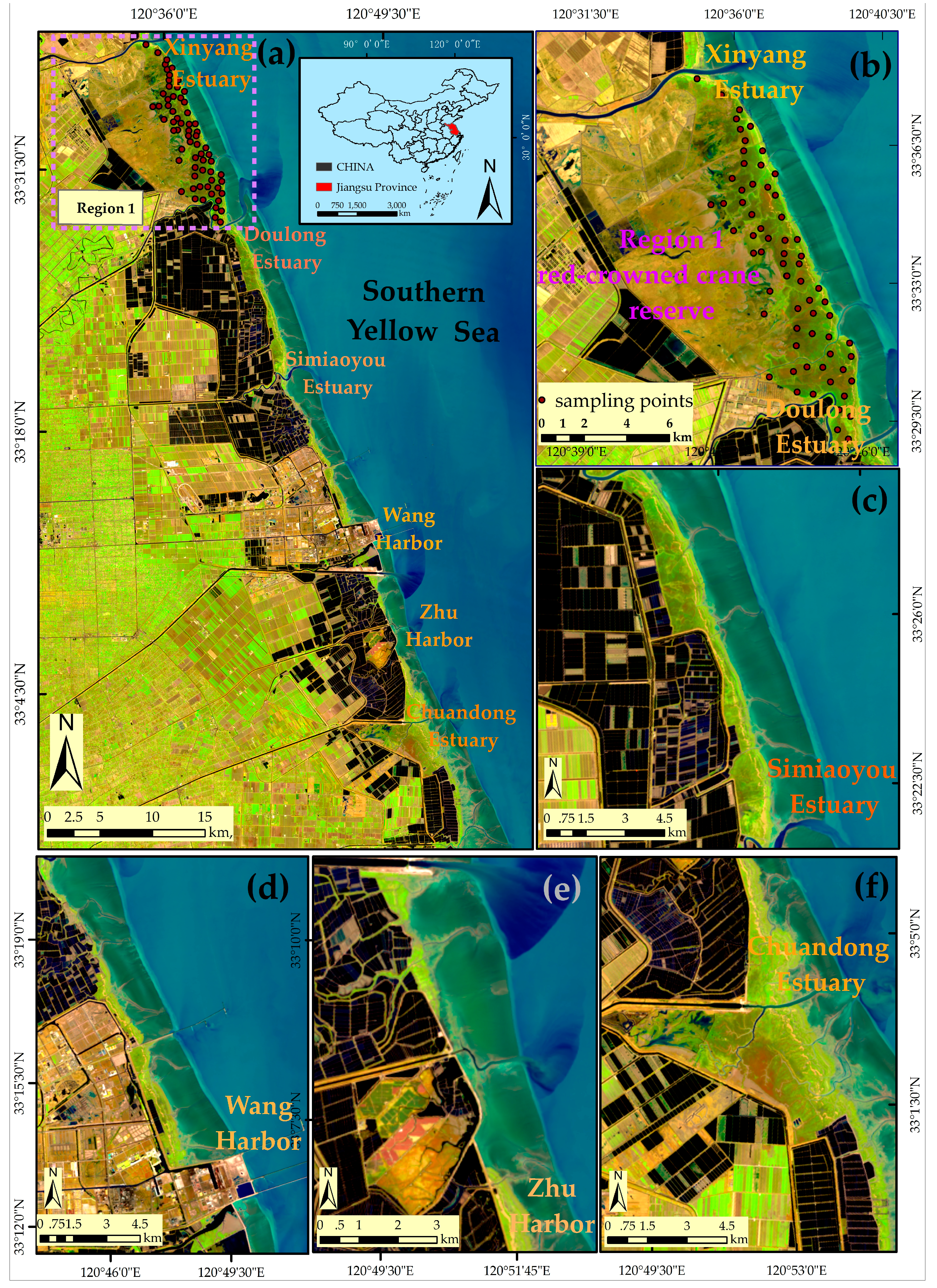
The middle coast of Jiangsu ranges from the Xinyang Estuary in the north to the Chuandong Estuary in the south (33°00′–33°40′N, 120°26′–120°55′E,). The region is located in the northern subtropical-temperate zone and has a marine monsoon climate with moderately well-defined seasonality. The coast is of the typical muddy-silt type and is occupied by native salt marsh communities, including Phragmites australis (P. australis) and Suaeda salsa (S. salsa) [9]. The non-native species S. alterniflora was introduced for the purposes of beach protection and siltation promotion in 1979 [7]. After the 1980s, the rapid expansion of the invasive species resulted in continuous changes in the species composition of the saltmarshes and threatened coastal environments [14], for example clogging navigation and flood control channels [7], reducing the open mud feeding habitats of shorebirds [4], competing with native plants [12] and even decreasing biodiversity [16]. It is therefore urgent to assess in detail the distribution of S. alterniflora for the purposes of invasion control and biodiversity conservation.
Currently, the various salt marsh communities are mainly located in Region 1 (i.e., the red-crowned crane reserve, Figure 1b). The red-crowned crane reserve (33°25′0′′–33°39′04′′N, 120°26′40′′–120°40′40′′E, Figure 1b) totals approximately 19,100 ha. In 2009, the remaining natural wetland in Region 1 accounted for only 11% of the total area, facing increasing pressure of further loss, degradation and fragmentation due to the land conversion and invasion of S. alterniflora [14]. Here, we chose Region 1 as a training area for the development of an efficient method for S. alterniflora detection and then tested the suitability of the method for application to the whole region (Figure 1a).
2.2. Remote Sensing Data
The study site is covered by a Landsat footprint (Path 119, Row 37) (Figure 1). A total of 46 Landsat images was acquired, but only 16 Landsat images had less than 10% cloud cover over the study area in 2014. Due to the cloud contamination, no Landsat image was free of clouds and of good quality (< 10% cloud cover) in August in 2014. The cloud-free image acquired in August in 2013 was used as alternative. Given the acquisition time of these Landsat images, 6 Landsat 8 OLI images and 6 Landsat 7 ETM+ images were selected for the monthly time-series analysis (Table 1). All the Landsat images were freely downloaded from USGS [69].
The pre-processing of Landsat images mainly includes geometric correction, strip noise removal, image cropping and feature extraction. Atmospheric correction of the Landsat TM image was performed by using the Fast Line-of Sight Atmospheric Analysis of Spectral Hypercubes (FLAASH) software package in Environment for Visualizing Images (ENVI). Additionally, we generated NDVI, Enhanced Vegetation Index (EVI), Ratio Vegetation Index (RVI) and Difference Vegetation Index (DVI) (see Table 2 for full names and definitions) from each image that were commonly used for estimating vegetation and land cover features. For Landsat data, some of the original bands may be highly correlated; to save data storage space and computing time, such bands could be transformed into new, less correlated bands by PCA [70,71]. Tasseled Cap Transformation (TCT) was originally developed for understanding changes in crop development and has recently also proven useful for time-series analysis [29,72]. In this study, PCA and TCT were conducted monthly on the Landsat data, and then the first three principal components of PCA (PC1, PC2 and PC3) and three orthogonal bands of TCT (TC1, TC2 and TC3) were selected as predictive variables for the time-series analysis.
2.3. Reference Data
Two field trips in Region 1 (Figure 1b) were conducted in July and September 2014 to collect ground reference samples. With a handheld GPS unit, we recorded the location of S. alterniflora, native species and other land cover types. In total, 274 S. alterniflora points, 71 P. australis points, 63 S. salsa points and 128 other land cover type points were collected as testing samples. Due to the difficulty in collecting sufficient ground truth samples at the Landsat scale, the reference data for evaluating the efficacy of the detection strategies was also obtained through the classified Google Earth (GE) image [73]. The GE image, acquired on 27 April 2014, was originally taken from the QuickBird imagery and has red, green and blue bands with a high spatial resolution, which can be downloaded from the software of LocaSpace Viewer [74]. The detailed spatial information offered by the image can help accurately distinguish S. alterniflora from other land cover types. Figure S1 illustrates the step-by-step process of interpreting the training samples and validation samples in Region 1:
Firstly, the GE image was classified using the visual interpretation method. Eight classes were classified in our classification map, and the overall accuracy of the classification result calculated from the field samples was 93.81% and the Kappa coefficient was 0.91. For recognizing S. alterniflora, the User’s Accuracy (UA) and Producer’s Accuracy (PA) were 96.15% and 95.99%, respectively (Table S1).
Secondly, the classification result was spatially resampled to 30 m to match the resolution of the Landsat imagery. The land cover type of each resampled pixel was determined when the fraction of the main land cover type was greater than 50% within the corresponding 30 m × 30 m pixel-block in the original classification result [17].
Thirdly, according to the classification result, 500 presence points and 1500 absence points were randomly generated. Then, the presence point data were divided into training and testing data. In order to reduce the influence of un-scanned gaps in the ETM+ SLC-off imagery on detecting S. alterniflora, the training and testing data for assessing the strategies of detection should not be sampled from the SLC-off gapped area [17].
Finally, after removing the points located in the SLC-off gapped area, 66 presence points (Figure 1b) were used for training the model, while the other 346 presence points and 1019 absence points were reserved for testing.
3. Methods
3.1. Biased Support Vector Machine
For comparison purposes, the Biased Support Vector Machine (BSVM) [44] was also employed to classify the same dataset with Maxent. BSVM was implemented with a radial basis kernel and thus required the optimization of three parameters: inverse kernel width σ, the weights of negative errors c, and the factor j representing the bias of weight between positive errors and negative errors. The performance of BSVM critically depends on suitable parameter values. Parameter or model selection is done by optimizing a performance criterion PCm, m = 1, …, M, over M candidate models differing by combinations of the parameters {c, j, σ} m [51]. In the case of BSVM, zero or the separating hyperplane is considered as a “natural” threshold. We also consider the Equal Training Sensitivity and Specificity (ETSS) as a threshold [62] that can be derived easily for BSVM. Then the accuracies for the two thresholds were calculated by using independent test data, and the results of the best threshold were used. Finally, we compared the performances of the proposed OCC approaches of Maxent and BSVM under the 15 schemes of Experimental Setups 1–3 (Section 3.3).
3.2. Maxent Model and Tuning of Complexity
As a general-purpose machine learning method, the Maximum entropy (Maxent) approach [56,57,75] is also suitable for mapping real distributions based on remote sensing data [29,36,45,51,52,53,55,58,59,60,62]. Maxent is available free for educational and noncommercial use as a multi-platform Java-based software [76]). Model complexity, defined as the number of parameters included in a model, is typically constrained via a process known as L1 regularization [66]. The complexity of Maxent models can be adjusted by the settings of the Regularization Multiplier (RM) and Feature Combination (FC) [57,66,72]. First, in order to find the correct level of model complexity, we built models with RM values ranging from 0.5–4.0 (in increments of 0.5) and with six different FC combinations (L, LQ, H, LQH, LQHP, LQHPT; where L = Linear, Q = Quadratic, H = Hinge, P = Product and T = Threshold), which was implemented in the R package ENMeval [66]. This process was performed iteratively until each locality was used to test the model once and was repeated for each different combinations of feature classes and regularization multipliers. The resulting models were evaluated using AICc [67], and the model parameters that resulted in the lowest AICc value (i.e., △AICc = 0) were chosen for each. Then, the model complexity was evaluated by comparing the relative performance of Maxent-DPS (RM = 1, FC = LQH) models with Maxent-AICc models by the independent test data.
In the case of Maxent, there is no fully automatic method available for selecting an optimal threshold. Usually, one out of a few considered candidate thresholds reported by the software is used based on subjective user decisions or by using positive and negative reference data [53]. Here, we selected the equal training sensitivity and specificity (ETSS) as the threshold [62]. The models from Experimental Setups 1–4 were all developed with the same occurrence (66 random points), 10-fold cross-validation and the prevalence of 0.5. Other parameters not mentioned here were set as the default. In training area, the background data of 10,000 random points in different models (Experimental Setups 1–3, Section 3.3) were all randomly extracted from the entire area (Figure 1b) [77]. In the larger area, the background data (10,000 random points) was extracted from the entire study area (Figure 1a).
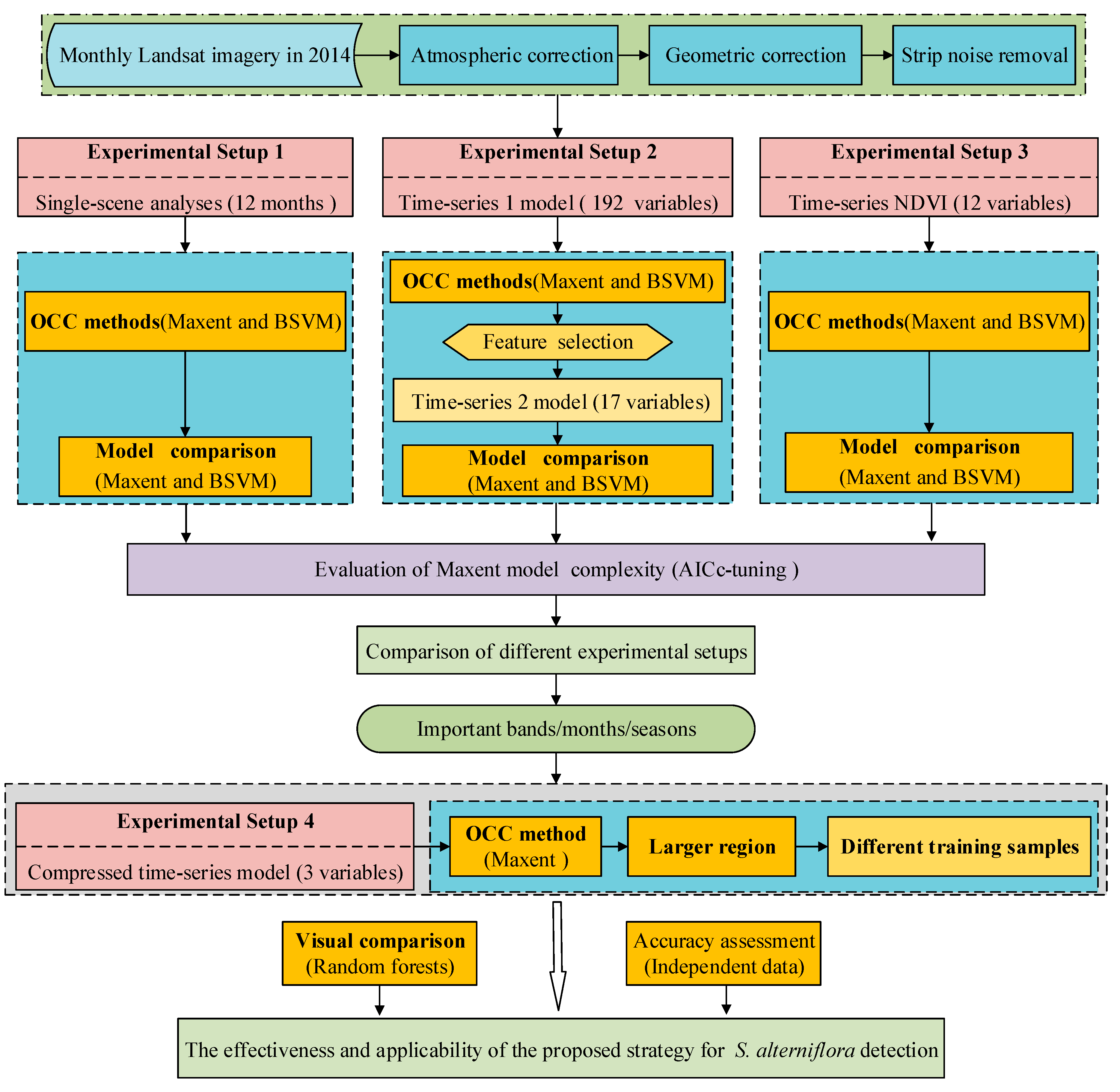
3.3. Four Experimental Setups
As shown in Figure 2, four experimental setups were developed from the monthly Landsat time-series data. These setups are as follows:
Experimental Setup 1 was mainly used for the comparison between two OCC methods (Maxent and BSVM) and the assessment of their discrimination abilities in different months. There were 12 single-scene analyses in Setup 1: each model used six bands, blue, green, red, NIR, SWIR1, SWIR2, the four vegetation indices (NDVI, DVI, RVI, EVI), the first three components (TC1, TC2, TC3) after the tasseled cap transformations and the first three components after principal component analysis (PC1, PC2, PC3).
Experimental Setup 2 was implemented to evaluate the performance of the time-series analysis, along with the selection of important band variables and phenological stages in detecting S. alterniflora. Two time-series models were built in Setup 2: the first Time-Series model (TS-1) and the second time-series model (TS-2).
One hundred and ninety-two predictor variables, generated from the 12 single-scene analyses, were used in the TS-1 model. The TS-2 model was conducted using three procedures. First, we restricted the Maxent model to the variables that had a permutation importance value >0% (n = 75) and used them as predictor variables. The 75 variables were then tested for correlations using ENMTools_1.4.4 [78]. For variables that were highly correlated (Pearson correlation coefficient >0.80), we removed those that had the least predictive contribution in the TS-1 model [29]. This further reduced the number of variables to 24 potential predictor variables. Second, we operated the Maxent model by using the selected 24 predictor variables. Third, according to the results output from the model in the second procedure, we selected the variables with a permutation importance value >0%. This finally reduced our number of variables to 17 potential predictor variables for our second time-series model (TS-2). Both Maxent and BSVM methods were used to operate the TS-1 and TS-2 models.
Experimental Setup 3 was created to evaluate the performance of the time-series analysis with monthly NDVI and to investigate the role of NDVI in detecting S. alterniflora. The Time-Series NDVI (TS-NDVI) model was conducted using 12 NDVI indices from 12 months (January–December NDVI). Both Maxent and BSVM methods were used to build the TS-NDVI model.
Experimental Setup 4 was developed to verify the expansibility of the proposed detection strategy over a larger region. Firstly, to make the strategy simpler and easier to apply, the top three band variables (December NDVI, March green and January PC3) from the TS-2 model were selected to build a compressed time-series model. Secondly, the performance of the compressed time-series model was tested in the training area (Figure 1b). Thirdly, the three variables were rebuilt to match the entire study area. Finally, the Maxent model was rebuilt by using these reconstructed variables over a larger region.
3.4. Evaluation of the Expansibility of the Method and Settings of the Training Sample Size
In order to verify the expansibility of the proposed detection strategy, we applied the method to a larger region (Figure 1a). In addition, we also investigated the possible impacts of training sample size on the performance of S. alterniflora detection in the region. Figure 3 illustrates the procedure to generate the reference dataset and the final land cover map in the larger region.
3.4.1. Reference Dataset and 70 “Sets” of Training Samples
As shown in Figure 3a, first, 2678 samples were randomly created based on the Landsat image (30 m). Second, the 2678 sample points were overlaid with the Google Earth high-resolution base map and manually classified as presence points (S. alterniflora: 830 points) or as absence points (non-S. alterniflora (seven classes): 1848 points) using a visual interpretation; this further generated our reference dataset. Third, 150 presence points were selected as training samples from the reference dataset, and then, different “sets” of training samples: 10, 20, 30, 40, …, 140 (at an interval of 10) points were randomly extracted from the 150 sample points. This process was repeated 5 times. Thus, 70 “sets “of training samples in total were obtained. Finally, we applied the Maxent model using three variables (See Section 3.3) in the region and evaluated the performance based on validation samples.
3.4.2. Final Land Cover Map
For visual comparison purposes, the land cover classification map of this region was created with a random forests algorithm (see Appendix A) using 17 variables. As shown in Figure 3b, first, the reference dataset (eight classes, 2678 sample points) was randomly divided into training samples (1339 points) and validation samples (1339 points). Second, the parameters of the RF algorithm were tuned to obtain the optimal prediction accuracy (see Appendix A for details). Third, the initial land cover classification map was created using the RF algorithm with the optimum parameter combination (mtry = 3, ntree = 1500, Figure A1). Finally, the initial land cover classification map (with a Kappa of 0.79 and an OA of 83.05%, Table A1) was modified by referring to the classification map reported by Sun et al. [14] and GE imagery in this region; this further generated our final land cover classification map (Figure S2).
3.5. Model Verification
The confusion matrix was constructed for each classification strategy with the testing samples to evaluate the model performance. Several accuracy indices were calculated from the confusion matrix: Overall Accuracy (OA), the Kappa statistic, specificity and sensitivity, which were done in the R environment using the SDMTools packages [79]. Sensitivity, also called the true positive rate, measures the proportion of positives that are correctly identified. Specificity, also called the true negative rate, measures the proportion of negatives that are correctly identified [79]. A paired samples t-test was performed to compare the results statistically and look for any significant differentiations.
Since these accuracy statements were derived from the same training samples, we used McNemar’s test to assess the statistical significance of differences in classification accuracy [17,80]. It is a non-parametric test for evaluating the statistical significance of the difference between two classification results based on the same testing samples. McNemar’s test is based on the chi-square test statistic and computed as follows:
where f12 denotes the number of testing samples correctly classified by the first classifier, but incorrectly classified by the second classifier. Similarly, f21 denotes the number of testing samples correctly classified by the second classifier, but incorrectly classified by the first classifier. Two classifications differ at the 95% level of confidence if |X| > 1.96 [47,80].
4. Results
4.1. Model Comparison
We compared the relative performance of Maxent and BSVM in Experimental Setups 1–3. As shown in Table 3, the OA and Kappa of Maxent were 80.37–95.46% and 0.49–0.88, respectively, while the OA and Kappa of BSVM were 79.49–95.89% and 0.43–0.89, respectively. It was found that the average values of OA and Kappa of Maxent were higher than those of BSVM (Table 4). Moreover, Maxent yielded a higher average value of sensitivity and specificity than did BSVM (Table 4). Combined with the result from the visual comparison (Figure A2), BSVM tended to produce a slightly higher omission rate for the prediction of S. alterniflora.
For most of the schemes of Setups 1–3, McNemar’s chi-square test rejected the null hypothesis that the error rates for these two strategies were the same (p < 0.01, Table 3). We also used paired samples t-test techniques to compare the mean differences in the accuracy value (i.e., OA, Kappa, specificity, sensitivity, omission) derived from the two methods. The result showed that there was no statistical difference between the two classifications based on Experimental Setups 1–3 at a confidence level of 95%, which indicated that Maxent and BSVM performed similarly.
However, for those months in summer, Maxent produced higher OA and Kappa values than BSVM (Table 3), which suggested that Maxent appeared to have a more balanced performance than BSVM over the summer months (Table 3). Moreover, Maxent was easier to operate in a software environment and directly provided the variable importance together with the results; however, a separate calculation has to be done for the BSVM. Given the advantages and more stable performance achieved, Maxent was mainly used for subsequent exploration of the crucial phenological stages (Section 4.3), the role of the optimal bands in recognizing S. alterniflora (Section 4.4) and evaluating the suitability of the method for application to a larger region (Section 4.5).
4.2. Model Complexity Analysis
We compared the relative performance of the Maxent-DPS and Maxent-AICc models. The Maxent-AICc model was significantly different from Maxent-DPS: the Maxent-AICc models had higher RM values than the Maxent-DPS models of 1.0 (Table 5). Since a higher regularization multiplier can smooth response curves by imposing a higher penalty for the inclusion of parameters [66], this result suggested that the Maxent-DPS model tended to result in more complex models relative to the Maxent-AICc model.
Figure 4 shows that the Kappa and OA of the Maxent-DPS models generally were slightly higher than the Maxent-AICc models; however, the Kappa and OA of the Maxent-DPS models were slightly lower than the Maxent-AICc models in Experimental Setup 2 (TS-1 and TS-2). The different performances of the Maxent-DPS and Maxent-AICc models in Experimental Setups 1–3 showed that model complexity had an impact on the performance of the model, especially when many variables were used. Moreover, compared with Maxent-DPS models, as shown in Table 6, the Maxent-AICc model had a higher sensitivity (the average of sensitivity of Maxent-DPS was 0.007 higher than that of the Maxent-AICc model), indicating lower omission rates for the S. alterniflora prediction and less overfitting. However, the Maxent-AICc model also showed much lower specificity, suggesting that they tended to over-predict the actual distribution of the S. alterniflora.
Based on the result from the paired-samples t-test, there was no statistical difference between the Maxent-DPS and Maxent-AICc models at the confidence level of 95% (Table 6), which, in other words, indicated that the discrimination power of the Maxent-AICc model was not significantly weaker than that of the Maxent-DPS model. Therefore, the Maxent-AICc model was used for subsequently selecting the crucial phenological stages (Section 4.3) and optimal bands in recognizing S. alterniflora (Section 4.4).
4.3. Important Months and Seasons in S. alterniflora Detection
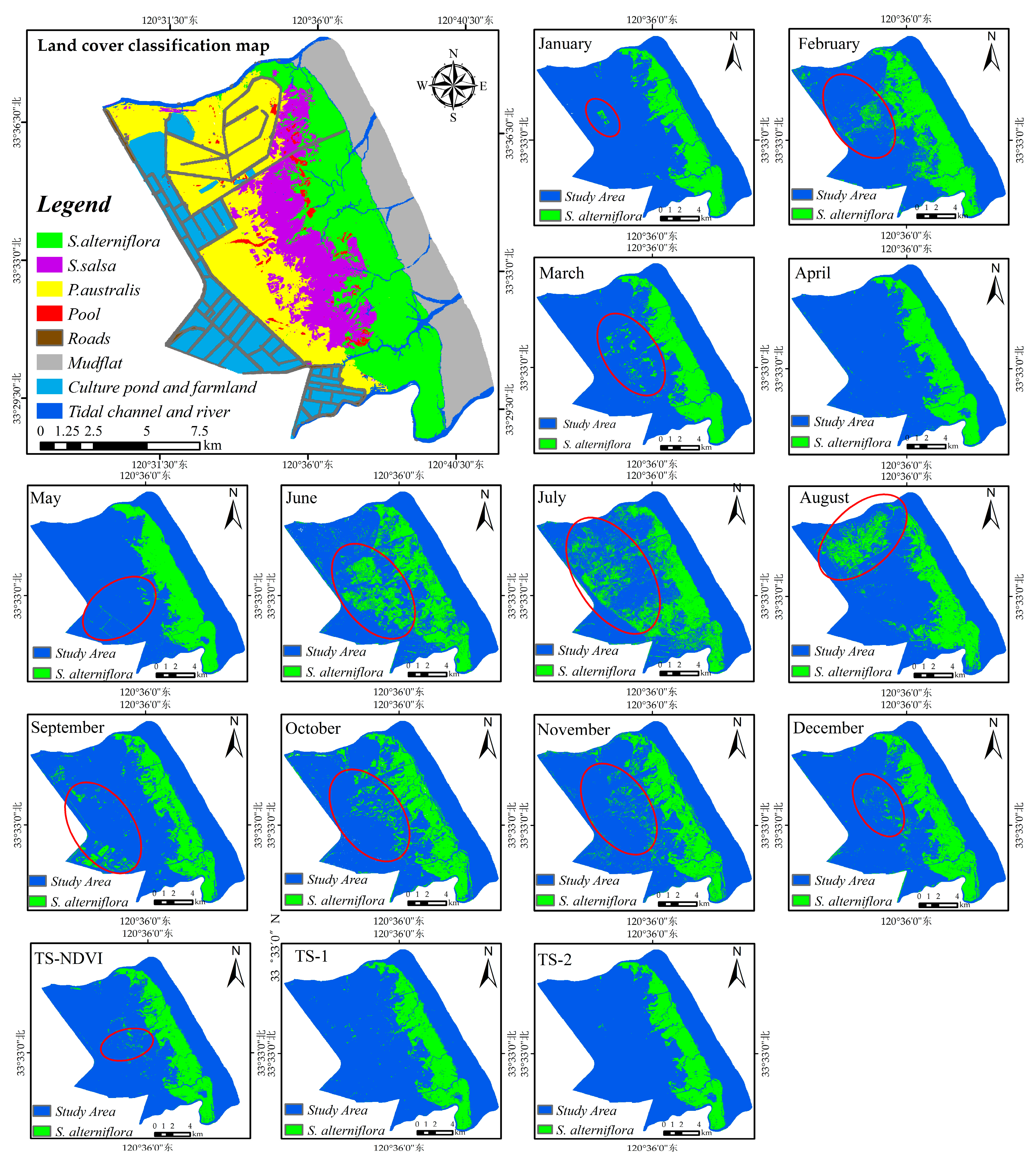
As shown in Figure 5, in Experimental Setup 1, most single-scene models generally performed well except for the June, July and August single-scene models, further highlighting the applicability of the Maxent OCC approach with remote sensing for detecting S. alterniflora. The best model was the April single-scene analysis with an OA of 94.36 and a Kappa of 0.84. In general, spring (March–May) was the best season for recognizing S. alterniflora by using the Maxent OCC approach: S. alterniflora spectral signatures were obviously different from all other land covers (Figure 6). The Kappa and OA of this season were above average (Figure 5), and the boundaries of S. alterniflora were clear, except for a small number of native vegetation patches that were incorrectly divided into S. alterniflora in March (Figure 7). The next best season for recognizing S. alterniflora was autumn (September–November): the Kappa and OA fluctuated between average levels and the misclassification patches were slightly increased. In addition, the performance in early and middle winter (December, January) was higher than it was in autumn, but the performance in late winter (February) was much poorer. The worst season for recognizing S. alterniflora was summer (June–August), with a lower value of Kappa and OA, and the number of misclassification patches increased significantly (Figure 7). In this season, S. alterniflora exhibited similar spectral reflectance signatures as other saltmarsh plants (Figure 6).
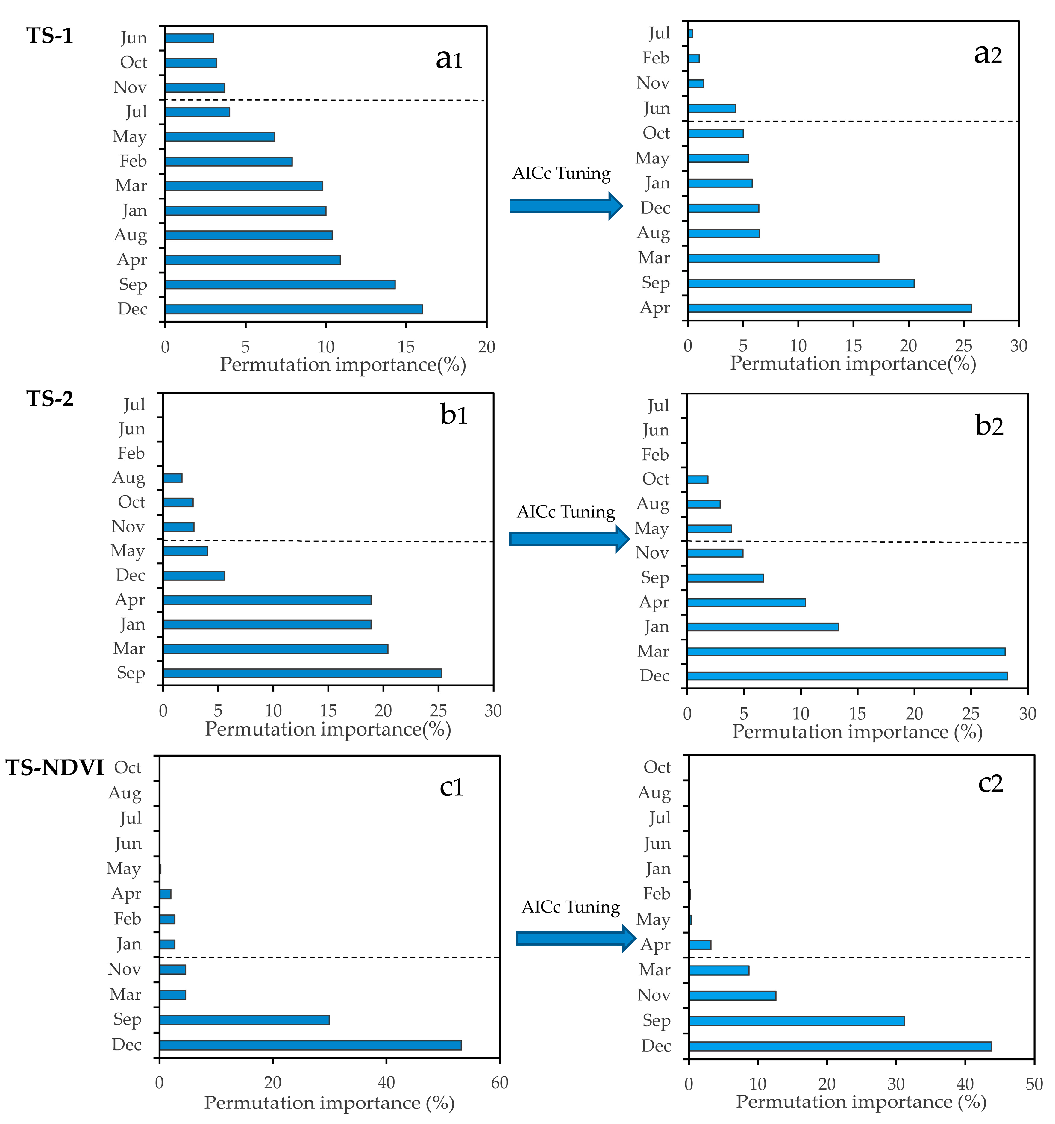
Our results suggested that the time-series analyses demonstrated a higher discrimination ability between S. alterniflora and native plants than a single-scene analysis (Figure 5 and Figure 7). Particularly, for the second time-series model (TS-2), the overall accuracy was approximately 1.10% higher than for the April single-scene model, and there was an increase of 0.034 in the Kappa coefficient. However, as for the TS-NDVI model, the model performance was not significantly improved. In the TS-1 model, the cumulative permutation importance of ten months exceeded 90% of the total (Figure 8a). However, as for the TS-NDVI model, the model performance was not significantly improved. In the TS-1 model, the cumulative permutation importance of eight months exceeded 90% of the total. However, some of these months (e.g., August, October) showed poor performances in Experiment Setup 1, but had high permutation importance (Figure 5 and Figure 8a), which suggested that the TS-1 model had a low ability for selecting important feature variables. In the TS-2 model, the cumulative permutation importance of six months (January, March, April, September, November, December) exceeded 90% of the total (Figure 8b), and the six months in Pattern 1 performed well with high accuracy (Figure 5), which indicated that the TS-2 model after feature selection (see Section 3.3) was more conducive to revealing the critical time window in detecting S. alterniflora. In addition, in the TS-NDVI model, four months (March, September, November, December) exceeded 90% of the total (Figure 8c). The result showed that the time-series analysis with monthly NDVI was slightly different from that with the multi-band combination, especially for the importance of the spring months.
4.4. Important Band Variables and Their Roles in S. alterniflora Detection
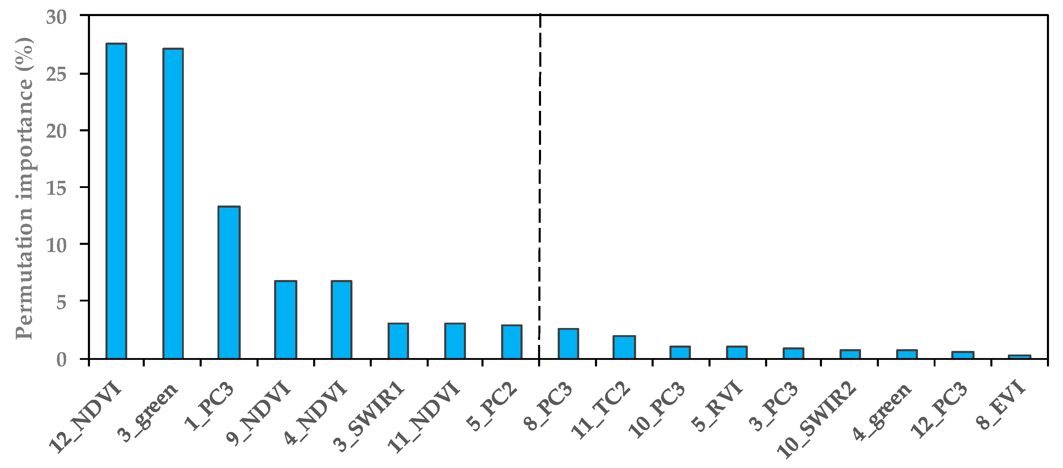
In Experiment Setup 1, as shown in Table 7, each single-scene analysis had at least one TCT, PCA or VI as one of the top three predictors. Moreover, TCT, PCA and VI accounted for approximately 13 of the 17 variables of the TS-2 model (Figure 9), which indicated that the methods of spectral enhancement and the vegetation index can effectively improve the ability in detecting S. alterniflora.
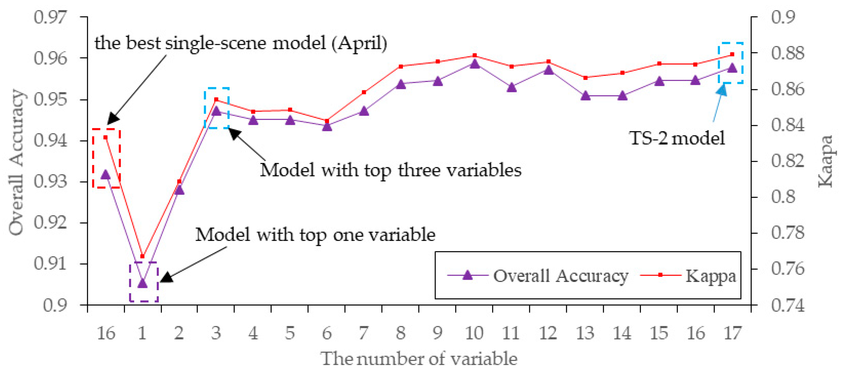
As shown in Figure 9, the top three predictors for the TS-2 model were the December NDVI (27.6%), March green (27.1%) and January PC3 (13.3%). The total importance value of these bands’ variables exceeded 68%. Therefore, we investigated the roles of these optimal bands’ variables by testing the model performances by adjusting the number of variables from 1–17 (Figure 10). The Maxent model, using only the top one band, yielded an OA of 90.66% and a Kappa of 0.75, which were higher than those of seven single-scene models in Experiment Setup 1 (Figure 6 and Figure 10); and when using the top three variables to create a model, the OA and Kappa were higher than those of the best single-scene analysis (Figure 10). This indicated that the time-series analyses can better distinguish the phenological differences between S. alterniflora and native plants than a single-scene analysis.
4.5. Applicability of the Method for S. alterniflora Detection in Large Regions
We applied the Maxent model with compressed time-series (i.e., Maxent using only three band variables) to a larger region and investigated the possible impacts of the number of training samples. As shown in Figure 11, it was amazing that the overall results produced consistently high mapping accuracies under different training sample sizes, with >0.85 OA and >0.71 Kappa. Moreover, for S. alterniflora detection, the best classification accuracy was achieved with 70 training samples rather than with more samples used. The results indicated the strong ability of Maxent to deal with a small sample.
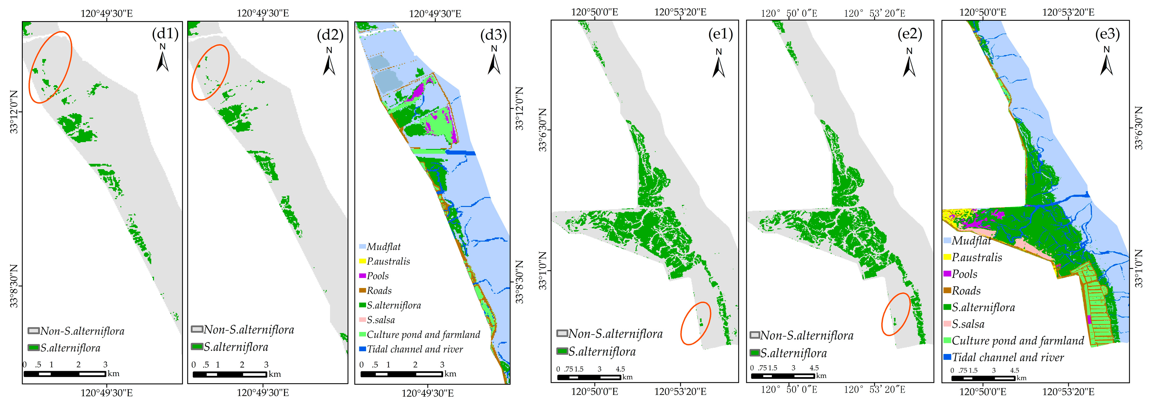
Figure 12 shows the classification performance of the model using the number of training samples of 10 and 70. The visual comparison showed that for recognizing S. alterniflora, the performance of the model using 10 and 70 samples was rather similar. As for the model using 70 samples, although there were a few misclassification errors, especially in the red-crowned crane reserve (Figure 12(a2)), our classification result is consistent with the result from final land cover classification map (see Section 3.4 for details), regardless of the overall distribution or local details. In addition, our result agrees well with the classification results reported by Sun et al. (2016) [14]. Therefore, the performance of the method is generally stable and will be appropriate for large-scale S. alterniflora detection.
5. Discussion
5.1. Performance of OCC Methods for S. alterniflora Detection and Model Complexity Analysis
Both Maxent and BSVM methods successfully identified S. alterniflora with good accuracies, further highlighting the applicability of OCC methods for detecting invasive species. Compared with BSVM, Maxent appeared to have a more balanced performance over the summer months. Although a large number of studies has reported that Maxent has a great advantage over other OCC methods based on remote sensing data, model complexity was completely ignored in most cases [13,29,36,45,46,51,55,58,59,62]. Only a few studies have taken into account the problem of model complexity in remote sensing mapping [81,82]. The main reason for the above phenomenon is that the tuning of model complexity is prohibitively laborious and time consuming [66], and the current Maxent-DPS can result in good performance in most cases [57]. Our results showed that S. alterniflora can be accurately distinguished using the Maxent-DPS model. However, the results also indicated that Maxent-DPS tended to result in more complex models relative to Maxent-AICc models, and not all the models with Maxent-DPS showed a higher performance than that of Maxent-AICc models. Despite this fact, complex models generally showed slightly better performance in mapping current distributions in the study, but they may produce poor predictions in some cases.
Based on the result from the paired samples t-test, the Maxent-AICc model was found not to be weaker than the Maxent-DPS model. Moreover, the AICc procedure produced models that outperformed the Maxent-DPS model in selecting the true relative importance of variables for detecting species. These findings agreed well with previous reports [61,63]. As shown in Figure A3, the order of month importance of the AICc selected models were different from that of the Maxent-DPS models over three time-series analyses. As for the TS-1 analysis, in Maxent-DPS model, some months (e.g., February, June, July) showed poor performance for the S. alterniflora detection, but had high permutation importance values, while the values of these months in the Maxent-AICc model were much lower. As for the TS-2 analysis, in the Maxent-DPS model, September was the most important month, while December was the top one month in the Maxent-AICc model. The result showed that in the single-scene analysis, the performance in recognizing S. alterniflora in December was better than that in September. As for the TS-NDVI analysis, the Maxent-DPS model and the Maxent-AICc model performed equally well for the selection of crucial phenological stages. Therefore, the result indicated that the Maxent-AICc model appeared to have a better performance in selecting important phenological stages for S. alterniflora detection. Given the good performance of the Maxent-AICc model, we thus suggest that model complexity should be considered in the field of remote sensing, and tuning regularization with AICc will help address this issue.
5.2. Important Phenological Windows and the Role of NDVI for S. alterniflora Detection
In this study, December and April were found to be the crucial phenological windows for recognizing S. alterniflora. This finding agrees well with the results from Ai et al. (2017) [21]. In April, the native salt marshes are germinating or growing, while most of S. alterniflora remains dormant [14]; in December, S. alterniflora can preserve more green vegetative parts [25], while most native salt marshes are in complete dormancy due to the phenology of S. alterniflora lagging behind the native salt marshes in the study area. These phenological phenomena can result in statistical spectral differences between S. alterniflora and the native marshes.
Besides the two important phenological windows, we found that the bands in September, March and May also have played important roles in our time-series analyses. Usually, in early September, the bloom of S. alterniflora changes its pigment content, proportion and canopy structure, while P. australis is in a vegetative growth or inflorescence stage and S. salsa is in a withering stage [25]. In late March and early May, the native marshes S. salsa and P. australis are germinating or growing, while most of S. alterniflora remained dormant. Since S. alterniflora is widely distributed along the coast wetlands with significant latitudinal differences, the timing of plant phenology also varies considerably within a single remote sensing image. Although comparable results may be achieved by using single-scene images in those optimal phenological stages, the actual result may be extremely sensitive to the choice of the remote sensing image if the method were applied to a larger region. Therefore, these phenological stages (i.e., September, March and May) should be considered, although spectral differences between invasive species and native species in these months were not as big as those in the optimal time window (i.e., April and December).
Compared with contiguous and narrow bands of hyper-spectral sensors, Landsat imagery contains some broad bands that may mask small and local phenological variations [25], which may result in poor separability between S. alterniflora and native salt marsh. We found that specific Vis (e.g., NDVI, RVI, EVI) and spectral enhancement methods (e.g., PCA and TCT transformations) can help increase the potential to discriminate between vegetation species. It was noted that NDVI (September, December, April, November) played an important role in the TS-2 model with high permutation importance (44% in total). NDVI is an effective measure for separating vegetated areas from non-vegetated regions [83,84], and its great potential for distinguishing various salt marshes has been proven with some studies [14,85,86]. Our results also indicated that NDVI, especially in the optimal phonological window (i.e., December), was an important index for S. alterniflora detection.
Recently, for mapping the distribution of S. alterniflora, Sun et al. (2016) [14] have proposed a time-series NDVI analysis strategy based on a multi-class classification method and have obtained high accuracy. In our study, the time-series NDVI analysis with the OCC method produced relatively higher accuracy than most single-scene analyses. However, our results also showed that the performance of the NDVI time-series model was poorer than other time-series models, even the time-series models with only three band variables. Compared to other time-series models, the decreased performance using time-series NDVI may be caused by the reduction of critical information on the land cover obtained in each month. Additionally, since S. alterniflora often grows in intertidal zones and is often impacted by tidal fluctuations, more noise will be introduced if more images are involved [87]. The effects of spatiotemporally heterogeneous conditions may accumulate in the time-series and interfere with S. alterniflora detection [14]. Therefore, for the NDVI time-series analysis, it is critically important to pick out a few images that best reflect the differences between various species and thereby reduce the span of the NDVI time-series. Given the encouraging results from the compressed time-series analysis, we suggest that time-series analysis using critical phenological NDVI and multispectral bands may be more efficient for S. alterniflora detection rather than only the composite NDVI bands.
5.3. Opportunities and Challenges for S. alterniflora Detection Using the Phenology-Based OCC Approach
Our results demonstrated that the phenological time-series analysis with the OCC method was also suitable for S. alterniflora detection over a larger region. The promising results achieved by the model in the region indicated its robustness and potential for large-scale application, which is crucially needed for S. alterniflora studies and management. Previous studies have proven that Maxent is applicable to presence-only data and has good performance in recognizing invasive species even with low sample sizes [52,58], which may reduce the requirement for training data collection [58]. Our classification results were consistent with their findings. In light of the good results of the proposed method, we believe that our Maxent OCC method combined with time-series analysis can be extended to geographical areas that share similar species composition and will enhance our ability to detect S. alterniflora and other invasive plant species.
Despite promising results, there are still several limitations and uncertainties of the proposed method that need to be considered before it is employed for large-scale S. alterniflora monitoring. First of all, GE imagery, as a freely available data source, has great advantages for recognizing S. alterniflora, especially for discerning small, newly-colonizing S. alterniflora clumps at an early stage [26]. Therefore, in the study, for evaluating the expansibility of the proposed method over a larger region, both training and test samples were built based on the GE image. These samples were generated with careful visual interpretation of the GE imagery and referenced against the classification results of Sun et al. (2016) [14]. The selected samples were thus appropriate, but may not be the most optimal. The accuracy of the samples need further examination due to the lack of ground truth data.
Second, the classification efficiency of time-series is highly correlated with the stability of the plants during the study period [87]. The annual variation of the species niche hinders the accurate mapping of salt marsh vegetation, especially for the ecotones and boundaries of different salt marsh communities [14], which are areas of high misclassification probability, complicating their accurate distinction. Therefore, in future studies, it is necessary to collect high quality reference data that contain different months for these sensitive regions to formulate a more stable and generalized time-series detection model.
Last, for larger-scale S. alterniflora detection, it is sometimes difficult to acquire sufficient monthly cloud-free Landsat images during a year. Under these circumstances, the ESA’s Sentinel-2A and B constellation (with 10-m, 20-m and 60-m spatial resolution and a repetition cycle of five days) [88] and the Chinese HuanJing-1 (HJ-1) A/B satellite (with the spatial resolution of 30 m and a temporal resolution of two days [89,90]) can be used as important supplement data for the Landsat satellite to formulate the complete time-series analysis model. Moreover, our time-series analysis model using only the selected three band variables can obtain very high accuracy. Therefore, despite the limitations in acquiring sufficient monthly cloud-free images, we can pinpoint several months that capture the key phenological differences between plants, which may help to improve classification performance. In this case, we can use the MODIS vegetation phenology products (e.g., green-up products) from the U.S. Geological Survey to guide the selection of images of key phenological stages. To this end, further improvements to our methods are needed to formulate a more robust spatially generalized detection model by employing different sensors across multiple spatial scales and diverse geographical regions.
6. Conclusions
Mapping the distribution of S. alterniflora is urgently needed to evaluate the ecological effects of the invasive species on wetland ecosystems. However, it is still challenging to map S. alterniflora in a coastal wetland environment. In this study, we applied OCC methods based on Landsat time-series imagery to detect the species. To develop a new phenology-based strategy to detect the species, we first conducted four experimental setups. Based on Experimental Setups 1–3, we found that Maxent and BSVM performed equally well, and Maxent appeared to have a more balanced performance over the summer months. Compared with the Maxent-AICc model, Maxent-DPS tended to result in more complex models; we thus suggested that the model complexity of Maxent should be considered and can be tuned using the AICc procedure.
Compared with single-scene analyses, time-series analyses can better distinguish phenological differences between S. alterniflora and native plants. Moreover, we found that two optimal phenological windows are important for S. alterniflora detection: the senescence stage (December) and green-up stage (April). Besides, several other months (e.g., January, March, May, September) also contributed to the detection power of S. alterniflora in time-series analysis. Furthermore, based on the time-series analyses, we found that NDVI from crucial phenological stages played an important role in recognizing S. alterniflora. Meanwhile, a compressed time-series model, including only three selected band variables (i.e., December NDVI, March green and January PC3) demonstrated higher accuracy than all the single-scene analyses. Therefore, we rebuilt the Maxent model with the optimal variable set for a larger region and found that it was also suitable for large-scale S. alterniflora detection. Given the opportunities provided by Landsat and other satellite images, we believe that the OCC method combined with a phenology-based detection strategy is appropriate for region-wide and long-term mapping of S. alterniflora.
Supplementary Materials
The following are available online at www.mdpi.com/2072-4292/9/11/1120/s1, Figure S1. The procedure to generate the reference dataset in the training area. Figure S2. Classification map for the middle coast of Jiangsu that was constructed using random forest algorithm. (a) Overview of the study area in the Landsat OLI image (R:5, G:4, B: 3) on December 29, 2014; (b) the initial land cover classification map that was constructed using random forest algorithm; (c) the final land cover classification map. Table S1. Classification accuracy assessment for the Google earth image
Acknowledgments
This research has been supported by the National Natural Science Foundation of China (Nos. 31470519, 31370484), the National Natural Science Youth Foundation of Jiangsu Province of China (Grant BK20140921) and funded by the Priority Academic Program Development of Jiangsu Higher Education Institutions.
Author Contributions
Xiang Liu formed the original idea for the study and wrote the original manuscript. Huiyu Liu offered valuable comments and suggestions for the manuscript and was responsible for manuscript revisions. Zhenshan Lin, Haibo Gong and Shicheng Lv supervised the process of data analysis.
Conflicts of Interest
The authors declare no conflict of interest.
Appendix A
Random forests models build numerous decision trees, and each tree is built using a random subset of independent variables and a random sample of the training dataset [37]. The output is the class voted by most trees [91]. The input data selected for training each of the trees are in-bag observations, and the remaining are Out-Of-Bag (OOB) observations used for estimating OOB errors [38,91]. The prediction accuracy of random forests models is evaluated by the OOB error.
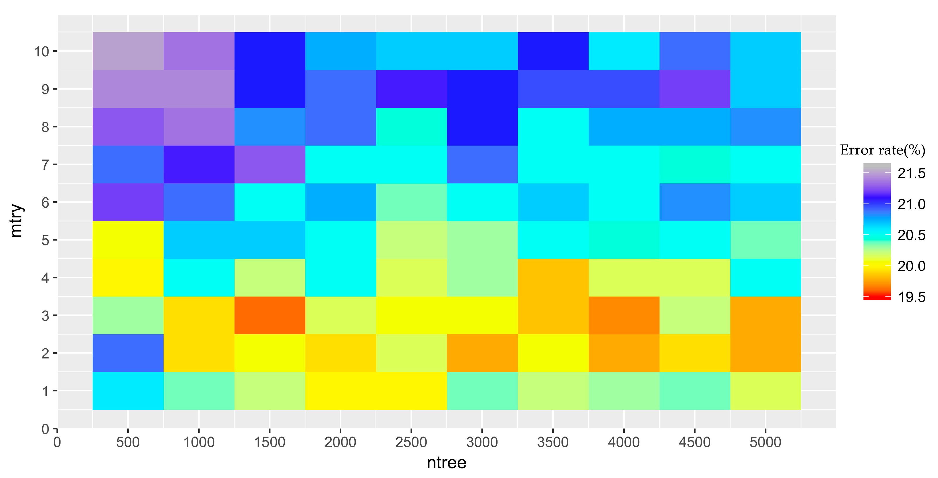
The optimization of random forests models requires two finely-tuned parameters: the number of decision trees (ntree) and the number of features randomly selected at each node (mtry) [92]. In this study, different values for ntree and mtry were tested, and the pair that yielded the lowest OOB error will be considered optimal. The candidate values for ntree were from 500–5000 with increments of 500; mtry was set to range from 1–10 with an interval of one. The classification algorithm was implemented within the randomForest package for R [37].
The lowest OBB estimate of the error rate appeared at mtry = 3 and ntree = 1500 (Figure A1). Therefore, this combination of mtry and ntree was used to conduct the initial land cover classification map within the study area.
Appendix B
Figure A1.
The matrix of the OOB estimate of the error rate with different combinations of mtry and ntree.
Figure A1.
The matrix of the OOB estimate of the error rate with different combinations of mtry and ntree.

Table A1.
Accuracy assessment for the initial land cover classification map using the random forest algorithm based on the confusion matrix method. TCR: Tidal Channel and River. CPF: Culture Pond and Farmland.
Table A1.
Accuracy assessment for the initial land cover classification map using the random forest algorithm based on the confusion matrix method. TCR: Tidal Channel and River. CPF: Culture Pond and Farmland.
| Prediction | CPF | Mudflat | P. australis | Pools | Roads | TCR | S. salsa | S. alterniflora | |
|---|---|---|---|---|---|---|---|---|---|
| Reference | |||||||||
| CPF | 192 | 0 | 3 | 3 | 11 | 1 | 0 | 7 | |
| Mudflat | 1 | 84 | 0 | 0 | 0 | 0 | 0 | 0 | |
| P. australis | 4 | 0 | 239 | 2 | 6 | 0 | 5 | 1 | |
| pools | 1 | 0 | 11 | 32 | 0 | 0 | 3 | 2 | |
| Roads | 16 | 1 | 11 | 1 | 48 | 1 | 5 | 8 | |
| TCR | 3 | 9 | 4 | 0 | 7 | 20 | 6 | 45 | |
| S. salsa | 0 | 0 | 10 | 0 | 1 | 1 | 108 | 5 | |
| S. alterniflora | 1 | 4 | 4 | 1 | 8 | 10 | 4 | 389 | |
| Overall accuracy: 83.05%; Kappa: 0.7895 | |||||||||
Figure A2.
Classification map of S. alterniflora based on BSVM under the 15 schemes in Pattern 1 (January–December). The red circle shows the misclassification errors.
Figure A2.
Classification map of S. alterniflora based on BSVM under the 15 schemes in Pattern 1 (January–December). The red circle shows the misclassification errors.
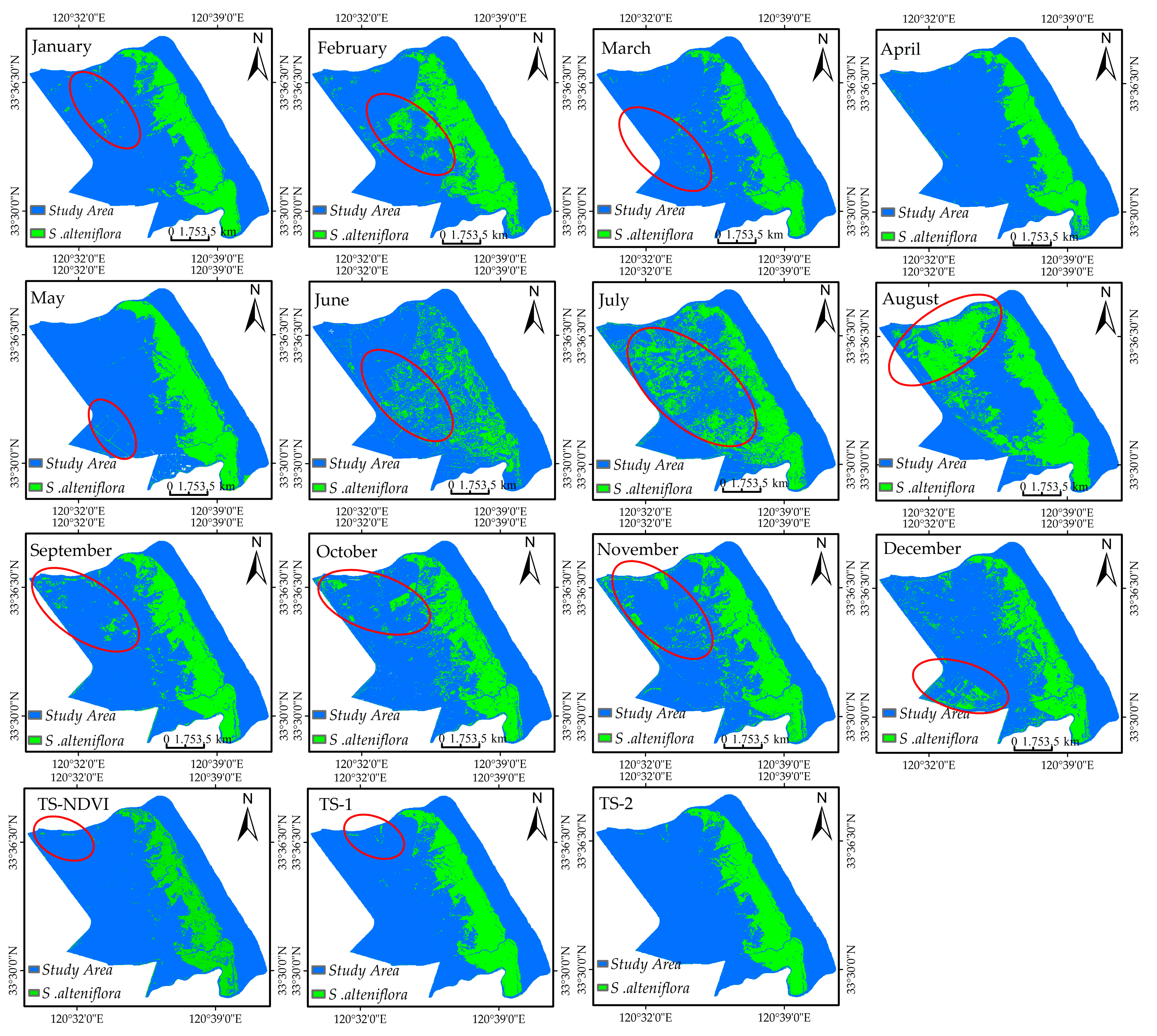
Figure A3.
Month’s importance sorted in descending order with the permutation importance value. The month importance was determined by summing the permutation importance value of all bands in each month. (a) Months’ permutation importance from the first time-series model (TS-1); (b) months’ permutation importance from the second time-series model (TS-2); (c) months’ permutation importance from the third time-series model (TS-NDVI). (a1,b1,c1) are Month’s permutation importance from three time-series models with default parameters. (a2,b2,c2) are Month’s permutation importance from three time-series models with AICc-selected parameters. The sum of the permutation importance value from the months with two time-series models exceeds 90% of the total, depicted by the gray dotted line.
References
- Perrings, C.; Dehnenschmutz, K.; Touza, J.; Williamson, M. How to manage biological invasions under globalization. Trends Ecol. Evol. 2005, 20, 212–215. [Google Scholar] [CrossRef] [PubMed]
- Callaway, R.M.; Maron, J.L. What have exotic plant invasions taught us over the past 20 years? Trends Ecol. Evol. 2006, 21, 369–374. [Google Scholar] [CrossRef] [PubMed]
- Sax, D.F.; Stachowicz, J.J.; Brown, J.H.; Bruno, J.F.; Dawson, M.N.; Gaines, S.D.; Grosberg, R.K.; Hastings, A.; Holt, R.D.; Mayfield, M.M. Ecological and evolutionary insights from species invasions. Trends Ecol. Evol. 2007, 22, 465–471. [Google Scholar] [CrossRef] [PubMed]
- Wang, C.; Pei, X.; Yue, S.; Wen, Y. The response of Spartina alterniflora biomass to soil factors in Yancheng, Jiangsu Province, P.R. China. Wetlands 2016, 36, 229–235. [Google Scholar] [CrossRef]
- Wang, A.; Chen, J.; Jing, C.; Ye, G.; Wu, J.; Huang, Z.; Zhou, C. Monitoring the invasion of Spartina alterniflora from 1993 to 2014 with Landsat TM and SPOT 6 Satellite Data in Yueqing Bay, China. PLoS ONE 2015, 10, e135538. [Google Scholar] [CrossRef] [PubMed]
- Wan, H.; Wang, Q.; Jiang, D.; Fu, J.; Yang, Y.; Liu, X. Monitoring the invasion of Spartina alterniflora using very high resolution unmanned aerial vehicle imagery in Beihai, Guangxi (China). Sci. World J. 2014, 2014, 638296. [Google Scholar] [CrossRef] [PubMed]
- Wen, Y.; Jeelani, N.; Xin, L.; Cheng, X.; An, S. Spartina alterniflora invasion alters soil microbial community composition and microbial respiration following invasion chronosequence in a coastal wetland of China. Sci. Rep. 2016, 6, 26880. [Google Scholar] [CrossRef]
- Lin, W.P.; Chen, G.S.; Guo, P.P.; Zhu, W.Q.; Zhang, D.H. Remote-sensed monitoring of dominant plant species distribution and dynamics at Jiuduansha Wetland in Shanghai, China. Remote Sens. 2015, 7, 10227–10241. [Google Scholar] [CrossRef]
- Wang, C.; Liu, H.; Zhang, Y.; Li, Y. Classification of land-cover types in muddy tidal flat wetlands using remote sensing data. J. Appl. Remote Sens. 2014, 7. [Google Scholar] [CrossRef]
- Ai, J.; Gao, W.; Gao, Z.; Shi, R.; Zhang, C.; Liu, C. Integrating pan-sharpening and classifier ensemble techniques to map an invasive plant (Spartina alterniflora) in an estuarine wetland using Landsat 8 imagery. J. Appl. Remote Sens. 2016, 10. [Google Scholar] [CrossRef]
- Hladik, C.; Alber, M. Classification of salt marsh vegetation using edaphic and remote sensing-derived variables. Estuar. Coast. Shelf Sci. 2014, 141, 47–57. [Google Scholar] [CrossRef]
- Lu, J.; Zhang, Y. Spatial distribution of an invasive plant Spartina alterniflora and its potential as biofuels in China. Ecol. Eng. 2013, 52, 175–181. [Google Scholar] [CrossRef]
- Liu, X.; Liu, H.Y.; Lin, Z.S.; Li, L.H.; Lv, S.C. Spatial pattern changes of Spartina alterniflora with different invasion ages in the Yancheng coastal wetland. Acta Ecol. Sin. 2017, 37, 307–314. [Google Scholar] [CrossRef]
- Sun, C.; Liu, Y.; Zhao, S.; Zhou, M.; Yang, Y.; Li, F. Classification mapping and species identification of salt marshes based on a short-time interval NDVI time-series from HJ-1 optical imagery. Int. J. Appl. Earth Obs. 2016, 45, 27–41. [Google Scholar] [CrossRef]
- Zuo, P.; Zhao, S.; Liu, C.; Wang, C.; Liang, Y. Distribution of Spartina spp. along China’s coast. Ecol. Eng. 2012, 40, 160–166. [Google Scholar] [CrossRef]
- Liu, C.; Jiang, H.; Zhang, S.; Li, C.; Pan, X.; Lu, J.; Hou, Y. Expansion and management implications of invasive alien Spartina alterniflora in Yancheng salt marshes, China. Open J. Ecol. 2016, 6, 113–128. [Google Scholar] [CrossRef]
- Diao, C.; Wang, L. Development of an invasive species distribution model with fine-resolution remote sensing. Int. J. Appl. Earth Obs. 2014, 30, 65–75. [Google Scholar] [CrossRef]
- Bradley, B.A.; Olsson, A.D.; Wang, O.; Dickson, B.G.; Pelech, L.; Sesnie, S.E.; Zachmann, L.J. Species detection vs. habitat suitability: Are we biasing habitat suitability models with remotely sensed data? Ecol. Model. 2012, 244, 57–64. [Google Scholar] [CrossRef]
- Diao, C.; Wang, L. Incorporating plant phenological trajectory in exotic saltcedar detection with monthly time series of Landsat imagery. Remote Sens. Environ. 2016, 182, 60–71. [Google Scholar] [CrossRef]
- Bradley, B.A. Remote detection of invasive plants: A review of spectral, textural and phenological approaches. Biol. Invasions 2014, 16, 1411–1425. [Google Scholar] [CrossRef]
- Ai, J.; Gao, W.; Gao, Z.; Shi, R.; Zhang, C. Phenology-based Spartina alterniflora mapping in coastal wetland of the Yangtze Estuary using time series of GaoFen satellite no. 1 wide field of view imagery. J. Appl. Remote Sens. 2017, 11, 26020. [Google Scholar] [CrossRef]
- Ng, W.T.; Meroni, M.; Immitzer, M.; Böck, S.; Leonardi, U.; Rembold, F.; Gadain, H.; Atzberger, C. Mapping Prosopis spp. with Landsat 8 data in arid environments: Evaluating effectiveness of different methods and temporal imagery selection for Hargeisa, Somaliland. Int. J. Appl. Earth Obs. 2016, 53, 76–89. [Google Scholar] [CrossRef]
- Ng, W.; Rima, P.; Einzmann, K.; Immitzer, M.; Atzberger, C.; Eckert, S. Assessing the Potential of Sentinel-2 and Pléiades Data for the Detection of Prosopis and Vachellia spp. in Kenya. Remote Sens. 2017, 9, 74. [Google Scholar] [CrossRef]
- Meroni, M.; Ng, W.; Rembold, F.; Leonardi, U.; Atzberger, C. Mapping Prosopis juliflora in West Somaliland with Landsat 8 Satellite Imagery and Ground Information. Land Degrad. Dev. 2017, 28, 494–506. [Google Scholar] [CrossRef]
- Ouyang, Z.; Gao, Y.; Xie, X.; Guo, H.; Zhang, T.; Zhao, B. Spectral discrimination of the invasive plant Spartina alterniflora at multiple phenological stages in a saltmarsh wetland. PLoS ONE 2013, 8, e67315. [Google Scholar] [CrossRef] [PubMed]
- Liu, M.; Li, H.; Li, L.; Man, W.; Jia, M.; Wang, Z.; Lu, C. Monitoring the Invasion of Spartina alterniflora Using Multi-source High-resolution Imagery in the Zhangjiang Estuary, China. Remote Sens. 2017, 9, 539. [Google Scholar] [CrossRef]
- Wang, J.; Liu, Z.; Yu, H.; Li, F.F. Mapping Spartina alterniflora Biomass Using LiDAR and Hyperspectral Data. Remote Sens. 2017, 9, 589. [Google Scholar] [CrossRef]
- Robinson, T.P.; Klinken, R.D.V.; Metternicht, G. Spatial and temporal rates and patterns of mesquite (Prosopis species) invasion in Western Australia. J. Arid Environ. 2008, 72, 175–188. [Google Scholar] [CrossRef]
- Evangelista, P.H.; Stohlgren, T.J.; Morisette, J.T.; Kumar, S. Mapping Invasive Tamarisk (Tamarix): A Comparison of Single-Scene and Time-Series Analyses of Remotely Sensed Data. Remote Sens. 2009, 1, 519–533. [Google Scholar] [CrossRef]
- Pavri, F.; Aber, J.S. Characterizing wetland landscapes: A spatiotemporal analysis of remotely sensed data at Cheyenne Bottoms, Kansas. Phys. Geogr. 2004, 25, 86–104. [Google Scholar] [CrossRef]
- Anderson, G.L.; Carruthers, R.I.; Ge, S.K.; Gong, P. Cover: Monitoring of invasive Tamarix distribution and effects of biological control with airborne hyperspectral remote sensing. Int. J. Remote Sens. 2005, 26, 2487–2489. [Google Scholar] [CrossRef]
- Peterson, E.B. Estimating cover of an invasive grass (Bromus tectorum) using tobit regression and phenology derived from two dates of Landsat ETM+ data. Int. J. Remote Sens. 2005, 26, 2491–2507. [Google Scholar] [CrossRef]
- Ji, W.; Wang, L. Phenology-guided saltcedar (Tamarix spp.) mapping using Landsat TM images in western U.S. Remote Sens. Environ. 2016, 173, 29–38. [Google Scholar] [CrossRef]
- Gao, Z.G.; Zhang, L.Q. Multi-seasonal spectral characteristics analysis of coastal salt marsh vegetation in Shanghai, China. Estuar. Coast. Shelf Sci. 2006, 69, 217–224. [Google Scholar] [CrossRef]
- Amboka, A.A.; Ngigi, T.G. Mapping and monitoring spatial-temporal cover change of Prosopis species colonization in Baringo Central, Kenya. Int. J. Eng. Sci. Invent. 2015, 4, 2319–6734. [Google Scholar]
- Wakie, T.T.; Evangelista, P.H.; Jarnevich, C.S.; Laituri, M. Mapping current and potential distribution of non-native prosopis juliflora in the afar region of Ethiopia. PLos ONE 2014, 9, e112854. [Google Scholar] [CrossRef] [PubMed]
- Breiman, L. Random forests. Mach. Learn. 2001, 45, 5–32. [Google Scholar] [CrossRef]
- Li, A.; Dhakal, S.; Glenn, N.F.; Spaete, L.P.; Shinneman, D.J.; Pilliod, D.S.; Arkle, R.S.; McIlroy, S.K. Lidar aboveground vegetation biomass estimates in shrublands: prediction, uncertainties and application to coarser scales. Remote Sens. 2017, 9, 903. [Google Scholar] [CrossRef]
- Ao, Z.; Su, Y.; Li, W.; Guo, Q.; Zhang, J. One-Class Classification of Airborne LiDAR Data in Urban Areas Using a Presence and Background Learning Algorithm. Remote Sens. 2017, 9, 1001. [Google Scholar] [CrossRef]
- Song, B.; Li, P.; Li, J.; Plaza, A. One-class classification of remote sensing images using kernel sparse representation. IEEE J. STARS 2016, 9, 1613–1623. [Google Scholar] [CrossRef]
- Schölkopf, B.; Platt, J.C. Estimating the support of a high-dimensional Distribution. Neural Comput. 2001, 13, 1443–1471. [Google Scholar] [CrossRef] [PubMed]
- Tax, D.M.J.; Duin, R.P.W. Support Vector Data Description. Mach. Learn. 2004, 54, 45–66. [Google Scholar] [CrossRef]
- Elkan, C.; Noto, K. Learning classifiers from only positive and unlabeled data. In Proceedings of the ACM SIGKDD International Conference on Knowledge Discovery and Data Mining, Las Vegas, NV, USA, 24–27 August 2008; pp. 213–220. [Google Scholar]
- Liu, B.; Dai, Y.; Li, X.; Lee, W.S. Building text classifiers using positive and unlabeled examples. In Proceedings of the IEEE International Conference on Data Mining, Melbourne, FL, USA, 22 November 2003; pp. 179–188. [Google Scholar]
- Amici, V.; Marcantonio, M.; La Porta, N.; Rocchini, D. A multi-temporal approach in MaxEnt modelling: A new frontier for land use/land cover change detection. Ecol. Inform. 2017, 40–49. [Google Scholar] [CrossRef]
- Wan, B.; Guo, Q.; Fang, F.; Su, Y.; Wang, R. Mapping US Urban Extents from MODIS Data Using One-Class Classification Method. Remote Sens. 2015, 7, 10143–10163. [Google Scholar] [CrossRef]
- Sanchez-Hernandez, C.; Boyd, D.S.; Foody, G.M. One-class classification for mapping a specific land-cover class: SVDD classification of Fenland. IEEE Trans. Geosci. Remote Sens. 2007, 45, 1061–1073. [Google Scholar] [CrossRef]
- Sánchezazofeifa, A.; Rivard, B.; Wright, J.; Feng, J.L.; Li, P.J.; Chong, M.M.; Bohlman, S.A. Estimation of the Distribution of Tabebuia guayacan (Bignoniaceae) using high-resolution remote sensing imagery. Sensors 2011, 11, 3831–3851. [Google Scholar] [CrossRef] [PubMed]
- Li, P.; Xu, H.; Guo, J. Urban building damage detection from very high resolution imagery using OCSVM and spatial features. Int. J. Remote Sens. 2010, 31, 3393–3409. [Google Scholar] [CrossRef]
- Li, P.; Song, B.; Xu, H. Urban building damage detection from very high resolution imagery by One-Class SVM and shadow information. In Proceedings of the 2011 IEEE International Geoscience and Remote Sensing Symposium, Vancouver, BC, Canada, 24–29 July 2011; pp. 1409–1412. [Google Scholar] [CrossRef]
- Mack, B.; Roscher, R.; Stenzel, S.; Feilhauer, H.; Schmidtlein, S.; Waske, B. Mapping raised bogs with an iterative one-class classification approach. ISPRS J. Photogramm. 2016, 120, 53–64. [Google Scholar] [CrossRef]
- Mack, B.; Roscher, R.; Waske, B. Can I Trust My One-Class Classification? Remote Sens. 2014, 6, 8779–8802. [Google Scholar] [CrossRef]
- Mack, B.; Waske, B. In-depth comparisons of MaxEnt, biased SVM and one-class SVM for one-class classification of remote sensing data. Remote Sens. Lett. 2017, 8, 290–299. [Google Scholar] [CrossRef]
- Baldeck, C.A.; Asner, G.P. Single-species detection with airborne imaging spectroscopy data: A comparison of support vector techniques. IEEE J. STARS 2015, 8, 2501–2512. [Google Scholar] [CrossRef]
- Lin, J.; Liu, X.; Li, K.; Li, X. A maximum entropy method to extract urban land by combining MODIS reflectance, MODIS NDVI, and DMSP-OLS data. Int. J. Remote Sens. 2014, 35, 6708–6727. [Google Scholar] [CrossRef]
- Phillips, S.J.; Schapire, R.E. A maximum entropy approach to species distribution modeling. In Proceedings of the 21st International Conference on Machine Learning, Banff, AB, Canada, 4–8 July 2004; ACM Press: New York, NY, USA, 2004; pp. 655–662. [Google Scholar]
- Phillips, S.J.; Dudík, M. Modeling of species distributions with Maxent: New extensions and a comprehensive evaluation. Ecography 2008, 31, 161–175. [Google Scholar] [CrossRef]
- Li, W.; Guo, Q. A maximum entropy approach to one-class classification of remote sensing imagery. Int. J. Remote Sens. 2010, 31, 2227–2235. [Google Scholar] [CrossRef]
- Ortiz, S.M.; Breidenbach, J.; Kaendler, G. Early detection of bark beetle green attack using TerraSAR-X and RapidEye data. Remote Sens. 2013, 5, 1912–1931. [Google Scholar] [CrossRef]
- Skowronek, S.; Asner, G.P.; Feilhauer, H. Performance of one-class classifiers for invasive species mapping using airborne imaging spectroscopy. Ecol. Inform. 2017, 37, 66–76. [Google Scholar] [CrossRef]
- Morales, N.S.; Fernandez, I.C.; Baca-Gonzalez, V. MaxEnt’s parameter configuration and small samples: Are we paying attention to recommendations? A systematic review. PeerJ 2017, 5, e3093. [Google Scholar] [CrossRef] [PubMed]
- Stenzel, S.; Feilhauer, H.; Mack, B.; Metz, A.; Schmidtlein, S. Remote sensing of scattered Natura 2000 habitats using a one-class classifier. Int. J. Appl. Earth Obs. 2014, 33, 211–217. [Google Scholar] [CrossRef]
- Warren, D.L.; Wright, A.N.; Seifert, S.N.; Shaffer, H.B. Incorporating model complexity and spatial sampling bias into ecological niche models of climate change risks faced by 90 California vertebrate species of concern. Divers Distrib, 2014, 20, 334–343. [Google Scholar] [CrossRef]
- Radosavljevic, A.; Anderson, R.P. Making better Maxent models of species distributions: Complexity, overfitting and evaluation. J. Biogeogr. 2014, 41, 629–643. [Google Scholar] [CrossRef]
- Syfert, M.M.; Smith, M.J.; Coomes, D.A. The effects of sampling bias and model complexity on the predictive performance of MaxEnt species distribution models. PLoS ONE 2013, 8, e551582. [Google Scholar] [CrossRef]
- Muscarella, R.; Galante, P.J.; Soley-Guardia, M.; Boria, R.A.; Kass, J.M.; Uriarte, M.A.; Anderson, R.P. ENMeval: An R package for conducting spatially independent evaluations and estimating optimal model complexity for Maxent ecological niche models. Methods Ecol. Evol. 2014, 5, 1198–1205. [Google Scholar] [CrossRef]
- Warren, D.L.; Seifert, S.N. Ecological niche modeling in Maxent: The importance of model complexity and the performance of model selection criteria. Ecol. Appl. 2011, 21, 335–342. [Google Scholar] [CrossRef] [PubMed]
- Garcia-Callejas, D.; Araujo, M.B. The effects of model and data complexity on predictions from species distributions models. Ecol. Model. 2016, 326, 4–12. [Google Scholar] [CrossRef]
- EarthExplorer. U.S. Geological Survey Earth Resources Observation and Science (EROS) Center. Available online: http://earthexplorer.usgs.gov/ (accessed on 8 August 2016).
- Chang, C.I.; Du, Q. Interference and noise-adjusted principal components analysis. IEEE Trans. Geosci. Remote Sens. 1999, 37, 2387–2396. [Google Scholar] [CrossRef]
- Munyati, C. Use of principal component analysis (PCA) of remote sensing images in wetland change detection on the Kafue flats, Zambia. Geocarto Int. 2004, 19, 11–22. [Google Scholar] [CrossRef]
- West, A.M.; Evangelista, P.H.; Jarnevich, C.S.; Kumar, S.; Swallow, A.; Luizza, M.W.; Chignell, S.M. Using multi-date satellite imagery to monitor invasive grass species distribution in post-wildfire landscapes: An iterative, adaptable approach that employs open-source data and software. Int. J. Appl. Earth Obs. 2017, 59, 135–146. [Google Scholar] [CrossRef]
- Google Earth, Version 6.2.0. 2016. Available online: https://www.google.com/earth/ (accessed on 18 October 2016).
- LocaSpace Viewer (LSV), Version 3.1.8. 2016. Available online: http://www.locaspace.cn/ (accessed on 11 September 2016).
- Phillips, S.J.; Elith, J. On estimating probability of presence from use-availability or presence-background data. Ecology 2013, 94, 1409–1419. [Google Scholar] [CrossRef] [PubMed]
- Phillips, S.J.; Dudík, M.; Schapire, R.E. Maxent software for modeling species niches and distributions. Version 3.4.1. 2017. Available online: http://biodiversityinformatics.amnh.org/open_source/maxent/. (accessed on 28 October 2017).
- Jarnevich, C.S.; Stohlgren, T.J.; Kumar, S.; Morisette, J.T.; Holcombe, T.R. Caveats for correlative species distribution modeling. Ecol. Inform. 2015, 29, 6–15. [Google Scholar] [CrossRef]
- Dan, L.W.; Glor, R.E.; Turelli, M. ENMTools: A toolbox for comparative studies of environmental niche models. Ecography 2010, 33, 607–611. [Google Scholar] [CrossRef]
- VanDerWal, J.; Falconi, L.; Januchowski, S.; Shoo, L.; Storlie, C. SDMTools: Species Distribution Modelling Tools: Tools for Processing Data Associated with Species Distribution Modelling Exercises, R Package Version 1.1-221; 2014. Available online: http://CRAN.R-project.org/package=SDMTools (accessed on 5 August 2014).
- Foody, G.M.; Mathur, A.; Sanchez-Hernandez, C.; Boyd, D.S. Training set size requirements for the classification of a specific class. Remote Sens. Environ. 2006, 104, 1–14. [Google Scholar] [CrossRef]
- West, A.M.; Kumar, S.; Brown, C.; Stohlgren, T.; Bromberg, J. Field validation of an invasive species Maxent model. Ecol. Inform. 2016, 36, 126–134. [Google Scholar] [CrossRef]
- Rhoden, C.M.; Peterman, W.E.; Taylor, C.A. Maxent-directed field surveys identify new populations of narrowly endemic habitat specialists. PeerJ 2017, 5, e3632. [Google Scholar] [CrossRef] [PubMed]
- Raynolds, M.K.; Walker, D.A.; Raynolds, M.K.; Walker, D.A. Increased wetness confounds Landsat-derived NDVI trends in the central Alaska North Slope region, 1985–2011. Environ. Res. Lett. 2016, 11, 85004. [Google Scholar] [CrossRef]
- Esau, I.; Miles, V.V.; Davy, R.; Miles, M.W.; Kurchatova, A. Trends in normalized difference vegetation index (NDVI) associated with urban development in northern West Siberia. Atmos. Chem. Phys. 2016, 16, 1–29. [Google Scholar] [CrossRef]
- Couvillion, B.R.; Beck, H. Marsh collapse thresholds for coastal louisiana estimated using elevation and vegetation index data. J. Coast. Res. 2013, 31, 58–67. [Google Scholar] [CrossRef]
- Carle, M.V.; Sasser, C.E. Productivity and resilience: Long-term trends and storm-driven fluctuations in the plant community of the accreting Wax lake delta. Estuar. Coasts 2016, 39, 406–422. [Google Scholar] [CrossRef]
- Feilhauer, H.; Thonfeld, F.; Faude, U.; He, K.S.; Rocchini, D.; Schmidtlein, S. Assessing floristic composition with multispectral sensors-a comparison based on monotemporal and multiseasonal field spectra. Int. J. Appl. Earth Obs. 2013, 21, 218–229. [Google Scholar] [CrossRef]
- Immitzer, M.; Vuolo, F.; Atzberger, C. First Experience with Sentinel-2 Data for Crop and Tree Species Classifications in Central Europe. Remote Sens. 2016, 8, 166. [Google Scholar] [CrossRef]
- Meng, J.; Wu, B.; Chen, X.; Du, X.; Niu, L.; Zhang, F. Validation of HJ-1 B charge-coupled device vegetation index products with spectral reflectance of Hyperion. Int. J. Remote Sens. 2011, 32, 9051–9070. [Google Scholar] [CrossRef]
- Bian, J.; Li, A.; Wang, Q.; Huang, C. Development of dense time series 30-m image products from the Chinese HJ-1A/B constellation: A case study in Zoige Plateau, China. Remote Sens. 2015, 7, 16647–16671. [Google Scholar] [CrossRef]
- Zhang, Y.; Li, Q.Z.; Huang, H.P.; Wu, W.; Du, X.; Wang, H.Y. The combined use of remote sensing and social sensing data in fine-grained urban land use mapping: A case study in Beijing, China. Remote Sens. 2017, 9, 865. [Google Scholar] [CrossRef]
- Li, L.; Solana, C.; Canters, F.; Kervyn, M. Testing random forest classification for identifying lava flows and mapping age groups on a single Landsat 8 image. J. Volcanol. Geotherm. Res. 2017, 345, 109–124. [Google Scholar] [CrossRef]
Figure 1.
Location of the middle coast of Jiangsu and the spatial distribution of sampling points. (a) Overview of the study area in the Landsat OLI RGB composite (R: 6 G: 5. B: 4) image on 29 December 2014; (b) the red-crowned crane reserve and the distribution of sampling points; and (c–f) detailed information of the area from Doulong estuary to Chuangdong estuary.

Figure 2.
Flowchart of the One-Class Classification (OCC) methods to detect S. alterniflora based on monthly Landsat time-series. BSVM, Biased Support Vector Machine.
Figure 2.
Flowchart of the One-Class Classification (OCC) methods to detect S. alterniflora based on monthly Landsat time-series. BSVM, Biased Support Vector Machine.

Figure 3.
The procedure to generate the reference dataset and the final land cover map over a larger region. (a) Procedure to generate the reference dataset and 70 “sets” of training samples; (b) procedure to generate the final land cover map of the lager region. GE, Google Earth; TS, Time-Series.
Figure 3.
The procedure to generate the reference dataset and the final land cover map over a larger region. (a) Procedure to generate the reference dataset and 70 “sets” of training samples; (b) procedure to generate the final land cover map of the lager region. GE, Google Earth; TS, Time-Series.
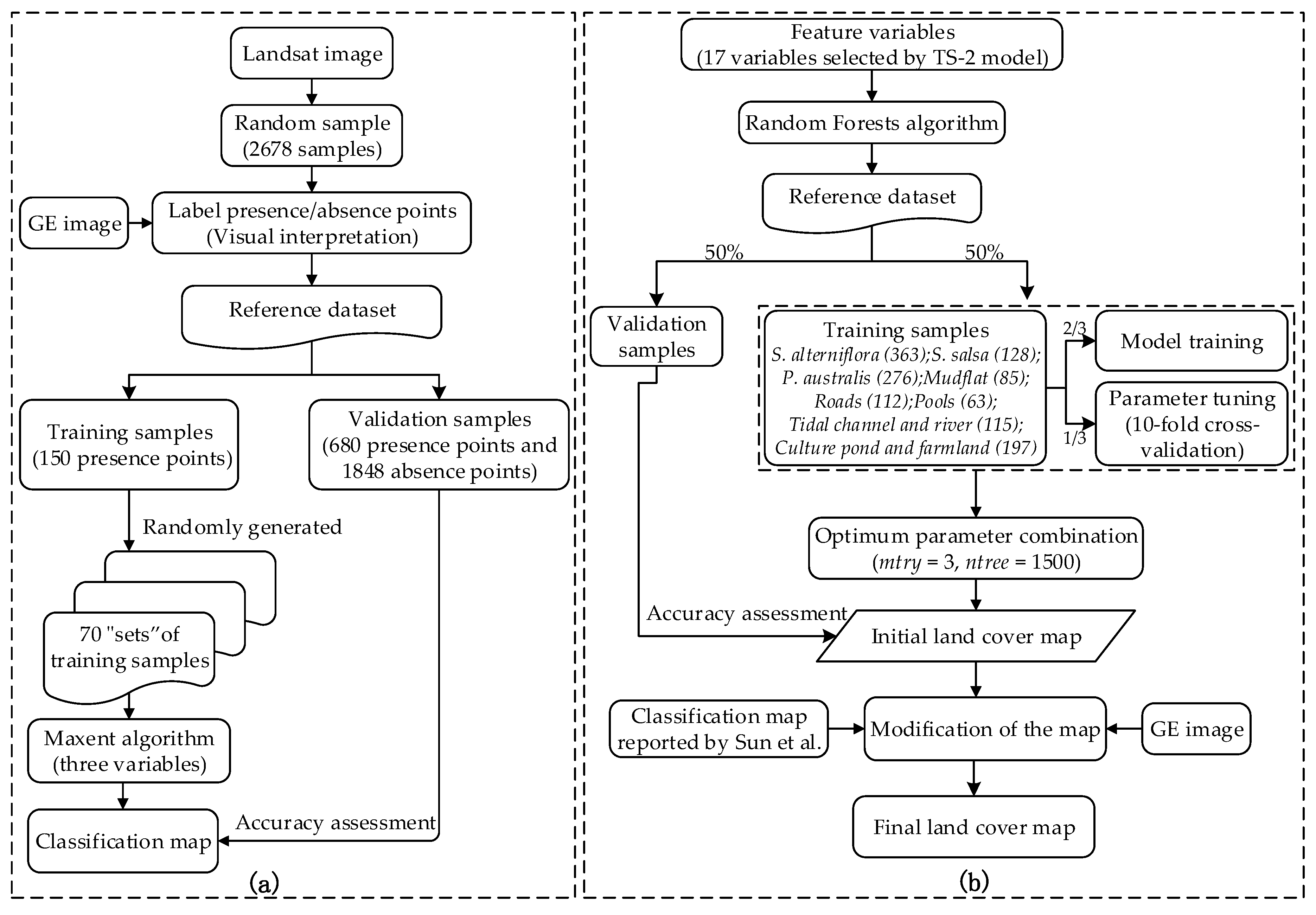
Figure 4.
The performance comparison of the Maxent-DPS model and the Maxent-AICc model with four evaluation indicators (Kappa, overall accuracy, specificity, sensitivity). The line chart on the left and the box plot on the right specific and overall performance of the Maxent-DPS model and the Maxent-AICc model under the 15 schemes (January–December, NDVI, TS-1, TS-2), respectively.
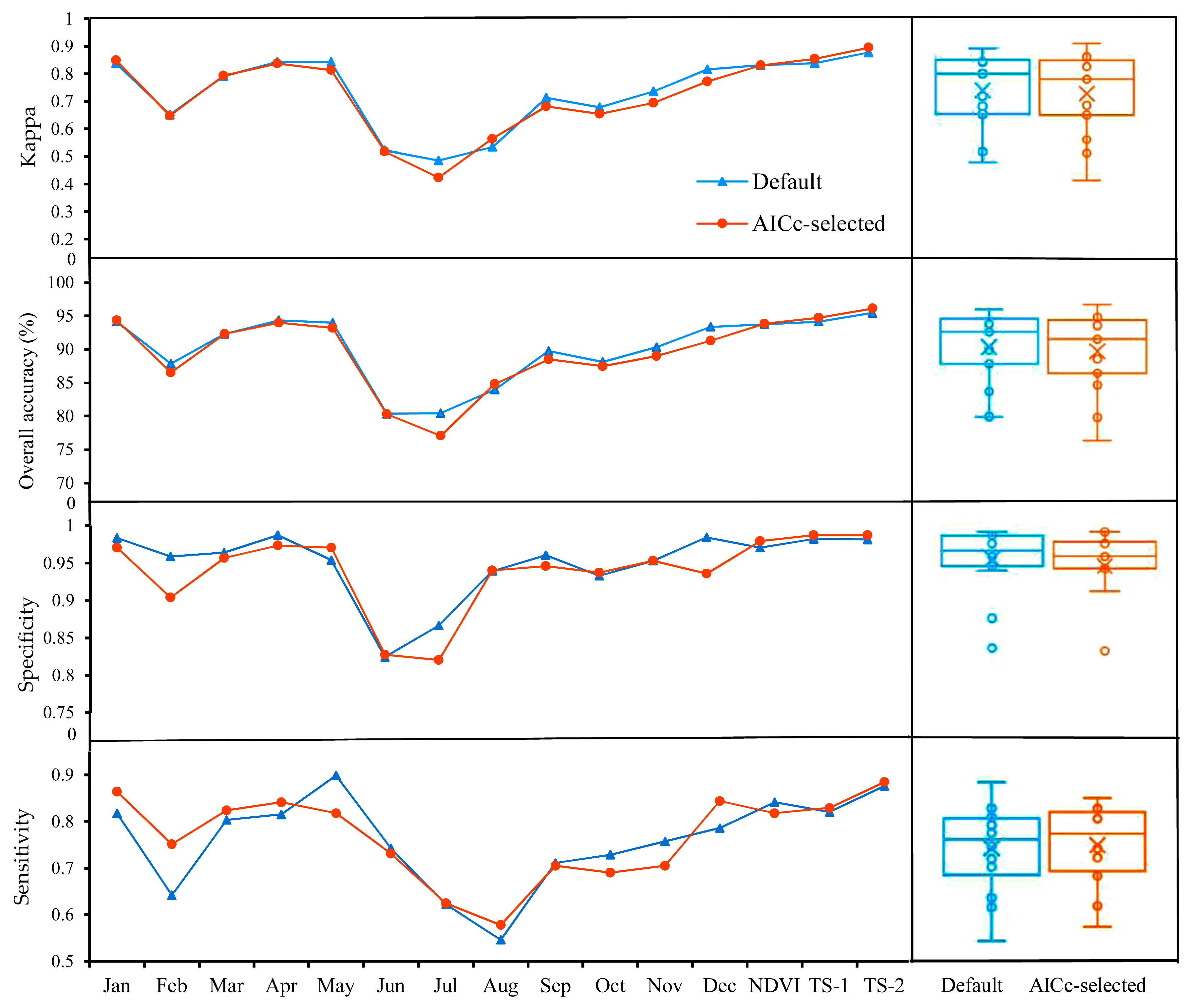
Figure 5.
Overall accuracy and Kappa coefficients for classification mapping of the 15 models in Experimental Setups 1–3.
Figure 5.
Overall accuracy and Kappa coefficients for classification mapping of the 15 models in Experimental Setups 1–3.
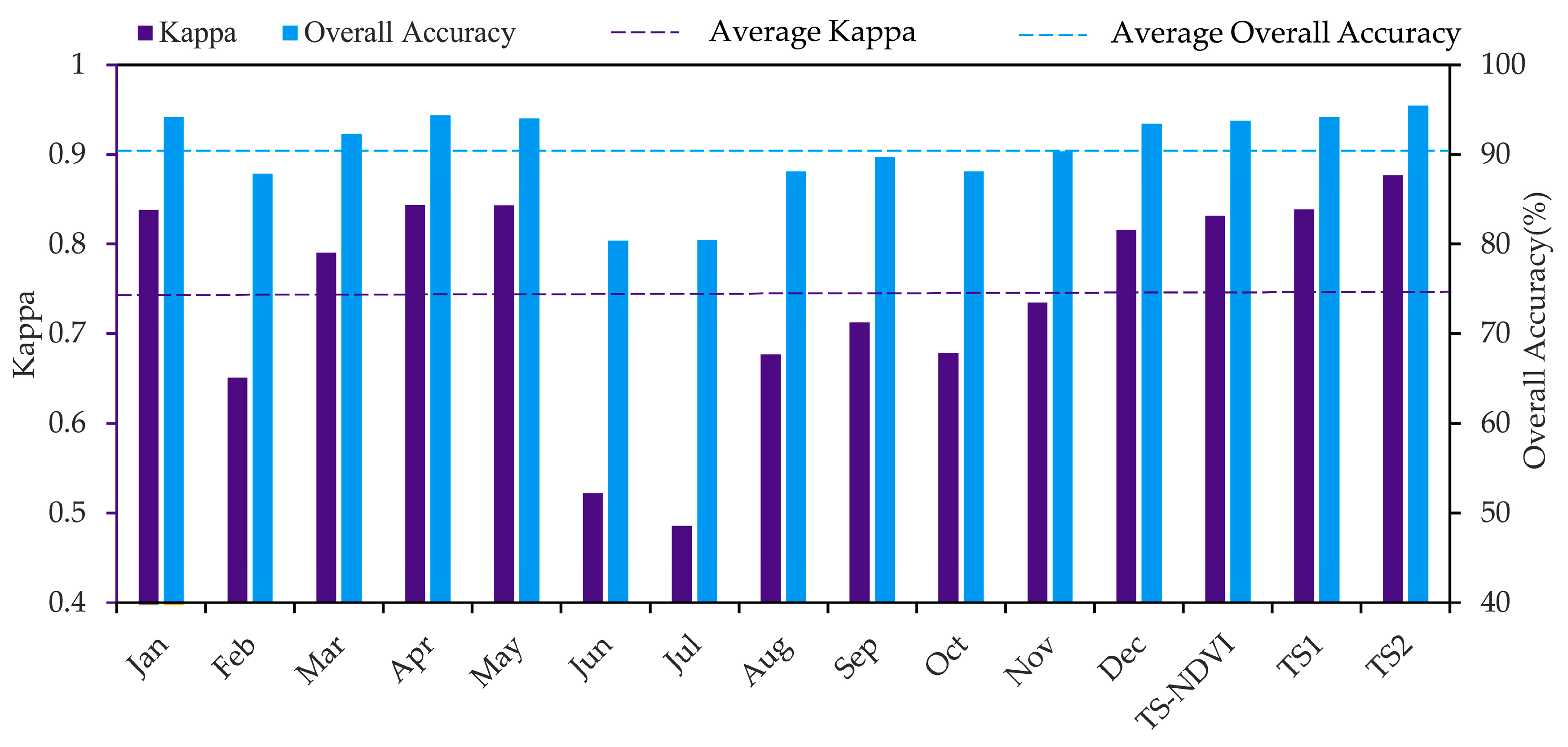
Figure 6.
Spectral reflectance curves of S. alterniflora and other land covers for each month in 2014. TCR: Tidal Channel and River. CPF: Culture Pond and Farmland.
Figure 6.
Spectral reflectance curves of S. alterniflora and other land covers for each month in 2014. TCR: Tidal Channel and River. CPF: Culture Pond and Farmland.
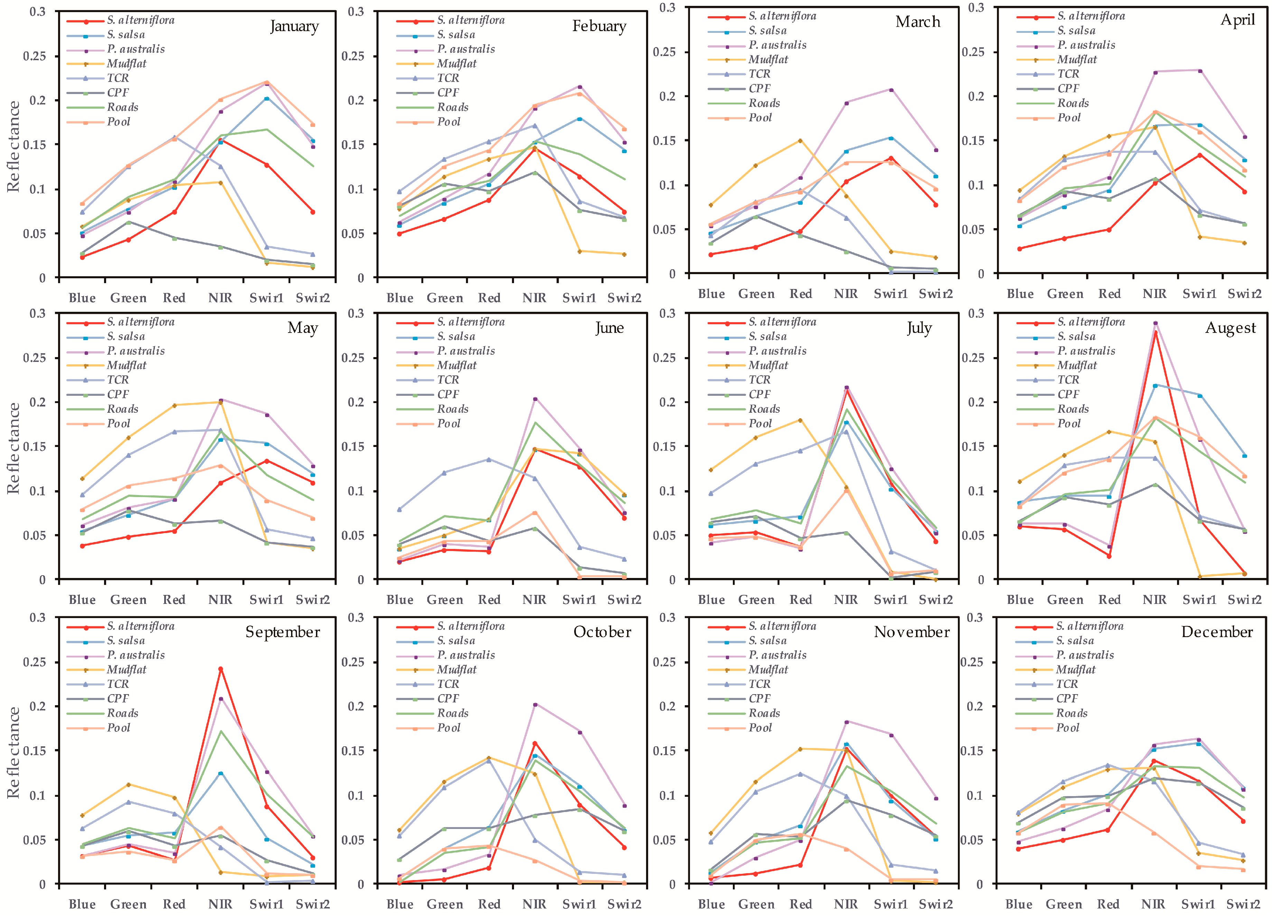
Figure 7.
Classification map of S. alterniflora based on Maxent under the 15 schemes (January–December, TS-NDVI, TS-1, TS-2) from Patterns 1–3. The land cover classification map is based on the GE image from 2014. The red circles show the misclassification errors.
Figure 7.
Classification map of S. alterniflora based on Maxent under the 15 schemes (January–December, TS-NDVI, TS-1, TS-2) from Patterns 1–3. The land cover classification map is based on the GE image from 2014. The red circles show the misclassification errors.

Figure 8.
Months’ importance sorted in descending order with the permutation importance value. The month importance was determined by summing the permutation importance value of all bands in each month (from AICc-selected models. (a) Months’ permutation importance from the first time-series model (TS-1); (b) months’ permutation importance from the second time-series model (TS-2); (c) months’ permutation importance from the third time-series model (TS-NDVI). The sum of the permutation importance value from the months with two time-series models below exceeds 90% of the total, depicted by the gray dotted line.
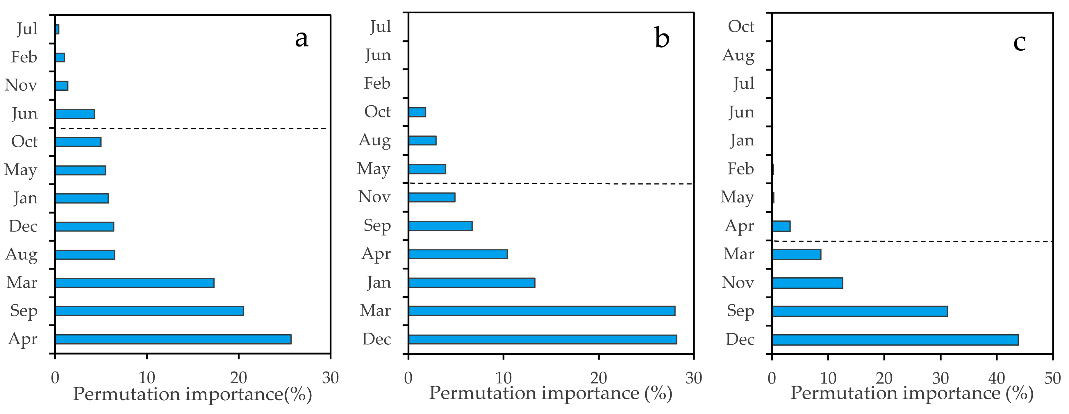
Figure 9.
Bands’ contributions are sorted in descending order with the permutation importance value output by the Time-Series 2 model. Bands (x-axis): the number stands for the month of the year, followed by the name of the variable. The sum of the permutation importance value from the months with two time-series models exceeds 90% of the total, depicted by the gray dotted line.

Figure 10.
Classification accuracies of the Maxent model using different numbers of band variables. The different models were created by removing the variable that had the least permutation importance value in TS-2 model from 17 to 1 in turn. The numbers of bands of the 17 variables were ordered by decreasing importance. For comparison, the figure also shows the classification accuracy of the best single-scene model (i.e., April).

Figure 11.
Performances of the time-series model using the number of training samples from 10 to 140. (a) Kappa, (b) Overall accuracy.
Figure 11.
Performances of the time-series model using the number of training samples from 10 to 140. (a) Kappa, (b) Overall accuracy.
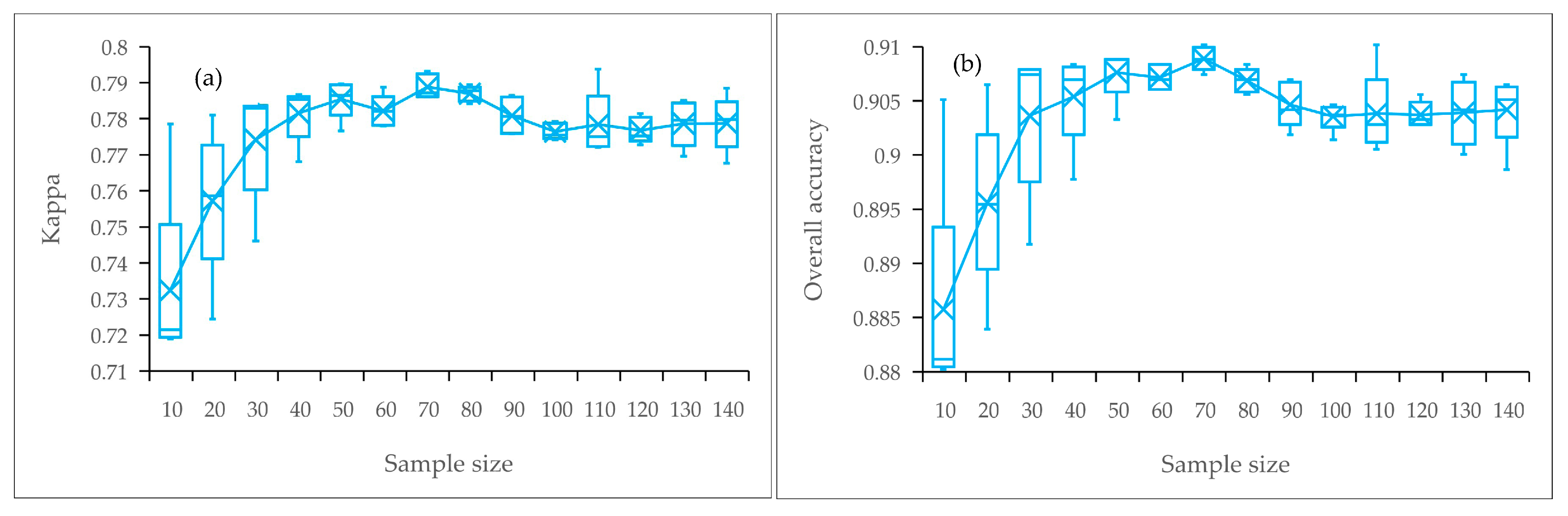
Figure 12.
Classification map for S. alterniflora on the middle coast of Jiangsu constructed using the compressed time-series model with the training samples of 10 and 70. (a1,b1,c1,d1,e1) are the identification results using 10 samples; (a2,b2,c2,d2,e2) are the identification results using 70 training samples; (a3,b3,c3,d3,e3) are the final land cover classification maps using the random forest classification method and visual interpretation; (f) overall view of the middle coast of Jiangsu; (g) overall view of the identification result using 70 training samples.
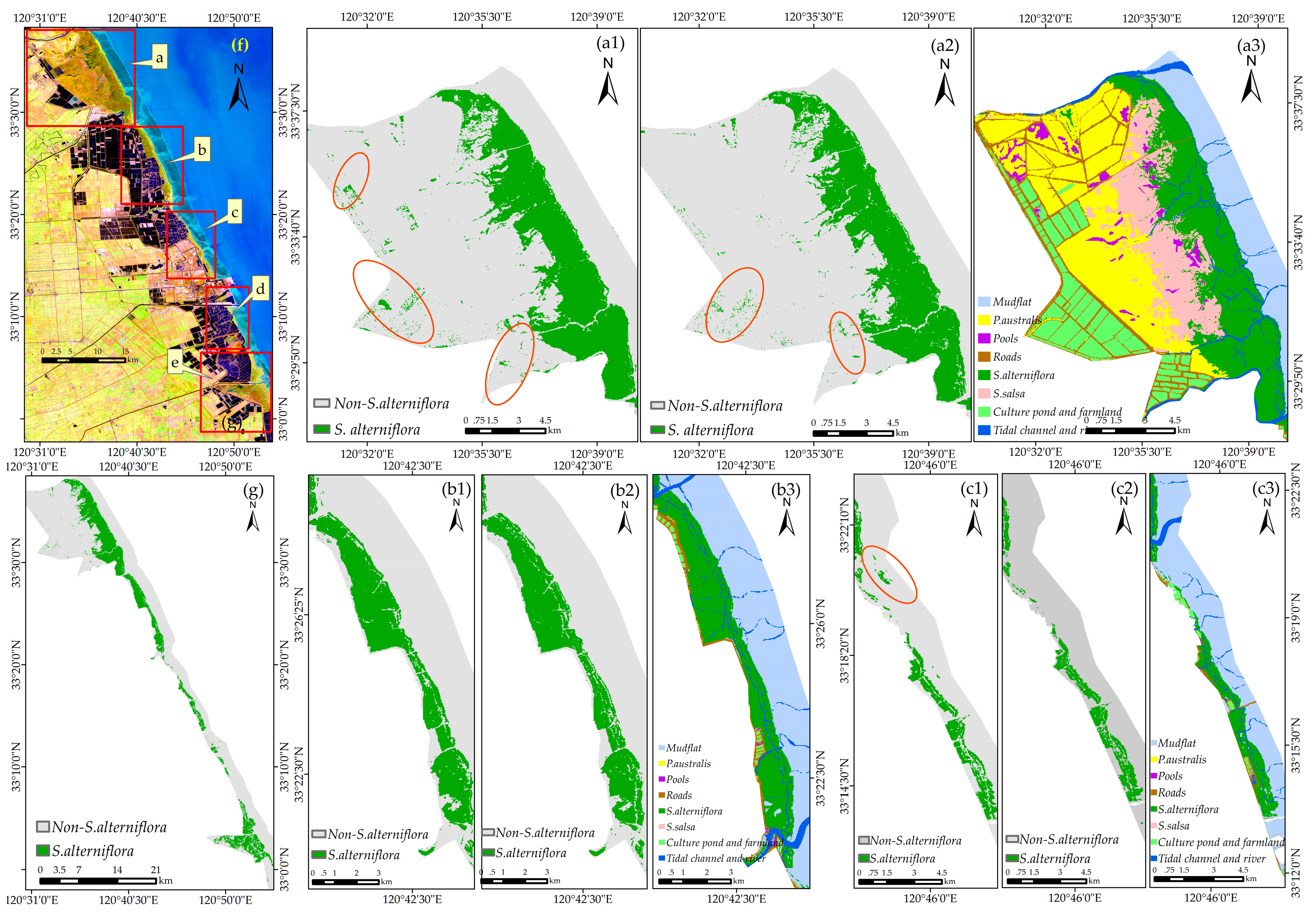

Table 1.
Information on the Landsat images used in this study.
| Description | Monthly Landsat Data | |||||||||||
|---|---|---|---|---|---|---|---|---|---|---|---|---|
| Sensor | OLI | ETM | OLI | ETM | OLI | ETM | ETM | ETM | OLI | OLI | ETM | OLI |
| Track number | 119/37 | 119/37 | 119/37 | 119/37 | 119/37 | 119/37 | 119/37 | 119/37 | 119/37 | 119/37 | 119/37 | 119/37 |
| Time | 01/27 | 02/20 | 3/16 | 04/25 | 05/03 | 06/12 | 07/14 | 08/12 | 09/08 | 10/26 | 11/03 | 12/13 |
Table 2.
Vegetation indices calculated from the Landsat data.
| Vegetable Indices | Formula |
|---|---|
| Normalized Difference Vegetation Index (NDVI) | NDVI = (NIR − Red)/(NIR + Red) |
| Difference Vegetation Index (DVI) | DVI = NIR − Red |
| Ratio Vegetation Index (RVI) | RVI = NIR/Red |
| Enhanced Vegetation Index (EVI) | EVI = 6.5 × (NIR − Red)/(NIR + 7.5 × Red − 2.5 × Blue + 1) |
Table 3.
Overall Accuracy (OA), kappa, sensitivity, specificity and the McNemar test results (|X| and p-value) for Maxent and BSVM methods. These accuracy indices of the proposed OCC methods under the 15 schemes of Setups 1–3 were calculated by the validation dataset.
Table 3.
Overall Accuracy (OA), kappa, sensitivity, specificity and the McNemar test results (|X| and p-value) for Maxent and BSVM methods. These accuracy indices of the proposed OCC methods under the 15 schemes of Setups 1–3 were calculated by the validation dataset.
| Models | Maxent | BSVM | McNemar Test to Compare Maxent and BSVM (p-Value) | ||||||
|---|---|---|---|---|---|---|---|---|---|
| OA (%) | Kappa | Sensitivity | Specificity | OA (%) | Kappa | Sensitivity | Specificity | ||
| January | 94.14 | 0.84 | 0.82 | 0.98 | 93.99 | 0.84 | 0.87 | 0.96 | 0.93 (p = 0.336) |
| February | 87.83 | 0.65 | 0.64 | 0.96 | 84.69 | 0.61 | 0.76 | 0.88 | 8.80 (p < 0.01) |
| March | 92.31 | 0.79 | 0.80 | 0.96 | 93.04 | 0.80 | 0.76 | 0.99 | 2.00 (p = 0.157) |
| April | 94.36 | 0.84 | 0.82 | 0.98 | 94.07 | 0.84 | 0.86 | 0.96 | 0.19 (p = 0.662) |
| May | 93.99 | 0.84 | 0.89 | 0.96 | 93.48 | 0.82 | 0.81 | 0.98 | 10.45 (p < 0.01) |
| June | 80.37 | 0.52 | 0.74 | 0.82 | 79.49 | 0.49 | 0.68 | 0.83 | 0.62 (p = 0.432) |
| July | 80.44 | 0.49 | 0.62 | 0.86 | 80.14 | 0.43 | 0.48 | 0.91 | 13.55 (p < 0.01) |
| August | 88.13 | 0.68 | 0.72 | 0.93 | 86.81 | 0.62 | 0.62 | 0.95 | 13.90(p < 0.01) |
| September | 89.74 | 0.71 | 0.71 | 0.96 | 90.77 | 0.74 | 0.74 | 0.97 | 6.53 (p < 0.01) |
| October | 88.13 | 0.68 | 0.73 | 0.93 | 89.16 | 0.69 | 0.71 | 0.95 | 17.69 (p < 0.01) |
| November | 90.32 | 0.74 | 0.75 | 0.95 | 90.11 | 0.72 | 0.69 | 0.97 | 22.74 (p < 0.01) |
| December | 93.41 | 0.82 | 0.79 | 0.98 | 93.33 | 0.82 | 0.86 | 0.96 | 17.28 (p < 0.01) |
| TS-1 | 94.14 | 0.84 | 0.82 | 0.98 | 94.29 | 0.84 | 0.79 | 0.99 | 1.51 (p = 0.218) |
| TS-2 | 95.46 | 0.88 | 0.87 | 0.98 | 95.89 | 0.89 | 0.87 | 0.97 | 0.94 (p = 0.330) |
| TS-NDVI | 93.77 | 0.83 | 0.84 | 0.97 | 92.97 | 0.80 | 0.75 | 0.99 | 1.79 (p = 0.072) |
Table 4.
Paired t-test for five pairs of accuracy indices (p = 0.05). Accuracy indices (Kappa, overall accuracy, sensitivity, specificity, omission) of the proposed OCC approaches of Maxent and BSVM under the 15 schemes of Setups 1–3.
Table 4.
Paired t-test for five pairs of accuracy indices (p = 0.05). Accuracy indices (Kappa, overall accuracy, sensitivity, specificity, omission) of the proposed OCC approaches of Maxent and BSVM under the 15 schemes of Setups 1–3.
| Accuracy indices | Mean | Paired Differences 95% Confidence Interval | t | df | Significance (Two-Tailed) | |
|---|---|---|---|---|---|---|
| Lower | Upper | |||||
| Kappa: BSVM—Maxent | −0.124 | −0.451 | 0.209 | −0.800 | 14 | 0.473 |
| OA: BSVM—Maxent | −0.164 | −0.036 | 0.003 | −1.731 | 14 | 0.105 |
| Specificity: BSVM—Maxent | −0.001 | −0.175 | 0.152 | −0.148 | 14 | 0.885 |
| Sensitivity: BSVM—Maxent | −0.496 | −0.967 | −0.002 | −2.258 | 14 | 0.400 |
| Omission: BSVM—Maxent | 0.851 | −0.007 | 0.872 | 1.824 | 14 | 0.900 |
Table 5.
Parameter settings of fifteen Maxent-AICc models generated by ENMeval. Note that for all Maxent-Default Parameter Set (DPS) in Maxent of Experimental Setups 1–3, the Feature Combinations (FC) were linear, quadratic and hinge, and the Regularization Multipliers (RM) was 1. L = Linear, Q = Quadratic, H = Hinge, P = Product and T = Threshold.
| Parameters | Experimental Setup 1 | Experimental Setup 2 | Experimental Setup 3 | ||||||||||||
|---|---|---|---|---|---|---|---|---|---|---|---|---|---|---|---|
| Jan | Feb | Mar | Apr | May | Jun | Jul | Aug | Sep | Oct | Nov | Dec | TS-1 | TS-2 | TS-NDVI | |
| FC | LQ | LQHP | LQH | LQH | LQHP | LQ | LQ | LQHP | LQH | LQ | L | L | LQH | LQH | LQ |
| RM | 1 | 1.5 | 3.5 | 2 | 2 | 2 | 2.5 | 2 | 4 | 1.5 | 2 | 2 | 4 | 1.5 | 2 |
Table 6.
Paired t-test for five pairs of accuracy indices (p = 0.05). Accuracy indices (kappa, overall accuracy, sensitivity, specificity, omission) of the Maxent-AICc model and Maxent-DPS model under the 15 schemes of Setups 1–3.
Table 6.
Paired t-test for five pairs of accuracy indices (p = 0.05). Accuracy indices (kappa, overall accuracy, sensitivity, specificity, omission) of the Maxent-AICc model and Maxent-DPS model under the 15 schemes of Setups 1–3.
| Accuracy indices | Mean | Paired Differences 95% Confidence Interval | t | df | Significance (Two-Tailed) | |
|---|---|---|---|---|---|---|
| Lower | Upper | |||||
| OA: Default—AICc | 0.011 | −0.003 | 0.025 | 1.671 | 14 | 0.117 |
| Kappa: Default—AICc | 0.005 | −0.001 | 0.012 | 1.992 | 14 | 0.066 |
| Specificity: Default—AICc | 0.010 | −0.002 | 0.225 | 1.774 | 14 | 0.098 |
| Sensitivity Default—AICc | −0.007 | −0.033 | 0.019 | −0.560 | 14 | 0.585 |
Table 7.
Bands’ importance of different months are ranked by the permutation importance value. The vegetation indexes are highlighted in green; the principal components are highlighted in yellow; and bands of the Tasseled Cap (TC) transform are highlighted in red.
Table 7.
Bands’ importance of different months are ranked by the permutation importance value. The vegetation indexes are highlighted in green; the principal components are highlighted in yellow; and bands of the Tasseled Cap (TC) transform are highlighted in red.
| Rank | Jan | Feb | Mar | Apr | May | Jun | Jul | Aug | Sep | Oct | Nov | Dec |
|---|---|---|---|---|---|---|---|---|---|---|---|---|
| 1 | TC2 | red | TC1 | NIR | PC2 | NIR | SWIR1 | TC3 | NDVI | red | NDVI | NDVI |
| 2 | SWIR1 | EVI | green | TC3 | NIR | TC2 | TC3 | PC2 | green | green | SWIR2 | green |
| 3 | PC2 | NIR | NDVI | green | blue | EVI | SWIR2 | PC1 | red | TC1 | SWIR1 | NIR |
© 2017 by the authors. Licensee MDPI, Basel, Switzerland. This article is an open access article distributed under the terms and conditions of the Creative Commons Attribution (CC BY) license (http://creativecommons.org/licenses/by/4.0/).
Share and Cite
MDPI and ACS Style
Liu, X.; Liu, H.; Gong, H.; Lin, Z.; Lv, S. Appling the One-Class Classification Method of Maxent to Detect an Invasive Plant Spartina alterniflora with Time-Series Analysis. Remote Sens. 2017, 9, 1120. https://doi.org/10.3390/rs9111120
AMA Style
Liu X, Liu H, Gong H, Lin Z, Lv S. Appling the One-Class Classification Method of Maxent to Detect an Invasive Plant Spartina alterniflora with Time-Series Analysis. Remote Sensing. 2017; 9(11):1120. https://doi.org/10.3390/rs9111120
Chicago/Turabian StyleLiu, Xiang, Huiyu Liu, Haibo Gong, Zhenshan Lin, and Shicheng Lv. 2017. "Appling the One-Class Classification Method of Maxent to Detect an Invasive Plant Spartina alterniflora with Time-Series Analysis" Remote Sensing 9, no. 11: 1120. https://doi.org/10.3390/rs9111120
Note that from the first issue of 2016, this journal uses article numbers instead of page numbers. See further details here.