On the Spatial and Temporal Sampling Errors of Remotely Sensed Precipitation Products

Jet Propulsion Laboratory, California Institute of Technology, 4800 Oak Grove Drive, MS 233-302E, Pasadena, CA 91109, USA
*
Author to whom correspondence should be addressed.
Remote Sens. 2017, 9(11), 1127; https://doi.org/10.3390/rs9111127
Submission received: 25 September 2017
/
Revised: 18 October 2017
/
Accepted: 2 November 2017
/
Published: 5 November 2017
(This article belongs to the Special Issue Remote Sensing Precipitation Measurement, Validation, and Applications)
Abstract
:Observation with coarse spatial and temporal sampling can cause large errors in quantification of the amount, intensity, and duration of precipitation events. In this study, the errors resulting from temporal and spatial sampling of precipitation events were quantified and examined using the latest version (V4) of the Global Precipitation Measurement (GPM) mission integrated multi-satellite retrievals for GPM (IMERG), which is available since spring of 2014. Relative mean square error was calculated at 0.1° × 0.1° every 0.5 h between the degraded (temporally and spatially) and original IMERG products. The temporal and spatial degradation was performed by producing three-hour (T3), six-hour (T6), 0.5° × 0.5° (S5), and 1.0° × 1.0° (S10) maps. The results show generally larger errors over land than ocean, especially over mountainous regions. The relative error of T6 is almost 20% larger than T3 over tropical land, but is smaller in higher latitudes. Over land relative error of T6 is larger than S5 across all latitudes, while T6 has larger relative error than S10 poleward of 20°S–20°N. Similarly, the relative error of T3 exceeds S5 poleward of 20°S–20°N, but does not exceed S10, except in very high latitudes. Similar results are also seen over ocean, but the error ratios are generally less sensitive to seasonal changes. The results also show that the spatial and temporal relative errors are not highly correlated. Overall, lower correlations between the spatial and temporal relative errors are observed over ocean than over land. Quantification of such spatiotemporal effects provides additional insights into evaluation studies, especially when different products are cross-compared at a range of spatiotemporal scales.
1. Introduction
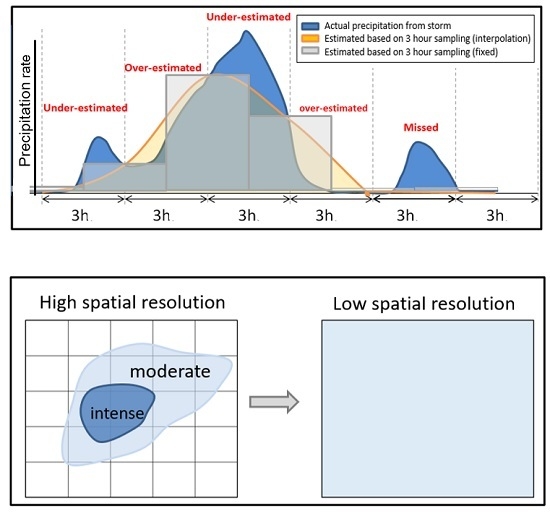
Accurate quantification of precipitation events is directly related to the temporal and spatial sampling of the observing system. A robust sensor with complete spatial coverage (e.g., radar or satellite) should be able to capture both temporal and spatial patterns of a precipitation system through its high spatiotemporal sampling. However, in practice, spatiotemporal sampling of observing systems is often limited and thus can result in errors in quantification of precipitation events. Figure 1 shows a schematic representation of temporal and spatial errors resulting from poor temporal (Figure 1a) and spatial (Figure 1b) sampling. In Figure 1a a hypothetical precipitation event (shown in blue curve) is sampled every three hours, which has been a common temporal sampling for satellite precipitation products (e.g., the Tropical Rainfall Measuring Mission (TRMM) 3B42 product [1]). Over- and under-estimation errors can be defined as the difference between the actual precipitation rate (blue curve) and precipitation rate from that can be approximated from the three-hour sampling (e.g., using linear interpolation or fixed values shown in yellow and gray color, respectively). Figure 1b shows an example of error resulting from poor spatial sampling (shown on the right) of a hypothetical precipitation event with regions of moderate and intense precipitation (shown on the left).
While both temporal and spatial sampling can result in errors, their magnitude can depend on the type of precipitation system. For example, precipitation from an isolated convective system may be more sensitive to the spatial and temporal sampling than precipitation from a stratiform system. The relative magnitude of temporal errors compared to spatial errors can also be different depending on precipitation environment and geographical conditions. For example, sampling errors associated with a fast-moving frontal system are expected to be larger than errors from a similar but slower-moving system. Furthermore, one can expect larger sampling errors over mountainous regions (e.g., due to sharp intensity gradient caused by orographic lifting) than a flat region.
The quantification of errors resulting from poor spatial and temporal sampling is important as they can largely affect several studies such as hydrologic simulations and applications. Nijssen and Lettenmaier [2] studied the effect of error in accumulated precipitation, due to periodic sampling of the precipitation rate, and found that streamflow errors were large for small drainage areas but decreased rapidly for drainage areas larger than about 50,000 km2. Steiner et al. [3] used ground radar data set over the Great Plains in the United States and evaluated the sampling-related uncertainty of rainfall estimate as a function of rainfall rate, domain size, accumulation period, and sampling period. Furthermore, in evaluation studies, precipitation products are often mapped onto a common spatiotemporal resolution prior to cross-comparison of products. What is often not carefully considered is that by smoothening of the higher resolution products, errors are added to the estimates that may lead to an unfair assessment of the high resolution products.
Here we quantify and examine the precipitation spatiotemporal sampling errors over global land and ocean and compare their relative magnitudes in different regions and seasons. This global analysis is not feasible using ground stations or radars, but has become possible through recent precipitation estimates from space that offer higher accuracy and spatiotemporal sampling than before.
2. Dataset and Method
2.1. Datasets
In this study, we used precipitation estimates from the latest version (V4) of the Global Precipitation Measurement (GPM) mission [4] integrated multi-satellite retrievals for GPM (IMERG) [5] product, released in spring of 2017. The GPM core observatory satellite was launched in February 2014 and carries two important instruments for precipitation measurements: (1) the dual-frequency precipitation radar (DPR) including Ku/Ka (13.6/35.5 GHz) bands and (2) the GPM microwave imager (GMI) which has 13 channels with frequencies ranging from 10 GHz to 183 GHz. These instruments have geographical coverage between 65° N–65° S. By blending precipitation estimates from multiple sensors (constellation of several radiometers and infrared imagers), IMERG provides gridded precipitation maps with high spatiotemporal resolution (0.1° × 0.1° every 0.5 h) within the latitude band 60° N–60° S since spring of 2014. However, the plan is to extend the product back in time to 1998, so it can cover the Tropical Rainfall Measuring Mission (TRMM) era. In brief, the retrieval method includes four main steps: (1) precipitation estimates from the GPM constellation radiometers are gridded, inter-calibrated to the GPM combined radar-radiometer product, and blended into half-hourly 0.1° × 0.1° fields; (2) maps of half-hourly IR precipitation rate are calculated using an IR-based precipitation retrieval method [6]; (3) by utilizing the Climate Prediction Center Morphing-Kalman Filter (CMORPH-KF) Lagrangian time interpolation scheme [7], MW and IR estimates are used to create half-hourly estimates, and (4) in the final run the multi-satellite half-hour estimates are adjusted so that they sum to a monthly satellite-gauge combination. The relatively high spatiotemporal resolution of IMERG and its global coverage provide a good opportunity to quantify quasi-global spatiotemporal sampling errors over land and ocean. Furthermore, by using IMERG, the present study provides insights on the amount of errors that can be added to the high resolution product (i.e., through smoothening it to a coarser resolution) prior to comparison with coarser resolution products.
2.2. Method
In order to determine the errors resulting from temporal and spatial sampling of precipitation events, precipitation maps at IMERG resolution were degraded to lower spatial (0.25° × 0.25°, 0.5° × 0.5°, and 1.0° × 1.0°) and temporal (three and six hours) resolutions. The spatial degradation was performed by averaging all fine resolution grids that fall inside the grid with coarser resolution. We also used a more sophisticated method by using the “griddata” function in MATLAB, which enables triangle-based linear interpolations. We found that the two methods yield fairly similar results and do not affect the conclusions of this study. Degradation of temporal resolution was performed by averaging all the times steps falling within the coarser time window. By assuming uniform distribution, the degraded precipitation maps were mapped onto IMERG original resolution (0.1° × 0.1° every 0.5 h) for comparison. These resolutions were selected as they are often produced by popular precipitation products. For example, TRMM 3B42 produces precipitation at 0.25° × 0.25° every three hours, reanalyses (e.g., MERRA; [8]) provide precipitation estimates at about 0.5° resolution, and the Global Precipitation Climatology Project (GPCP; [9]) product and several climate models offer precipitation at 1.0° × 1.0° resolution or coarser. The comparisons were conducted using two full years of data (2015–2016), separately for annual, extended boreal winter (November–March), and extended boreal summer (May–September) months. Root-mean-square error (RMSE) was used as a metric for errors between the degraded and original (i.e., 0.1° × 0.1° every 0.5 h) IMERG products. Since RMSE often increases with increases in precipitation rate, relative error defined by error (RMSE) divided by mean precipitation (from IMERG with its original resolution) was used. However, regions with mean daily precipitation of less than 0.5 mm/day were excluded from comparisons as at lower precipitation rates the relative errors become unstable. Note that one could also calculate BIAS, but BIAS is subject to the cancelation effect and thus a low seasonal or annual BIAS does not carry sufficient information about the magnitude of the overall errors.
3. Results
Figure 2a–c show maps of annual, winter, and summer mean precipitation rates for IMERG at a 0.1° × 0.1° resolution. Maps of percent relative-error for the different resolution-scenarios (described in Section 2.2) are shown in Figure 2d–o. The three-hour and six-hour scenarios are referred to in T3 and T6, respectively. The 0.5° × 0.5° is about five times coarser than IMERG original resolution in each dimension and hereafter is referred to as S5. Similarly, we refer to 1.0° × 1.0° as S10. To reduce redundancies we did not report the results of the 0.25° × 0.25° experiment. T3 shows that by degrading the temporal resolution of IMERG from 0.5 h to three hours, relative error exceed 30% in most regions. The errors are generally larger over land than ocean, especially over mountainous regions such as the Rocky Mountains in western North America, the Andes along the western edge of South America, and the Tibetan Plateau. By degrading the temporal resolution to six hours (T6), the errors will further increase, but the general pattern remains similar to T3. Large errors over ocean (e.g., over the Southern Ocean) are also observed, which is likely related to the fast moving precipitation systems affected by the polar and subtropical jet streams. The impact of spatial resolution degradation are displayed in the bottom two rows (Figure 2j–o): (a) land and mountainous region generally show higher relative errors than ocean, and (b) smaller relative error for both S5 and S10 are observed in high latitudes compared to the lower latitudes. This could be related to the fact that tropical regions contain a higher fraction of convective and small scale precipitation than higher latitudes [10]. Furthermore, there is a tendency towards less convective and more cellular cloud structures in high latitudes, resulting from cold air advection over warmer ocean surfaces [11], and thus precipitation in high latitudes might be less sensitive to changes in spatial resolution of the products. It should be noted that part of the observed zonal dependence of the results could be related to the use of equal latitude–longitude grids in IMERG, so a grid in lower latitudes covers a larger area than a grid in higher latitudes.
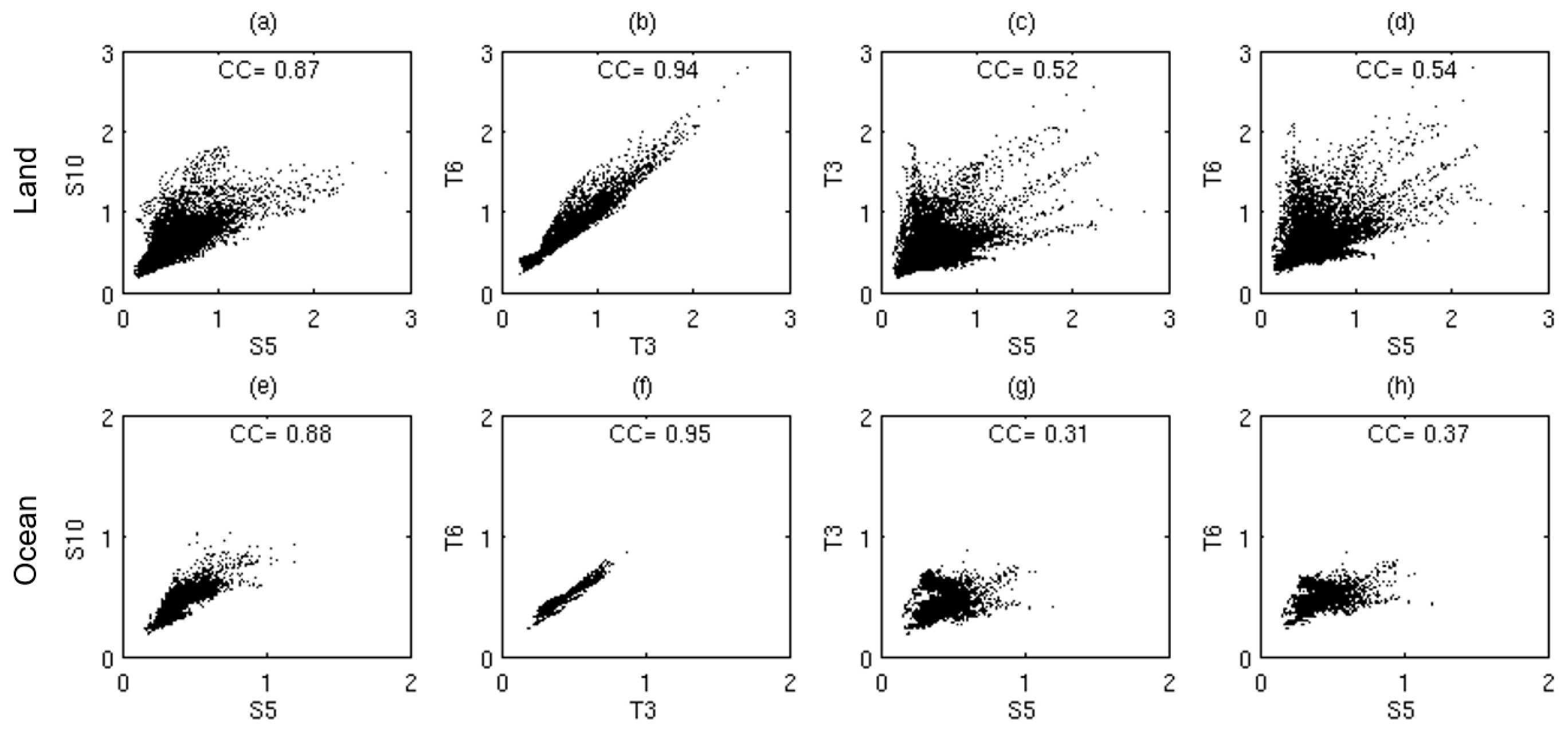
Figure 2 suggests that spatial and temporal relative errors can have different patterns. This can be better seen in the scatter plots of different pairs of relative errors (e.g., S5, S10, T3, and T6) shown in Figure 3. The Pearson correlation coefficients (CC) between the pairs are also shown in each panel to quantify the relationships. Overall, higher correlations between the spatial and temporal relative errors are observed over land than over ocean. This might be partly related to the fact that, over some regions (e.g., topographically complex areas), both spatial and temporal degradation cause large errors (see Figure 3).
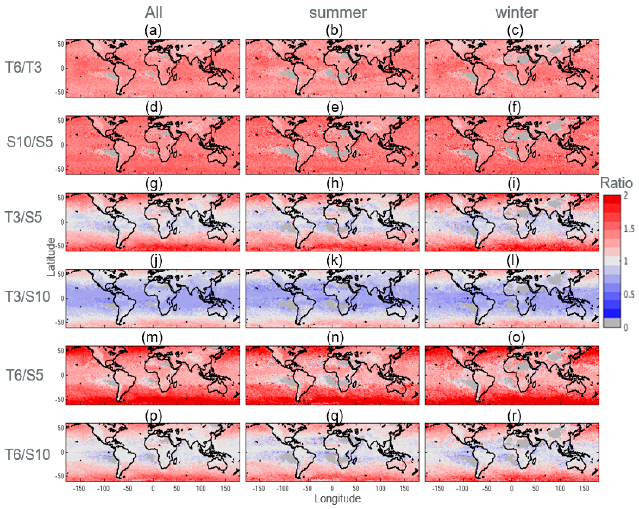
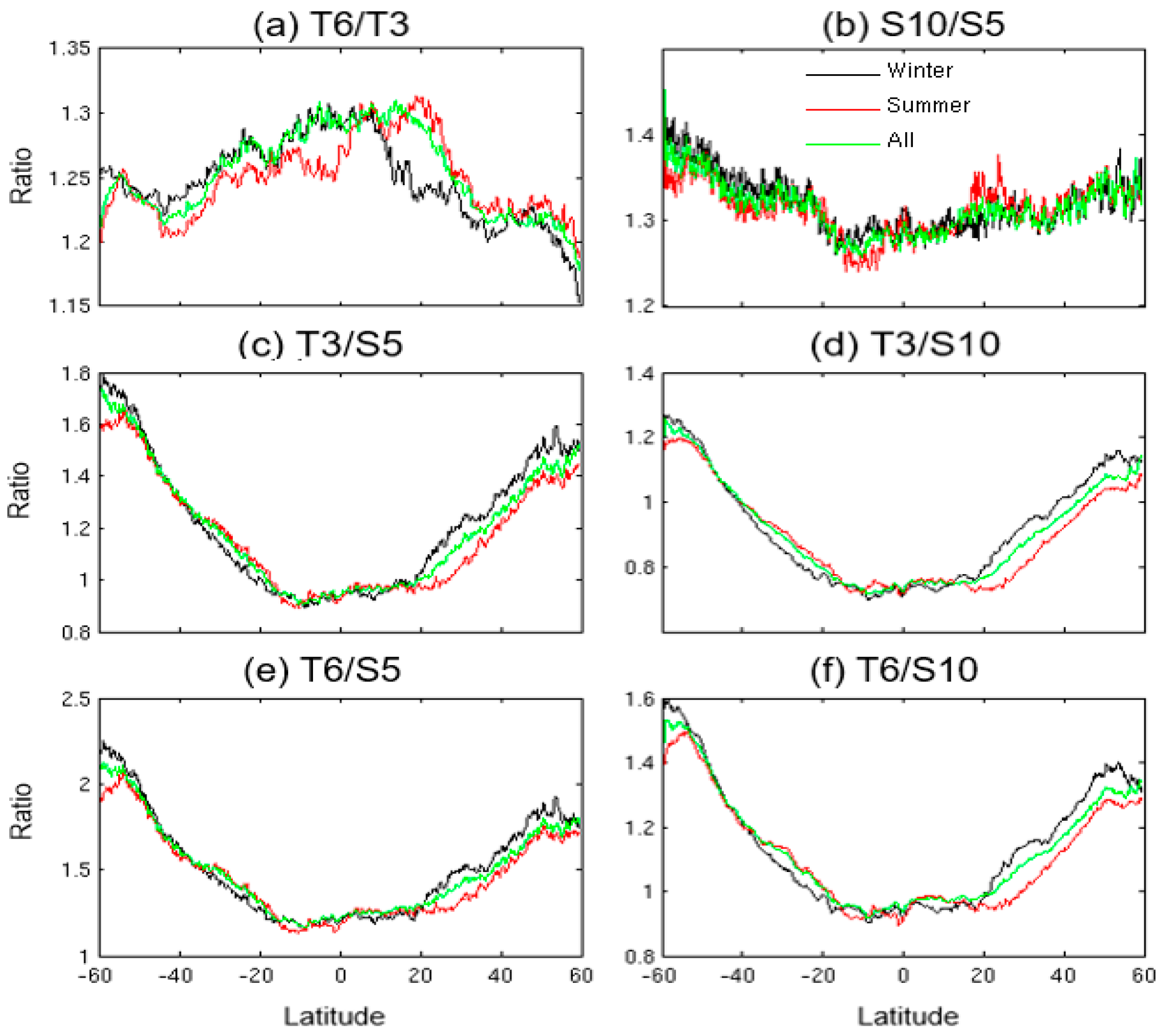
We recognized that, even after removing areas with low mean precipitation rate, some regions display large relative errors mainly due to dividing the errors by small mean precipitation rates (e.g., regions around tropical subsidence zone). In order to mitigate this effect we also plotted ratios of relative errors that are shown in Figure 4. As expected T6 shows higher relative error than T3, and S10 shows higher relative error than S5. In fact, these ratios (T6/T3 and S10/S5) are fairly uniform across land and ocean and for different seasons. The ratios between temporal and spatial relative errors are especially interesting as T3/S5 suggests that relative error of T3 is larger than S5 over high latitudes, but is equal or less in lower latitudes. Even T3/S10 shows that the relative error of T3 exceeds S10 over ocean between latitudes 50° and 60° in both hemispheres. It was found that T6/S5 is always greater than one over land and ocean and across all seasons, while in large regions over tropical ocean, and over land T6 and S10 show similar error ratios.
Figure 4 provides insights on how relative errors due to degradation of temporal and spatial resolution are compared globally. While seasonal differences exist, they are not easily observed in Figure 4. The differences can be better seen in zonal mean plots of the relative-error ratios shown separately over land (Figure 5) and ocean (Figure 6).
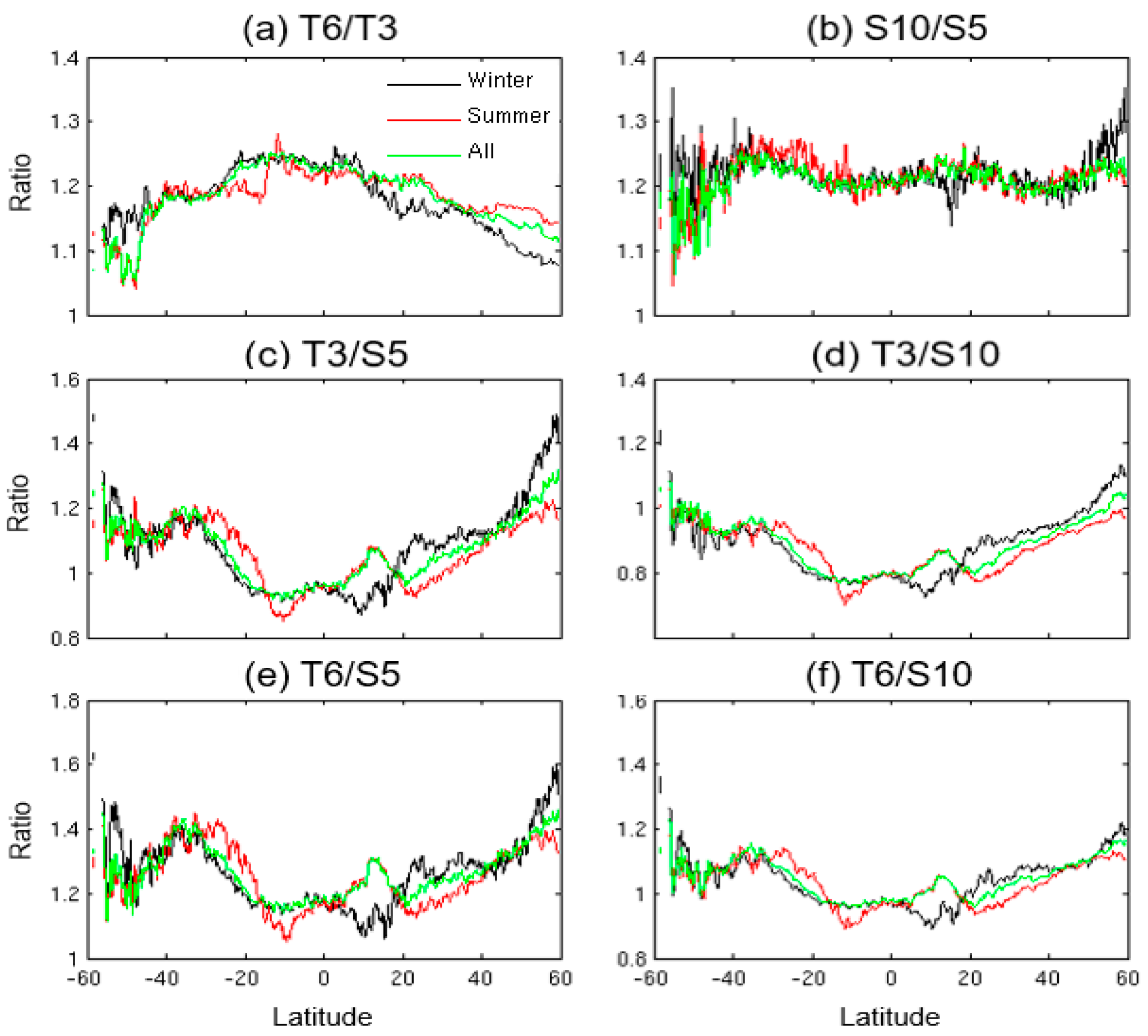
Figure 5a shows that relative error of T6 is almost 20% larger than T3 over tropical land and gradually decreases to about 10% in higher latitudes. This ratio is also larger in warm seasons than cold seasons. Figure 6a shows a similar pattern over ocean, but ratios are about 10% larger than over land (e.g., ~30% instead of 20% and 20% instead of 10%). Over land, relative error of S10 is about 20–25% larger than S5 within 40°S–40°N (Figure 5b). Poleward of 40°N this ratio increases in winter (30%), but remains almost the same in summer. The results over land area south of 40° S is unstable due to limited land areas. Over ocean relative error of S10 is about 25% larger than S5 in the tropics and gradually increases by moving towards higher latitudes (e.g., ~40% near 60° S). Figure 5 shows that over land relative error of T6 is larger than S5 across all latitudes, while T6 has larger relative error than S10 only poleward of ~20°S/N. Similarly, the relative error of T3 exceeds S5 poleward of ~20°S/N, but does not exceed S10, except at very high latitudes. Similar results are also seen over ocean, but the ratios are generally larger and less sensitive to seasonal changes (See Figure 6c,d).
Figure 5 and Figure 6 also show that the seasonal sensitivity of the results is generally larger over tropical land than tropical ocean, which can be inferred from the wider spread of the winter, summer, and all-season plots. In higher latitudes, the effect of seasonal differences is large over both land and ocean. This suggests that, in order to accurately account for spatiotemporal errors, it is important to perform the analyses by region and season, separately over land and ocean.
4. Summary and Concluding Remarks
In this study, the errors resulted from temporal and spatial sampling of precipitation events were investigated using the latest version (V4) of IMERG, providing precipitation estimates at 0.1° × 0.1° resolution every 30 min within the latitude band 60°N–60°S since spring of 2014. RMSE divided by mean precipitation was used to calculate climatology errors at 0.1° × 0.1° every 0.5 h between the degraded (temporally and spatially) and original IMERG products. The temporal and spatial degradation was performed by producing three hour (T3), six-hour (T6), 0.5° × 0.5° (S5), and 1.0° × 1.0° (S10) maps from IMERG. To enhance the stability of results, regions with annual or seasonal mean precipitation less than 0.5 mm/day were excluded from comparisons. The study was conducted using two years (2015–2016) of data, separately for all seasons, winter, and summer months. The results generally show larger errors over land than ocean, especially over mountainous regions. The relative error of T6 is almost 20% larger than T3 over tropical land and gradually decreases to about 10% in higher latitudes. Over land relative error of T6 is larger than S5 across all latitudes, while T6 has larger relative error than S10 only poleward of ~20°S/N. Similarly, the relative error of T3 exceeds S5 poleward of ~20°S/N, but does not exceed S10, except at very high latitude. Similar results are also seen over ocean, but the ratios are generally larger and less sensitive to seasonal changes (see Figure 6c,d). Furthermore, we found that the spatial and temporal relative errors are not necessarily correlated. Overall, lower correlations between the spatial and temporal relative errors are observed over ocean than over land.
We would like to emphasize that in addition to product-specific algorithmic errors, in practice [2,12] one should consider errors that can be originated from differences in spatiotemporal resolutions of products. For example, in mountainous basins, products that offer coarse spatiotemporal resolution may result in large errors in hydrologic simulations, despite the accuracy of the retrieval method used in these products. Even a spatial resolution of 0.1° × 0.1° may not be sufficient in such regions. Nevertheless, it is important to recognize that creating gridded products with finer spatial resolution than what input level-two products offer may not be suitable. While in this study we limited our analysis to few popular spatial and temporal resolutions, further analysis can include other resolutions and can be performed over a specific region [13], watershed, or at an event scale. Such analyses can provide additional insights on the type of observing systems or products needed for various studies.
Acknowledgments
The research described in this paper was carried out at the Jet Propulsion Laboratory, California Institute of Technology, under a contract with the National Aeronautics and Space Administration.
Author Contributions
Ali Behrangi conceived and designed the experiments; Ali Behrangi and Yixin Wen analyzed the data and performed the experiment; Ali Behrangi and Yixin Wen wrote the paper.
Conflicts of Interest
The authors declare no conflict of interest.
Abbreviations
The following abbreviations are used in this manuscript:
| CC | correlation coefficients |
| GPCP | Global Precipitation Climatology Project |
| GPM | Global Precipitation Measurement |
| IMERG | integrated multisatellite retrievals for GPM |
| RMSE | root-mean-square error |
| S10 | spatial degradation by 1.0° × 1.0° |
| S5 | spatial degradation by 0.5° × 0.5° |
| T3 | temporal degradation by three hours |
| T6 | temporal degradation by six hours |
| TRMM | Tropical Rainfall Measuring Mission |
References
- Huffman, G.J.; Adler, R.F.; Bolvin, D.T.; Gu, G.J.; Nelkin, E.J.; Bowman, K.P.; Hong, Y.; Stocker, E.F.; Wolff, D.B. The TRMM multisatellite precipitation analysis (TMPA): Quasi-global, multiyear, combined-sensor precipitation estimates at fine scales. J. Hydrometeorol. 2007, 8, 38–55. [Google Scholar] [CrossRef]
- Nijssen, B.; Lettenmaier, D.P. Effect of precipitation sampling error on simulated hydrological fluxes and states: Anticipating the global precipitation measurement satellites. J. Geophys. Res. Atmos. 2004, 109, 265–274. [Google Scholar] [CrossRef]
- Steiner, M.; Bell, T.L.; Zhang, Y.; Wood, E.F. Comparison of two methods for estimating the sampling-related uncertainty of satellite rainfall averages based on a large radar dataset. J. Clim. 2003, 16, 3759–3778. [Google Scholar] [CrossRef]
- Skofronick-Jackson, G.; Petersen, W.A.; Berg, W.; Kidd, C.; Stocker, E.F.; Kirschbaum, D.B.; Kakar, R.; Braun, S.A.; Huffman, G.J.; Iguchi, T.; et al. The global precipitation measurement (GPM) mission for science and society. Bull. Am. Meteorol. Soc. 2016. [Google Scholar] [CrossRef]
- Huffman, G.J.; Bolvin, D.; Braithwaite, D.; Hsu, K.; Joyce, R.; Kidd, C.; Nelkin, E.; Xie, P.P. Integrated Multi-Satellite Retrievals for GPM (IMERG): Algorithm Theoretical Basis Document (ATBD) Version 4.5. 2015. Available online: http://pmm.nasa.gov/sites/default/files/document_files/IMERG_ATBD_V4.5.pdf (accessed on 18 October 2017).
- Hong, Y.; Hsu, K.L.; Sorooshian, S.; Gao, X.G. Precipitation estimation from remotely sensed imagery using an artificial neural network cloud classification system. J. Appl. Meteorol. 2004, 43, 1834–1852. [Google Scholar] [CrossRef]
- Joyce, R.J.; Xie, P. Kalman filter based cmorph. J. Hydrometeorol. 2011, 12, 1547–1563. [Google Scholar] [CrossRef]
- Bosilovich, M.G.; Robertson, F.R.; Chen, J. Global energy and water budgets in MERRA. J. Clim. 2011, 24, 5721–5739. [Google Scholar] [CrossRef]
- Huffman, G.J.; Adler, R.F.; Morrissey, M.M.; Bolvin, D.T.; Curtis, S.; Joyce, R.; McGavock, B.; Susskind, J. Global precipitation at one-degree daily resolution from multisatellite observations. J. Hydrometeorol. 2001, 2, 36–50. [Google Scholar] [CrossRef]
- Houze, R.A. Stratiform precipitation in regions of convection: A meteorological paradox? Bull. Am. Meteorol. Soc. 1997, 78, 2179–2196. [Google Scholar] [CrossRef]
- Klepp, C.; Bumke, K.; Bakan, S.; Bauer, P. Ground validation of oceanic snowfall detection in satellite climatologies during lofzy. Tellus A 2010, 62, 469–480. [Google Scholar] [CrossRef] [Green Version]
- Behrangi, A.; Khakbaz, B.; Jaw, T.C.; AghaKouchak, A.; Hsu, K.; Sorooshian, S. Hydrologic evaluation of satellite precipitation products over a mid-size basin. J. Hydrol. 2011, 397, 225–237. [Google Scholar] [CrossRef]
- Asong, Z.E.; Razavi, S.; Wheater, H.S.; Wong, J.S. Evaluation of integrated multisatellite retrievals for GPM (IMERG) over southern Canada against ground precipitation observations: A preliminary assessment. J. Hydrometeorol. 2017, 18, 1033–1050. [Google Scholar] [CrossRef]
Figure 1.
A schematic representation of temporal and spatial errors resulted from poor temporal (a) and spatial (b) sampling. The low resolution grid in Figure 1b (right side) is shown in light blue that represents average of intense (shown in dark blue), moderate, and zero (in white) rain rate shown in the left panel.
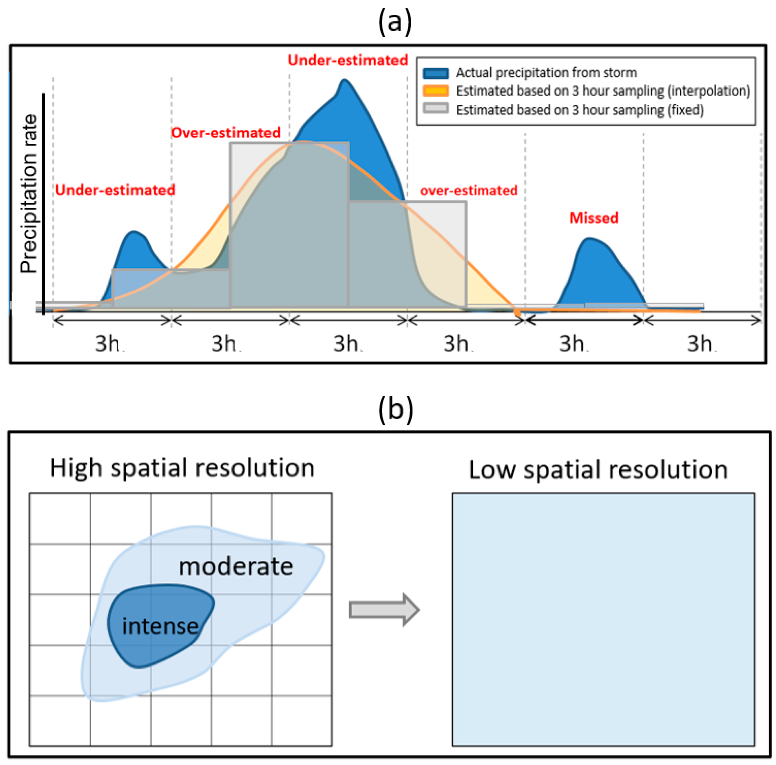
Figure 2.
(a–c) Maps of annual, winter, and summer mean precipitation rates and (d–o) the corresponding percent relative-error for the different resolution scenarios.
Figure 2.
(a–c) Maps of annual, winter, and summer mean precipitation rates and (d–o) the corresponding percent relative-error for the different resolution scenarios.
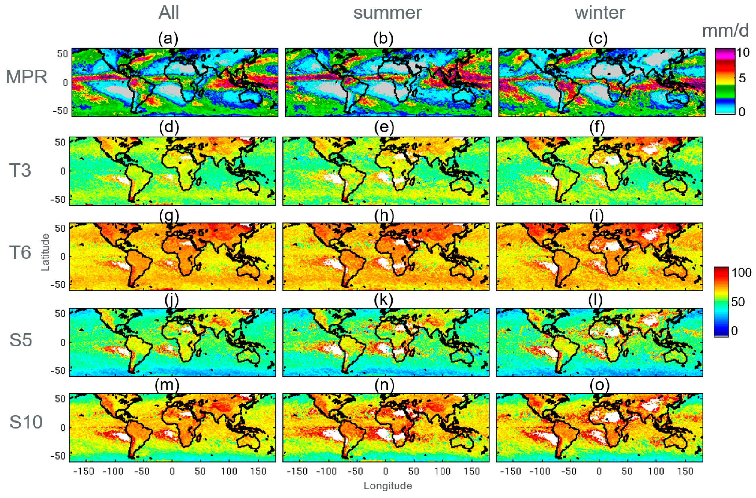
Figure 3.
Scatter plots constructed from different spatial and temporal relative errors. Correlation coefficients (CC) are shown in each panel. Note the axes show relative errors and are dimensionless. The top and bottom rows represent land and ocean, respectively.
Figure 3.
Scatter plots constructed from different spatial and temporal relative errors. Correlation coefficients (CC) are shown in each panel. Note the axes show relative errors and are dimensionless. The top and bottom rows represent land and ocean, respectively.

Figure 4.
Ratio of relative errors calculated for different combination of T3, T6, S5, and S10.

Figure 5.
Zonal mean plots of the relative-error ratios shown separately over land.

Figure 6.
Similar to Figure 4, but over ocean.
Figure 6.
Similar to Figure 4, but over ocean.

© 2017 by the authors. Licensee MDPI, Basel, Switzerland. This article is an open access article distributed under the terms and conditions of the Creative Commons Attribution (CC BY) license (http://creativecommons.org/licenses/by/4.0/).
Share and Cite
MDPI and ACS Style
Behrangi, A.; Wen, Y. On the Spatial and Temporal Sampling Errors of Remotely Sensed Precipitation Products. Remote Sens. 2017, 9, 1127. https://doi.org/10.3390/rs9111127
AMA Style
Behrangi A, Wen Y. On the Spatial and Temporal Sampling Errors of Remotely Sensed Precipitation Products. Remote Sensing. 2017; 9(11):1127. https://doi.org/10.3390/rs9111127
Chicago/Turabian StyleBehrangi, Ali, and Yixin Wen. 2017. "On the Spatial and Temporal Sampling Errors of Remotely Sensed Precipitation Products" Remote Sensing 9, no. 11: 1127. https://doi.org/10.3390/rs9111127
Note that from the first issue of 2016, this journal uses article numbers instead of page numbers. See further details here.