A Flexible Algorithm for Detecting Challenging Moving Objects in Real-Time within IR Video Sequences

1
Department of Information Engineering, University of Pisa, Via G. Caruso 16, 56122 Pisa, Italy
2
Italian Naval Academy, Viale Italia 72, 57127 Livorno, Italy
*
Author to whom correspondence should be addressed.
Remote Sens. 2017, 9(11), 1128; https://doi.org/10.3390/rs9111128
Submission received: 9 September 2017
/
Revised: 23 October 2017
/
Accepted: 1 November 2017
/
Published: 6 November 2017
(This article belongs to the Special Issue Instrumenting Smart City Applications with Big Sensing and Earth Observatory Data: Tools, Methods and Techniques)
Abstract
:Real-time detecting moving objects in infrared video sequences may be particularly challenging because of the characteristics of the objects, such as their size, contrast, velocity and trajectory. Many proposed algorithms achieve good performances but only in the presence of some specific kinds of objects, or by neglecting the computational time, becoming unsuitable for real-time applications. To obtain more flexibility in different situations, we developed an algorithm capable of successfully dealing with small and large objects, slow and fast objects, even if subjected to unusual movements, and poorly-contrasted objects. The algorithm is also capable to handle the contemporary presence of multiple objects within the scene and to work in real-time even using cheap hardware. The implemented strategy is based on a fast but accurate background estimation and rejection, performed pixel by pixel and updated frame by frame, which is robust to possible background intensity changes and to noise. A control routine prevents the estimation from being biased by the transit of moving objects, while two noise-adaptive thresholding stages, respectively, drive the estimation control and allow extracting moving objects after the background removal, leading to the desired detection map. For each step, attention has been paid to develop computationally light solution to achieve the real-time requirement. The algorithm has been tested on a database of infrared video sequences, obtaining promising results against different kinds of challenging moving objects and outperforming other commonly adopted solutions. Its effectiveness in terms of detection performance, flexibility and computational time make the algorithm particularly suitable for real-time applications such as intrusion monitoring, activity control and detection of approaching objects, which are fundamental task in the emerging research area of Smart City.
1. Introduction
Automatic detection of moving objects is a key task in numerous fields, such as video surveillance, and computer vision. Using steady infrared (IR) cameras is one of the most effective and cheapest ways to achieve it.
In many applications, detection may be particularly challenging, mainly due to the characteristics of the moving objects. On the one hand, their size can be very small or can appear small because of the distance from the camera, thus the information they provide is limited to the value of a few pixels [1]. On the other hand, the size can be rather large, generating problems for those algorithms that exploit the variation of pixels intensity over time: if a portion of a large and not textured object overlaps in two different frames, this is likely not to be detected (self-deletion problem) [2]. Moreover, the contrast of the moving objects with respect to the background can be low (dim objects) and, therefore, these can be confused with it [3]. Even the movement of the objects can make the detection difficult, especially for those algorithms based on tracking information [4]. For example, a slowly moving object can be mistaken for a part of the background, whereas quick changes in its trajectory are likely to affect the estimate of the future position from past detections. Furthermore, the characteristics of the objects and their movements are often unknown, thus no additional information can be exploited to circumscribe the problem. Another challenge is represented by time constraints. In numerous contexts, real-time detection is required and low-performing processors are available. Thus, computationally heavy solutions are not suitable even if efficient in terms of detection capability.
A flexible algorithm, capable to handle all these problems at the same time, would be very useful in circumstances where great versatility is required. Unfortunately, even though many algorithms for detecting moving objects from a steady camera have been proposed in the literature, either for optical or for IR video sequences, these generally account only for some of the above-mentioned problems, neglecting the others. Such algorithms can be classified in two broad categories, the ones based on track-before-detect (TBD) strategies and the ones based on detect-before-track (DBT) strategies. TBD strategies aim to track the candidate moving objects before declaring them detected. Typical TBD approaches are spatial-temporal matched filters [5], particle filters [6], dynamic programming [7], histogram probabilistic multi-hypothesis tracking [8], probabilistic data association [9] and multidimensional Hough transform [10]. They generally reach better detection rates than DBT ones, since they integrate data over space and time jointly, achieving a higher signal-to-noise ratio (SNR). Nonetheless, some of these approaches succeed only if the moving objects satisfy specific conditions. For example, some approaches [6,10] fail if the objects deviate from an initially assumed range of velocity or from some hypothesized types of trajectory, whereas other approaches [8] suffer from a deterioration of the performance in the presence of fast objects [11]. Moreover, TDB algorithms require high computational time, thus they are generally not suitable for real-time applications using low cost hardware [12].
DBT strategies are usually faster than TBD ones, since they do not attempt to integrate the signal in the space-time domain. A further classification of the DBT strategies can be made by dividing those that exploit the spatial domain from those that exploit the temporal domain. The ones based on spatial analysis aim to detect salient features within every frame. Some of these techniques can also be borrowed from works in the hyperspectral imagery [13], or even from sonar imagery [14,15]. However, they are not optimal for the case in question, since they do not exploit the motion of the objects to be detected [15,16,17], or exploit it only for validating and strengthening previous decisions [18,19]. Moreover, they require a significant contrast between the objects and their surrounding background, thus they are not effective in the presence of dim objects.
Instead, strategies based on temporal analysis aim to evaluate if any significant change occurs in the scene over time. They are particularly suitable to detect moving objects, since they inherently exploit the motion of the objects. In addition, they do not strictly require a high object-background contrast, because they are able to enhance it by integrating more frames together. However, many of these strategies work correctly only under some prior assumptions and they can deal only with some of the possible challenges that can be encountered in practical applications. In [20], the traditional method of frame differencing is presented, together with some variants that aim to increase its robustness to noise. These techniques are very simple and fast, but need to be adjusted with respect to the size, the velocity and, in some cases, also the intensity of the objects. Thus, objects with different characteristics from the expected ones are likely to not be detected. In [21], the bivariate cubic facet fitting is used as a second stage, for refining the results of a first frame differencing stage. Instead, in [22], frame differencing is used for removing false alarms, after an initial rough detection based on Canny algorithm and morphological filtering. Both strategies have proven to achieve a considerable increase of the detection rate with respect to the techniques solely based on frame differencing. However, in [21], only small objects, hotter than the background, can be correctly detected, while, in [22], the Canny method assumes that the object-background contrast is high, making dim objects difficult to be detected.
Other strategies differ from frame differencing, aiming at a robust estimation of the background, based on multiple observations of the scene. The background is then subtracted from the original frames to extract moving objects. Versatility and also reliability improve considerably. For example, in [23,24,25] a Gaussian mixture model (GMM), whose parameters are adaptively estimated over time, is used to describe the background. However, this approach has been specifically thought to solve problems related to a multimodal background—as sea clutter, tree branches movements, flickering lights etc.—thus its complexity it is not justified in a scenario such as the considered one, where everything that moves has to be detected. In [26], instead, the background is estimated by using an adaptive texture-based approach, in which the texture is described by the local binary patterns (LBP). Such a strategy combines robustness to changes in the illumination of the scene and computational simplicity, but it is more suitable for optical than for IR video sequences, since the latter are likely to have less texture. Reliable estimations of the background, can be obtained also by applying common and simple temporal filters to the video sequence, such as the average filter, the Gaussian filter, the median filter, the maximum–minimum filter etc. Among these, the linear ones generally work faster than the nonlinear (even if some fast implementations have been proposed [27,28]), but tend to be more sensitive to the noise and to the lack of contrast and are often subjected to generation of artifacts in the phase of background subtraction. An interesting approach of linear filtering has been proposed in [29], where the background is estimated by means of a first order recursive filter, capable to compensate illumination changes and highly performing in terms of computational time. However, such an approach has been specifically designed for optical video sequences, for tracking the human body when it is clearly visible in the scene, thus it has not been tested in the IR domain and with small and dim objects.
Starting from the purpose of designing a widely versatile method to automatically detect moving objects from a steady IR camera, we developed an algorithm capable to deal with all the previously mentioned challenges, which are summarized in Table 1 for better convenience. The algorithm is based on an accurate estimation and subsequent removal of the background, and on two different adaptive thresholding stages applied to the residual. This allows preventing problems as background intensity changes and self-deletion of the moving objects and, contemporarily, ensures robustness to noise. By tuning a few parameters, the algorithm is capable to adapt to different scenarios and to different kind of moving objects, so that it is not necessary to limit its applicability to some specific conditions. Furthermore, time/memory-consuming solutions have been avoided in implementing each phase of the algorithm to comply with the real-time and the low memory allocation requirements.
The characteristics of the proposed algorithm make it particularly suitable for applications in the emerging area of Smart City, such as intrusion detection, activity control and traffic monitoring. In addition, its flexibility ensures good performances in a complex scenario such as the urban one. The information provided by the algorithm can be profitably used in synergy with the information from other sensors (radars, laser scanners, multiple cameras operating in different spectral ranges etc.), in a general framework that allows solving more advanced tasks. Exploiting Big Data techniques permits managing the large amount of information, even using highly accurate devices, as for example high resolution and high data depth cameras. This leads to a further improvement of the expected results.
The paper is organized as follows. In Section 2, the addressed problem is analyzed in depth, defining a theoretical model to describe it and underlining those aspects that have led to the proposed solution. In Section 3, the detection algorithm is presented and its functioning explained in detail. In Section 4, the results obtained by running the algorithm on a dataset containing challenging IR video sequences are exposed, in order to show its capability of satisfying all the requirements listed in Table 1. Section 5 is left to the conclusions.
2. Problem Statement
Denote with the intensity of an IR video sequence acquired by a steady camera, where and indicate the position within each frame and indicates the instant of acquisition. The couple identifies a specific pixel, whereas identifies a specific frame. A widely adopted model for [18] considers three main contributions, namely the background , the moving object(s) and the noise . For those pixels in which no moving objects are present at a specific frame ( hypothesis), is modeled as the sum of the background and the noise contributions. Instead, for those pixels in which a moving object is present ( hypothesis), is modeled as the sum of the moving object and the noise contributions. In formula:
As observed in Section 1, temporal analysis fits the purpose of real-time detecting moving objects better than spatial analysis, which does not take into account objects motion, and than spatial-temporal analysis, which is computationally heavier. Thus, in Equation (1), temporal analysis will be exploited that is, each pixel will be considered singularly, by taking into account the variation of its intensity over time.
The background contribution to should be constant with , since the camera remains stationary during the acquisition. However, gradual variations of the intensity are likely to occur, due for example to changes in the illumination of the framed scene, which affect the reflectance component of the sensed radiation. This makes the background contribution to vary slowly over time. Thus, it can be modeled as a low-pass signal with very narrow bandwidth. The moving object contribution, instead, can be modeled as a pulse signal whose duration depends on the object velocity. In the frequency domain, this means that such a signal is low-pass with a bandwidth that increases as the object velocity increases. Note that, since the changes in the intensity of the background are supposed to be slow, the bandwidth of the background contribution is in general narrower than the bandwidth of the moving object contribution. The noise contribution in electro-optical imagers consists of a time-constant component, called fixed pattern noise (FPN) and a time-variant component [30]. Since solely the variation of the intensity of each single pixel over time is considered, the effects of FPN can be neglected and the global noise contribution can be seen as generated only by time-variant components. This allows describing as additive white Gaussian noise (AWGN) [31], and leads to Equation (1), where, in fact, the contribution of noise is added to the others.
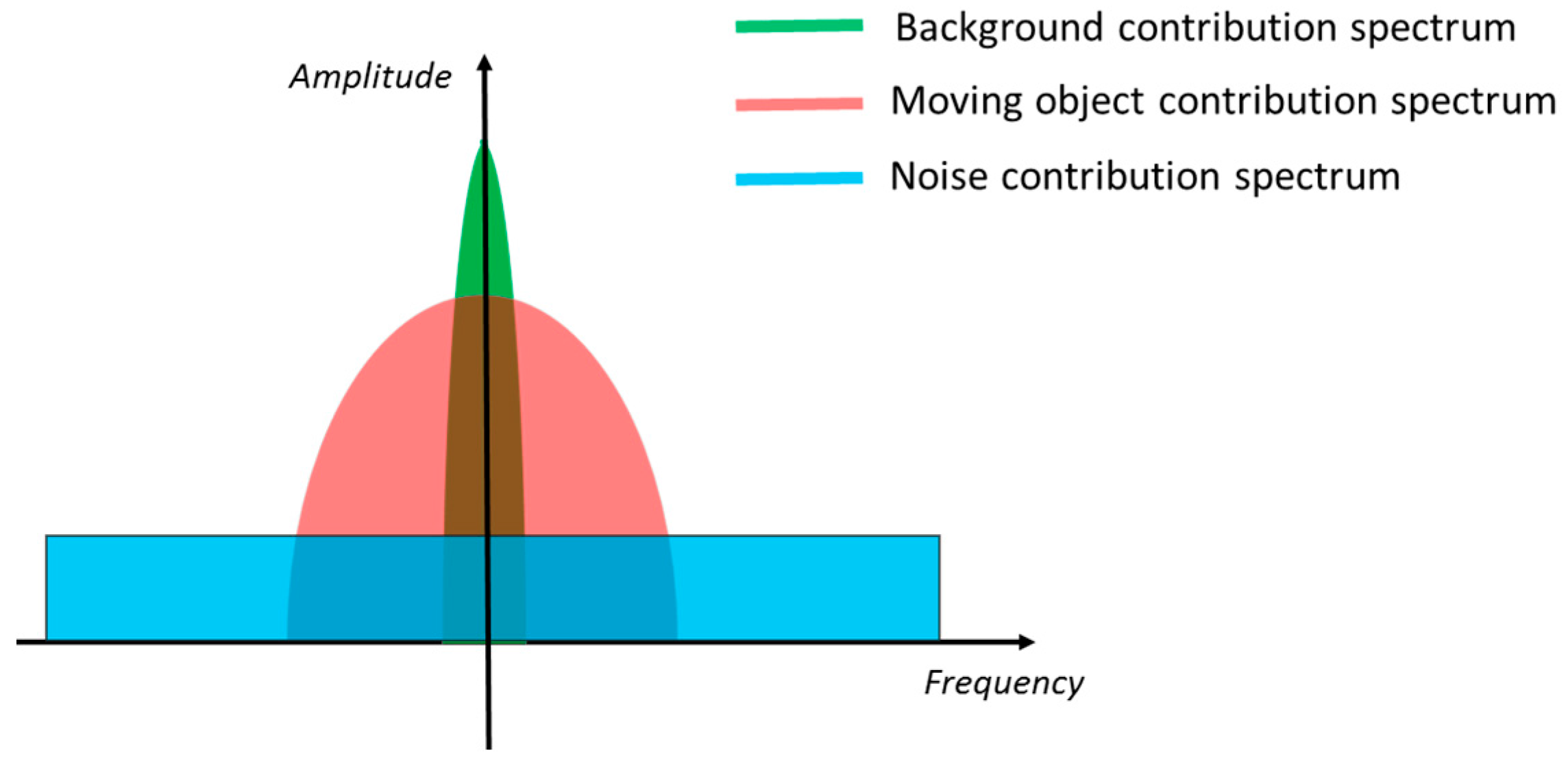
From the above considerations, it is reasonable to assume that the three contributions are quite distinct in the frequency domain, as schematically depicted in Figure 1. In fact, is located near zero frequency, whereas mostly spreads over low-medium frequencies (depending on the object velocity) and , being white, is the only contribution at high frequencies. Therefore, in principle, it is possible to separate each contribution by properly filtering along the time dimension, in order to extract the desired . Intuitively, through a low-pass filter, the noise contribution can be rejected, so that only the background contribution (in the case hypothesis occurs) or the moving object contribution (in the case hypothesis occurs) are left. Then, through a high-pass filter, also the background contribution can be eliminated, so that to have no contribution if occurs and only the moving object contribution if occurs, which means to detect the presence of moving objects.
However, it should be noted that the spectra of the three contributions are partially overlapped. Thus, if the overlap between and the other two components is large, a correct extraction of the moving objects is not possible by simply filtering out background and noise. A large overlap between and occurs when the velocity of a moving object is so high to generate significant high frequencies components in the spectra of . In fact, in this case, the two contributions have significant components at both the low and the high frequencies. (Note that not only the velocity, but also the size and the texture of the moving object influence the bandwidth of . In fact, a fast but large and not texturized object makes the pixels interested by its transit to maintain more less the same intensity for a long period, as if a slow object is passing. Analogously, a not too fast but small object has the effect of a fast object on the pixels where it passes.) Since it is asked to the proposed algorithm to detect also fast objects, the use a low-pass filter to extract the desired is not possible. A large overlap between and , instead, can be experienced because of drift phenomena of the measured intensity that could occur in electro-optical devices. For example, the response of the photodetectors in uncooled IR cameras is influenced by the changes of the internal temperature of the device, which results in undesired modifications of the actual pixel intensity over time [32]. Such drifts are in general more rapid than the changes of the background, thus they make the bandwidth of to increase more than expected. This is likely to generate great overlap between and in the presence of slow objects, whose contribution has narrow bandwidth, making a clear separation of their spectra impossible to perform with a simple high-pass filter.
Summarizing the concepts expressed in this section, it is possible to outline a method to properly tackle the problem in exam. First, a strategy to prevent or compensate the possible drifts of the IR camera should be applied to the video sequence, so as to reduce the bandwidth of and decrease the overlap with the bandwidth of . Then, working on each pixel singularly over time, the video sequence can be high-pass filtered, to remove . Finally, the separation between and can be obtained by exploiting only the statistical properties of the two contributions, so as to avoid using a low-pass filter and prevent the above-mentioned drawbacks. Possible refinements of the detection results should be performed only after has been discriminated from the other two contributions.
3. Proposed Solution
The proposed algorithm has been implemented from the considerations made in Section 2. It takes an IR video sequence as input and gives as output a map showing the position of the detected moving objects within each frame (detection map). To meet the requirement of working in real-time, the detection map of any frame is produced before the next one has been read. A brief overview of the algorithm functioning is presented below, whereas a detailed description of its single steps is reported in the next sections.
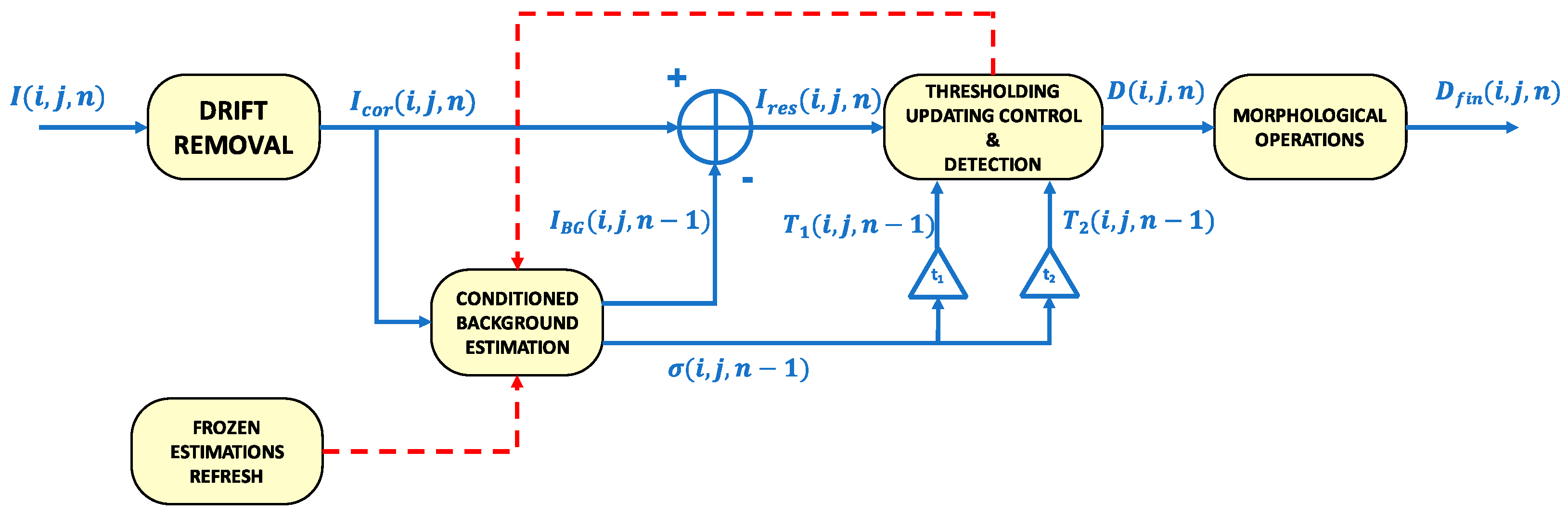
After a pre-processing phase aimed at correcting the possible drifts present in the video sequence, an estimation of the background, robust to global intensity changes, is computed pixel-by-pixel and updated frame by frame by means of a controlled first order infinite impulse response (IIR) filter. The control of the filter allows the background estimation not to be biased by the transit of an object. Then, the estimated background is subtracted to the original frame and each pixel of the residual image is processed through two thresholding stages. The first one provides the input to control the IIR filter. The second one permits discriminating the moving objects from the false alarms due to noise, leading to the generation of the detection map. The thresholds used in the two stages are calculated by means of another controlled IIR filter. This performs an estimation of the power of the noise frame by frame, allowing the thresholds to adapt to it. Again, the control of the filter avoids biased estimations due to the transit of an object. A final post-processing phase permits the detection map to be refined through some morphological operations, such as joining different parts of the same object and eliminating residual false alarms. The block diagram of the algorithm is depicted in Figure 2.
3.1. Prevention of Drifts of the Video Sequence Intensity
In Section 2, it has been pointed out how potential drifts of the intensity of the video sequence, due to technical limits of IR imaging devices, could make the spectrum of to overlap greatly with the spectrum of , impeding a clear separation of the two contributions. Such drift phenomena affect each frame uniformly over space [32], thus they can be modeled as an additive parameter to the video sequence intensity, variable over time and constant over space.
In order to remove its effects, the spatial average of the intensity, , is calculated over all the pixels of each acquired frame as
where and are, respectively, the number of rows and columns of the video sequence frames. Then, is subtracted from each pixel of , obtaining an image, , which will be referred to as corrected image or, in general, as corrected video sequence, no longer affected by the drift problem. It is worth noting that, after this operation, the intensity value of the pixels loses any physical meaning ( could even be negative). However, the relative value among different pixels, which is the quantity of interest, remains the same.
3.2. Background Estimation and Removal
Once a video sequence not affected by drift phenomena has been obtained, it is possible to remove the background contribution by exploiting the separation between its spectrum and the moving object spectrum. Thus first, for each pixel, , is low-pass filtered over time, in order to estimate the background contribution. Then, the result is subtracted from , obtaining the global effect of high-pass filtering the corrected video sequence.
The background estimation filter is implemented by means of an IIR filter, using an approach similar to [29]. Starting from the estimation at the -th iteration, , each pixel of the background is updated frame by frame utilizing the recursive rule
where the parameter , which assumes values between 0 and 1, controls the effective length of the impulse response of the filter or, equivalently, its bandwidth. In fact, by increasing , the effective number of previously acquired frames used to estimate the background increases and, thus, the incoming frame weighs less on the estimation. This is equivalent to reduce the bandwidth of the filter. Vice versa, by decreasing , the effective number of frames used to estimate the background decreases and weights more on the new estimation, which is equivalent to enlarge the bandwidth of the filter. The possibility to tune the bandwidth of the filter through the parameter allows the algorithm to be adjusted to the expected variability of the background, ensuring flexibility to different scenarios.
In general, should assume values close to the unity, since the background contribution has a very narrow bandwidth. The proper value of should be chosen by relating the effective length of the filter impulse response to the expected rapidity of the changes in the background. Several methods have been proposed to make such a choice [33,34,35]. In [35], authors suggest the following formula to relate to the effective length, , of the impulse response of a first order IIR filter:
where is the fraction of energy associated to the first samples. Then, setting to the value of the time interval in which the background is almost stationary and does not undergo considerable changes, can be computed accordingly, using Equation (4). If, for example, = 150 frames, then .
The proposed background estimation filter is both easy-to-implement and effective in terms of time consumption and memory allocation. In fact, at each step, only two multiplications for a constant and one sum of two matrices are performed, resulting in linear time-complexity. In addition, data storage is limited to one matrix per frame, since only the estimation of the background at the previous step needs to be saved.
Using a linear filter instead of a nonlinear one is crucial for the algorithm to fit the real-time requirement without adopting expensive hardware. In fact, typical nonlinear filters for background estimation, such as the median [28] and the min–max [36], need to sort the values that each pixel assumes at every acquired frame, resulting in quadratic time-complexity. However, nonlinear filters permit intensity peaks, which occur for example when an object passes in a specific pixel, to be removed from the estimation of the background, so as not to bias the background estimation. Instead, the used filter is not capable to deal with this situation, resulting in possible missing detections. In order to solve this problem a control strategy is implemented in the filter. It works by stopping the updating of for those pixels whose amplitude deviates from the previous estimation more than a certain threshold. Then, when the amplitude drops again below the threshold, the updating restarts. (It is worth noting that the updating control strategy makes the filter to become nonlinear. However, its computational efficiency is practically the same of a linear filter.) The strategy can be expressed in formula as
In Equation (5), is the threshold, which is calculated frame by frame and for each pixel as
where is the standard deviation of —whose calculation is object of Section 3.3—and is a parameter tunable by the user. From the model in Equation (1), if the hypothesis is verified then is given by the sum of and . Considering that is almost constant in limited time intervals, then the time variability of is mostly due to the contribution. Thus, is a good approximation of the standard deviation of the noise. Being a function of , then the threshold is adaptive to the noise, ensuring robustness against it. The parameter allows tuning the control of the filter, so as to make the user free to decide whether to tolerate more the transit of low-contrasted moving objects (higher values of ) or the noise (lower values of ), depending on the specific application.
After estimating the background contribution at frame , the result is subtracted from the next incoming frame, previously corrected, . A residual image, , is obtained, which is expected to contain only the contributions of the noise ( hypothesis) or the contribution of both the moving objects and the noise ( hypothesis).
Initialization of the Background Estimation Filter
The background estimation filter needs to be initialized, namely the value should be found. The most intuitive initialization method is to use the first acquired frame as the initial background estimation [29]. However, this method is too prone to the presence of noise, thus it is likely to generate inaccurate estimations, especially in the first iterations. To overcome this problem, a more robust calculation of is performed by integrating the information of more frames together. This is done by averaging the first acquired frames pixel by pixel over time, namely
where the index refers to the frames acquired before beginning to run the controlled filtering in Equation (5). should be increased as the SNR of the video sequence images decreases. In practical cases, setting it to some tens (i.e., 30 or 40 frames) should ensure a robust estimation. In order to avoid storing images, which would violate the requirement of low memory allocation, Equation (7) is calculated recursively, by adding the last acquired frame to the sum of the previous ones and storing only the result of this operation at each step. Thus, the same memory necessary to store a single image is occupied.
To avoid possible bias of , no objects should pass through the scene during the first frames are being acquired. However, in the unfortunate case in which a moving object crosses the scene in this time interval, the strategy that allows refreshing the frozen estimations, explained in Section 3.5, ensures a new correct background estimation after a few frames.
3.3. Estimation of the Standard Deviation of Noise
As seen in Section 3.2, the standard deviation, , of is a good approximation of the standard deviation of the noise, which has to be estimated in order to calculate in Equation (7). The estimation of , is performed similarly to the estimation of the background that is, using a first order IIR filter, as in Equation (3). Actually, not directly but the variance of , , is estimated. This allows using a linear filter instead of a nonlinear one. can then be obtained by simply computing the square root of . Hence, starting from the estimation at the -th iteration, the variance of each pixels is updated frame by frame through
where , which assumes values between 0 and 1, plays the same role of in Equation (3), namely it allows controlling the rapidity of the updating by increasing (lower values of ) or decreasing (higher values of ) the bandwidth of the filter. Like , also is expected to vary slowly, since it depends on the power of the noise process, which suffers slight variations in the presence of background intensity changes, due to the shot noise phenomenon [37]. Thus, as , also should assume values close to 1. Similar considerations to those made in Section 3.2 for the choice of can be made also for .
The estimation of is also likely to be biased by the transit of a moving object in the pixel . This results in wrongly estimated values of , which can affect the updating control of in Equation (5). Therefore, the control strategy in Equation (5) is applied also to the estimation of in Equation (8):
The updating of is thus performed only when does not deviate significantly from the estimated background value (absence of moving objects), and interrupted otherwise (presence of a moving object).
Initialization of the Variance Estimation Filter
As for the background estimation filter, the variance estimation filter also needs to be initialized. Again, to avoid results corrupted by the noise, a robust calculation of the initial variance, , based on the integration of the information relative to more frames, is preferred instead of using only the first acquired frame. Thus, is derived through the formula:
where the index refers to the frames acquired before beginning to run the controlled filtering in Equation (9), is the same number of frames used to calculate in Equation (7) and is the average of the pixel calculated over the first frames, which can be directly taken from the -th step of the recursive procedure for estimating . To avoid storing matrices, also Equation (10) is calculated recursively.
3.4. Adaptive Thresholding Detection
As said in Section 3.2, the residual image after background removal, , is composed by the contribution of the noise solely, if hypothesis is verified, and by the contribution of the noise added to that of the moving objects, if hypothesis is verified instead. In Section 2, it has been pointed out that, even if, in general, the spectra of and should be separable, this hypothesis may be wrong in the presence of fast and/or small objects. For this reason, low-pass filtering to isolate , is not advisable.
Thus, an alternative strategy has been implemented. It consists in comparing the absolute value of with a threshold, calculated for each pixel and updated frame by frame, which depends on the power of the noise. If is lower than the threshold, this is probably due to the absence of moving objects, since the residual intensity is composed only by the noise ( hypothesis), which slightly variates around zero. Instead, if exceeds the threshold, this is probably due to the presence of a moving object ( hypothesis), whose intensity is added to the noise contribution, making the total intensity to increase. The decision strategy can be expressed as
where is the threshold for the pixel , calculated after frames have been acquired, by using the equation:
where is a parameter tunable by the user and is the standard deviation of , calculated and updated as in Equation (9). As , also is a function of and, thus, it is adaptive to the noise. The possibility to tune allows the user to decide the behavior of the algorithm in terms of sensitivity to dim objects and false alarm rate, so as to be suitable for different applications and different scenarios. In fact, setting to lower values permits tolerating a higher false alarm rate, due to the peaks of noise, in order to improve the capability of detecting poorly-contrasted objects. Vice versa, setting to higher values permits decreasing the sensitivity to dim objects in order to limit the false alarms. It is worth noting that the two thresholds used for the controlled filters Equations (5) and (9), respectively, differ for a scale parameter ( in Equation (5) and in Equation (9)). The choice of using different thresholds, instead of the same one for the two control routines, has been made because the presence of peaks of noise that exceed the threshold is more critical in Equation (9) than in Equation (5). In fact, if the threshold is exceeded for one frame, only an undesired stop of the background estimation updating occurs, which is likely to be irrelevant on the global calculation. Conversely, when the threshold is exceeded, a wrong detection is reported. For this reason, should be higher than that is .
The output of the thresholding operation in (11) is a binary map, , that shows which pixels contains a moving object or a part of it in the -th frame () and which not (). Actually, is just a rough detection map, which needs to be refined to be better interpreted, as shown in Section 3.6.
3.5. Refresh of the Frozen Estimations
The control strategy applied in Equations (5) and (9) has a major drawback. If a steady object present within the scene begins to move and leaves its initial position, significant deviations of from the background intensity value are expected both for the pixels currently occupied and for the pixels initially occupied by the object. This results in high values of which are likely to exceed the threshold in Equation (11) and, hence, to make a detection to be reported. While this behavior is the one desired for the pixels currently occupied by the object, it is undesired for the pixels initially occupied, where the intensity of the object is misinterpreted as the one of the background and, consequently, the real background is detected as a moving object. Moreover, considering that the quantity in Equations (5) and (9) is equivalent to , and that should be higher than , as said in Section 3.4, the update of the estimations of and is likely to be stopped. Thus, the erroneous estimation of the background does not change, making the problem of the wrong detection to persist indefinitely.
To avoid the freezing of the estimations, another control is applied to Equations (5) and (9). It works by deleting the values of and for those pixels for which has not updated in the last frames, and by calculating new estimations through Equations (7) and (10). Such estimations will then be updated normally, by using Equations (5) and (9). Considering that is the number of frame necessary to calculate the initial estimations (see Section 3.2.1), frame are needed, in total, to restore the regular functioning of the filters. The parameter can be choose by the user according with the minimum velocity of the objects to be detected. If such velocity is pixels per frame, then
To avoid imposing a limit to the minimum velocity of the objects, allowing more flexibility, the quantity can be set close to the expected rapidity of the background changes measured in frames, , so as to be constrained only by physical limits. As an example, referring to the calculation of made in Section 3.2 in which it has been supposed that , setting (Section 3.2.1) and subtracting a margin of error of 75 frames, from Equation (13) we obtain .
3.6. Refinement of the Detection Map
The last stage of the algorithm consists in refining the binary map, , in order to obtain the final detection map, . This is performed through some morphological operation. The first operation is optional and consists in eliminating all the single-pixel isolated detections that is, to set to zero the pixels of equal to one and surrounded by pixel all equal to zero. If performed, it permits the false alarm rate to decrease strongly, since, being the noise process independent for each pixel, the probability of having more than one false alarm in a 3-pixels side square region around is in the order of the square of the probability of having a false alarm in one single pixel. This operation is left as optional since it could be required to detect also single-pixel objects, which would be eliminated otherwise.
The second operation consists in a sequential application of a dilation followed by an erosion [38]. It permits joining different connected groups of pixels (blobs) equal to one that are close to each other. This operation is particularly useful in the presence of a non-uniform moving object, since only some parts of it may be successfully detected, resulting in separated blobs in the detection map that could be mistaken for several different objects. Joining these blobs together should make the detected object to be a single body, also helping to recognize its shape.
4. Results and Discussion
An experimental analysis has been carried out to verify the effectiveness of the proposed algorithm on the cases listed in Table 1, and to compare it with other commonly used moving object detection algorithms. For this purpose, a database of 24 IR video sequences has been created. The main specifications of the IR camera employed to acquire the video sequences are reported in Table 2. The video sequences contain 13 small objects and 11 large objects with different sizes, 18 dim objects with different contrasts with respect to the background, 12 fast objects and 12 slow objects with different velocities and 7 objects that change their trajectory (some objects have more than one of these characteristics at the same time). In 10 video sequences multiple objects are present. An accurate ground truth has been constructed for each video sequence, by both planning and controlling the movements of the objects while crossing the scene and by visual inspecting the acquired videos.
The algorithm assessment has been carried out for each different kind of moving objects singularly, by considering only the video sequences in which they appear. Then, also the global performance has been evaluated. Three performance indexes have been used for the assessment. First, the object detection rate, , intended as the number of frames in which the moving objects have been correctly detected over the total number of frames. An object is declared as detected if at least one of its pixels is detected. Second, the pixel detection rate, , intended as the percentage of detected pixels of each moving object in each frame, given a correct detection, averaged over the total number of moving objects and over the total number of frames. has been expressed in percentage to distinguish it more clearly from , which is expressed in decimals instead. Note that gives an idea of the capability of the algorithm to return the correct shape of the detected objects, since high values of indicate that most of the object pixels have been properly detected. Third, the false alarm rate, , calculated as the number of pixels in which a false alarm is reported over the total number of pixel of all the frames considered together. In addition to these three indexes, the computational time, , defined as the average time needed for the algorithm to run a single iteration, has also been measured to evaluate if the real-time requirement can be achieved even using low cost hardware.
The performance of the proposed algorithm has been compared against other three algorithms, which implement some of the most commonly adopted DBT strategies. The considered approaches are the one described in [21], which is a refined version of frame differencing (let us indicate it as FD for the sake of brevity), the GMM-based approach described in [25] (indicated here as GMM), and an approach based on the median filter applied to each pixel singularly over time, and speeded-up as in [28] (indicated as MED). Each of these algorithms has been properly tuned according with the expected characteristics of the moving objects present in the considered video sequence. The same has been done with the proposed algorithm, by adjusting the parameters, in Equation (5), in Equation (6), in Equation (9) and in Equation (12), following the guidelines exposed in Section 3.2, Section 3.3 and Section 3.4. However, in order to recreate a more realistic situation and also to evaluate the flexibility of the algorithms to adapt to different cases, the exact size, contrast and velocity of the moving objects have been considered as unknown. Thus, the tuning has been made only on the expected qualities of the moving objects, without relying on actual quantities.
4.1. Algorithm Assessment in the Presence of Small Objects
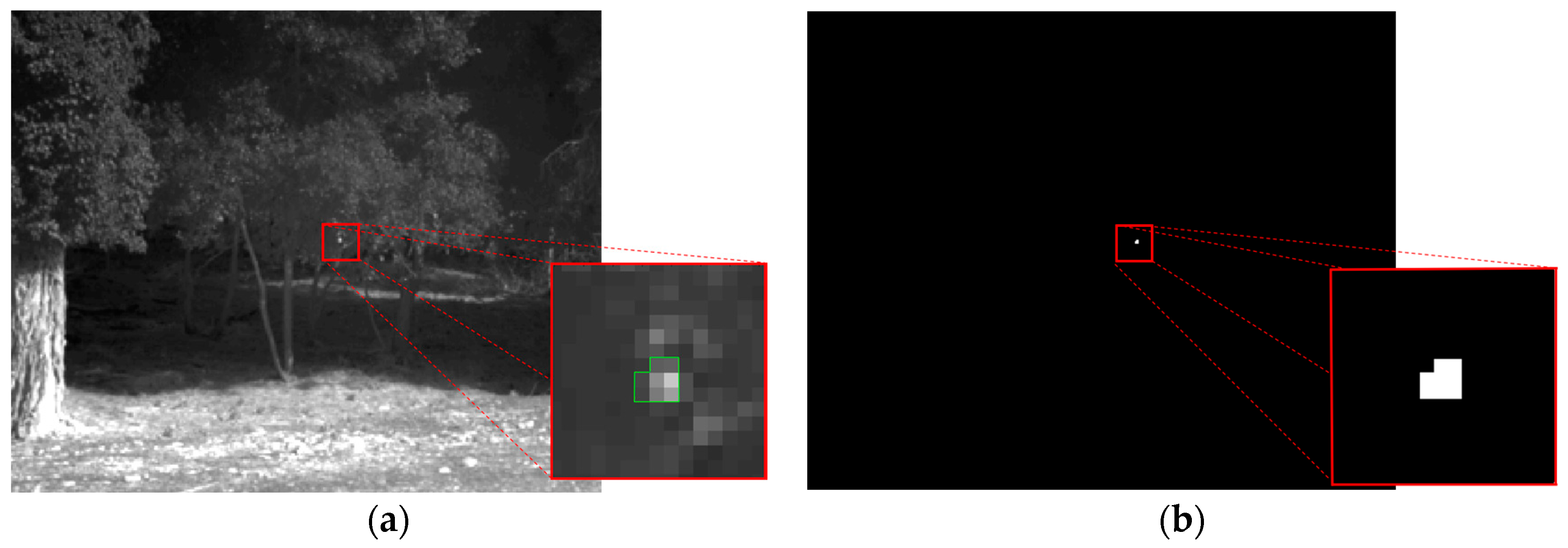
Small objects have been defined as objects covering an area between 1 and 16 pixels within a frame. The video sequences containing such kind of objects have been analyzed jointly to assess the performance of the proposed algorithm in the presence of small moving objects. Figure 3a shows an example frame of one of such video sequences. It contains a little stone, hotter than the background, which has been thrown from a side of the scene to the other. The stone occupies 8 pixels, thus it can be considered as a small moving object (due to its average velocity of 16 pixels per frame, the stone can be also considered as a fast object, as it will be explained in Section 4.5). In the zoomed box, the object is highlighted with a green line contouring its shape for better clarity. The detection map output by the proposed algorithm at the considered frame is shown in Figure 3b, with a zoom of the region containing the detected pixels. A comparison between the video sequence frame and the detection map clearly reveals the effectiveness of the algorithm, which has been capable to detect correctly all the pixels belonging to the moving objects. In addition, no false alarms are present.
The three performance indexes described in Section 4 has been calculated over all the video sequences containing small moving objects. The obtained object detection rate and pixel detection rate, which are generally the most critical parameters when dealing with small objects are, respectively, and . Such a result confirms that the algorithm is able to detect moving objects with small size successfully. Good results have been achieved also in terms of false alarm rate, which is . In fact, considering that the camera resolution is 640 × 512 pixels, this means that more or less 0.062 false alarms per frame are expected that is, about one single-pixel false alarm every 16 frames.
4.2. Algorithm Assessment in the Presence of Large Objects
Large objects have been defined as objects covering an area wider than 2500 pixels with at least 10 pixels in the smallest dimension (namely 10 × 250 pixels or higher in both dimensions), and occupying more than 1/100 of the frame size. In Figure 4a, an example frame of a video sequence containing a large moving object is presented. It consists in a van that is approaching the camera. The corresponding detection map produced by the proposed algorithm is shown in Figure 4b. The goodness of the result stands out clearly by noting that it is possible to guess the shape of the vehicle directly by looking at the map, since the detection has been successfully performed even for the details, such as the wheels and the rearview mirrors.
The three chosen indexes of performance have been calculated over all the video sequences containing large moving objects, confirming the effectiveness of the algorithm in dealing also with this situation: , and . In particular, whereas a high value of was expected, since large objects are composed by many pixels and just detecting one of them results in a correct detection, the index could have been critical, since, as seen in Section 1, large objects are prone to the self-deletion problem. Nevertheless, the algorithm has performed very well also in terms of , with an average percentage higher than 95% of correctly detected pixels of each object. The false alarm rate is similar to the one obtained in the case of small objects.
4.3. Algorithm Assessment in the Presence of Dim Objects
The behavior of the algorithm in the presence of dim moving objects has been evaluated by computing the three performance indexes over all the video sequences containing moving objects whose contrast with respect to the background is lower than 1% of the dynamic range of the considered frames, calculated when no moving objects are present. The following definition has been adopted for the contrast:
where is the group of pixels occupied by the moving object at the frame and by the background at the frame , and is the number of pixels of such a group. The obtained results are , and . With respect to the cases in which more highly-contrasted objects are present, the two detection rate indexes are lower, especially . This was expected, since the intensity values of the moving objects are close to the threshold and, thus, are likely to drop below it because of noise peaks and blurring effect, resulting in missed detections. Despite this, the achieved performance is reasonably good, as the objects has been correctly detected in more than 90% of the frames and for more than 80% of their area, in average. The slightly higher false alarm rate can be explained by the lower values chosen for and, mainly, , which have been decreased to permit dim objects to be detected. However, the result is still tolerable, considering that less than 0.1 false alarms per frame are expected.
Figure 5a reports an example frame containing two moving objects, namely a person and a little truck, covered with a tarpaulin with low emissivity, passing close and away from the camera, respectively. The truck is a dim object, as visible in the zoomed box (green contour), where it is indistinguishable from the background. Despite this, it has been successfully detected as well as the person walking, as the detection map of the considered frame shows in Figure 5b. It is worth noting that, even if not all of the pixels belonging to the dim object are detected, especially the edge ones due to blurring effects, the percentage of detected pixels is sufficient to guess the shape of a vehicle.
4.4. Algorithm Assessment in the Presence of Fast Objects
Fast moving objects has been defined as objects with a higher velocity than 10 pixels per frame. An example frame of a video sequence in which a fast object is present has been shown previously in Figure 3a, jointly with the corresponding detection map (Figure 3b). In such an example, indeed, the object moves at about 16 pixels per frame.
The performance indexes obtained in the presence of fast moving objects are , and . Even in this case, promising results have been obtained in terms of both detection and false alarm rate.
4.5. Algorithm Assessment in the Presence of Slow Objects
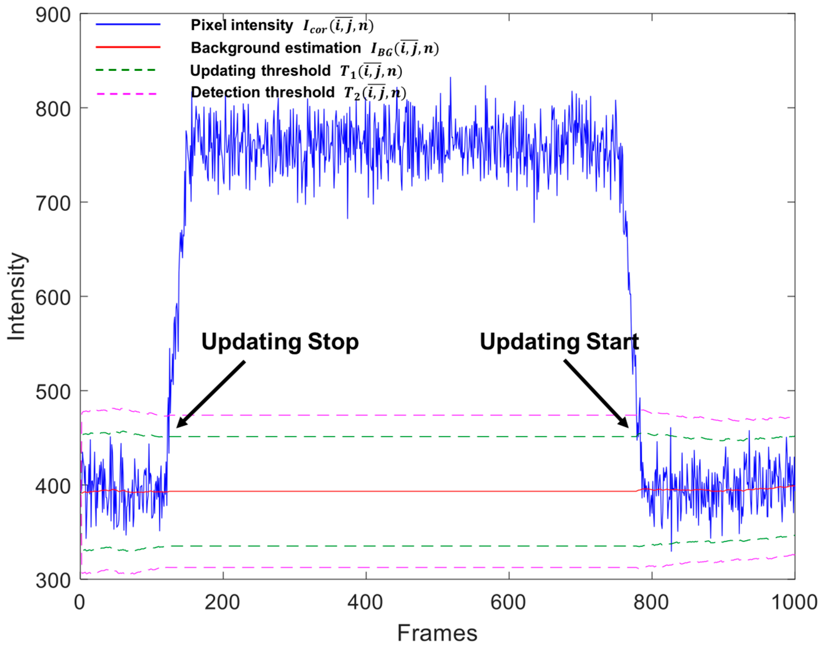
An object has been defined as slow if it moves at a velocity lower than 0.08 pixels per frames, namely one pixel every half a second, considering the 25 Hz camera frame rate. Figure 6a shows an example frame of a video sequence in which a terrestrial rescue vehicle, partially covered by a small dip of the road, is crossing the scene far from the camera at about 0.015 pixels per frame. The vehicle is pointed out by a green contour in the zoomed box. Since its velocity is lower than 0.08 pixels per frame it is considered as slow. The detection map output by the algorithm at the selected frame, shown in Figure 6b, reports a correct detection of all the pixels belonging to the moving object. To better show the algorithm functioning, it is meaningful to report the plot over time of the intensity of a pixel crossed by the moving object, after the removal of (Equation (2)), jointly with the background estimation, , and the two thresholds, and , (Figure 7). The transit of the object through the considered pixel occurs between frames 122 and 784, as it is evident from the increase of the intensity. As soon as this overcomes , the background and standard deviation estimation are halted (Equations (5) and (9)). Thus, the updating of , and (which depend on ) stops, as revealed by the flatness of the curves of such quantities in the frame interval in which the object is passing. This permits the estimations not to be biased by the intensity of the moving object.
The capability of the algorithm to detect slow objects is proven by the performance indexes, which are , and . It is worth noting that is slightly lower than in the previous cases. This because, in a pixel affected by the transit of the target, the transition of the intensity from the background to the object level is slow, thus it takes some more for the intensity to overcome , resulting in some missing detections. The false alarm rate is in line with the other cases.
4.6. Algorithm Assessment in the Presence of Objects That Change Their Trajectory
The presence of moving objects that change their trajectory while crossing the scene generally affects those strategies based on spatial-temporal analysis, such as TDB ones. Since the proposed algorithm is based on a DBT strategy, which does not require any assumption about the object path and velocity, it is not expected to be affected by this issue. Indeed, the results obtained by running the algorithm on the 7 video sequences that contains trajectory changing objects demonstrate its effectiveness: , and .
4.7. Algorithm Assessment in the Presence of Multiple Objects
The last case study concerns the contemporary presence of more than one moving object in the scene, as it occurs, for example, in the frame shown in Figure 5a. To assess the capability of the proposed algorithm to deal with this situation, the performance indexes have been calculated over the 10 video sequences in which multiple objects are present. The obtained results again demonstrate the effectiveness of the algorithm, both in terms of high detection rate ( and ) and in terms of low false alarm rate ().
4.8. Global Assessment of the Proposed Algorithm
The global performances of the algorithm have been calculated by computing the three indexes over all of the video sequences. The global detection rate of the proposed algorithm is , with a maximum of 0.997 for the case of large objects and a minimum of 0.922 for the case of slow objects. Such a result proves the capability of the algorithm to detect moving objects in all the challenging situations typical of the addressed issue. A further proof of the effectiveness of the algorithm is given by the percentage of correctly detected pixels of the moving objects, which is 91.8% in average. This should allow a user to recognize the shape of the detected objects by directly looking at the detection map. The algorithm is also robust to false alarms, whose rate is approximately the same in every case and, globally, it is . At the resolution of the employed camera, this means that about one single false alarm every 14 frames is expected.
Finally, the average time needed for the algorithm to perform a single iteration has been calculated over all the frames of all the video sequences to verify if the real-time requirement is satisfied. As mentioned in Section 3, we consider the real-time performance achieved if the output of a single iteration—namely, the detection map of a single frame—is produced in less than 1/25 s, which is the typical frame rate of a low-cost video acquisition system and also the one of the used camera. Such a condition ensures that the detection map at a certain frame is produced before the successive frame is acquired. The algorithm has been run on a commercial low-cost hardware, consisting in a 1.7 GHz CPU board and a 4 GB RAM. An average time per iteration ms has been obtained, which is less than half the maximum tolerated value. Thus, the algorithm is compliant with the real-time requirement.
For the sake of clarity, all the results obtained by running the proposed algorithm are summarized in the first column of Table 3. These have been compared with the results obtained by running the three detection algorithms mentioned in Section 4, both considering each different kind of moving object singularly (the cases of objects that change their trajectory and multiple objects have been omitted in Table 3, since they are less significant for a comparison among DBT algorithm exploiting temporal domain, which are generally not affected by such issues) and all the objects together. Such results are also reported in Table 3, where, in addition, the top performance among the four algorithms has been highlighted, for each index and for each different kind of object. At a global level, the proposed algorithm outperforms the other three, except for the index . The FD algorithm, in fact, runs about three time faster. However, it demonstrates to perform poorly concerning the other three indexes, in particular for and . The former index suffers the presence of objects less hot than the background, which cannot be detected at all. The second, instead, is strongly affected by the self-deletion problem. In fact, in the presence of large and slow object, for which the problem is more critical, and 58.4%, respectively; that is, only about half of the pixels of the objects are detected. The MED algorithm performs similarly to the proposed algorithm in terms of detection rate, even achieving better results in the presence of small and fast objects. However, its computational time is dramatically high, being the global more than 15 times greater than the time required by the proposed algorithm and more than 6 time greater the maximum tolerated value. Thus, the MED algorithm is not suitable for real-time applications. The problem is particularly critical in the presence of large and slow objects, since more frames must be buffered to allow the median of the intensity to be equal to the background intensity and not to the object one, for those pixels interested by the transit of an object. In these cases, to limit , a lower number of stored frames should be chosen. Unfortunately, for the reason just now mentioned, this is likely to produce an estimation of the background intensity equal to the object one, resulting in missing detections, as the low values of and mainly in the presence of large and slow objects demonstrates. Moreover, artifacts are likely to appear in those pixels where an object is passed a few frames before, making the false alarm rate to increase ( and 11.73 × 10⁻⁷ for the large and slow objects cases, respectively). The GMM algorithm not only performs slightly worse than the proposed algorithm in terms of , and , but also has a global ms that is, a bit higher than the maximum tolerable value to work in real-time. Summarizing the results of the comparison, it is possible to state that the proposed algorithm is more capable to deal with challenging moving objects than the other algorithms, showing a greater flexibility to different situations, while ensuring the real-time performance also when low-cost hardware is utilized.
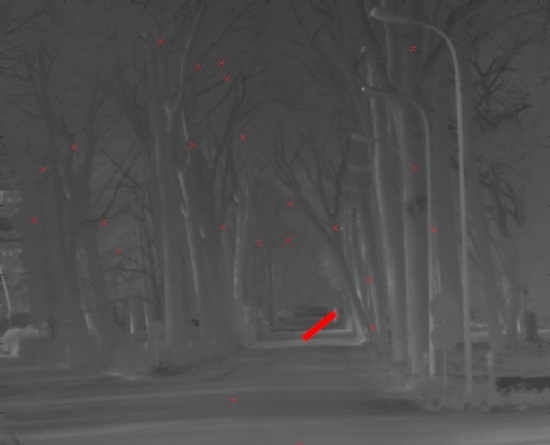
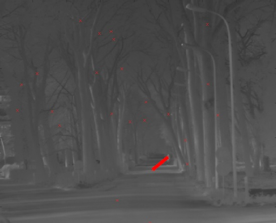
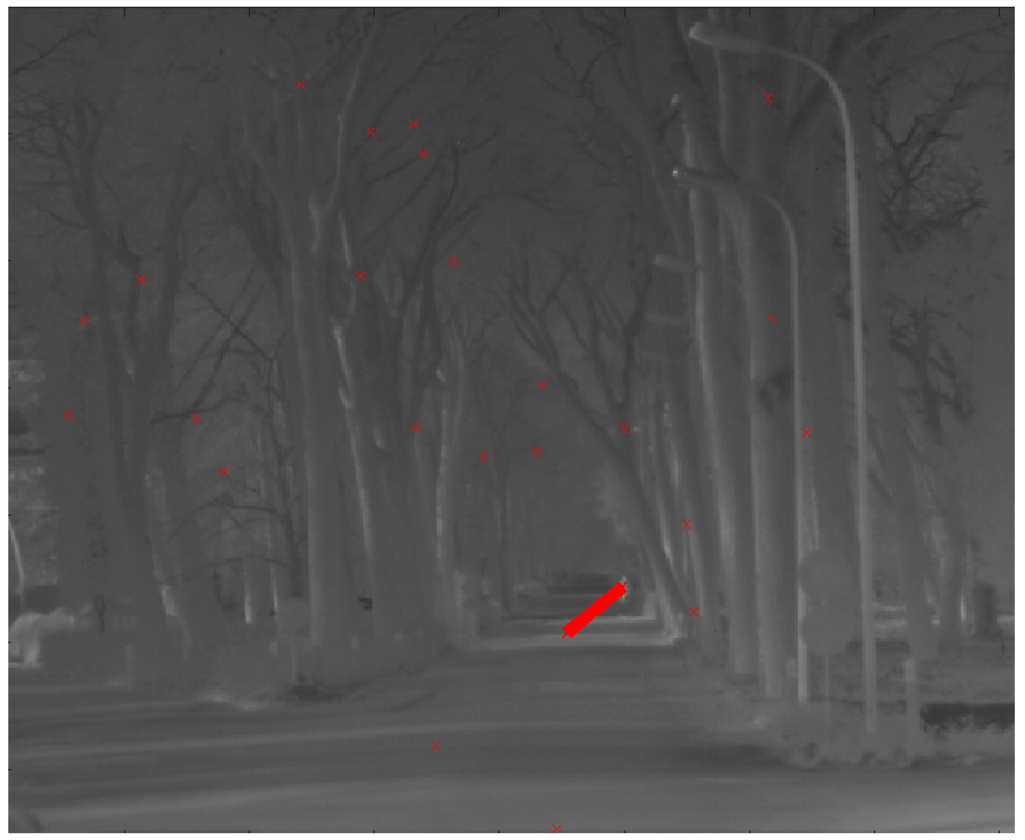
As a final assessment, all the detections reported in one of the video sequences of the dataset have been plotted on a frame chosen as reference (a marker has been placed on the centroid of each detected blob in each frame). The result is shown in Figure 8. The presence of a moving object is clearly visible from the trail left by the markers, which also proves the detection capability of the algorithm. Such an example suggests that the algorithm can be profitably employed as a first stage of a tracking system. In fact, the reported positions of the objects detected by it can be used to feed a tracker, which should simply calculate the spatial-temporal correlation among them in order to extract their tracks. In the reference frame, a few false alarms have been reported, which are represented by the isolated markers. Their presence does not affect the final result significantly, proving that the obtained false alarm rate is low enough.
5. Conclusions
We presented an algorithm for automatically detecting moving objects in video sequences acquired with IR steady cameras, designed with the purpose of dealing with different challenging situations, typical of this task, such as the presence of small, large, dim, fast and slow objects, multiple objects and objects that change their trajectory. Furthermore, the constraints of working in real-time on cheap hardware and avoiding occupying a great amount of memory have been imposed.
The algorithm has been tested on a database of IR video sequences that contains all the above-mentioned kinds of moving objects, demonstrating to be very effective both globally and against each different kind of object. An overall detection rate higher than 96% has been achieved against a false alarm rate of 2.21 × 10⁻⁷, which means that only a single false alarm every 14 frames is likely to occur. Furthermore, 91.8% of the pixels of the moving objects have been correctly detected on average, allowing one to guess the shape of the detected objects directly from the detection map. Even in the most critical cases, the algorithm has shown reasonably good performances. The minimum object detection is 92.2% (in the presence of slow objects), whereas the minimum percentage of detected pixel per object is 83.1% and the maximum false alarm rate is 2.81 × 10⁻⁷ (in the presence of dim objects). The algorithm has also respected plenty the real-time requirement, being 17.5 ms the average time needed to run an iteration, which is less than half the typical camera frame rate of 1/25 s. This means that the detection map at a certain frame is output before the next frame is acquired. Compared against other commonly used moving detection algorithms, the proposed one has achieved better overall performances, showing a greater flexibility to different situations.
Given its reliability and flexibility, the algorithm can be successfully employed in a wide variety of video-surveillance applications, such as intrusion monitoring, activity control and detection of approaching objects, especially when real-time processing is mandatory, as in the case of rescue or defense purposes. It can also be profitably used as a first stage of a detection and tracking system, since it provides the plot of the moving objects position independently of their size and velocity, which is a crucial information to feed a tracker with.
Acknowledgments
The authors would like to acknowledge the Electro-Optical Division of the CISAM, San Piero a Grado (PI), Italy, for the continuos support in our research activity.
Author Contributions
Andrea Zingoni, Marco Diani and Giovanni Corsini proposed the method; Andrea Zingoni designed, performed and analyzed the experimental tests; Andrea Zingoni wrote the paper and Marco Diani and Giovanni Corsini reviewed it and suggested some improvements.
Conflicts of Interest
The authors declare no conflict of interest.
References
- Huang, K.; Mao, X. Detectability of infrared small targets. Infrared Phys. Technol. 2010, 53, 208–217. [Google Scholar] [CrossRef]
- Reed, I.; Gagliardi, R.; Stotts, L. Optical moving target detection with 3-D matched filtering. IEEE Trans. Aerosp. Electron. Syst. 1988, 24, 327–336. [Google Scholar] [CrossRef]
- Bai, X.; Zhang, S.; Du, B.; Liu, Z.; Jin, T.; Xue, B.; Zhou, F. Survey on dim small target detection in clutter background: Wavelet, inter-frame and filter based algorithms. Procedia Eng. 2011, 15, 479–483. [Google Scholar] [CrossRef]
- Rozovskii, B.; Petrov, A. Optimal nonlinear filtering for track-before-detect in IR image sequences. In Proceedings of the SPIE: Signal and Data Processing of Small Targets, Denver, CO, USA, 20–22 July 1999. [Google Scholar]
- Porat, B.; Friedlander, B. A Frequency Domain Algorithm for Multiframe Detection and Estimation of Dim Targets. IEEE Trans. Pattern Anal. Mach. Intell. 1990, 12, 398–401. [Google Scholar] [CrossRef]
- Tursun, D.; Guiying, X.; Hamdulla, A. A Particle Filter Based Algorithm for State estimation of Dim Moving Point Target in IR Image Sequence. In Proceedings of the 2nd International Symposium on Intelligent Information Technology Application, Shanghai, China, 20–22 December 2008; Volume 2, pp. 127–131. [Google Scholar]
- Barniv, Y. Dynamic Programming Solution for Detection of Dim Moving Targets. IEEE Trans. Aerosp. Electron. Syst. 1985, 21, 144–156. [Google Scholar] [CrossRef]
- Pakfiliz, A.; Efe, M. Multi-Target Tracking In Clutter with Histogram Probabilistic Multi-Hypothesis Tracker. In Proceedings of the 18th International Conference on Systems Engineering, Las Vegas, NV, USA, 16–18 August 2005; pp. 137–142. [Google Scholar]
- Hamdulla, A.; Lian, X. High-resolution Bayes Detection of Dim Moving Point Target in IR Image Sequence Using Probabilistic Data Association Filter. In Proceedings of the 2008 International Conference on Computer Science and Software Engineering, Wuhan, China, 12–14 December 2008; Volume 6, pp. 365–368. [Google Scholar]
- Moyer, L.; Spaak, J.; Lamanna, P. A Multi-Dimensional Hough Transform-Based Track-Before-Detect Technique for Detecting Weak Targets in Strong Clutter Backgrounds. IEEE Trans. Aerosp. Electron. Syst. 2011, 47, 3062–3068. [Google Scholar] [CrossRef]
- Davey, S. A Comparison of Detection Performance for Several Track-Before-Detect Algorithms. In Proceedings of the 11th International Conference on Information Fusion, Cologne, Germany, 30 June–3 July 2008; pp. 1–8. [Google Scholar]
- Mohan, A.; Papageorgiou, C.; Poggio, T. Example-Based Object Detection in Images by Components. IEEE Trans. Pattern Anal. Mach. Intell. 2001, 23, 349–361. [Google Scholar] [CrossRef]
- Wang, C.; Zhang, J.; Gu, Y. Small target extraction based on Independent Component Analysis for Hyperspectral imagery. Geo-Spat. Inf. Sci. 2006, 9, 103–107. [Google Scholar]
- Fakiris, E.; Papatheodorou, G.; Geraga, M.; Ferentinos, G. An Automatic Target Detection Algorithm for Swath Sonar Backscatter Imagery, Using Image Texture and Independent Component Analysis. Remote Sens. 2016, 8, 373. [Google Scholar] [CrossRef]
- Wiliams, D.P.; Fakiris, E. Exploiting Environmental Information for Improved Underwater Target Classification in Sonar Imagery. IEEE Trans. Geosci. Remote Sens. 2013, 52, 6248–6297. [Google Scholar] [CrossRef]
- Chen, Z.; Liu, C.; Chang, F. Infrared Small Target Detection Algorithm Based on Feature Salience. Int. J. Pattern Recognit. Artif. Intell. 2011, 25, 137–145. [Google Scholar] [CrossRef]
- Wang, X.; Lv, G.; Xu, L. Infrared Dim Target Detection Based on Visual Attention. Infrared Phys. Technol. 2012, 55, 513–521. [Google Scholar] [CrossRef]
- He, W.; Zhang, L. Dim Target Detection in Infrared Image Sequences Using Accumulated Information. Innov. Algorithms Tech. Autom. Ind. Electron. Telecommun. 2007, 493–496. [Google Scholar] [CrossRef]
- Zivkovic, Z. Improve Adaptive Gaussian Mixture Model for Background Subtraction. In Proceedings of the 17th International Conference on Pattern Recognition, Cambridge, UK, 23–26 August 2004; Volume 2, pp. 28–31. [Google Scholar]
- Lei, L.; Zhijian, H. Infrared Small Target Detection Technology Based on OpenCV. In Proceedings of the SPIE: Signal Processing, Sensor Fusion and Target Recognition XXII, Baltimore, MD, USA, 23 May 2013. [Google Scholar]
- Jihui, Y.; Yongjin, K.; Boohwan, L.; Jieun, K.; Byungin, C. Improved Small Target Detection for IR Point Target. In Proceedings of the 34th International Conference on Infrared, Millimeter, and Terahertz Waves (IRMMW-THz 2009), Busan, South Korea, 21–25 September 2009; pp. 1–2. [Google Scholar]
- Zhan, C.; Duan, X.; Xu, S.; Song, Z.; Luo, M. An Improved Moving Object Detection Algorithm Based on Frame Difference and Edge Detection. In Proceedings of the 4th International Conference on Image and Graphics (ICIG 2007), Sichuan, China, 22–24 August 2007; pp. 519–523. [Google Scholar]
- Hirata, N.; Okuda, H.; Seki, M.; Hashimoto, M. Vehicle detection using Gaussian mixture model for infrared orientation-code image. In Proceedings of the SPIE: Optomechatronic Machine Vision, Sapporo, Japan, 5–7 December 2005; Volume 6051. [Google Scholar]
- Komagal, E.; Seenivasan, V.; Anand, K.; Anand raj, C.P. Human Detection in Hours of Darkness Using Gaussian Mixture Model Algorithm. Int. J. Inf. Sci. Tech. 2014, 4, 83–89. [Google Scholar] [CrossRef]
- Ying-hong, L.; Hong-fang, T.; Zhang, Y. An improved Gaussian mixture background model with real-time adjustment of learning rate. In Proceedings of the 2010 International Conference on Information Networking and Automation (ICINA), Kumming, China, 18–19 October 2010; Volume 1, pp. 512–515. [Google Scholar]
- Heikkilä, M.; Pietikäinen, M. A Texture-Based Method for Modeling the Background and Detecting Moving Objects. IEEE Trans. Pattern Anal. Mach. Intell. 2006, 28, 657–662. [Google Scholar] [CrossRef] [PubMed]
- Lemire, D. Streaming maximum-minimum filter using no more than three comparisons per element. Nord. J. Comput. 2006, 13, 328–339. [Google Scholar]
- Hung, M.; Pan, J. Speed up Temporal Median Filter for Background Subtraction. In Proceedings of the 1st International Conference on Pervasive Computing, Signal Processing and Application, Harbin, China, 17–19 September 2010; pp. 297–300. [Google Scholar]
- Wren, C. Pfinder: Real-time tracking of the human body. IEEE Trans. Pattern Anal. Mach. Intell. 1997, 9, 780–785. [Google Scholar] [CrossRef]
- Holst, G.C. Electro-Optical Imaging System Performance, 3rd ed.; JCD Publishing and SPIE Optical Engineering Press: Winter Park, FL, USA, 2003; pp. 320–337. [Google Scholar]
- Dudzik, M.C. Electro-Optical Systems Design, Analysis and Testing, 2nd ed.; ERIM and SPIE Optical Engineering Press: Bellingham, WA, USA, 1996; pp. 212–221. [Google Scholar]
- Pedreros, F.; Pezoa, J.E.; Torres, S.N. Compensating internal temperature effects in uncooled microbolometer-based infrared cameras. In Proceedings of the SPIE Infrared Imaging Systems: Design, Analysis, Modeling, and Testing XXIII, Baltimore, MD, USA, 18 May 2012; Volume 8355. [Google Scholar]
- Papoulis, A. Signal Analysis; McGraw-Hill: New York, NY, USA, 1977; p. 291. [Google Scholar]
- Välimäki, V.; Laakso, T.I.; Mackenzie, J. Elimination of Transients in Time-varying Allpass Fractional Delay Filters with Application to Digital Waveguide Modeling. In Proceedings of the International Computer Music Conference, Banff, AB, Canada, 3–7 September 1995; pp. 327–334. [Google Scholar]
- Laakso, T.I.; Välimäki, V. Energy-based Effective Length of the Impulse Response of a Recursive Filter. IEEE Trans. Instrum. Meas. 1999, 48, 7–17. [Google Scholar] [CrossRef]
- Haritaoglu, I.; Harwood, D. W4: Real-Time Surveillance of People and Their Activities. IEEE Trans. Pattern Anal. Mach. Intell. 2000, 22, 809–830. [Google Scholar] [CrossRef]
- Driggers, R.G.; Cox, P.; Edwards, T. Introduction to Infrared and Electro-Optical Systems; Artech House: Norwood, MA, USA, 1999; pp. 241–244. [Google Scholar]
- Soille, P. Morphological Image Analysis: Principles and Applications, 2nd ed.; Springer: Berlin, Germany, 2003; pp. 105–108. [Google Scholar]
Figure 1.
Schematic representation of the spectra of background (green), moving object (red) and noise (blue) contribution to the total intensity of a pixel of the video sequence.
Figure 1.
Schematic representation of the spectra of background (green), moving object (red) and noise (blue) contribution to the total intensity of a pixel of the video sequence.

Figure 2.
Block diagram of the proposed algorithm. Solid blue lines represent the flow of the video sequence frames, whereas dashed red lines represent the flow of the controls of the filter.
Figure 2.
Block diagram of the proposed algorithm. Solid blue lines represent the flow of the video sequence frames, whereas dashed red lines represent the flow of the controls of the filter.

Figure 3.
Example frame of a video sequence containing a small and fast moving object, contoured in green in the zoomed box (a); and corresponding detection map output by the proposed algorithm (b).
Figure 3.
Example frame of a video sequence containing a small and fast moving object, contoured in green in the zoomed box (a); and corresponding detection map output by the proposed algorithm (b).

Figure 4.
Example frame of a video sequence containing a large moving object (a); and corresponding detection map output by the proposed algorithm (b).
Figure 4.
Example frame of a video sequence containing a large moving object (a); and corresponding detection map output by the proposed algorithm (b).
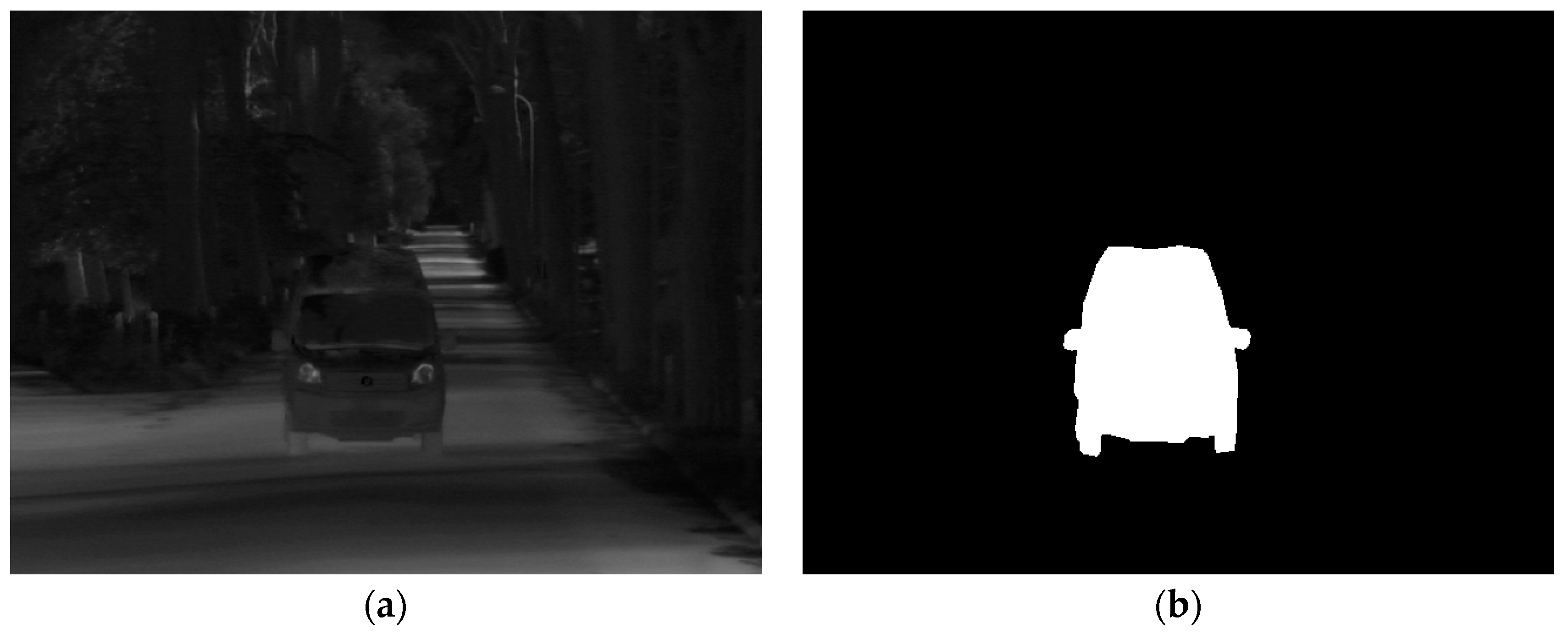
Figure 5.
Example frame of a video sequence containing two moving objects one of which is dim pointed out by the green contour in the zoomed box (a); and corresponding detection map output by the proposed algorithm (b) again the region containing the dim object is pointed out in a zoomed box.
Figure 5.
Example frame of a video sequence containing two moving objects one of which is dim pointed out by the green contour in the zoomed box (a); and corresponding detection map output by the proposed algorithm (b) again the region containing the dim object is pointed out in a zoomed box.
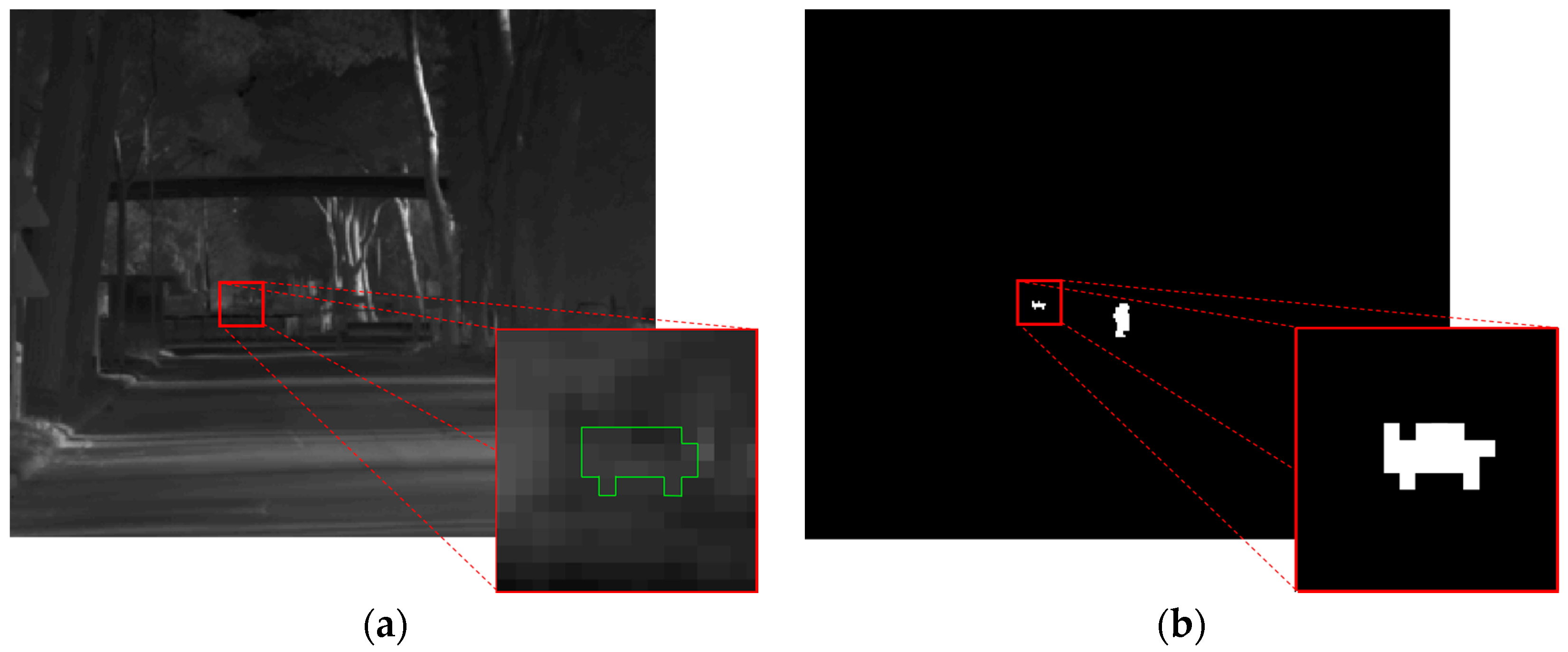
Figure 6.
Example frame of a video sequence containing a slow moving object, contoured in green in the zoomed box (a); and corresponding detection map output by the proposed algorithm (b).
Figure 6.
Example frame of a video sequence containing a slow moving object, contoured in green in the zoomed box (a); and corresponding detection map output by the proposed algorithm (b).
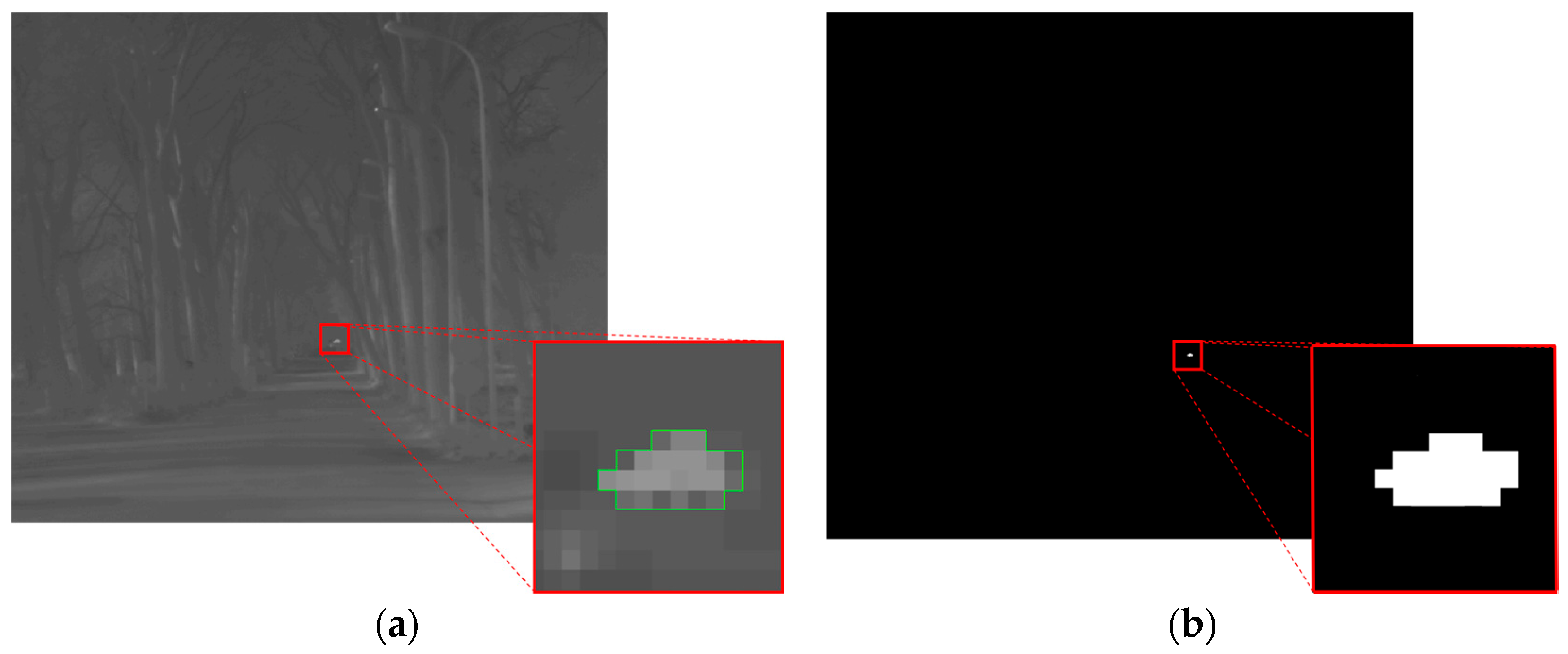
Figure 7.
Plot of: the intensity (after the removal of ), solid blue line; background estimation, solid red line; updating threshold, dashed green lines; and detection threshold, dashed magenta lines over time, for a pixel crossed by a moving object between frames 122 and 784.
Figure 7.
Plot of: the intensity (after the removal of ), solid blue line; background estimation, solid red line; updating threshold, dashed green lines; and detection threshold, dashed magenta lines over time, for a pixel crossed by a moving object between frames 122 and 784.

Figure 8.
Plot on a single frame of all the detections reported in one of the video sequences of the dataset.
Figure 8.
Plot on a single frame of all the detections reported in one of the video sequences of the dataset.


Table 1.
List of the requirements the proposed algorithm should fit.
| Algorithm Requirements |
|---|
| Work in real-time (using low-cost hardware) |
| Low memory allocation |
| Detect both small and large objects |
| Detect dim objects |
| Detect single or multiple objects |
| Detect both fast and slow objects |
| Detect objects that change their velocity/trajectory |
Table 2.
Main specifications of the IR camera used to acquire the video sequences of the dataset.
| IR Camera Specifications | |
|---|---|
| Resolution | 640 × 512 pixels |
| Detector pitch | 15 μm |
| Spectral range | 3.7 ÷ 5.15 μm |
| Temperature range | −20 ÷ 300 °C |
| NETD | 20 mK |
| Focal length | 50 mm |
| F# | f/2 |
| FOV | 11° × 8.8° |
| Frame rate | 25 Hz |
| Data depth | 14 bit |
Table 3.
Performance of the proposed algorithm in the presence of different kinds of moving objects singularly and globally, and comparison with other commonly used DBT algorithms.
Table 3.
Performance of the proposed algorithm in the presence of different kinds of moving objects singularly and globally, and comparison with other commonly used DBT algorithms.
| Proposed Algorithm | FD | GMM | MED | ||
|---|---|---|---|---|---|
| Small objects | 0.973 | 0.724 | 0.971 | 0.974 | |
| 92.9% | 79.2% | 92.5% | 93.3% | ||
| (×10−7) | 2.02 | 2.92 | 2.86 | 3.05 | |
| (ms) | 18.3 | 7.3 | 42.1 | 116.7 | |
| Large objects | 0.997 | 0.963 | 0.992 | 0.995 | |
| 96.1% | 56.3% | 96.4% | 71.2% | ||
| (×10−7) | 2.13 | 3.02 | 2.58 | 8.37 | |
| (ms) | 17.9 | 7.0 | 38.2 | 483.3 | |
| Dim objects | 0.938 | 0.708 | 0.875 | 0.937 | |
| 83.1% | 73.6% | 75.5% | 78.0% | ||
| (×10−7) | 2.81 | 2.90 | 3.15 | 4.61 | |
| (ms) | 16.4 | 6.6 | 39.9 | 206.4 | |
| Fast objects | 0.974 | 0.819 | 0.955 | 0.974 | |
| 93.6% | 90.8% | 93.0% | 94.0% | ||
| (×10−7) | 2.16 | 3.11 | 3.08 | 2.94 | |
| (ms) | 17.3 | 7.1 | 39.2 | 173.8 | |
| Slow objects | 0.922 | 0.628 | 0.918 | 0.898 | |
| 94.2% | 58.4% | 91.5% | 78.6% | ||
| (×10−7) | 2.18 | 2.84 | 3.19 | 11.73 | |
| (ms) | 17.9 | 7.1 | 41.8 | 441.7 | |
| Global result | 0.962 | 0.759 | 0.931 | 0.954 | |
| 91.8% | 70.4% | 89.6% | 87.5% | ||
| (×10−7) | 2.21 | 2.94 | 2.99 | 5.92 | |
| (ms) | 17.5 | 6.89 | 41.4 | 271.7 |
© 2017 by the authors. Licensee MDPI, Basel, Switzerland. This article is an open access article distributed under the terms and conditions of the Creative Commons Attribution (CC BY) license (http://creativecommons.org/licenses/by/4.0/).
Share and Cite
MDPI and ACS Style
Zingoni, A.; Diani, M.; Corsini, G. A Flexible Algorithm for Detecting Challenging Moving Objects in Real-Time within IR Video Sequences. Remote Sens. 2017, 9, 1128. https://doi.org/10.3390/rs9111128
AMA Style
Zingoni A, Diani M, Corsini G. A Flexible Algorithm for Detecting Challenging Moving Objects in Real-Time within IR Video Sequences. Remote Sensing. 2017; 9(11):1128. https://doi.org/10.3390/rs9111128
Chicago/Turabian StyleZingoni, Andrea, Marco Diani, and Giovanni Corsini. 2017. "A Flexible Algorithm for Detecting Challenging Moving Objects in Real-Time within IR Video Sequences" Remote Sensing 9, no. 11: 1128. https://doi.org/10.3390/rs9111128
Note that from the first issue of 2016, this journal uses article numbers instead of page numbers. See further details here.