Urban Sprawl and Adverse Impacts on Agricultural Land: A Case Study on Hyderabad, India
by
 ,
,
Murali Krishna Gumma
1,* ,
,
Irshad Mohammad
1, 
Swamikannu Nedumaran
1,
Anthony Whitbread
1 and
Carl Johan Lagerkvist
2 1
Remote sensing/GIS Lab, Innovation Systems for the Drylands Program (ISD), International Crops Research Institute for the Semi-Arid Tropics (ICRISAT), Patancheru-502324, India
2
Department of Economics, Swedish University of Agricultural Sciences, 75007 Uppsala, Sweden
*
Author to whom correspondence should be addressed.
Remote Sens. 2017, 9(11), 1136; https://doi.org/10.3390/rs9111136
Submission received: 19 September 2017
/
Revised: 2 November 2017
/
Accepted: 3 November 2017
/
Published: 7 November 2017
(This article belongs to the Special Issue Remote Sensing of Urban Agriculture and Land Cover)
Abstract
:Many Indian capitals are rapidly becoming megacities due to industrialization and rural–urban emigration. Land use within city boundaries has changed dynamically, accommodating development while replacing traditional land-use patterns. Using Landsat-8 and IRS-P6 data, this study investigated land-use changes in urban and peri-urban Hyderabad and their influence on land-use and land-cover. Advanced methods, such as spectral matching techniques with ground information were deployed in the analysis. From 2005 to 2016, the wastewater-irrigated area adjacent to the Musi river increased from 15,553 to 20,573 hectares, with concurrent expansion of the city boundaries from 38,863 to 80,111 hectares. Opportunistic shifts in land-use, especially related to wastewater-irrigated agriculture, emerged in response to growing demand for fresh vegetables and urban livestock feed, and to easy access to markets due to the city’s expansion. Validation performed on the land-use maps developed revealed 80–85% accuracy.
1. Introduction
Rapid urbanization and population growth, particularly in developing countries, are expected to increase pressure on agricultural production by expanding into croplands, competing for resources, and leading to loss of biodiversity. By 2050, China, India, and Nigeria alone are expected to add about 900 million urban residents in the megacities of these countries [1]. Managing urban expansion in the future is critical for ensuring agricultural growth and food security, while also providing common amenities such as housing, water, and employment for the growing population. Four of India’s cities (Ahmedabad, Bengaluru, Chennai, and Hyderabad), which currently have 5–10 million inhabitants, are projected to become megacities (population of >10 million) in the coming years, with a total of seven megacities projected in the country by 2030 [2].
Hyderabad is located in Telangana state in southern India and is the sixth largest metropolis in the country. It comprises twelve municipalities, including the Greater Hyderabad Municipal Corporation (GHMC). Hyderabad is located in the Musi sub-basin (11,000 km2), which is part of the Krishna river basin. Rapid development, especially in the information technology (IT) sector, has attracted skilled and unskilled labor from other parts of India, further increasing the city’s population. There is thus an urgent need for city planning to mitigate the impact that rapid development will have on natural resources in the Hyderabad area. In this regard, accurate knowledge of the spatio-temporal pattern of urbanization is very important for policy making, natural resource management, and decision making [3].
Peri-urban agriculture contributes significantly to ecosystem services, serving as a sink for stormwater runoff, a recharge zone for groundwater table, as well as adding to aesthetic beauty and food security [4]. A majority of families in the peri-urban areas of Hyderabad sustain themselves by providing food and animal feed to the city, making these areas important for the local economy [5,6]. A growing population and development in cities increases competition for natural resources (e.g., water and land) and natural diversity [7,8], and shrinks surrounding agricultural areas [9,10]. These changes pose a great challenge to urban developers and the service sector in Hyderabad. Furthermore, urban water demand has grown exponentially in the past two decades and water availability within the city limits of Hyderabad is now inadequate to supply the growing demand, due to encroachment on freshwater lakes to build houses and public offices. Transporting water from nearby rural villages has become a necessity [10]. Agricultural land within the city’s boundaries has been diminishing further with people migrating from rural areas in search of employment and better wages, which is overburdening social and infrastructure services.
Several studies have analyzed sprawl and other land-use/land-cover (LULC) changes in urban areas using satellite imagery. For example, Alqurashi et al. [11] analyzed expansion of urban growth and land-cover changes in five Middle East cities using object-based image analysis, while Cao et al. [12] conducted a study on urban expansion and its impact on land-use patterns using radar graph and gradient-direction methods and landscape matrices. Liu et al. [13] monitored urban expansion in China over the past four decades using satellite imagery while Gumma et al. [9] conducted a study on expansion of urban areas and wastewater-irrigated areas in Hyderabad, India, using Landsat images and supervised classification. Most of these studies used temporal analysis of Landsat imagery. Many studies have demonstrated how to map agricultural areas [14,15,16,17,18,19] using advanced techniques in satellite image analysis; e.g., Parece and Campbell [20] delineated urban impervious surfaces using Landsat imagery and high-resolution aerial photographs in a study conducted in Roanoke, USA. Myint et al. [21] accurately classified urban land cover using high spatial resolution imagery and object-based classification. Zhang et al. [22] assessed impacts of urban expansion on ecosystem services using shared socioeconomic pathways (SSPs) and the land-use scenario dynamics-urban (LUSD-urban) model. However, mapping of urban agricultural areas, including fragmented irrigated areas, has proven to be a challenge due to the diverse range of irrigated plot sizes, crops, and water sources used by farmers [23,24], and the literature has not been able to adequately capture agricultural land-use changes in urban expansion zones. Many studies have used normalized difference vegetation index (NDVI) for monitoring cropland and LULC changes over a set period [25,26,27,28,29,30,31].
The main objective of this study was, therefore, to monitor changes in agriculture and LULC in the areas around Hyderabad, and thereby capture the effects of urban sprawl on land-use. The remote sensing imagery used was Landsat-8 data, IRS-P6 data, and MODIS 250 m 16-bit time series data, combined with ground survey data. Monitoring of agricultural areas is very difficult to capture with single-date imagery [32]. Therefore, the specific methodological contribution of this study relates to the use of unsupervised classification with clusters identified based on bi-spectral plots with high-resolution Google Earth images, spectral profiles, and ground survey data in a combined approach.
The aim in developing an approach based on analyzing high-resolution and coarse-resolution temporal imagery with advanced techniques was to help monitor agriculture and other LULC changes, to understand spatially how urban sprawl influences food security and sustainability in the city of Hyderabad.
2. Study Area
Rapid development, economic growth, and increasing employment opportunities in Hyderabad (301,403 ha) (Figure 1) have attracted people from all over the country, increasing the city’s population to around 8.7 million [33]. The land under agriculture within the city’s boundaries has decreased with infrastructure development, while migration of people from rural areas in search of employment and better wages will only further stress public services. Efforts by the state government of undivided Andhra Pradesh in the 1990s to establish Hyderabad as one of the best IT hubs in the country led to several changes in policies on the development of infrastructure and facilities, as well as in relevant public sectors.
Such development has not been without consequences. For example, the Musi river, a tributary of the Krishna, flows through the city of Hyderabad and has become extremely polluted with discharges from the city. Nevertheless, year-round water supply in the river has encouraged wastewater-irrigated agriculture, within and around the city boundaries, despite the pollution [9,34]. The crops cultivated range from perishable vegetables to cereal crops and animal feed crops, depending on the season, distance from the city, and proximity to markets. In the last two decades, livelihood practices of marginal farmers have changed with urban expansion.
3. Data and Methods
A detailed flowchart of the method followed in this study is presented in Figure 2. Datasets used for the study, at medium and coarse resolution, were obtained from different satellites at different stages of analysis.
3.1. Satellite Images
Three IRS-P6 images obtained from the National Remote Sensing Centre (NRSC, ISRO) were used for monitoring LULC changes in the study area. Two Landsat-8 images (January 2014 and January 2016) and three IRS-P6 images (January 2005, January 2008 and January 2011), which were captured in rabi (postrainy), were extracted from USGS Earth Explorer [35] (see Table 1). Image preprocessing started with image normalization, which involved converting digital numbers (DN) to reflectance values.
MODIS vegetation indices (MOD13Q1 product) were used for class identification and labeling processes. MOD13Q1 data were obtained from USGS LPDAAC [36]. MODIS data were acquired in 12-bit format (0 to 4096 levels) and later stretched to 16-bit (0 to 65,536 levels) and were prepared for the cropping year (June to May) 2004–2005, 2007–2008, 2010–2011, 2013–2014 and 2015–2016 [37,38].
3.2. Image Normalization
The main purpose of normalization is to normalize the multi-date effect [39,40] of IRS-P6 and Landsat-8 images, for better classification. Data from different periods have differing radiometric resolution [41,42] (see Thenkabail et al., 2004, 2003), and hence their respective digital numbers (DNs) carry different levels of information and cannot be directly compared. Therefore, all data were converted to absolute units of radiance (W·m−2·sr−1·μm−1), then to apparent at-satellite reflectance (%), and finally to surface reflectance (%) after atmospheric correction. Details of these conversions are provided below, due to the uniqueness of the sensors involved.
3.2.1. IRS-P6 Data
Since clear Landsat-8 images were not available for the selected dates (Table 1), we decided to use a dataset of similar resolution which was available from IRS-P6. We procured images from the National Remote Sensing Agency (NRSA), India. The IRS-P6 8-bit DN data were converted to spectral radiance using the equation:
where DN is digital number and Gain is saturation radiance for the band.
A reduction in between-scene variability can be achieved through normalization for solar irradiance by converting spectral radiance R, as calculated above, to planetary reflectance or albedo [40]. The combined surface and atmospheric reflectance of the earth is computed with the following formula:
where is the at-satellite exo-atmospheric reflectance, Lλ is the radiance (W·m−2·sr−1·μm−1), d is the earth-to-sun distance in astronomic units at the acquisition date (see [27]), ESUNλ is the mean solar exo-atmospheric irradiance (W·m−2·sr−1·μm−1) or solar flux [43], and is solar zenith angle in degrees (i.e., 90 degrees minus the sun elevation or sun angle when the scene was recorded as given in the image header file).
3.2.2. Landsat-8 Data
The following equation was used to convert DN values to TOA reflectance for OLI data:
where is the TOA planetary reflectance (without correction of solar angle), is the band-specific multiplicative rescaling factor from the metadata, is the band-specific additive rescaling factor from the metadata, and is the quantized and calibrated standard product pixel value (DN).
TOA reflectance with correction for the sun angle is then:
Where, ρλ is the TOA planetary reflectance, ρλ’ is the TOA planetary reflectance without correction of solar angle, and is the local sun elevation angle provided in the metadata (SUN_ELEVATION).
3.3. Ground Survey Datasets
Two ground survey datasets were collected, on 13–26 October 2005, for 130 sampling locations and on 24–29 October 2016, for 132 sampling locations. These locations covered major LULC changes within the study area. The collected data were divided into two datasets, one for class identification and labeling, and the other for validation (Figure 3). Samples were collected based on large continuous homogeneous areas selected as sampling locations. Several parameters were determined at each location, such as cropland including source-wise irrigation, crop type, urban extent including settlements and open land, and other land cover including shrubs, grass, water, fallow, and scrubland. Farmers were interviewed in order to obtain more detailed information on their agricultural fields, which helped to enhance the training data.
The ground survey data were grouped into five categories: water bodies, built-up land, irrigated cropland, rainfed cropland, and “other” LULC.
3.4. Mapping Land-Use/Land-Cover Changes
A comprehensive methodology for mapping cropland areas using IRS-P6 and Landsat-8 data was taken from the literature [27,31,32,44]. Each image was classified using unsupervised ISOCLASS cluster Isodata classification, with 40 classes and 40 maximum iterations and with convergence threshold of 0.99. The main purpose of unsupervised classification is to capture different LULC types within the image across a study area. Simultaneously, we generated mean spectral values for all classes using a signature set option. Class identification and labeling were performed based on spectral properties (bi-spectral plots), ground survey data, and Google Earth high-resolution imagery.
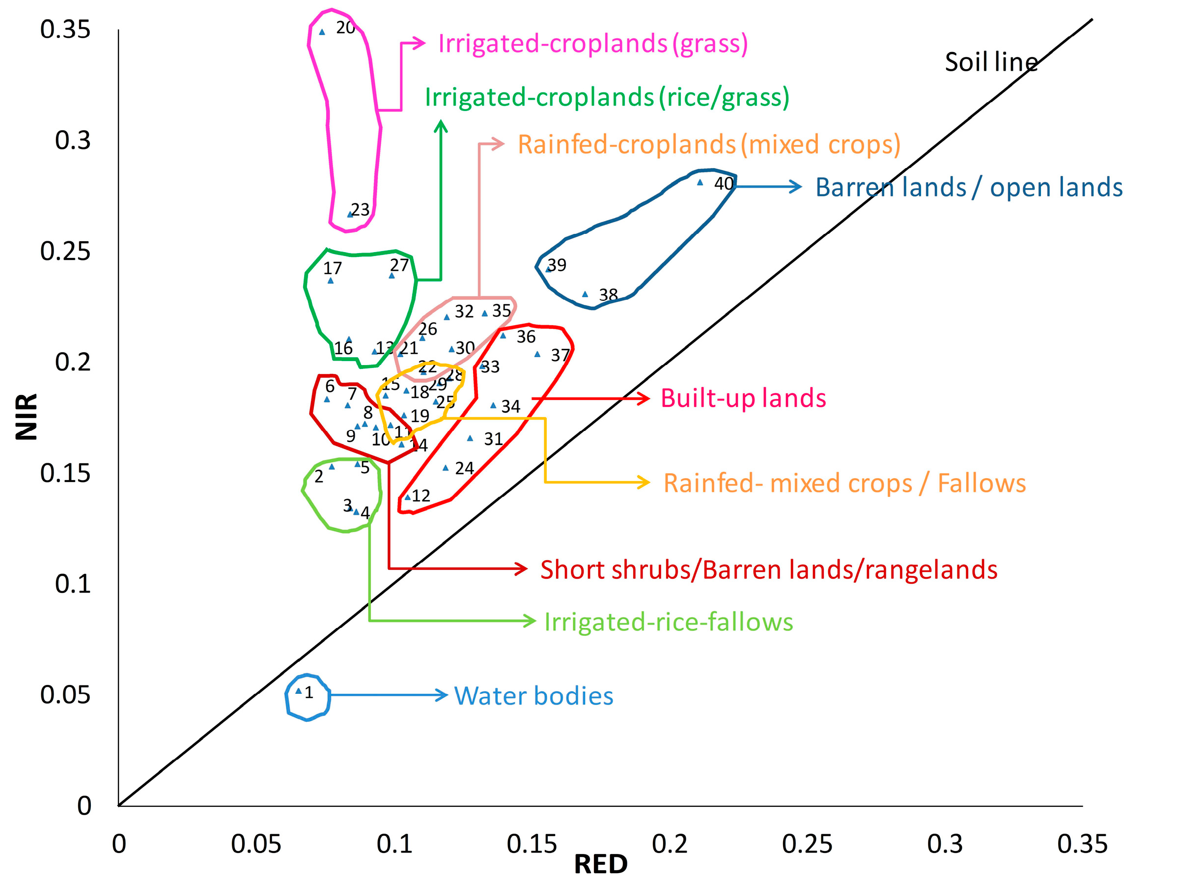
Spectral values of red and NIR bands extracted from unsupervised classification were plotted as shown in Figure 4, with reflectance values of red on the x-axis and reflectance values of NIR on the y-axis) [37,45,46]. In Figure 4, the diagonal line represents the soil line, which differentiated the classes with vegetation. Classes with similar spectral reflectance depict nearby clusters, which may represent the same category (same classes) with a slight variation in reflection. Other classes, like water bodies and shrubland/trees, show large variations in vegetation and can easily be identified and labeled. Classes closer to the soil line and the two-band (red and NIR bands) reflectance values were similar and high; they are classified as built-up areas. More highly vegetated areas, like irrigated cropland, have high reflectance values in NIR and lower reflectance in red.
Spectral profiles were generated from the MODIS time series composite data, with initially 40 unsupervised classes identified based on NDVI profiles at different crop growth stages in the season. Identification and labeling of LULC classes were based on bi-spectral profiles, MODIS NDVI time-series plots, ground survey data, and very-high-resolution images (Google Earth). The specific protocols included grouping class spectra based on class similarities and/or comparing them with ground survey data, rigorous protocols for class identification, and labeling with the use of very high-resolution imagery. After a rigorous classification process, most of the classes were identified, except for some mixed classes.
Validation was performed based on intensive ground survey information through an error matrix, which was generated based on a theoretical description in the literature [47]. The columns of an error matrix contain the ground survey data points, while the rows represent the results of the classified LULC maps [48]. The error matrix is a multidimensional table in which the cells contain changes from one class to another [49]. The 81 points with major LULC and irrigation type observations were used for classification validation. A validation was performed on each LULC map.
3.5. Urban Expansion and Other Land-Use Changes
After class identification and labeling, final LULC maps were validated with ground survey data and used to detect change, based on the 2005 LULC map. The ERDAS modeler was used to quantify changes from 2005 to 2011 and 2005 to 2016, because these three dates were validated using ground survey data and Google Earth high-resolution satellite imagery during the same year. Equation (5) was used to assess changes from 2005 to 2011 and on to 2016. Changes were assessed class-wise, for example, “other” LULC classes and cropland based on the 2005 map were converted to built-up land as:
where is the change detected, LULCi is land-use/land-cover for the ith year and LULCj is land use/land cover for the jth year.
4. Results and Discussion
4.1. Spatio-Temporal Distribution of Land-Use/Land-Cover Changes
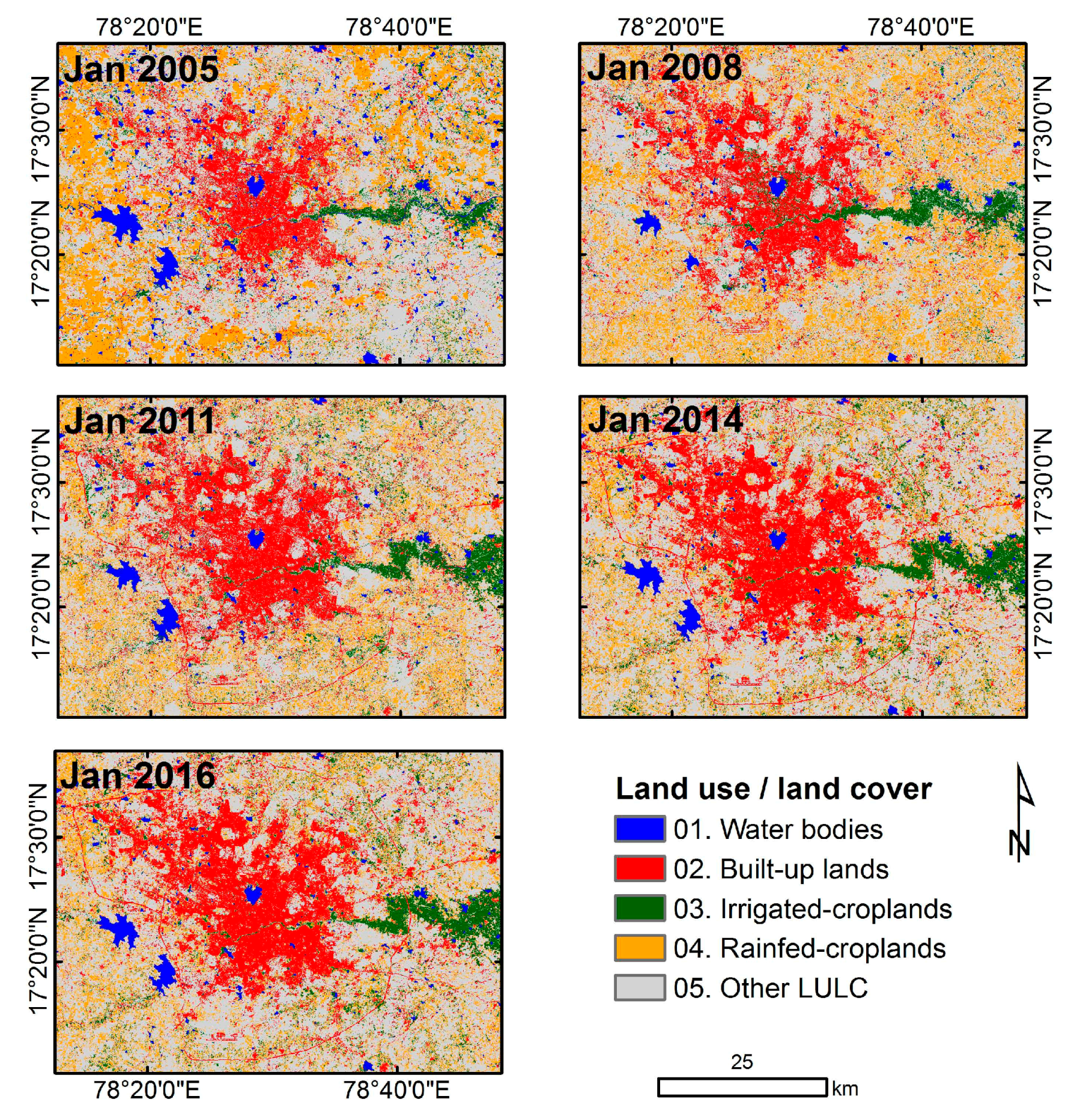
Figure 5 depicts observed changes in the urban sprawl of Hyderabad using IRS-P6 (2005, 2008 and 2011) and Landsat-8 (2014, 2016) imagery. The area covered by built-up land, constituting housing and other buildings, has more than doubled, from 38,863 ha to 80,111 ha, adversely impacting water bodies and rain-fed cropland, the area of which has decreased by half (37,902 ha in 2016 compared to 72,817 ha in 2005) (Table 2). There was a drastic increase in built-up areas in the west and east zones of the city, due to expansion of the IT sector in the former and industrial sector expansion in these zones. Seasonal water bodies appeared to be most exploited for building in the western, central, and southern zones. Similarly, the area under rain-fed cropland, which is now almost halved due to urban expansion, has decreased specifically in the west, east, and north zones. Irrigated cropland area increased from 2005 to 2011, but decreased slightly by 2016 due to low rainfall. An important finding in this study was that wastewater-irrigated agriculture, which is practiced along the banks of the Musi river, has also increased steadily from 2005 to 2016, to support vegetable gardens catering to the growing urban population. Since the formation of the Hyderabad Metropolitan Development Authority (HMDA), with a new master plan, many conservation measures have been established to sustain drinking water sources, such as the lakes Himayath Sagar, Osman Sagar, and Manjeera, and the water supply has been improved. Moreover, a new drinking water pipeline project has been implemented in a phased manner, harnessing water from the Nagarjuna Sagar reservoir [50].
4.2. Validation
Validation was performed based on additional ground survey data (which were not used in classification), and also for individual years. Table 3, Table 4 and Table 5 show the error matrices for the study area during 2005, 2011, and 2016, respectively. Validation was performed by error matrix for whether a known LULC class was correctly classified or not. This process was conducted using 64 ground survey points that referred to one of five classes, as summarized in Table 3. The user accuracy varied from 71% to 100% across the five classes, with an overall accuracy of 81% for 2005, 83% for 2011, and 86% for 2016. Thus, on combining all crop classes into one class, the accuracy of rice mapping was very high (about 95%). The uncertainty in the class results, of about 15%, was due to inter-mixing among the various LULC classes. The accuracy was very high when distinguishing between cropland and non-cropland, while built-up areas and water bodies generally had higher classification accuracy than the “other” LULC and irrigated/rain-fed classes (Table 3, Table 4 and Table 5).
4.3. Urban Expansion and Other Changes
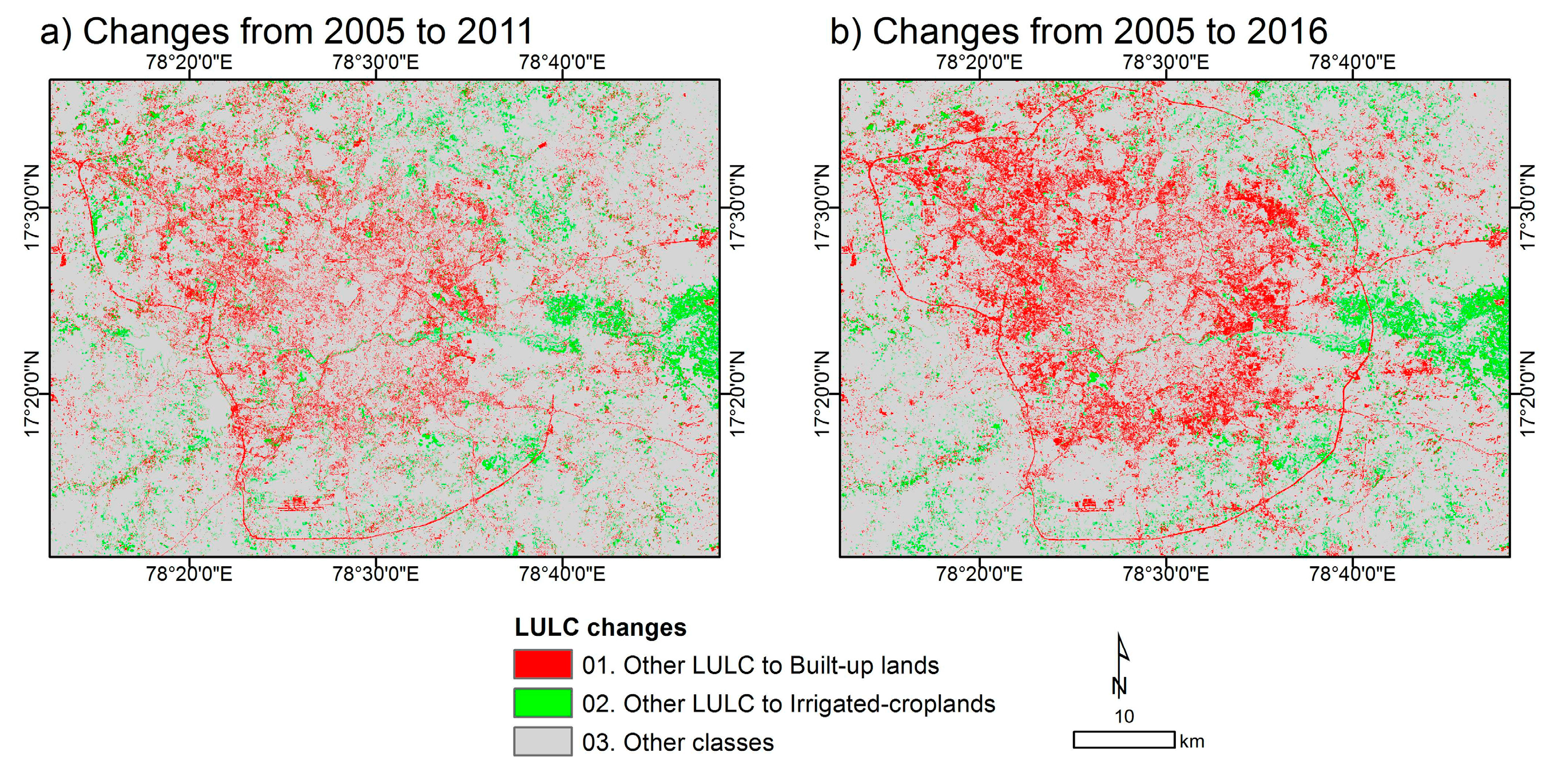
Five-year change detection analysis showed similar changes with respect to irrigated agriculture and other land-use classes (Figure 6). In 2005–2011, the outer ring road (ORR) from the eastern to the southern part of Hyderabad was built [51]. This was also the period when IT companies were starting new projects, the real estate business in the city began to boom, and new pharmaceutical, food, and manufacturing companies were established. This led to immigration of employment seekers from other parts of the country and a high demand for land. Due to this effect, there was transformation from one type of land-use to another, and particularly from cropland to built-up area, with the area of built-up land increasing from 29,684 ha to 41,235 ha during the period (Table 6).
There is a large variety of land uses due to increased urban sprawl in the city of Hyderabad, as shown by satellite image analysis (Table 6, Table 7 and Table 8, Figure 6 and Figure 7). Of the 12,535 ha under water bodies in 2005, around 1900 ha had been converted to agriculture and 1210 ha into built-up land by 2011, and a total of 3016 ha to agriculture and 1345 ha into built-up land by 2016. As a consequence of the loss of water bodies, 2302 ha of irrigated area had been converted to rain-fed agriculture and 1500 ha to built-up land by 2011, and 1709 ha to rain-fed agriculture and 2033 ha to built-up area by 2016. Another important finding was the consistent increase in built-up land from ‘other’ land uses, e.g., rain-fed cropland lost around 7792 ha by 2006 and 9727 ha by 2011. Rain-fed agricultural area decreased consistently from 2005 to 2016, while the clean-water irrigated area did not change during that period.
A significant increase in irrigated area was observed, with water supplied through the use of underground water or wastewater from the Musi river. There has been a drastic increase in wastewater because of urban expansion, which resulted in high use of fresh water. It was also observed that the sprawl is expanding beyond the ORR, which was supposed to regulate the increasingly heavy transport traffic.
4.4. Discusssion on Land-Use/Land-Cover
Mapping built-up land and other LULC using the fusion technique yielded better classification accuracy and helped to decipher LULC patterns, while the temporal LULC maps helped to identify key changes over time and space. In situations of rapid urbanization, planning is necessary to avoid unregulated building, obstruction of drainage lines, and destruction of high-value agricultural lands [52]. Bi-spectral plots have previously been used to map agricultural lands and other LULC for different purposes, such as mapping and classifying irrigated areas, detecting LULC changes, and detecting different land-use categories and cropland categories [28,30,44,53]. Here, we demonstrated its ability to differentiate urban sprawl and other LULC categories. We established LULC classes based on bi-spectral plots, ground survey data, and NDVI temporal profiles, and verified the results using high-resolution maps in Google Earth images for the same years. Alqurashi [11] used object-based image analysis (OBIA) segmentation and classification for mapping LULC in five cities in Saudi Arabia and, depending on the size of patches of LULC, created two levels of image segmentation and classification by adjusting the thresholds in the rules applied. Similarly Cao [12] used an OBIA-based decision tree process to map 13 land-use types, with visual modification employed to improve the classification. Lui et al. [13] used various kinds of automatic classification methods to efficiently map urban areas, and also employed the visual interpretation method combined with professional knowledge to obtain urban boundaries. Even though the accuracy levels are comparable with these different methods, the method developed in the present study is easier and is based on the spectral characteristics of the imagery used. The use of bi-spectral plots is faster and easier when diverse land uses must be distinguished for mapping.
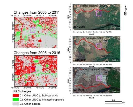
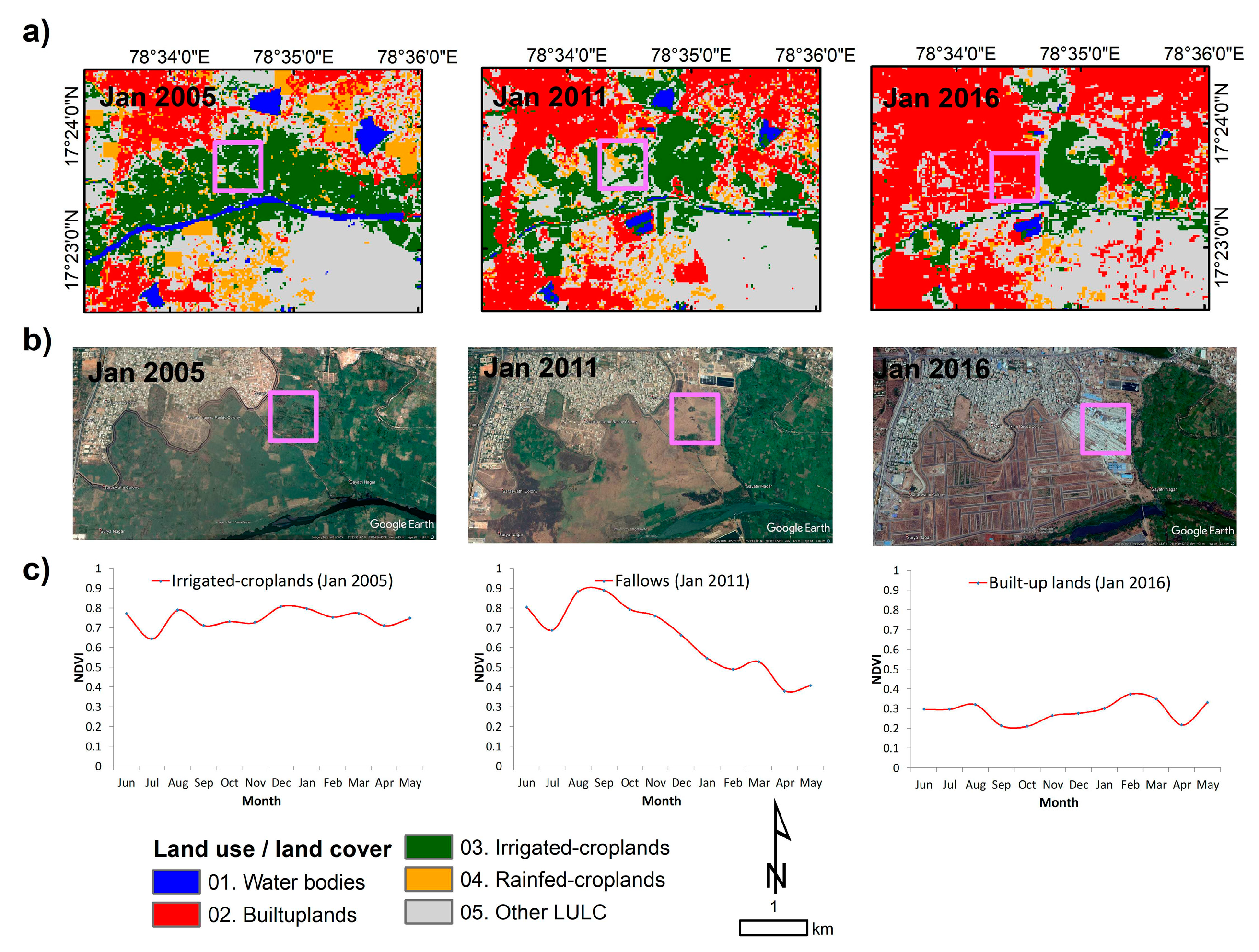
Figure 7 illustrates the spatial and temporal land-use changes for 2005, 2011, and 2016. Using the methodology developed here, the analysis precisely mapped changes in irrigated cropland area to built-up land, and this area was matched with Google Earth high-resolution imagery. The NDVI spectral signatures for different classes (Figure 7c) showed crops continuously under irrigation in 2005, a change to patches of irrigated crops in 2011, and replacement of irrigated cropland with build-up area in 2016.
5. Conclusions
Urban expansion and other LULC changes were analyzed in this study using multi-sensor satellite data such as IRS-P6, Landsat-8, MODIS time series data, and ground survey data. Land-use classes were identified based on bi-spectral plots and ground survey data, and the classes obtained were compared with those in Google Earth high-resolution imagery. The major LULC classes were mapped with error matrix accuracy between 80% and 86%.
The results demonstrate significant strengths in using IRS-P6 23.6 m and MODIS data together with ground survey data in identifying fragmented and minor cropland areas with irrigation sources, such as wastewater irrigation and rain-fed agriculture. However, fragmented mixed cropland areas are better mapped using IRS-P6 data in fusion with coarser-resolution time series data.
The methodology developed in this study is useful in mapping changes in different land uses within a specific geographical area. It is also possible to link information derived from remote sensing to socio-economic variables, which can add a spatial dimension to the picture. In Hyderabad, the most important land cover loss is of water bodies. An increase in wastewater-irrigated agriculture is the most important consequence of this. The vegetable and fruit supply for the city comes from peri-urban areas once under staple food crops (rice, maize, and sorghum), which fed the peri-urban population. The increase in built-up area from 2005 to 2016 has resulted in the loss of 11,760 ha of agricultural land in Hyderabad. The associated reduction in food production is irreversible and this burden has shifted to the surrounding area. The urban sprawl also has impacts on the urban weather profile in terms of expanded heat islands and temperature differences.
Acknowledgments
This work was undertaken as part of the CGIAR Research Programs on Water, Land and Ecosystems (WLE) led by International Water Management Institute (IWMI) and CGIAR Research Programs on Policies, Institutions, and Markets (PIM) led by the International Food Policy Research Institute (IFPRI). Funding support for the study was provided by the Swedish Research Council for Environment, Agricultural Sciences and Spatial Planning (FORMAS) through the Swedish University of Agricultural Sciences (SLU). The authors thank Kristofer Dodge, Consultant, ICRISAT, and Ms Smitha Sitaraman, Science Editor, ICRISAT, for editing this article. The authors are grateful to Padmaja Ravula, Kesav Rao Pyla, Naresh, and NARS partners for supporting the collection of ground data and sub-national statistics.
Author Contributions
The study was proposed by Murali Krishna Gumma, who, together with Swamikannu Nedumaran, Anthony Whitbread and Carl Johan Lagerkvist gave it a direction and contributed to the analysis, results, and discussion. Murali Krishna Gumma and Irshad Ahmed, together with local partners, collected the ground survey data. All the authors drafted their respective contributions.
Conflicts of Interest
The authors declare no conflict of interest.
References
- International Food Policy Research Institute (IFPRI). 2017 Global Food Policy Report; IFPRI: Washington, DC, USA, 2017; Available online: http://www.Ifpri.Org/publication/2017-global-food-policy-report (accessed on 12 October 2017).
- United Nations (UN), Department of Economic and Social Affairs, Population Division (2014). World Urbanization Prospects: The 2014 Revision, Highlights (st/esa/ser.A/352). 2014. Available online: https://esa.Un.Org/unpd/wup/publications/files/wup2014-highlights.Pdf (accessed on 12 October 2017).
- Fan, C.; Myint, S.W.; Rey, S.J.; Li, W. Time series evaluation of landscape dynamics using annual Landsat imagery and spatial statistical modeling: Evidence from the phoenix metropolitan region. Int. J. Appl. Earth Obs. Geoinf. 2017, 58, 12–25. [Google Scholar] [CrossRef]
- Parece, T.E.; Campbell, J.B. Geospatial evaluation for urban agriculture land inventory: Roanoke, virginia USA. Int. J. Appl. Geospat. Res. 2017, 8, 43–63. [Google Scholar] [CrossRef]
- Mougeot, L.J. Urban agriculture: Definition, presence, potentials and risks. In Growing Cities, Growing Food: Urban Agriculture on the Policy Agenda; International Development Research Centre (IDRC): La Habana, Cuba, 2000; pp. 1–2. [Google Scholar]
- Deelstra, T.; Girardet, H. Urban agriculture and sustainable cities. In Growing Cities, Growing Food. Urban Agriculture on the Policy Agenda; Bakker, N., Dubbeling, M., Gündel, S., Sabel-Koshella, U., de Zeeuw, H., Eds.; Zentralstelle für Ernährung und Landwirtschaft (ZEL): Feldafing, Germany, 2000; pp. 43–66. [Google Scholar]
- Scheffers, B.R.; Paszkowski, C.A. The effects of urbanization on north american amphibian species: Identifying new directions for urban conservation. Urban Ecosyst. 2012, 15, 133–147. [Google Scholar] [CrossRef]
- Guderyahn, L.B.; Smithers, A.P.; Mims, M.C. Assessing habitat requirements of pond-breeding amphibians in a highly urbanized landscape: Implications for management. Urban Ecosyst. 2016, 19, 1801–1821. [Google Scholar] [CrossRef]
- Gumma, M.K.; Van Rooijen, D.; Nelson, A.; Thenkabail, P.S.; Aakuraju, R.V.; Amerasinghe, P. Expansion of urban area and wastewater irrigated rice area in Hyderabad, India. Irrig. Drain. Syst. 2011, 25, 135–149. [Google Scholar] [CrossRef]
- Van Rooijen, D.J.; Turral, H.; Wade Biggs, T. Sponge city: Water balance of mega-city water use and wastewater use in Hyderabad, India. Irrig. Drain. 2005, 54. [Google Scholar] [CrossRef]
- Alqurashi, A.; Kumar, L.; Sinha, P. Urban land cover change modelling using time-series satellite images: A case study of urban growth in five cities of Saudi Arabia. Remote Sens. 2016, 8, 838. [Google Scholar] [CrossRef]
- Cao, H.; Liu, J.; Fu, C.; Zhang, W.; Wang, G.; Yang, G.; Luo, L. Urban expansion and its impact on the land use pattern in xishuangbanna since the reform and opening up of China. Remote Sens. 2017, 9, 137. [Google Scholar] [CrossRef]
- Liu, F.; Zhang, Z.; Wang, X. Forms of urban expansion of chinese municipalities and provincial capitals, 1970s–2013. Remote Sens. 2016, 8, 930. [Google Scholar] [CrossRef]
- Ambast, S.K.; Keshari, A.K.; Gosain, A.K. Satellite remote sensing to support management of irrigation systems: Concepts and approaches. Irrig. Drain. 2002, 51, 25–39. [Google Scholar] [CrossRef]
- Bastiaanssen, W.G.M.; Molden, D.J.; Thiruvengadachari, S.; Smit, A.A.M.F.R.; Mutuwatte, L.; Jayasinghe, G. Remote Sensing and Hydrologic Models for Performance Assessment in Sirsa Irrigation Circle, India; International Water Management Institute: Colombo, Sri Lanka, 1999. [Google Scholar]
- Ozdogan, M.; Woodcock, C.E.; Salvucci, G.D. Monitoring changes in summer irrigated crop area in southeastern Turkey using remote sensing. In Proceedings of the 2003 IEEE International Geoscience and Remote Sensing Symposium (IGARSS), Toulouse, France, 21–25 July 2003; pp. 1570–1572. [Google Scholar]
- Sakthivadivel, R.; Thiruvengadachari, S.; Amerasinghe, U.; Bastiaanssen, W.G.M.; Molden, D. Performance Evaluation of the Bhakra Irrigation System, India, Using Remote Sensing and Gis Techniques; International Water Management Institute: Colombo, Sri Lanka, 1999. [Google Scholar]
- Thiruvengadachari, S.; Sakthivadivel, R. Satellite Remote Sensing for Assessment of Irrigation System Performance: A Case Study in India; Research Report 9; International Irrigation Management Institute: Colombo, Sri Lanka, 1997. [Google Scholar]
- Velpuri, N.M.; Thenkabail, P.S.; Gumma, M.K.; Biradar, C.B.; Noojipady, P.; Dheeravath, V.; Yuanjie, L. Influence of resolution in irrigated area mapping and area estimations. Photogramm. Eng. Remote Sens. 2009, 75, 1383–1395. [Google Scholar] [CrossRef]
- Parece, T.E.; Campbell, J.B. Comparing urban impervious surface identification using landsat and high resolution aerial photography. Remote Sens. 2013, 5, 4942–4960. [Google Scholar] [CrossRef]
- Myint, S.W.; Gober, P.; Brazel, A.; Grossman-Clarke, S.; Weng, Q. Per-pixel vs. Object-based classification of urban land cover extraction using high spatial resolution imagery. Remote Sens. Environ. 2011, 115, 1145–1161. [Google Scholar] [CrossRef]
- Zhang, D.; Huang, Q.; He, C.; Wu, J. Impacts of urban expansion on ecosystem services in the Beijing-Tianjin-Hebei urban agglomeration, China: A scenario analysis based on the shared socioeconomic pathways. Resour. Conserv. Recycl. 2017, 125, 115–130. [Google Scholar] [CrossRef]
- Biggs, T.W.; Thenkabail, P.S.; Gumma, M.K.; Scott, C.A.; Parthasaradhi, G.R.; Turral, H.N. Irrigated area mapping in heterogeneous landscapes with MODIS time series, ground truth and census data, krishna basin, India. Int. J. Remote Sens. 2006, 27, 4245–4266. [Google Scholar] [CrossRef]
- Draeger, W.C. Monitoring Irrigated Land Acreage Using Landsat Imagery: An Application Example; Technical Report; U.S. Geological Survey: Ritton, VA, USA, 1976; pp. 1–17.
- Gray, J.; Friedl, M.; Frolking, S.; Ramankutty, N.; Nelson, A.; Gumma, M. Mapping asian cropping intensity with MODIS. IEEE J. Sel. Top. Appl. Earth Obs. Remote Sens. 2014, PP, 1–7. [Google Scholar] [CrossRef]
- Gumma, M.K.; Deevi, K.; Mohammed, I.; Varshney, R.; Gaur, P.; Whitbread, A. Satellite imagery and household survey for tracking chickpea adoption in andhra pradesh, India. Int. J. Remote Sens. 2016, 37, 1955–1972. [Google Scholar] [CrossRef]
- Gumma, M.K.; Gauchan, D.; Nelson, A.; Pandey, S.; Rala, A. Temporal changes in rice-growing area and their impact on livelihood over a decade: A case study of Nepal. Agric. Ecosyst. Environ. 2011, 142, 382–392. [Google Scholar] [CrossRef]
- Gumma, M.K.; Kajisa, K.; Mohammed, I.A.; Whitbread, A.M.; Nelson, A.; Rala, A.; Palanisami, K. Temporal change in land use by irrigation source in Tamil Nadu and management implications. Environ. Monit. Assess. 2015, 187, 1–17. [Google Scholar] [CrossRef] [PubMed]
- Gumma, M.K.; Mohanty, S.; Nelson, A.; Arnel, R.; Mohammed, I.A.; Das, S.R. Remote sensing based change analysis of rice environments in Odisha, India. J. Environ. Manag. 2015, 148, 31–41. [Google Scholar] [CrossRef] [PubMed]
- Gumma, M.K.; Thenkabail, P.S.; Maunahan, A.; Islam, S.; Nelson, A. Mapping seasonal rice cropland extent and area in the high cropping intensity environment of Bangladesh using MODIS 500 m data for the year 2010. ISPRS J. Photogramm. Remote Sens. 2014, 91, 98–113. [Google Scholar] [CrossRef]
- Gumma, M.K.; Thenkabail, P.S.; Muralikrishna, I.V.; Velpuri, M.N.; Gangadhararao, P.T.; Dheeravath, V.; Biradar, C.M.; Acharya Nalan, S.; Gaur, A. Changes in agricultural cropland areas between a water-surplus year and a water-deficit year impacting food security, determined using MODIS 250 m time-series data and spectral matching techniques, in the krishna river basin (India). Int. J. Remote Sens. 2011, 32, 3495–3520. [Google Scholar] [CrossRef]
- Gumma, M.K.; Thenkabail, P.S.; Hideto, F.; Nelson, A.; Dheeravath, V.; Busia, D.; Rala, A. Mapping irrigated areas of Ghana using fusion of 30 m and 250 m resolution remote-sensing data. Remote Sens. 2011, 3, 816–835. [Google Scholar] [CrossRef]
- World Population Review (WPR). Hyderabad Population 2017, World Population Review. 2017. Available online: http://worldpopulationreview.Com/world-cities/hyderabad-population/ (accessed on 21 July 2017).
- Van Rooijen, D.J.; Biggs, T.W.; Smout, I.; Drechsel, P. Urban growth, wastewater production and use in irrigated agriculture: A comparative study of accra, Addis Ababa and Hyderabad. Irrig. Drain. Syst. 2010, 24, 53–64. [Google Scholar] [CrossRef] [Green Version]
- United States Geological Survey (USGS) Earth Explores. Available online: https://earthexplorer.Usgs.Gov/ (accessed on 10 August 2017).
- Land Processes Distributed Active Archive Center (LPDAAC). LP DAAC:: NASA Land Data Products and Services—USGS. Available online: https://e4ftl01.Cr.Usgs.Gov/molt/mod13q1.006/ (accessed on 10 August 2017).
- Thenkabail, P.S.; Schull, M.; Turral, H. Ganges and indus river basin land use/land cover (LULC) and irrigated area mapping using continuous streams of MODIS data. Remote Sens. Environ. 2005, 95, 317–341. [Google Scholar] [CrossRef]
- Gumma, M.K.; Thenkabail, P.S.; Teluguntla, P.; Rao, M.N.; Mohammed, I.A.; Whitbread, A.M. Mapping rice-fallow cropland areas for short-season grain legumes intensification in South Asia using MODIS 250 m time-series data. Int. J. Digit. Earth 2016, 9, 981–1003. [Google Scholar] [CrossRef] [Green Version]
- Markham, B.L.; Barker, J.L. Landsat MSS and TM Post-Calibration Dynamic Ranges, Exoatmospheric Reflectances and At-Satellite Temperatures; Landsat Technical Notes; Earth Observation Satellite Company: Lanham, MD, USA, 1986; Volume 1. [Google Scholar]
- Gumma, M.K.; Pyla, K.; Thenkabail, P.; Reddi, V.; Naresh, G.; Mohammed, I.; Rafi, I. Crop dominance mapping with irs-p6 and MODIS 250-m time series data. Agriculture 2014, 4, 113–131. [Google Scholar] [CrossRef] [Green Version]
- Thenkabail, P.S.; Enclona, E.A.; Ashton, M.S.; Legg, C.; De Dieu, M.J. Hyperion, IKONOS, ALI, and ETM+ sensors in the study of african rainforests. Remote Sens. Environ. 2004, 90, 23–43. [Google Scholar] [CrossRef]
- Thenkabail, P. Biophysical and yield information for precision farming from near-real-time and historical Landsat tm images. Int. J. Remote Sens. 2003, 24, 2879–2904. [Google Scholar] [CrossRef]
- Neckel, H.; Labs, D. The solar radiation between 3300 and 12500 Å. Sol. Phys. 1984, 90, 205–258. [Google Scholar] [CrossRef]
- Gumma, M.K.; Nelson, A.; Thenkabail, P.S.; Singh, A.N. Mapping rice areas of South Asia using MODIS multitemporal data. J. Appl. Remote Sens. 2011, 5, 053547. [Google Scholar] [CrossRef]
- Gumma, M.K. Methods and Approaches for Irrigated Area Mapping at Various Spatial Resolutions Using Avhrr, MODIS and Landsat ETM+ Data for the Krishna River Basin, India. Ph.D. Thesis, Jawaharlal Nehru Technological University Hyderabad, Hyderabad, Telangana, India, 2008. Available online: http://publications.iwmi.org/pdf/H042567.pdf (accessed on 5 Sepetmber 2017).
- Krishna, G.M.; Prasad, T.S.; Bubacar, B. Delineating shallow ground water irrigated areas in the atankwidi watershed (northern Ghana, Burkina faso) using quickbird 0.61–2.44 meter data. Afr. J. Environ. Sci. Technol. 2010, 4, 455–464. [Google Scholar]
- Jensen, J.R. Iintroductory Digital Image Processing: A Remote Sensing Perspective, 3rd ed.; Prentice Hall: Upper Saddle River, NJ, USA, 2004; p. 544. [Google Scholar]
- Congalton, R.G. A review of assessing the accuracy of classifications of remotely sensed data. Remote Sens. Environ. 1991, 37, 35–46. [Google Scholar] [CrossRef]
- Congalton, R.G.; Green, K. Assessing the Accuracy of Remotely Sensed Data: Principles and Practices; Lewis: New York, NY, USA, 1999. [Google Scholar]
- Hyderabad Metropolitan Water Supply and Sewerage Board (HMWSSB). Available online: Http://www.Hyderabadwater.Gov.In/en/index.Php/projects_view?Projectid=946 (accessed on 10 August 2017).
- Hyderabad Metropolitan Development Authority (HMDA). Outer Ring Road. Available online: Https://www.Hmda.Gov.In/orr.Aspx (accessed on 10 August 2017).
- Depietri, Y.; Renaud, F.G.; Kallis, G. Heat waves and floods in urban areas: A policy-oriented review of ecosystem services. Sustain. Sci. 2012, 7, 95–107. [Google Scholar] [CrossRef]
- Thenkabail, P.; GangadharaRao, P.; Biggs, T.; Gumma, M.; Turral, H. Spectral matching techniques to determine historical land-use/land-cover (lulc) and irrigated areas using time-series 0.1-degree avhrr pathfinder datasets. Photogramm. Eng. Remote Sens. 2007, 73, 1029–1040. [Google Scholar]
Figure 1.
Maps of the study area showing different features: (a) Greater Hyderabad Municipal Corporation (GHMC); (b) location of study area and (c) different zones in GHMC.
Figure 1.
Maps of the study area showing different features: (a) Greater Hyderabad Municipal Corporation (GHMC); (b) location of study area and (c) different zones in GHMC.
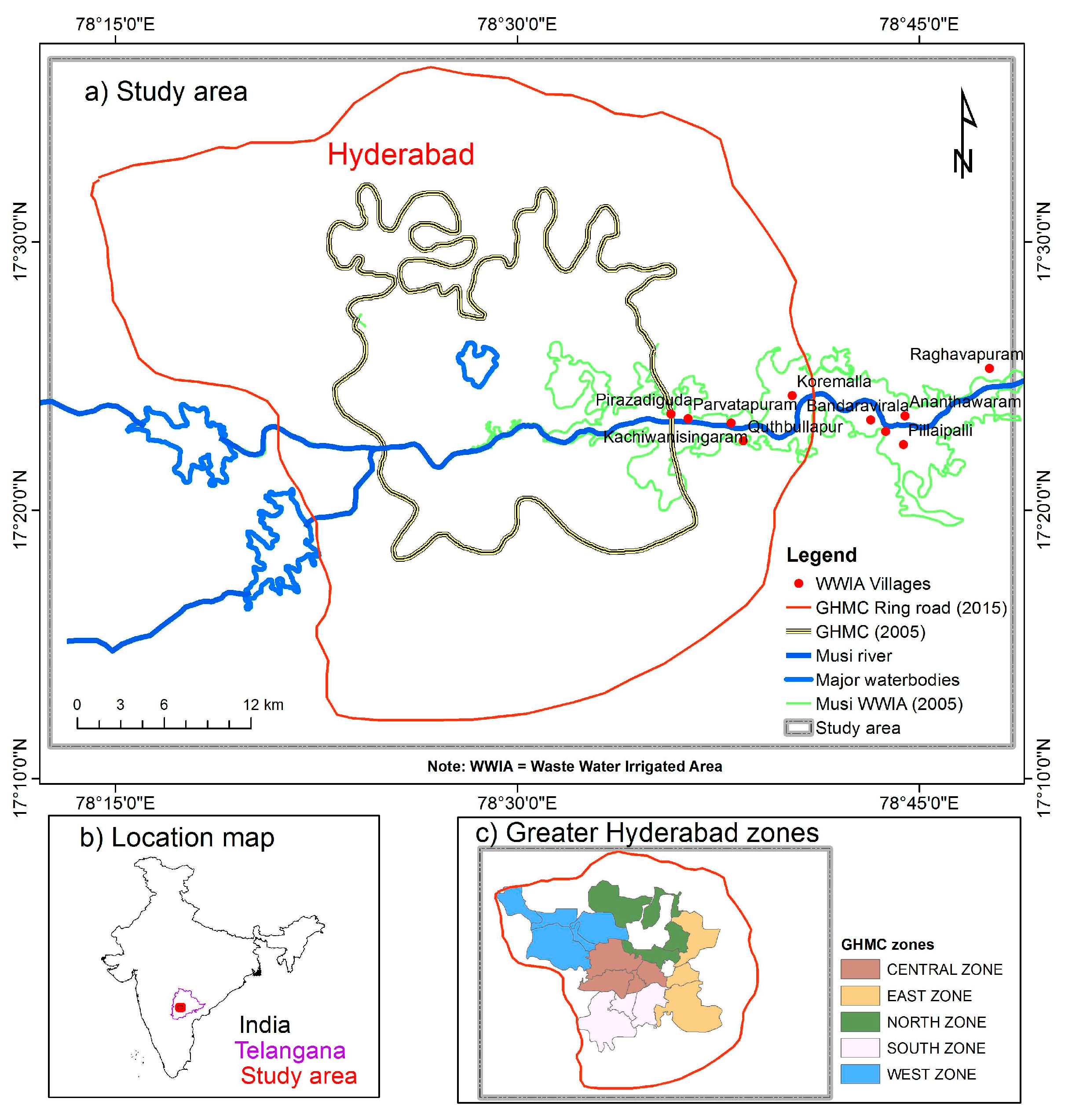
Figure 2.
An overviews of the methodology used to map urban areas and other land-use/land-cover (LULC) changes using Landsat-8 data.
Figure 2.
An overviews of the methodology used to map urban areas and other land-use/land-cover (LULC) changes using Landsat-8 data.
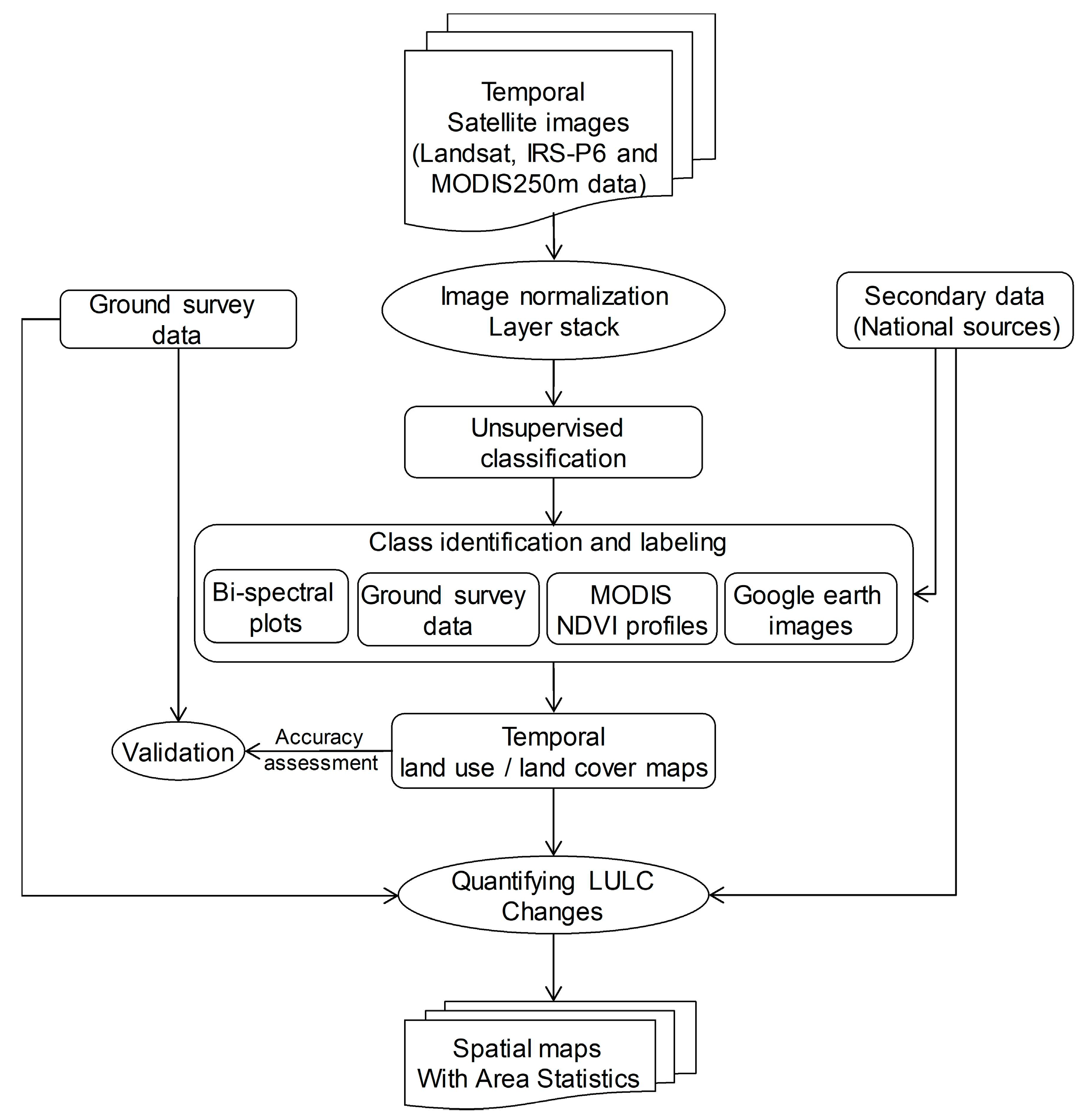
Figure 3.
Spatial distribution of ground survey data in the study area in different periods.
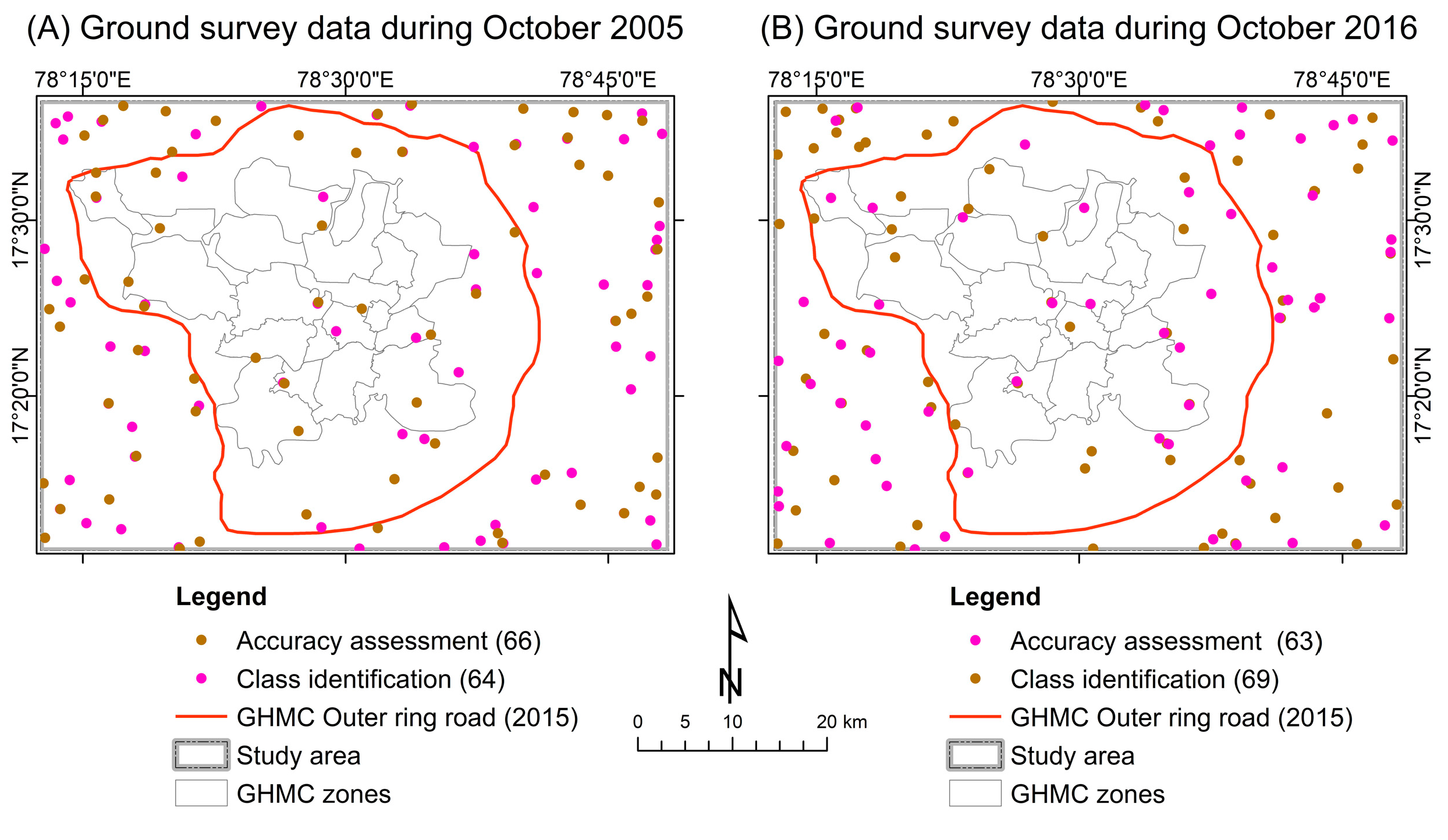
Figure 4.
Single-date bi-spectral plot of unsupervised classes plotted by mean class reflectance in the red and NIR bands.
Figure 4.
Single-date bi-spectral plot of unsupervised classes plotted by mean class reflectance in the red and NIR bands.

Figure 5.
The five land-use/land-cover (LULC) classes developed, based on Landsat-8, IRS-P6, and MODIS time series data, for the years 2005, 2008, 2011, 2014, and 2016.
Figure 5.
The five land-use/land-cover (LULC) classes developed, based on Landsat-8, IRS-P6, and MODIS time series data, for the years 2005, 2008, 2011, 2014, and 2016.

Figure 6.
Land-use/land-cover (LULC) changes between 2005 and 2011 and between 2005 and 2016, based on Landsat-8, IRS-P6, and MODIS time series data.
Figure 6.
Land-use/land-cover (LULC) changes between 2005 and 2011 and between 2005 and 2016, based on Landsat-8, IRS-P6, and MODIS time series data.

Figure 7.
Example of temporal changes in 2005, 2011, and 2016. (a) The land-use/land-cover (LULC) classes; (b) true-color Google Earth imagery for the same LULC classes map; and (c) MODIS-derived NDVI signatures for 2005, 2011 and 2016.
Figure 7.
Example of temporal changes in 2005, 2011, and 2016. (a) The land-use/land-cover (LULC) classes; (b) true-color Google Earth imagery for the same LULC classes map; and (c) MODIS-derived NDVI signatures for 2005, 2011 and 2016.

Table 1.
Characteristics of satellite data used in this study.
| Sensor/Image Acquisition Date | Spatial (m) | No. of Bands | Band Range (µm) | Irradiance (W·m−2·sr−1·mm−1) | Potential Application |
|---|---|---|---|---|---|
| IRS-P6 January 2005 January 2008 January 2011 | 23.6 | 2 | 0.52–0.59 | 1857.7 | Water bodies and also capable of differentiating soil and rock surfaces from vegetation |
| 3 | 0.62–0.68 | 1556.4 | Sensitive to water turbidity differences | ||
| 4 | 0.77–0.86 | 1082.4 | Sensitive to strong chlorophyll absorption region and strong reflectance region for most soils. | ||
| 5 | 1.55–1.70 | 239.84 | Operates in the best spectral region to distinguish vegetation varieties and conditions | ||
| Landsat-8 January 2014, January 2016 | 30 | 1 | 0.43–0.45 | 555 | Water bodies and also capable of differentiating soil and rock surfaces from vegetation |
| 2 | 0.45–0.51 | 581 | |||
| 3 | 0.53–0.59 | 544 | Sensitive to water turbidity differences | ||
| 4 | 0.64–0.67 | 462 | Sensitive to strong chlorophyll absorption region and strong reflectance region for most soils. | ||
| 5 | 0.85–0.88 | 281 | Especially important for the ecology because healthy plants reflect it | ||
| 6 | 1.57–1.65 | 71.3 | Particularly useful for telling wet earth from dry earth, and for geology: rocks and soils that look similar in other bands often have strong contrasts in SWIR. | ||
| 7 | 2.11–2.09 | 24.3 | |||
| MODIS (2005–2016) | 250 | 1 | 0.62–0.67 | 1528.2 | Absolute Land Cover Transformation, Vegetation Chlorophyll |
| 2 | 0.84–0.88 | 974.3 | Cloud Amount, Vegetation Land Cover Transformation |
Table 2.
Selected land-use/land-cover (LULC) data for the years 2005, 2008, 2011, 2014 and 2016.
| LULC | Area (Ha) | ||||
|---|---|---|---|---|---|
| 2005 | 2008 | 2011 | 2014 | 2016 | |
| 01. Water bodies | 12,535 | 3584 | 5417 | 5694 | 2283 |
| 02. Built-up land | 38,863 | 62,000 | 68,560 | 74,131 | 80,111 |
| 03. Irrigated cropland | 15,553 | 14,589 | 19,966 | 19,510 | 19,678 |
| 04. Rainfed cropland | 72,817 | 69,601 | 53,361 | 46,815 | 37,902 |
| 05. Other LULC | 161,635 | 151,562 | 154,288 | 155,445 | 161,583 |
Table 3.
Validation of land-use/land-cover (LULC) classes in 2005 based on ground survey data.
| Classified Data | Reference Data (Ground Survey Data) | |||||||||
|---|---|---|---|---|---|---|---|---|---|---|
| 01. Water Bodies | 02. Built-Up Land | 03. Irrigated Cropland | 04. Rainfed Cropland | 05. Other LULC | Row Total | Number Correct | Producer Accuracy | User Accuracy | Kappa | |
| 01. Water bodies | 11 | 0 | 0 | 0 | 0 | 11 | 11 | 100% | 100% | 100% |
| 02. Built-up land | 0 | 6 | 0 | 0 | 0 | 6 | 6 | 75% | 100% | 100% |
| 03. Irrigated cropland | 0 | 0 | 3 | 0 | 1 | 4 | 3 | 50% | 75% | 72% |
| 04. Rainfed cropland | 0 | 0 | 1 | 10 | 1 | 12 | 10 | 67% | 83% | 78% |
| 05. Other LULC | 0 | 2 | 2 | 5 | 22 | 31 | 22 | 92% | 71% | 54% |
| Column Total | 11 | 8 | 6 | 15 | 24 | 64 | 52 | |||
| Overall classification accuracy = 81.25% | Overall kappa statistic = 0.7422 | |||||||||
Table 4.
Validation of land-use/land-cover (LULC) classes in 2011, based on ground survey data.
| Classified Data | Reference Data (Ground Survey Data) | |||||||||
|---|---|---|---|---|---|---|---|---|---|---|
| 01. Water Bodies | 02. Built-up Land | 03. Irrigated Cropland | 04. Rainfed Cropland | 05. Other LULC | Row Total | Number Correct | Producer Accuracy | User Accuracy | Kappa | |
| 01. Water bodies | 9 | 0 | 1 | 0 | 0 | 10 | 9 | 100% | 90% | 88% |
| 02. Built-up land | 0 | 12 | 0 | 0 | 0 | 12 | 12 | 100% | 100% | 100% |
| 03. Irrigated cropland | 0 | 0 | 5 | 1 | 1 | 7 | 5 | 71% | 71% | 68% |
| 04. Rainfed cropland | 0 | 0 | 0 | 4 | 2 | 6 | 4 | 44% | 67% | 61% |
| 05. Other LULC | 0 | 0 | 1 | 4 | 20 | 25 | 20 | 87% | 80% | 68% |
| Column Total | 9 | 12 | 7 | 9 | 23 | 60 | 50 | |||
| Overall classification accuracy = 83.33% | Overall kappa statistic = 0.7768 | |||||||||
Table 5.
Validation of land-use/land-cover (LULC) classes in 2016, based on ground survey data.
| Classified Data | Reference Data (Ground Survey Data) | |||||||||
|---|---|---|---|---|---|---|---|---|---|---|
| 01. Water Bodies | 02. Built-Up Land | 03. Irrigated Cropland | 04. Rainfed Cropland | 05. Other LULC | Row Total | Number Correct | Producer Accuracy | User Accuracy | Kappa | |
| 01. Water bodies | 8 | 0 | 0 | 0 | 0 | 8 | 8 | 80% | 100% | 100% |
| 02. Built-up land | 0 | 12 | 0 | 0 | 1 | 13 | 12 | 100% | 92% | 91% |
| 03. Irrigated cropland | 1 | 0 | 7 | 0 | 0 | 8 | 7 | 70% | 88% | 85% |
| 04. Rainfed cropland | 0 | 0 | 0 | 1 | 0 | 1 | 1 | 20% | 100% | 100% |
| 05. Other LULC | 1 | 0 | 3 | 4 | 31 | 39 | 31 | 97% | 79% | 62% |
| Column Total | 10 | 12 | 10 | 5 | 32 | 69 | 59 | |||
| Overall classification accuracy = 85.51% | Overall kappa statistic = 0.7838 | |||||||||
Table 6.
Matrix of Land-use/land-cover (LULC) changes from 2005 to 2011.
| Land-Use/Land-Cover (2011) | Land-Use/Land-Cover, Ha (2005) | ||||
|---|---|---|---|---|---|
| 01. Water Bodies | 02. Built-Up Land | 03. Irrigated Cropland | 04. Rain-Fed Cropland | 05. Other LULC | |
| 01. Water bodies | 5011 | 0 | 126 | 94 | 186 |
| 02. Built-up land | 1212 | 38,863 | 1500 | 7792 | 19,180 |
| 03. Irrigated cropland | 1790 | 0 | 4265 | 5620 | 8278 |
| 04. Rainfed cropland | 1114 | 0 | 2302 | 17292 | 32,604 |
| 05. Other LULC | 3406 | 0 | 7358 | 42,010 | 101,367 |
Table 7.
Matrix of Land-use/land-cover (LULC) changes from 2005 to 2016.
| Land-Use/Land-Cover (2016) | Land-Use/Land-Cover, Ha (2005) | ||||
|---|---|---|---|---|---|
| 01. Water Bodies | 02. Built-Up Land | 03. Irrigated Cropland | 04. Rain-Fed Cropland | 05. Other LULC | |
| 01. Water bodies | 2012 | 0 | 71 | 60 | 140 |
| 02. Built-up land | 1345 | 38,863 | 2033 | 9727 | 28,130 |
| 03. Irrigated cropland | 1890 | 0 | 4361 | 5339 | 8069 |
| 04. Rainfed cropland | 1126 | 0 | 1709 | 11,874 | 23,155 |
| 05. Other LULC | 6161 | 0 | 7376 | 45,801 | 102,114 |
Table 8.
Changes in the area (ha) of “other” land-use/land-cover (LULC) to built-up land and irrigated cropland between 2005 and 2011 and between 2005 and 2016.
Table 8.
Changes in the area (ha) of “other” land-use/land-cover (LULC) to built-up land and irrigated cropland between 2005 and 2011 and between 2005 and 2016.
| LULC Changes | Area (Ha) | |
|---|---|---|
| 2005 to 2011 | 2005 to 2016 | |
| 01. Other LULC to built-up land | 29,684 | 41,235 |
| 02. Other LULC to irrigated cropland | 15,688 | 15,297 |
| 03. Other classes | 256,221 | 245,062 |
© 2017 by the authors. Licensee MDPI, Basel, Switzerland. This article is an open access article distributed under the terms and conditions of the Creative Commons Attribution (CC BY) license (http://creativecommons.org/licenses/by/4.0/).
Share and Cite
MDPI and ACS Style
Gumma, M.K.; Mohammad, I.; Nedumaran, S.; Whitbread, A.; Lagerkvist, C.J. Urban Sprawl and Adverse Impacts on Agricultural Land: A Case Study on Hyderabad, India. Remote Sens. 2017, 9, 1136. https://doi.org/10.3390/rs9111136
AMA Style
Gumma MK, Mohammad I, Nedumaran S, Whitbread A, Lagerkvist CJ. Urban Sprawl and Adverse Impacts on Agricultural Land: A Case Study on Hyderabad, India. Remote Sensing. 2017; 9(11):1136. https://doi.org/10.3390/rs9111136
Chicago/Turabian StyleGumma, Murali Krishna, Irshad Mohammad, Swamikannu Nedumaran, Anthony Whitbread, and Carl Johan Lagerkvist. 2017. "Urban Sprawl and Adverse Impacts on Agricultural Land: A Case Study on Hyderabad, India" Remote Sensing 9, no. 11: 1136. https://doi.org/10.3390/rs9111136
Note that from the first issue of 2016, this journal uses article numbers instead of page numbers. See further details here.