1. Introduction
Impervious surfaces are mainly artificial structures that do not allow water to infiltrate into the ground surface. They include rooftops, driveways, sidewalks, parking lots, and roads, and have been recognized as a key indicator of urban environments [
1]. Apart from being a major component of urban land cover [
2,
3], impervious surfaces also play a key role in urban climate [
4], urban heat land effect [
5], and regional ecological and hydrological systems [
6,
7]. With the rapid growth of urban populations, impervious surfaces will undoubtedly continue to grow around the world, especially in developing countries [
8,
9]. Therefore, long-term and detailed information on the spatial-temporal change of impervious surfaces is significant for quantifying the rate of rapid urbanization and predicting its environmental effects.
In the past decades, impervious surfaces have been successfully monitored with remotely-sensed imagery over a wide range of spatial scales and using a variety of data sources [
8]. Multispectral imagery has been widely used for the extraction of impervious surfaces, such as Moderate resolution imaging spectroradiometer (MODIS) data, Landsat Thematic Mapper/Enhanced Thematic Mapper Plus/Operational Land Imager (TM/ETM+/OLI) data, and Advanced Spaceborne Thermal Emission and Reflection Radiometer (ASTER) data. The Defense Meteorological Satellite Program’s Operational Linescan System (DMSP-OLS) images have also been used to map impervious surfaces based on observed city night lights. Moreover, light detection and ranging (LiDAR) and synthetic aperture radar (SAR) images have been increasingly employed to detect urban and impervious areas, because of the excellent performance in vertical structure measurements [
10,
11,
12]. Among all of the remotely sensed imagery used for impervious surfaces mapping, Landsat sensor data are perhaps the most popular because of the unparalleled temporal span together with its relatively fine spatial resolution and spectral coverage.
Numerous methods have been developed for mapping impervious surfaces, from mono-temporal Landsat satellite data, such as spectral mixture analysis [
13,
14,
15], index methods [
16,
17,
18], decision tree models [
19,
20,
21,
22,
23,
24], regression models [
25,
26], and machine learning methods [
27,
28]. Moreover, change detection techniques have also been applied with multi-temporal images to analyze the spatial-temporal pattern of urban expansion. For example, Gao et al. [
29] utilized Landsat data to map impervious surface expansion in Yangtze River Delta, China, for nine periods from 1973 to 2006. Schneider [
9] employed Landsat TM and ETM+ data to study the urban expansion of 143 Chinese cities covering seven years from 1978 to 2010. Sexton et al. [
30] monitored the long-term land cover change in the Piedmont Plateau via multi-temporal classification across the Landsat 5 record.
With the Landsat archive opened for free access since 2008, it is possible to acquire Landsat satellite data from the past 40 years. Due to the long record of continuous measurement provided by the Landsat archive, the mapping of impervious surfaces at a high temporal resolution (e.g., annual) became possible, and has been considered as a promising approach to accurately analyze the temporal pattern of impervious surfaces. For example, Sexton et al. [
31] used the Landsat records to monitor the urban growth in the Washington, D.C.–Baltimore, MD metropolitan region from 1984 to 2010 at an annual frequency. Zhang et al. [
32] proposed a temporal filtering method to improve impervious surfaces classification for each year from dense Landsat time-series datasets in the Pearl River Delta over 23 years. Song et al. [
33] proposed an approach for detecting and characterizing land use/cover change as continuous fields by utilizing the temporal smoothing technique to remove classification noise. Li et al. [
34] proposed a temporal consistency check method to improve the accuracy of urban areas mapping of Beijing from 1984 to 2013. Li et al. [
35] fused Google Earth images and Landsat images to estimate the fine spatial and temporal land cover change pattern.
Compared with the approaches using a single image or a few multi-temporal images for impervious surfaces mapping, an important advantage of using long time-series data is that the land cover label errors caused by the image classification procedure can be eliminated to some extent with the application of a temporal consistency (TC) model [
3,
32,
34]. A TC model is generally considered to be a post-classification processing method that aims to correct the initial misclassified land cover labels of remotely sensed images by using the temporal contextual land cover information. Previous studies have shown that using a TC model can produce more accurate classification results.
However, in practice, most existing TC models are only based on the resultant serial land cover maps produced by the image classification method used. This means that only class labels are employed in these TC models, while the uncertainty in the classification process is ignored. It is noted that remotely sensed data unavoidably contains uncertainty, which is caused by the interference of environment and the limitations of data acquisition and processing devices [
36]. As a result, the uncertainty in remote sensing data needs to be estimated [
37]. Therefore, for most remote sensing image classification methods, besides the resultant land cover map, the classification with uncertainty can also be used to provide prior information for land cover mapping [
38]. Previous studies have shown that the incorporation of uncertainty in the classification of remote sensing images can produce a considerable improvement in the accuracy of the classification [
39]. Since the class label with uncertainty information is more reliable, it is expected that the performance of TC models can be enhanced by the incorporation of the uncertainty information of the land cover class labels into the analysis.
In this paper, an uncertainty-based spatial-temporal consistency (USTC) model was proposed to improve the accuracy of long time series impervious surface classifications. The goal of this paper is twofold. First, we aim to establish a USTC model, which was used to account for the spatial-temporal consistency of the underlying land cover process. The second goal is to apply the proposed USTC model to the 30 years Landsat time-series datasets for Wuhan city in order to validate the proposed USTC model, and quantify the expansion of the city’s impervious surfaces from 1987 to 2016.
2. Materials and Methods
2.1. Study Area and Data Used
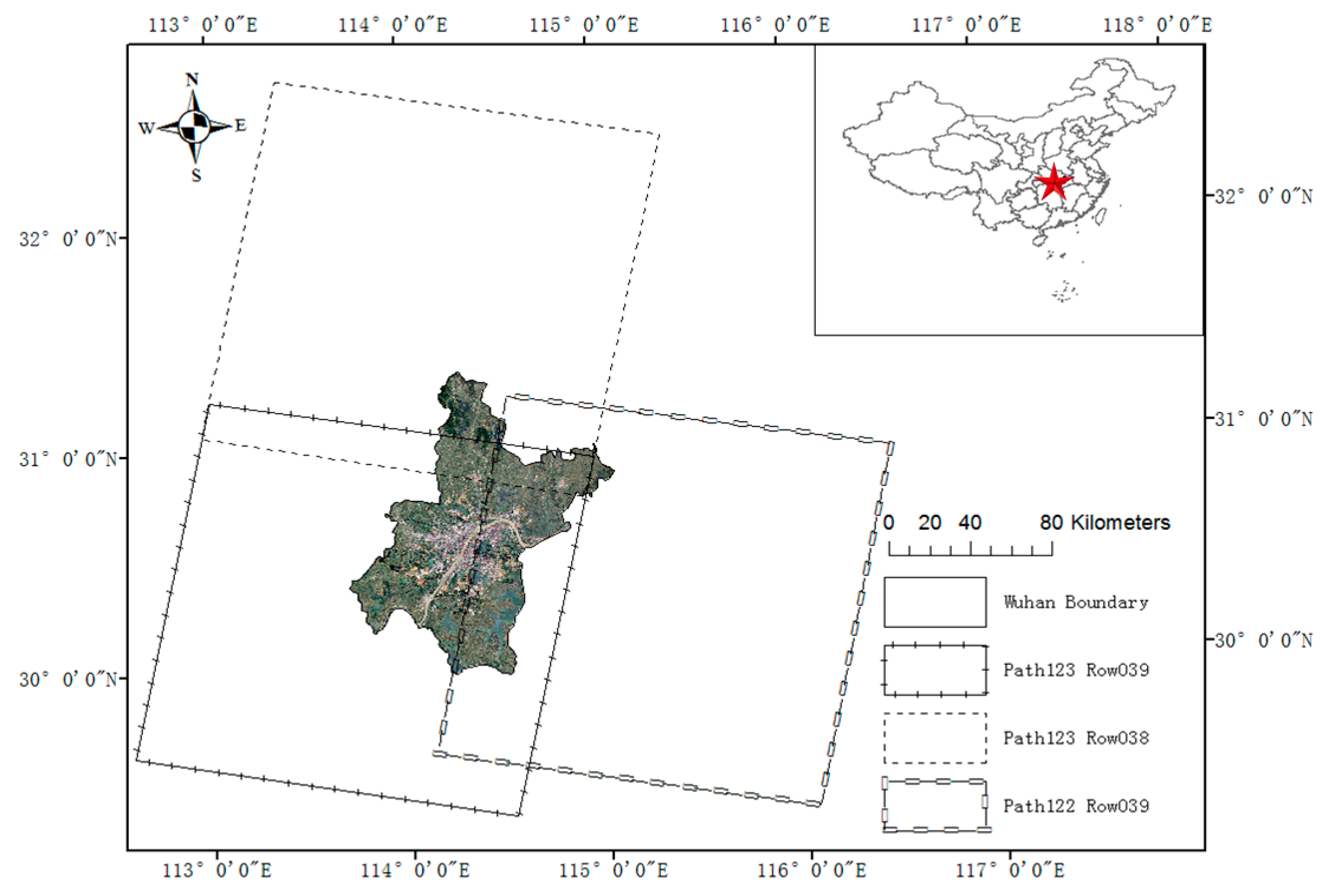
Wuhan city in central China was selected as the study area, which has a geographic location between 29°58′–31°22′N and 113°41′–115°05′E. Wuhan covers 8494.41 km2, and the population grew to 10.77 million by the end of 2016. The study area has a humid subtropical monsoon climate, with a hot rainy summer and a cold wet winter. The terrain is high in the north, and low in the south. Wuhan is the capital of Hubei province, and is also the largest transportation center and the economic center of central China. Due to the “Reform and Opening Up” policy in 1980s, the Chinese society and economy rapidly grew and stimulated urban expansion. As the largest city in central China, Wuhan city experienced a phenomenal social and economic shift that included industrialization and economic growth, and lead to rapid urbanization in the past decades.
Remotely sensed images acquired by the Landsat Thematic Mapper (Landsat 5 TM), the Enhanced Thematic Mapper Plus (Landsat 7 ETM+), and the Operational Land Imager (Landsat 8 OLI) sensors over the period from 1987 to 2016 were used. As shown in
Figure 1, the administrative boundary of Wuhan is located within three scenes (path/row: 123/038, 123/039, 122/039), and most of the study area is covered by the tiles Path123Row039 and Path123Row038. The datasets used in this study were the surface reflectance product generated by using the Landsat Ecosystem Disturbance Adaptive Processing System (LEDAPS) [
40], which was provided by US Geological Survey (USGS) Earth Resources Observation and Science (EROS) Center Science Processing Architecture (ESPA) on demand interface (
https://espa.cr.usgs.gov/). All Landsat time-series datasets were registered to the WGS84/UTM Zone 49N coordinate system when ordering data from the website.
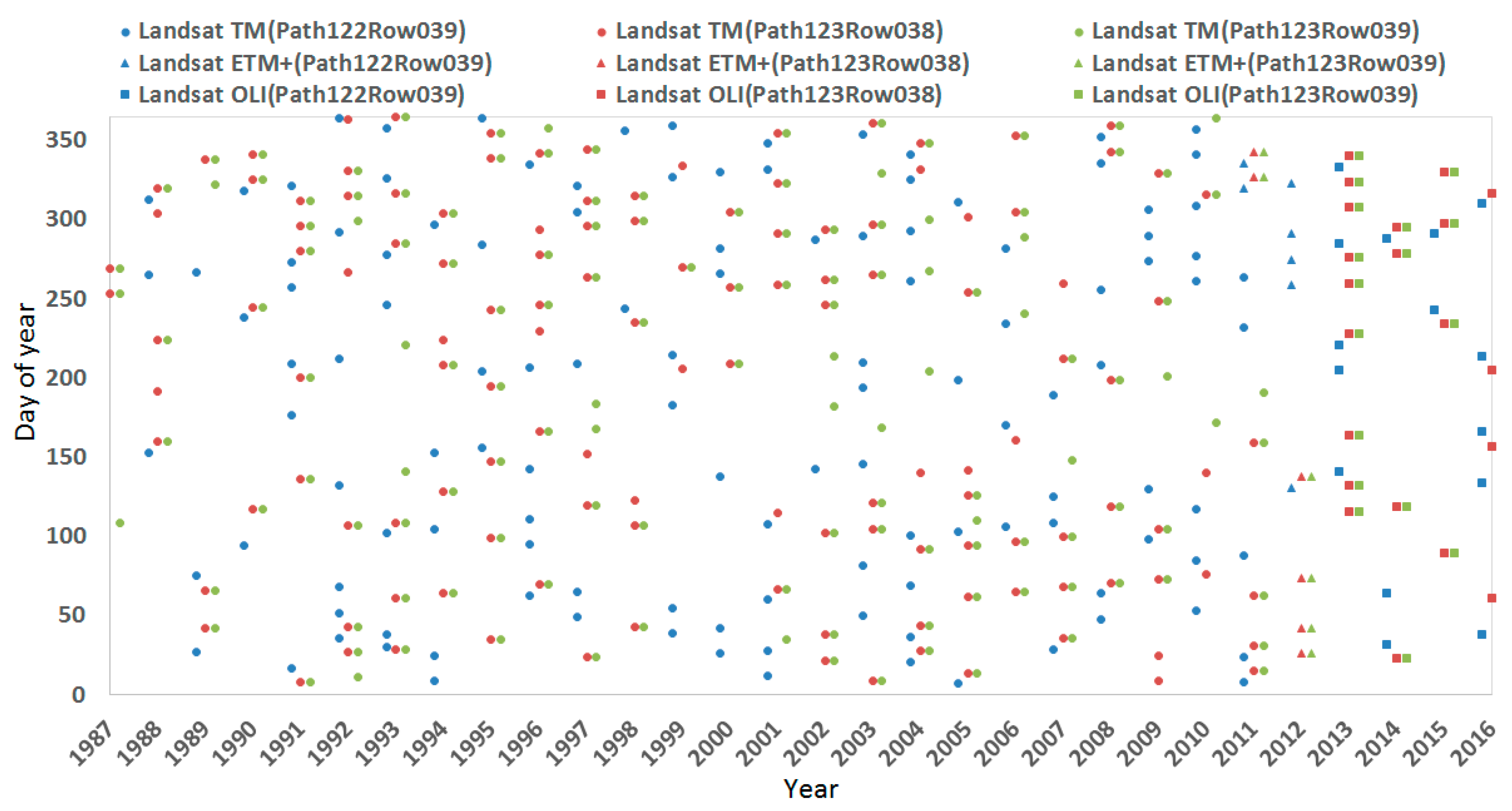
Given that the Landsat 7 ETM+ image has had the scan-line corrector off (SLC-off) problem since 2003, we tried to avoid it, unless it was the only choice in a certain year. Overall, 470 Landsat scenes, including 389 Landsat 4–5 TM scenes, 19 Landsat 7 ETM+ scenes, and 62 Landsat 8 OLI scenes, were collected.
Figure 2 shows the temporal distribution of Landsat scenes used in this study.
2.2. Data Preprocessing
For each Landsat scene, the downloaded data product includes the surface reflectance files of all bands, and the mask file of cloud and shadow. All of the data preprocessing steps were completed in ENVI 5.1 software. Firstly, the Landsat scenes were masked by the corresponding mask file of cloud and shadow. Secondly, as the administrative boundary of Wuhan is located within three Landsat scenes, the three scenes acquired on the same day, or close dates were mosaicked. The mosaic parameters were set as follows: the background value was set as 0; the feathering distance was set as 0; and the color balancing was set as ‘NO’. Then, there were several mosaic images in different dates for every year. Thirdly, all of the mosaic images in the same year were stacked into one image. Finally, all of the stacked images were clipped by the administrative boundary of Wuhan city, and used as input to the classifier to map the land cover.
The cloud, shadow and scan-line corrector off (SLC-off) data would lower the data quality and affect the accuracy of image classification. In this study, although the gaps caused by cloud, shadow, and SLC-off appeared in different locations within the clipping images acquired in the same year, no gap filling method was used. This is mainly because the dense time-series data acquired in the same year can make up most of the gaps for each other, and uncertainty should be brought by gap-filling methods. Therefore, for each year, surface reflectance values in all of the available images were used in the classification, and these gaps were not included during the classification procedure.
2.3. Methods
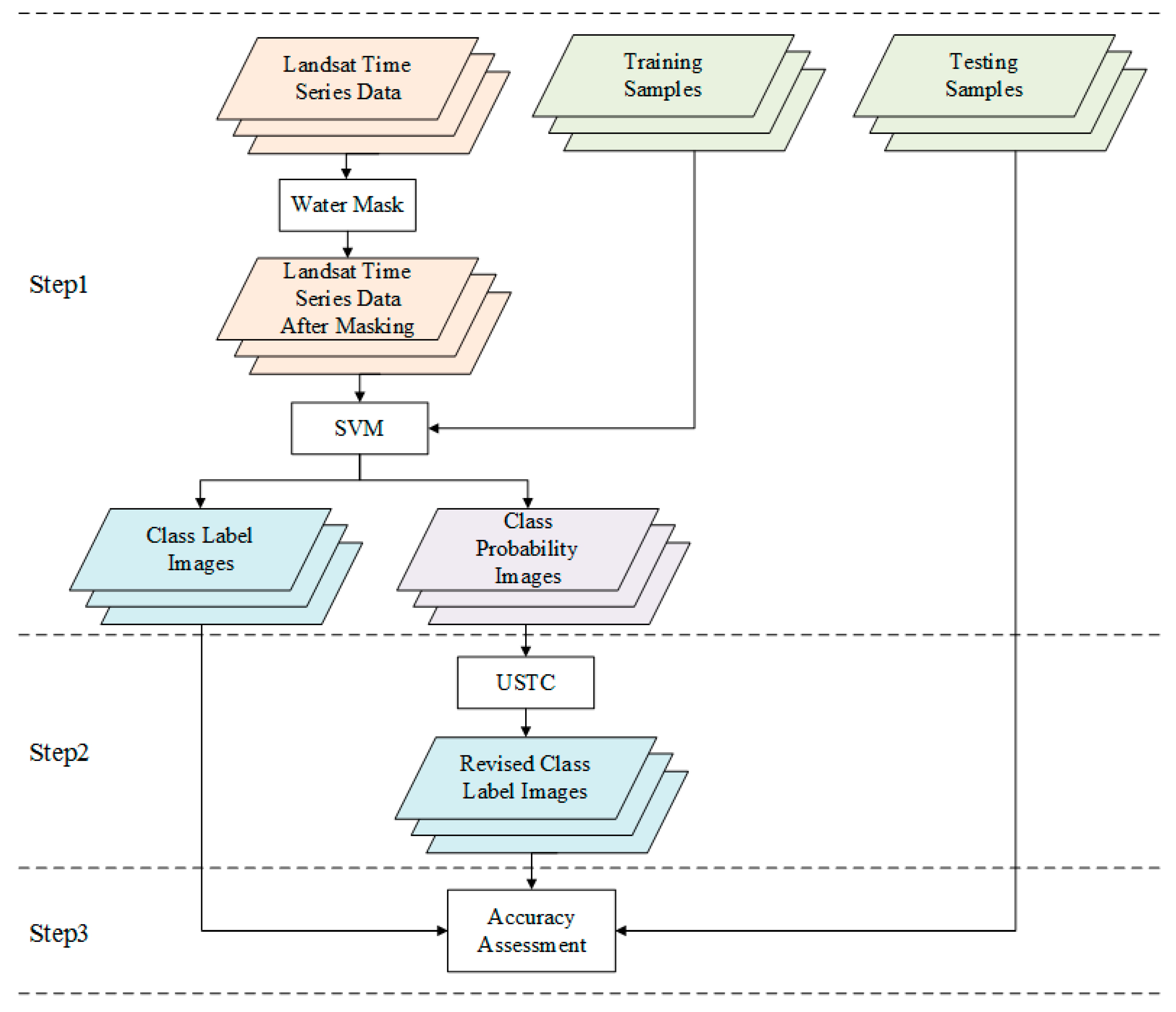
In this study, the spatial-temporal change of impervious surfaces was mapped using the dense time-series Landsat images through the three main steps, as shown in
Figure 3. The first step is the classification of the remotely sensed imagery. The second step is the application of the USTC model, and the last step is the accuracy assessment.
2.3.1. Support Vector Machine Classifier
Support vector machine (SVM), which has been widely applied in remotely sensed image classification with a good performance [
41], was selected as the classifier in our study. According to the vegetation-impervious surface-soil (V-I-S) model [
42], a classification scheme of three land cover classes—vegetation, impervious surface, and soil—was adopted in the SVM classifications. Hence, the water bodies in Wuhan city needed to be removed before doing the SVM classifications.
Lakes and rivers occupy nearly 20% of Wuhan city. In order to reduce the effect of water on classification, the modified normalized difference water index (MNDWI) was used to remove water bodies [
43]. As all of the Landsat images within a year were stacked into one image, the stacked image contained images acquired in different seasons of a year, which lead to different water surface areas. In order to simplify the extraction of the water mask, the rain season, which had the maximum water area, was selected to produce the water mask. The MNDWI was calculated from the Landsat image acquired in the rain season (such as July and August in Wuhan city) as closely as possible, and the water mask was produced by the histogram thresholding method [
44] using the water and non-water samples.
Google Earth imagery was used as the main source of the training samples selection. Since no fine resolution imagery is available for the period from 1987 to 1999, the training samples were also selected from time-series Landsat images using visual judgments. Since the spectral separability of the impervious surface from other classes was maximized in summer [
34], the visual judgments of collecting training samples depended on the false color composite Landsat images were acquired in summer or close to summer for each year. Finally, the training samples and the Landsat images were input to the SVM classifier to get the class label image and class probabilities for each year. Only gaps-free pixels were inputted to the classifier, as the Landsat stacked images may have gaps-free pixels and gaps-included pixels in the same position. In all, 100,097 training samples (including 29,776 impervious surface training samples, 40,778 vegetation training samples, and 29,543 soil training samples) were selected. Then, 30 SVM classifiers were trained with each year’s training samples, and the parameters were set as follows: kernel type was radial basis function; gamma in kernel function was 0.167; penalty parameter was 100.
2.3.2. Classification Uncertainty
In the classification process of remotely sensed images, classification uncertainty can be interpreted as a localized and quantitative measure of doubt in the final class decision on a case-by-case basis [
45,
46]. Measures such as the posterior probability of membership to the allocated class are often used as an indicator of uncertainty on a case-by-case basis in remote sensing [
47]. Hence, the pixel-level classification uncertainty can be measured by class probability vectors [
48].
A popular method for measuring the uncertainties underlying a remote sensing classification is the Shannon–Wienner index [
48,
49,
50]. It is based on communication theory, and can be calculated as [
51]:
where
is the Shannon–Wienner index of the pixel at the position
; and
i, j represent the spatial position of the target pixel;
represents the corresponding time point of target pixel;
is the class label, and
indicates the probability that the pixel
belonging to the
class derived from the SVM classifier. In general, a higher Shannon–Wienner index value indicates a larger uncertainty of the classification result.
In the SVM classifier, a pixel should be assigned to the class label that has the maximum class probability. In this situation, the pixels that have different combinations of class probabilities may be assigned with the same land cover labels. In other words, although some pixels have the same land cover class labels, they have different class probability combinations, which indicate the different class uncertainties of these pixels.
Table 1 shows a simple example, where the V-I-S class probability combination of the first pixel is [0.15, 0.80, 0.05], and that of the second pixel is [0.35, 0.4, 0.25]. According to the SVM classification principle, both pixels should be assigned the same class label: impervious surface. However, the uncertainty of the classification results is different for these two pixels. For the first pixel, the class probability that the pixel belongs to impervious surface is much higher than that of the other classes. For the second pixel, although the probability that the pixel belongs to impervious surface is still higher than those that the pixel belongs to other two classes, their difference is not obvious as that of the first pixel. In this situation, the class label of the second pixel has a higher uncertainty than the first pixel.
2.3.3. Uncertainty-Based Spatial-Temporal Consistency Model
Using the time-series class label images derived by the SVM classifier and the corresponding Shannon–Wienner index as input, the land cover labels were refined by the proposed uncertainty-based spatial-temporal consistency (USTC) model. In order to increase the classification accuracy and the consistency of land cover labels, in the proposed USTC model, both spatial and temporal goal functions are combined to form a single optimization function:
where
is the objective function. The spatial term
aims to match the spatial context information provided by the target pixel and its spatial neighbor pixels. The temporal term includes
and
, which aim to match the temporal context information provided by the target pixel and its temporal preceding and posterior neighbor pixels. The parameter
and
are the adjusting parameters that are used to balance the impact of spatial and temporal terms on the final objective function.
The spatial term is further computed as:
where
I,
J,
T, and
L represent total number of rows, columns, years, and class labels, respectively, for the time-series class label images;
is the spatial neighborhood, which includes all of the pixels inside a square window whose center is the pixel at the position
;
is the size of the square window (e.g.,
square window,
); and
is an indicator function that is equal to 1 if
, and 0 otherwise.
The temporal term is further computed as:
where
and
are the preceding and posterior temporal neighborhood, respectively;
is the class label at the position
; and
is the temporal transition probability from
to
which is calculated by the whole class label images of two consecutive years.
The object of the USTC model is to make the final class label have the maximum posterior probability. The objective function as shown in Equation (2) is used here to make the minimal energy value contribute the maximal posterior probability. The iterated conditional modes (ICM) algorithm [
52] was utilized to maximize the conditional posterior probability of each pixel. In the initialization step, the time-series class label images derived from the SVM classifier for each year from 1986 to 2016 was used as input. The algorithm terminates when the minimum value of the objective function is obtained (i.e., the previously fixed number of iterations is achieved, or less than 0.1% of the land cover labels are changed across two iterations). At last, classification results with three class labels (i.e., vegetation, impervious surface, and soil) produced by the USTC model were translated into classification results with binary class labels (i.e., impervious surface and pervious surface) by combining the classes for accuracy assessment.
Meanwhile, the TC model [
34] proposed by Li et al. was selected as a contrast to the proposed USTC model. The TC model involves temporal filtering and logic reasoning. In terms of temporal filtering, the temporal consistency probability is calculated based on a predefined temporal window size. Then, the class label is obtained based on a simple rule regarding the temporal consistency probability’s threshold. In terms of logic reasoning, it is applied to modify the misclassification noises after temporal filtering.
2.3.4. Accuracy Assessment
The impervious surface classification results derived by the SVM classifier, the TC model, and the proposed USTC model were assessed using not just the overall accuracy (OA), but producer’s accuracy (PA) and user’s accuracy (UA) also. Unlike the training samples used in the SVM classifier, the testing samples used in accuracy assessment contained only two classes: impervious surface class and pervious surface class. In this study, the testing samples were collected based on the “stratified random sampling” rule [
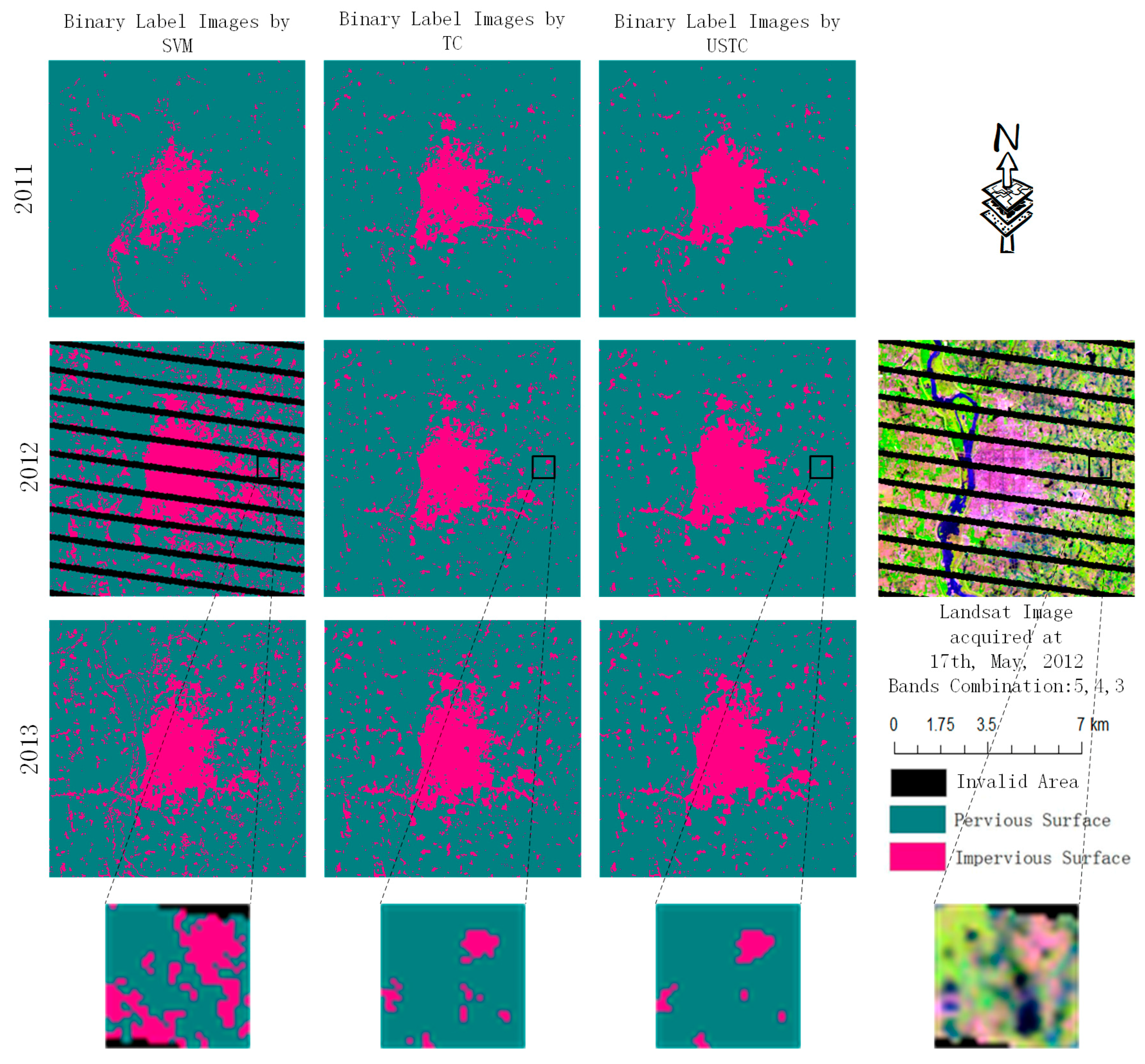
53]. In all, 3714 impervious surface testing samples and 5940 pervious surface testing samples were randomly collected. Then, the annual OA, PA, and UA were produced. Besides the quantitative accuracy comparison, the visual accuracy comparison of various approaches was also applied. Three subareas located in the main urban areas of Jiangxia, Huangpi, and Xinzhou districts were selected to compare the results produced by different methods, in order to make the visually comparison more clearly.
3. Results and Discussion
3.1. Classification Results
These subareas (i.e., Jiangxia, Huangpi, and Xinzhou districts) represent three different cases of classification results derived by the SVM classifier; that is, the overestimation of impervious surface, the underestimation of impervious surfaces, and the invalid area where the class labels were not determined. There are some possible reasons for this issue, such as for example, the quality of Landsat images, the training sample selection, spectral confusions among different cover types, the season characteristics of Landsat images, and other uncertainty factors in the classification process. Then, the comparison of three classification results derived by the SVM classifier, the TC model, and the USTC model was shown visually (
Figure 4,
Figure 5 and
Figure 6) and numerically (
Table 2).
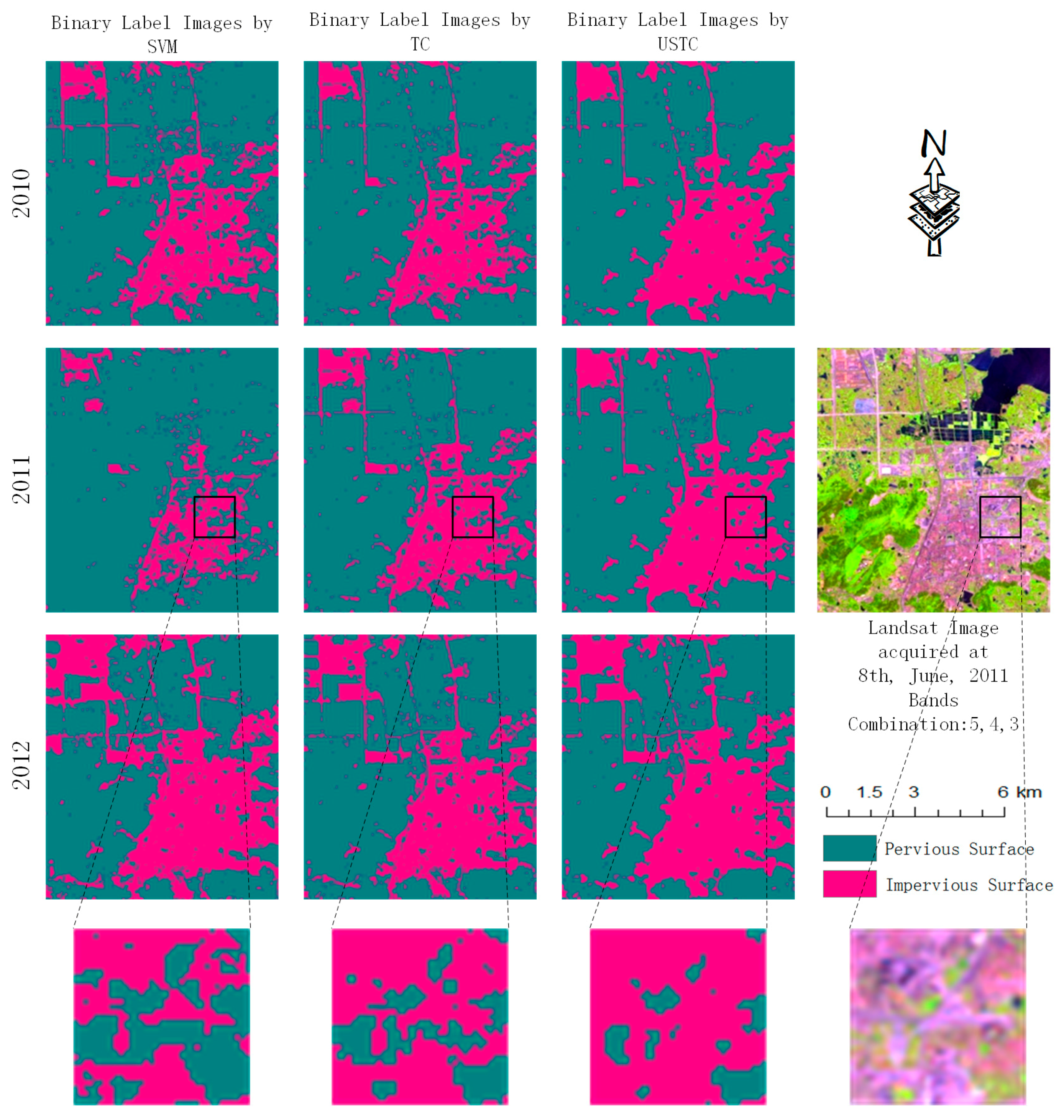
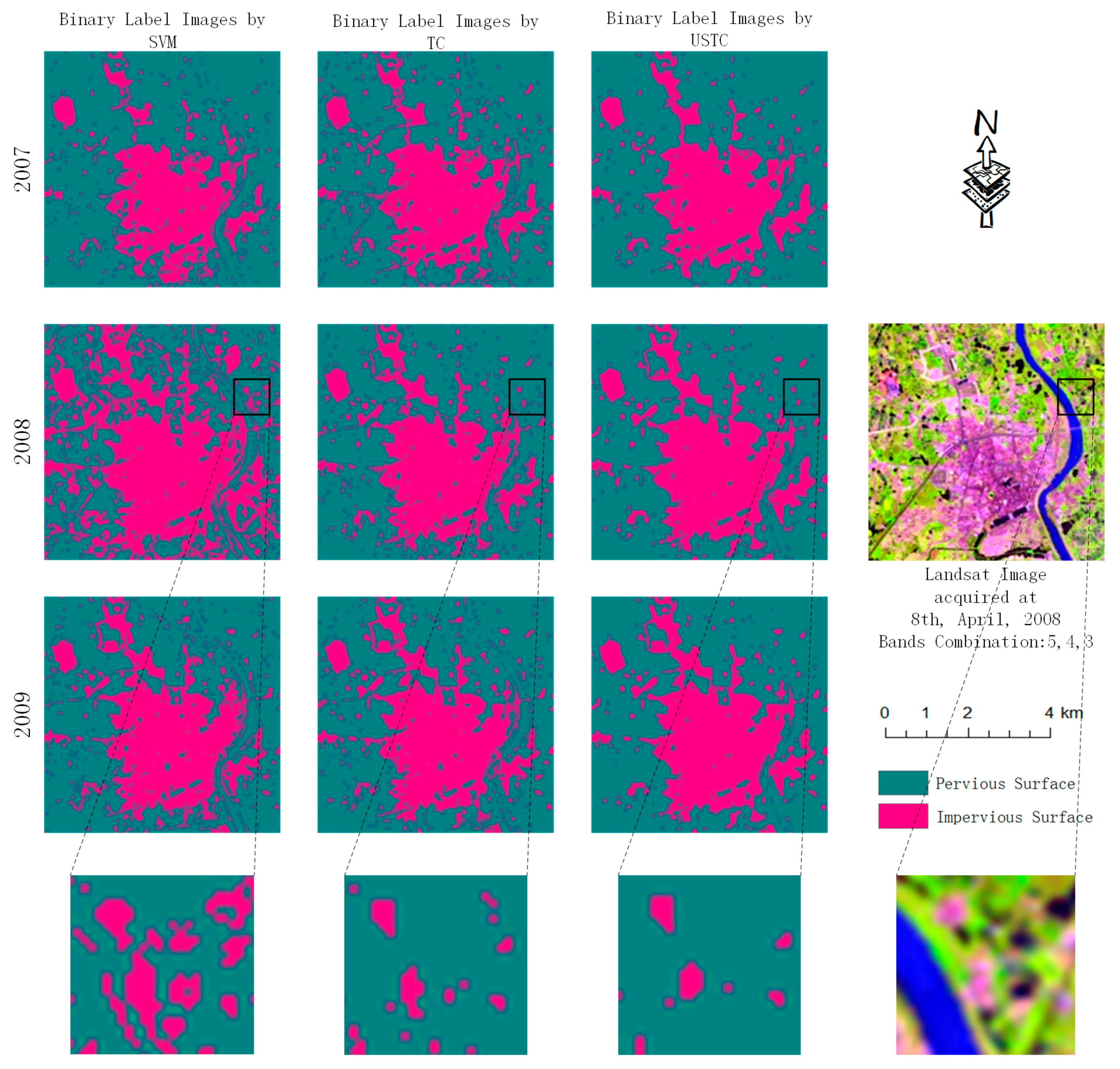
Figure 4 shows the case in which the impervious surfaces were overestimated by the SVM classifier. Compared with impervious surfaces in 2007 and 2009, impervious surfaces estimated by the SVM classifier had a sudden increase in 2008. Generally, from the view of the characteristics of urban expansion, the sudden increase of impervious surface in a three-year sequence is possibly illogical. Hence, this phenomenon was most likely caused by the misclassification of the SVM classifier. After applying the TC model and the proposed USTC model, the overestimated area was much reduced, and the classifications in the three-year sequence were more in line with the characteristics of urban expansion. Through comparing the classification results, it was found that the classification result produced by the USTC model was more aggregated than the classification result produced by the TC model. In the view of amplified images in black box, the classification result produced by the USTC model is closer to the reference image than that produced by the TC model, especially in regards to the visual classification of tiny impervious surface patches.
Figure 5 shows the case in which the impervious surfaces were underestimated by the SVM classifier. Similar to the overestimation case, the sudden increase of impervious surface in a three-year sequence is also considered to be illogical. By applying the TC model and the USTC model, many areas misclassified as pervious surfaces were relabeled to be impervious surfaces. In contrast with the TC model, similarly, the USTC model had advantages in impervious surface aggregation and modification of the tiny impervious surface patches clustered by misclassification. From the amplified images in black box, it is found that the USTC model performs best, with the TC model performing second best, and the SVM classifier performing worst in the classification results. In addition, the USTC model performed better than the TC model in the spatial-temporal consistency of impervious surfaces visually, especially for some small patches, such as roads.
Figure 6 shows the case in which there is an invalid area in the SVM classification result. The invalid area is caused by gaps such as clouds, shadows, and SLC-off, etc. Here, the gap caused by Landsat ETM+ SLC-off is used as an example. By applying the TC model and the USTC model, the gap can then be restored by using the spatial-temporal neighboring land cover labels. Most of the gaps in the SVM classifier results were well revised by both the TC and USTC models. In the view of amplified images in black box, the USTC model corrects more misclassifications than the TC model and the SVM classifier. It also can be noticed in the figure that the USTC model performed better than the TC model in terms of the spatial-temporal consistency of impervious surfaces visually.
Table 2 shows the confusion matrixes derived by the SVM classifier, the TC model, and the USTC model. All of the testing samples were used to compute the confusion matrix for all of the years. In contrast to the confusion matrix of the SVM classifier, the numbers on the main diagonal in the confusion matrix of the TC model or the USTC model increased, which indicated that both the TC model and the USTC model were effective in improving the classification accuracy. Through comparing the confusion matrixes of the TC model and the USTC model, it is noticed that the impervious surface number on the diagonal in the confusion matrix of the USTC model increased greater than that in the confusion matrix of the TC model. This indicated that the USTC model performed better than the TC model in the improvement of impervious surface classification accuracy. However, it is also noticed that the pervious surface number on the diagonal in the confusion matrix of the USTC model was exactly the opposite, meaning that the TC model performed better than the USTC model in the improvement of pervious surface classification accuracy. That is probably due to the different processing operations of class labeling in the two models. The vegetation label and soil labels were converted to the pervious surface label before being inputted into the TC model; however, the USTC model took the original class labels as input. As a whole, the USTC model got a considerable improvement in the overall accuracy (OA), of about 4.23% above that of the SVM classifier, and an improvement of about 1.79% above that of the TC model. Therefore, these improvements in accuracy indicated that incorporating the uncertainty information of the classification was useful for improving the time-series classification results.
In addition,
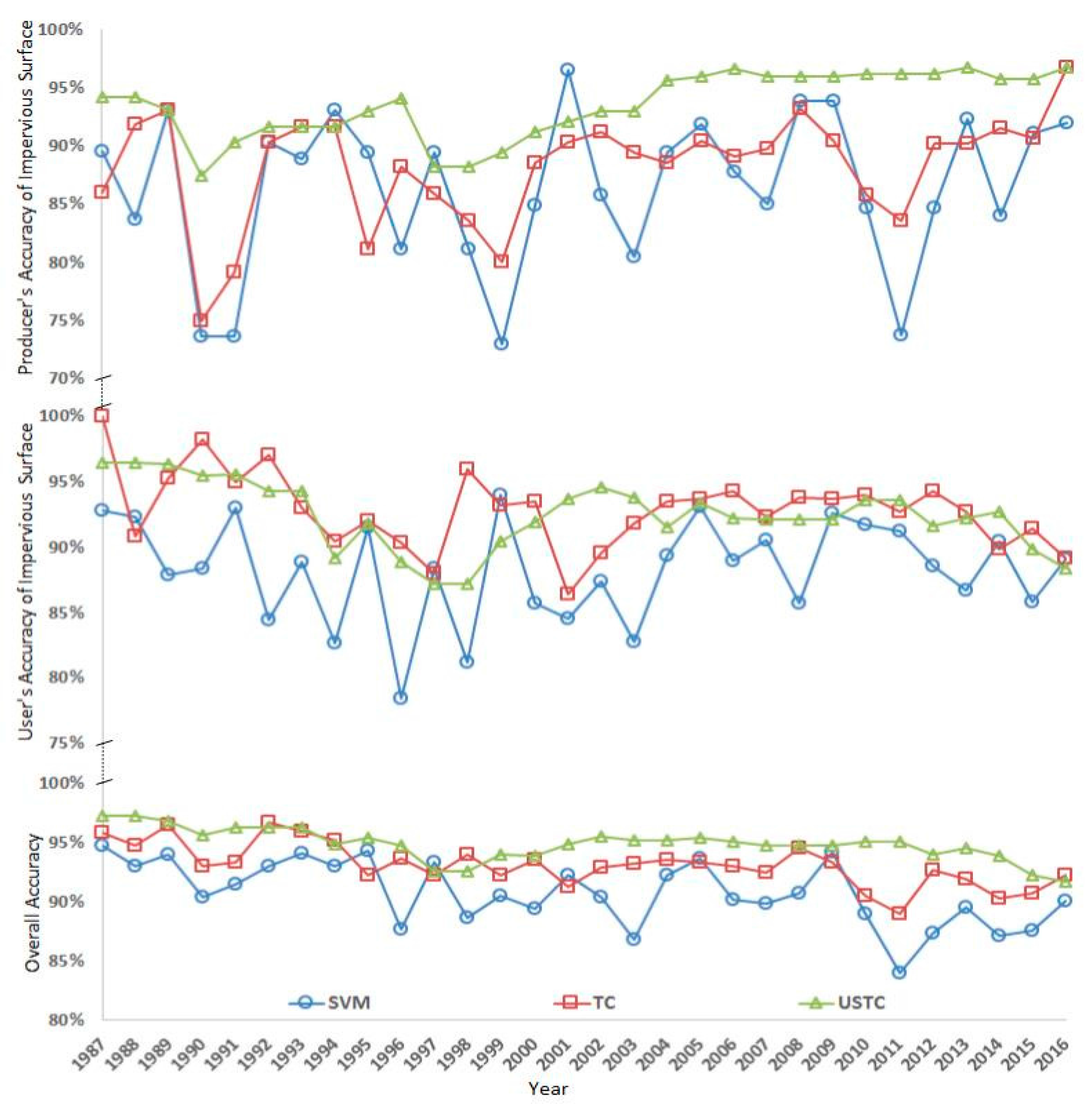
Figure 7 shows the accuracy comparison (i.e., PA, UA, and OA) of three classification results derived by the SVM classifier, the TC model, and the USTC model. In terms of the impervious surface’s user accuracy and producer accuracy, it was found that, similar to the result of the overall accuracy, the USTC model performed best, with the TC model performing second best, and the SVM classifier performing worst in PA. However, in terms of their performance in UA, the TC model (i.e., the average UA is 92.47% in
Table 2) performed better than the USTC model (i.e., the average UA is 92.27% in
Table 2), with a small advantage. In terms of overall accuracy, it varied from 83.99% to 94.72% in the SVM classifier classification result, 90.57% to 96.67% in the TC model classification result, and 91.73% to 97.18% in the USTC model classification result. It is also shown that the USTC model performs best, with the TC model performing second best, and the SVM classifier performing worst in terms of overall accuracy. According to the statistical test results derived by one-way analysis of variance (ANOVA), it was indicated that the USTC model is significantly better than the TC model, which is significantly better than the SVM model (
p < 0.05). Moreover,
Figure 7 shows a descending trend of the values of overall accuracy from 1987 to 2016. This is probably because the urban area expanded during the study period, and the building materials of impervious surfaces were becoming more and more complex in recent years, which may have increased the diversity of the spectral characteristics of the impervious surface, and raised the difficulty of the impervious surface classification. The choice of testing samples may also account for the descending trend. In the end, when taking UA, PA, and OA into consideration together, however, the USTC model performed better than the TC model.
3.2. Annual Change of Impervious Surface
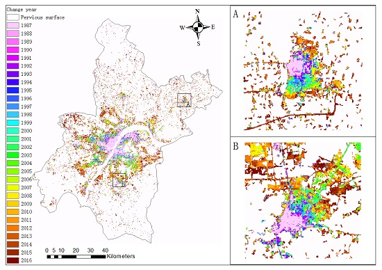
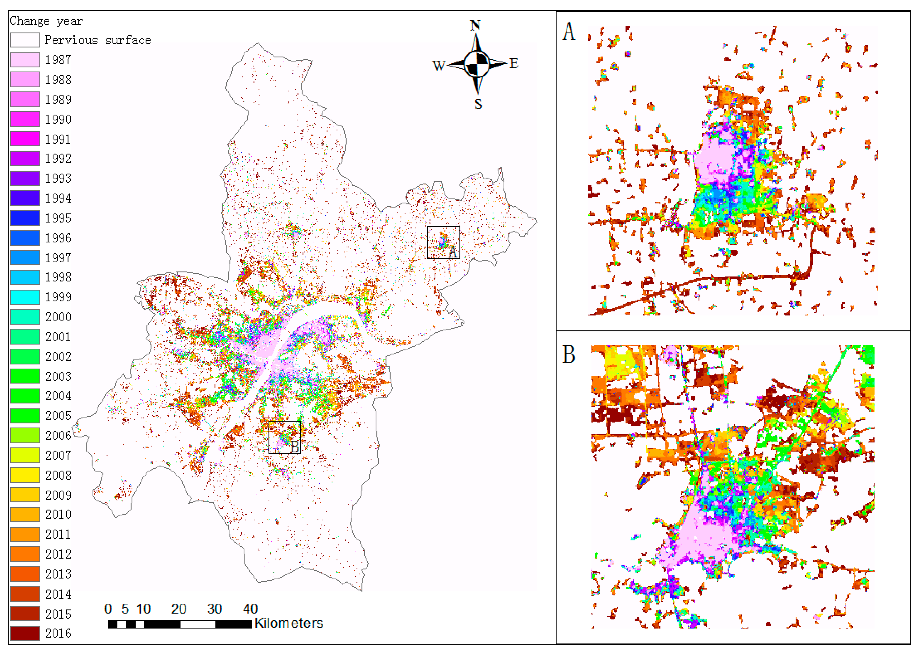
A map of annual impervious surface change was produced to better visualize the process of urban expansion in Wuhan city from 1987 to 2016 (
Figure 8). The white color represented pervious surfaces, including water bodies, and the gradual colors from shallow to deep described the annual change of impervious surfaces. From
Figure 8, it is noticed that Wuhan city had experienced a dramatic urban expansion from 1987 to 2016, and impervious surfaces expanded from urban cores to suburban areas.
Two subareas were selected for a more detailed study of the annual change in impervious surface. Subarea A is located in the northeast of Wuhan city, and it covers the main urban area of Xinzhou district. Subarea B is located in the southeast of Wuhan city, and it covers the main urban area of Jiangxia district. As shown in
Figure 8, in the subarea A, the newly developed urban areas are located in the south part of Xinzhou district, and a road was built in 2015. This road may be built for better catering to urban expansion. In the subarea B, the newly developed urban areas are located in the northeast and northwest parts of Jiangxia district. In 2003, a road was built in the northeast of Jiangxia district. Then, urban expansion began around this road in subsequent years.
The long-term impervious surfaces dataset at an annual frequency provides an opportunity to better understand the spatial-temporal pattern of urban expansion in Wuhan city. In contrast to coarser time intervals (e.g., 5–6 years), the annual frequency can provide a method for capturing the details of land cover change in rapidly developing regions, where the change of urban lands may be considerable over a short period of time (e.g., one to two years). As a fast-growing city, the timely mapping of impervious surface and its change is necessary in order to monitor the urban expansion. With this dataset, it is noticed that in Wuhan city, the road is a very important kind of impervious surface. Road construction is often the foundation and precondition of other impervious surface expansion, while other impervious surface expansion can push road construction forward.
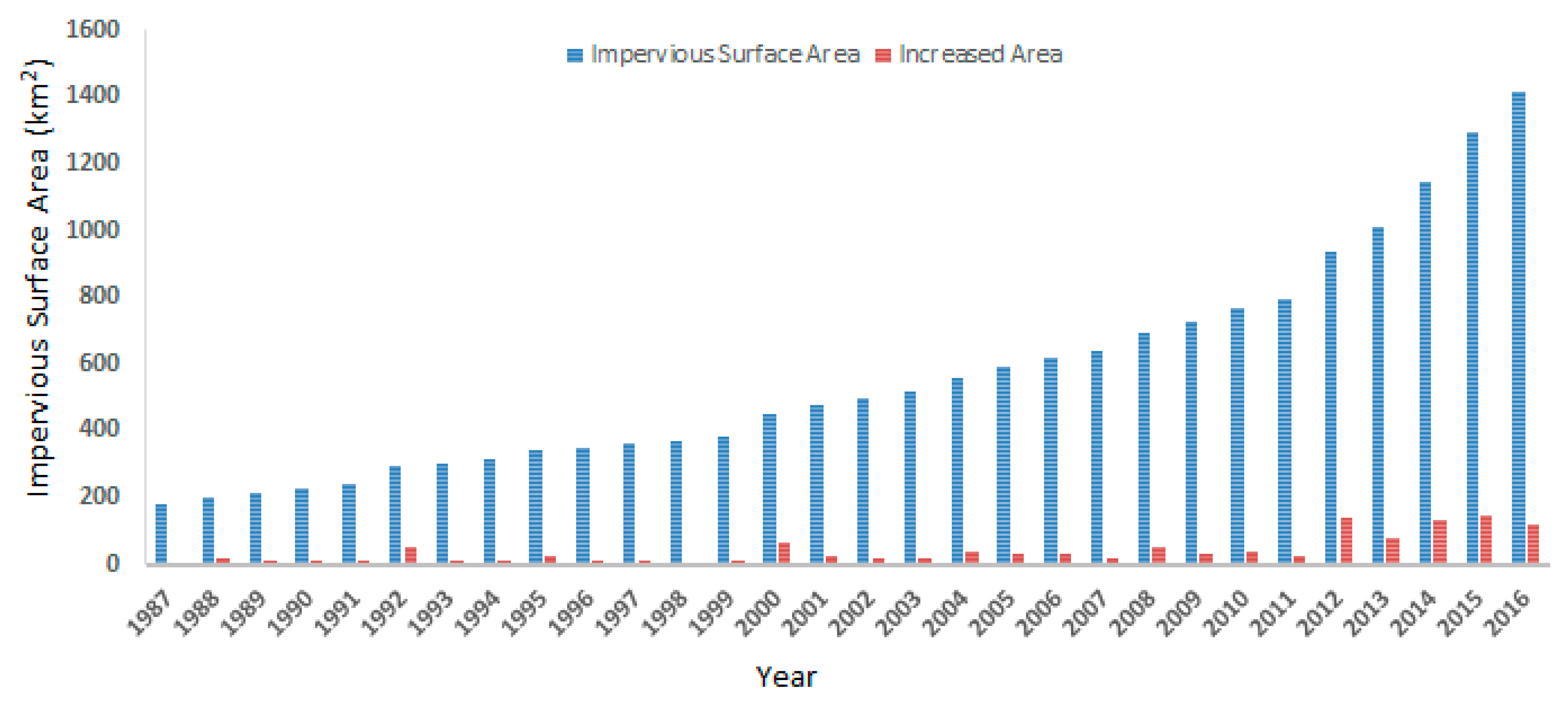
Figure 9 shows the impervious surface area for every year from 1987 to 2016. Impervious surface area increased from 179.75 km
2 in 1987 to 1412.12 km
2 in 2016, yielding at an average annual growth in impervious area of 42.50 km
2. Meanwhile, the increased area, which was calculated by the difference area of the two adjacent years, was also shown in
Figure 9. As the increased area shows, the years of 1992, 2000, and 2012 are the significantly increased timing nodes during the impervious surface expansion. Then, four periods of 1987–1991, 1992–1999, 2000–2011, and 2012–2016 were analyzed for better understanding the annual growth rate in Wuhan city. From 1987 to 1991, Wuhan city experienced its initial expansion. The impervious surface area increased from 2.10% of the total area in 1987 to 2.81% in 1991, at an annual average rate of 7.60%. During the period of 1992–1999, the impervious surface area increased from 3.42% of the total land area in 1992 to 4.50% in 1999, yielding at an annual average rate of 6.22%. Compared with the first period (i.e., 1987–1991), the annual growth rate during the second period (i.e., 1992–1999) declined slightly. During 2000–2011, the impervious surface area increased from 5.27% of the total land area in 2000 to 9.25% in 2011, growing at an annual average rate of 6.25%. The annual growth rate over the third period (i.e., 2000–2011) was roughly equal to the rate over the second period (i.e., 1992–1999). Hence, the first three periods saw a relatively steady growth rate in impervious surface expansion; For the period of 2012–2016, the impervious surface area increased from 10.90% of the total land area in 2012 to 16.48% in 2016, yielding at an annual average rate of 12.29%. It’s clear that the annual growth rate over the fourth period (i.e., 2012–2016) was substantially greater than the rate over the first three periods. The reason for this large increase of impervious surface over the period of 2012–2016 was that Wuhan city carried out main urban optimization and new urban planning based on ‘The Urban Overall Planning of Wuhan City (2010)’, which was provided by the Wuhan Land Resource and Planning Bureau. In response to the ‘The Middle Area Rise Strategy’, Wuhan city is vigorously implementing the “industrial multiplication” plan. Due to the rapid development of the industry, a large amount of residential houses have been built in the expanding urban area. Moreover, the transformation of the urban core stimulated industrial economic development in the urban fringe. Meanwhile, large-scale infrastructure projects, including main roads, ring roads and outer ring highways, subways, and a high-speed railway line have been constructed or are under construction. Hence, we can infer that Wuhan city has recurrently experienced rapid urbanization.
3.3. Impervious Surface Expansion At Different Directions
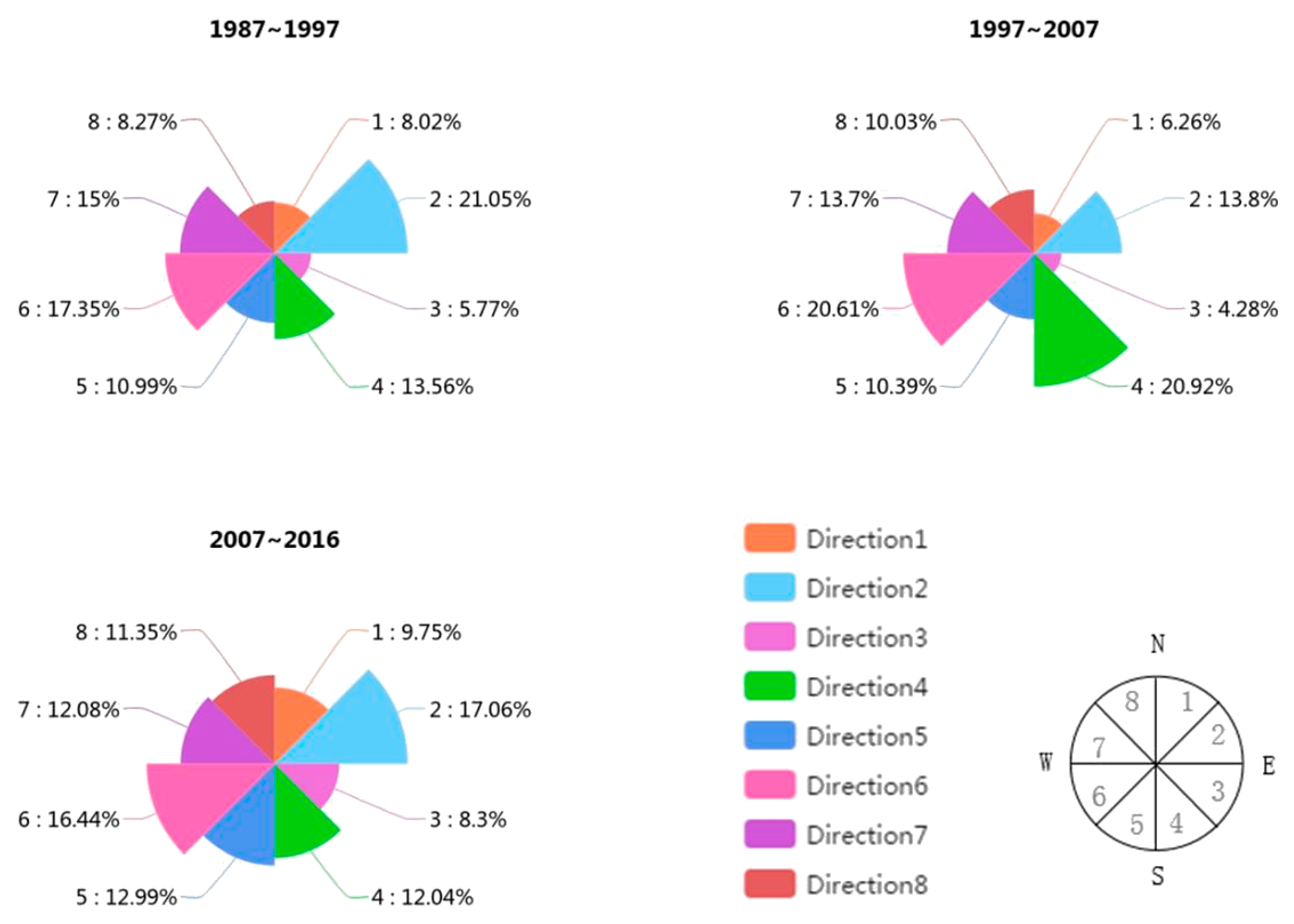
Figure 10 shows impervious surface expansion in eight directions during three periods: 1987–1997, 1997–2007, and 2007–2016. The expanded area of impervious surface was calculated by the subtraction of the starting time and the ending time for each period.
From 1987 to 1997, the fastest-growing direction of impervious surfaces was Direction 2 (i.e., east by north 45°). The second fastest-growing direction was Direction 6 (i.e., west by south 45°). These two directions form the fastest-growing diagonal. Moreover, both of them account for 48.40% of the total impervious surface growth area. That is mainly because the idea of transportation and circulation development was put forward in the ‘The Urban Overall Planning of Wuhan City (1988)’. Then, public service facilities and infrastructure construction were built, such as Hankou railway station, Wuhan passenger transport port, Tianhe airport, and a lot of freight stations. These constructions centered on the old urban area, which is located on both sides of the Yangtze River.
From 1997 to 2007, the fastest-growing direction was Direction 4 (i.e., south by east 45°), which accounts for 20.92% of the total impervious surface growth area. The second fastest-growing direction was Direction 6 (i.e., west by south 45°), which has a small disadvantage compared with Direction 4. In contrast to the first period, the second period has some fluctuations in eight directions, in terms of impervious surface expansion. For example, the ratio of Direction 2 has declined by 7.25% between the first period and the second period, but the ratio of Direction 4 has increased by 7.32% between the first period and the second period. That’s mainly because the ‘The Urban Overall Planning of Wuhan City (1996)’ put forward the idea of the construction of satellite towns. Hence, some towns located in the peripheral urban area were in construction in order to evacuate some of the population in the main urban area. Jiangxia district got a big urban expansion due to its convenient traffic conditions, and the new developed urban area in Jiangxia district is mainly located along the Huyu expressway. At the same time, the Dong Hu High-tech Industrial Development Zone authorized by the central government in 1991 had attracted a large amount of investment for high-tech firms, the automobile industry, and other large scale manufacturing industries. Both of them are located along Direction 4 (i.e., south by east 45°). Hence, the fastest-growing direction is Direction 4 (i.e., south by east 45°) over the period 1997–2007.
During 2007–2016, Direction 2 was once again the fastest-growing direction, and Direction 3 was the slowest-growing direction through the entire time. In contrast to the first two periods, however, the third period had a more uniform growth of impervious surface in all eight directions. That’s mainly because Wuhan city had been upgraded to the level of national development strategy on the background of ‘The Middle Area Rise Strategy’. Hence, ‘The Urban Overall Planning of Wuhan City (2010)’ put forward the idea of main urban optimization and new urban planning. Meanwhile, Wuhan city is vigorously implementing the “industrial multiplication” plan. These factors greatly stimulated impervious surface expansion.
Through analyzing the directions of impervious surface expansion, some conclusions are derived. Firstly, the relatively faster-growing directions of Wuhan city are east by north 45° (Direction 2), and west by south 45° (Direction 6). The two directions form a diagonal, which impervious surface expanded around. It is also noticed that the two directions just matched the flow direction of Yangtze River in Wuhan city. Secondly, impervious surface expansion was initially uneven (during the first two decades), and then relatively even (during the last decade). Under the stimulus of the economy and population growth, urbanization is now speeding up on all available land. For this reason, the impervious surface expansion was relatively even in all directions over the 2007–2016 period, which shows that a serious urbanization is occurring in Wuhan city. This would lead to many urban environmental problems. Hence, further development should focus on the environment and ecology.
4. Conclusions
In this paper, we developed an uncertainty-based spatial-temporal consistency (USTC) model to characterize and quantify the annual spatial-temporal change of impervious surfaces in Wuhan city using time-series Landsat sensor data from 1987 to 2016. Compared with previous temporal models that only used the land cover labels produced by a classifier, we regarded the uncertainty of classification as an indicator for evaluating the attribution of the spatial-temporal neighboring pixels to the target pixel. The experimental results showed that the proposed USTC model performed better than the SVM classifier and the TC model in terms of classification accuracy. The proposed USTC model made the resultant land cover maps more consistent, and the overall accuracy of the proposed USTC model had an increase of 4.23% over that of the SVM classifier, and an increase of 1.79% over that of the TC model, which showed the effectiveness of the proposed USTC.
The experiment results also indicated that the impervious surface area in Wuhan city increased rapidly, from 2.1% of the total land area in 1987 to 17.93% in 2016, with the growth from urban cores to suburban areas. The contributions of this study are in the following aspects. First, the annual mapping of the impervious surface area from 1987 to 2016 for Wuhan city demonstrate that time-series Landsat data can provide valuable urban development information for urban growth modeling and the monitoring of urban planning effects. Second, this study showed how class membership uncertainty can be used to increase classification accuracy in time-series images.
Further enhancement to the mapping of land cover change in time-series data may be made. Temporal transition probability, as an important parameter involved in the USTC model calculation, is critical for accurately estimating the temporal transition probability with a more effective method than the wall-to-wall statistics of temporal neighbors. Different methods can be used to estimate the temporal transition probabilities, such as Bayesian calibration, and the uniform asymptotic method. Moreover, an increasing number of remotely sensed data will be freely available upon the rapid development of remote sensing technology. However, only Landsat time-series datasets were employed in this study. In future studies, we will test our model over a larger area, and use other remotely sensed data to broaden its application.

 ,
, 


