Assessment of In-Season Cotton Nitrogen Status and Lint Yield Prediction from Unmanned Aerial System Imagery


1
Centre for Regional and Rural Futures (CeRRF), Deakin University, Griffith, NSW 2680, Australia
2
Yanco Agricultural Institute, Department of Primary Industries (DPI), Yanco, NSW 2703, Australia
*
Author to whom correspondence should be addressed.
Remote Sens. 2017, 9(11), 1149; https://doi.org/10.3390/rs9111149
Submission received: 18 September 2017
/
Revised: 27 October 2017
/
Accepted: 6 November 2017
/
Published: 8 November 2017
(This article belongs to the Section Remote Sensing in Agriculture and Vegetation)
Abstract
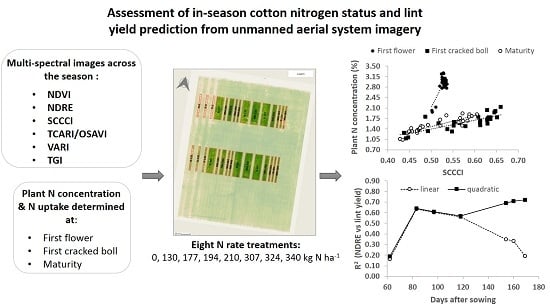
:The present work assessed the usefulness of a set of spectral indices obtained from an unmanned aerial system (UAS) for tracking spatial and temporal variability of nitrogen (N) status as well as for predicting lint yield in a commercial cotton (Gossypium hirsutum L.) farm. Organic, inorganic and a combination of both types of fertilizers were used to provide a range of eight N rates from 0 to 340 kg N ha−1. Multi-spectral images (reflectance in the blue, green, red, red edge and near infrared bands) were acquired on seven days throughout the season, from 62 to 169 days after sowing (DAS), and data were used to compute structure- and chlorophyll-sensitive vegetation indices (VIs). Above-ground plant biomass was sampled at first flower, first cracked boll and maturity and total plant N concentration (N%) and N uptake determined. Lint yield was determined at harvest and the relationships with the VIs explored. Results showed that differences in plant N% and N uptake between treatments increased as the season progressed. Early in the season, when fertilizer applications can still have an effect on lint yield, the simplified canopy chlorophyll content index (SCCCI) was the index that best explained the variation in N uptake and plant N% between treatments. Around first cracked boll and maturity, the linear regression obtained for the relationships between the VIs and both plant N% and N uptake was statistically significant, with the highest r2 values obtained at maturity. The normalized difference red edge (NDRE) index, and SCCCI were generally the indices that best distinguished the treatments according to the N uptake and total plant N%. Treatments with the highest N rates (from 307 to 340 kg N ha−1) had lower normalized difference vegetation index (NDVI) than treatments with 0 and 130 kg N ha−1 at the first measurement day (62 DAS), suggesting that factors other than fertilization N rate affected plant growth at this early stage of the crop. This fact affected the earliest date at which the structure-sensitive indices NDVI and the visible atmospherically resistant index (VARI) enabled yield prediction (97 DAS). A statistically significant linear regression was obtained for the relationships between SCCCI and NDRE with lint yield at 83 DAS. Overall, this study shows the practicality of using an UAS to monitor the spatial and temporal variability of cotton N status in commercial farms. It also illustrates the challenges of using multi-spectral information for fertilization recommendation in cotton at early stages of the crop.
1. Introduction
Nitrogen (N) fertilization management is essential in sustaining cotton productivity and profitability [1]. As with many crops, newer high-yielding varieties require high amounts of N fertilizer and consequently, the N fertilizer demand is expected to increase worldwide during the coming years [2]. N fertilization is important in cotton production because less than an optimal supply of this nutrient can lead to a reduction in lint and seed yield [3]. In contrast, excessive N supply may also increase the cost of production and reduce profitability due to detrimental effects on lint yield and may contribute to environmental N pollution [4]. Optimized N fertilization strategies have been emphasized as being essential to mitigate the emissions of the greenhouse gas nitrous oxide (N2O) at the field level and consequential environmental impacts [5].
In-season assessment of crop N status is a highly recommended practice in cotton production to fit N inputs to the actual crop requirements. The conventional method employed for in-season crop N status assessment in cotton has been the chemical analysis of either petioles or leaf blade samples randomly taken from different areas of each cotton field [6,7]. However, this method is destructive, time-consuming and expensive, and therefore, alternative techniques have been explored during the last years to track crop N status. Remote sensing of crops by means of sensors that can be installed in a variety of platforms such as hand-held devices, tractors, unmanned aerial systems (UASs) or satellites has shown potential for tracking spatial and temporal variability of crop nutrient status [8].
1.1. Sensitive Wavebands to Crop Nitrogen Deficiency
Spectral reflectance characteristics of N deficient plants differ from those of plants at optimum levels, particularly at specific wavelengths. Therefore, reflectance measurements have the potential to be used for in-season crop N status assessment. Experiments conducted in the last decade using ground sensors at field and canopy level have evaluated the feasibility of different single or combined vegetation indices (VIs) to track N deficiencies in cotton. Buscaglia and Varco [9] reported that reflectance at 550, 612, 700, and 728 nm wavelengths at the leaf level were well correlated with cotton leaf N concentration, which is considered to be a good indicator of in-season cotton N status [1]. The red edge band is the transition region of the reflectance between the red and near infrared (NIR) regions. Tarpley et al. [10] and Read et al. [11], showed that at leaf level, ratios combining wavebands of the red edge and NIR region provided a good prediction of total leaf N concentration. Read et al. [11], however, found differences between leaf and canopy (1 m above canopy) measurements in the wavelength range most sensitive to plant N status, with the latter showing the highest correlations. More recently, in an experiment using a ground-based sensing system (1.93 m above the ground), Raper and Varco [12] showed that indices using reflectance in the red edge region correlated more strongly to leaf N status and total plant N content than indices relying on reflectance in green or red regions. These authors [12], suggested further exploration of the simplified canopy chlorophyll content index (SCCCI), for which the calculation requires reflectance at three wavelengths (including reflectance in the red edge band), as an indicator of total N content in cotton.
The normalized difference vegetation index (NDVI) has been reported as a useful index to monitor within-field variability and growth in different crops [13]. Since sufficient N availability ensures plant growth, monitoring the variation in canopy structure (biomass) by remote sensing may provide indirect estimations of crop’s N status. In cotton, experiments with ground-based sensing systems have shown that NDVI is more sensitive to changes in plant height and biomass than to leaf N status. Thus the use of indices more sensitive to chlorophyll content have been recommended instead for assessing crop N status [14]. The opposite has been reported regarding prediction of lint yield. Indices sensitive to plant biomass have performed better than those sensitive to chlorophyll content at stages of the crop when fertilizer application can still have some effects on crop performance [15,16,17]. Zarco-Tejada et al. [16], in an experiment carried out in cotton in which an airborne campaign was conducted (1500 m altitude; 1 m pixel resolution), obtained good correlations between lint yield and NDVI measurements taken at early-mid season. Red edge-based indices, on the other hand, did not perform well at early- to mid-stages of the crop and were only correlated with yield at late stages. Similar results were obtained by Zhao et al. [17] who used a portable spectroradiometer to take spectral measurements in a cotton experimental site. These authors reported that NDVI was associated with relative lint yield at any growth stage between pre-flowering and first boll opening, being the early flower stage (70–75 DAS in that case) the period when the best yield predictions were obtained.
1.2. Unmanned Aerial Systems for Monitoring Crop Performance
Despite the fact that studies on remote sensing of crop N status in cotton have been widely reported in the literature, the vast majority of these studies have been focused on the use of ground-based sensors (hand-held spectroradiometers or tractor platforms). During the last two years, however, there has been a dramatic increase of interest in the use of UASs for monitoring crop performance due to the reducing cost of this technology and the advantages that an UAS may present compared to other platforms. UASs provide high flexibility in terms of flight frequency and precision (different altitudes and resolution) of data acquisition and the possibility of being equipped with sensors aimed to monitor different biotic or abiotic stresses using thermal, multispectral or hyperspectral cameras [18]. Moreover, data obtained from UAS can nowadays be easily uploaded to cloud-based servers where an increasing number of companies offer services for data processing and image analysis at reasonable costs, providing the processed data to the users in just a few hours. It is for these reasons that the use of UASs for remote sensing for precision agriculture has been forecast as one of the more solid economic markets over the next few years [19].
Spectral measurements at different spatial scales have determined particular wavelengths to be the most sensitive to the crop N status [11,20]. This may lead a particular vegetation index to perform differently depending on the spatial scale at which the spectral measurement is made when tracking N deficiencies in a crop. Therefore, as other authors have also stated [21], there is a need to further study the potential utility of commercially available UASs for in-season N status assessment of crops.
The use of UASs for in-season N estimation has been evaluated in crops such as maize, rice, potato or turfgrass [21,22,23,24]. The objective of this work was to assess the usefulness of a set of spectral indices acquired from very high-resolution (<10 cm) images obtained from an unmanned aerial system (UAS) for tracking spatial and temporal variability of cotton N status as well as for predicting lint yield on a commercial farm. The study provides further information to consultants, agronomists, farmers and other end users of UAS for precision agriculture regarding their utility to track in-season cotton N status and yield prediction.
2. Material and Methods
2.1. Experimental Site and Fertilizer Treatments Applied
The study was performed during the 2015/16 season on a commercial cotton farm located at Whitton, in southern NSW, Australia (146°18′E, 35°54′S; Figure 1). The climate in this area is semi-arid, characterized by hot and dry summers and cool winters. During the experiment, a weather station located 1 km from the site recorded the meteorological conditions for the cotton growing season (from mid-October to April). Average daily temperature for this period was 23.0 °C with mean maximum and minimum daily values of 31.1 and 14.9 °C, respectively. Total reference evapotranspiration was 746 mm and rainfall 129 mm.
The soil type is locally known as a Mundiwa clay loam and classified as a Chromosol [25]. The undisturbed profile has a 15 cm sandy clay loam A horizon over a dense clay B horizon. Soil mineral N (NO3-N and exchangeable NH4-N) in the 60-cm soil profile before the application of different N rates across the site ranged between 37 and 47 kg N ha−1.
The land was laser levelled and an automated bankless channel irrigation layout was installed in winter 2015, comprising 6 roll over blocks with flat terraces. More detailed information on the bankless channel system can be found in Grabham [26]. Plants were surface irrigated based on the farm consultants’ decision. From mid-November to harvest, nine irrigation events took place at the site. Monitoring of soil moisture status was done to eliminate water as a limiting factor in N utilization.
The study was conducted in a 7.4 ha block, where fertilization treatments based on organic fertilizers (poultry manure), inorganic fertilizers [diammonium phosphate (DAP), anhydrous ammonia (NH3-N) and Urea] or both had been applied. These treatments provided the variability in plant N concentration needed to test the usefulness of a set of VIs for tracking cotton N status across the season. Specifically, treatments provided the equivalent of 0, 130, 177, 194, 210, 307, 324 and 340 kg N ha−1, which included rates below and above the farmers’ standard practice (270 kg N ha1) (Table 1).
The farm was sown on 14 October with the cotton variety Sicot 74BRF. Cotton was grown in beds (1.8 m width) with two rows per bed and 90 cm spacing. Plants were sown at 18 seeds/linear meter and established at eight plants/linear meter. Due to the weather conditions experienced during winter and spring in 2015, manure was spread and incorporated into the soil in the respective treatments later than usual, at only two weeks before seeding at rates of either 2 t ha−1 (treatments NM-194 and NM-324) or 4 t ha−1 (treatments NM-210 and NM-340). Pre-planting inorganic fertilizer was also applied two weeks before seeding as DAP and anhydrous NH3-N in all the treatments with the exception of N-130, where N was only applied as top dressed Urea on 10 December 2015, and the control treatment (N-0), where fertilization was not applied (Table 1).
The distribution of the treatments in the on-farm experiment used for the study is shown in Figure 2. To avoid a possible contamination between treatments, those treatments that were top dressed in December (N-130, N-307, NM-324 and NM-340) had been distributed in the south side of the paddock. Since manure and inorganic fertilizers were applied along the site from south to north, treatments that received the same type of fertilizer before planting, that is 2 t ha−1, 4 t ha−1 or DAP and anhydrous NH3-N, were contiguous treatments (i.e., NM-194 and NM-324, NM-210 and NM-340, etc., see Figure 2). Treatments were replicated 3–4 times with each replicate consisting of 3–9 beds of either 100 m or 200 m length.
Insect and weed control at the site was managed by the farm consultants and carried out as required. Plant growth regulators were used and applied based on decisions by the farm consultants to control plant growth and provide a timely cut-out.
2.2. In-Field Determinations
Above-ground biomass was measured around first flower (83 DAS), first cracked boll (154 DAS) and maturity (169 DAS, within one week prior to the first defoliation spray being applied). At these stages of the crop, plants from one meter plant row were cut at the cotyledon node and collected in all the plots. Plant samples were oven dried at 70 °C for 24 h before grinding. At first cracked boll and maturity, bolls were removed from whole stems and processed separately. Bolls containing seeds were ground in a grinder (Retsch SM3000, Gladesville, Australia) equipped with a cyclone-suction system to manage the grinding of lint. All ground samples were analyzed using a Leco CNS 2000 analyzer (Leco Corp., St. Joseph, MI, USA) under accredited Australian lab methods. At first cracked boll and maturity, the total plant N concentration (N%) was obtained by adding the concentration of N in stems and bolls, which had been determined individually. Crop N uptake was calculated by multiplying dry mass by plant N%.
At harvest, cotton was hand-picked in two meters of plant row in three adjacent rows per plot. Lint yield was derived by hand ginning a sub-sample of seed lint and obtaining the content of seed cotton and lint yield.
2.3. Multispectral Imagery Acquisition and Processing
Multispectral images were acquired on seven days throughout the season at 62, 83, 97, 118, 154, 160 and 169 days after sowing (DAS). Images were taken with a 5-band multi-spectral camera (RedEdge, MicaSense Inc., Seattle, WA, USA) installed on an UAS platform (Inspire 1, DJI). Flight planning and automation was achieved using Drone Deploy (http://www.dronedeploy.com/) on an iPad. This generated a flight path covering the field, ensuring sufficient overlap between subsequent image captures. The multi-spectral camera captured images corresponding to the spectral reflectance in the blue, green, red, red-edge and NIR bands centered at 475, 560, 668, 717 and 840 nm, respectively. The filter bandwidths were 20, 20, 10, 10 and 40 nm, respectively. Flight altitude was set at 100 m, which provided images with a ground resolution of 6.8 cm per pixel. The image resolution was 1280 × 960 pixels.
The multispectral camera was configured to ensure 80% overlap between consecutive images, in order to ensure that an accurate orthomosaic could be generated. An image of a reflectance calibration panel was taken before and after each flight to remove effects of sunlight variation and reflectance characteristics. The set of images covering the field, and the reflectance panel captures, were then uploaded to the cloud-based application MicaSense Atlas Cloud (http://www.micasense.com/atlas/), where the individual image captures were stitched together using an orthomosaic process and where the reflectance was calibrated. The output was a single high-resolution GeoTIFF image of the whole site. The GeoTIFF image from each measurement day was then post-processed in ESA SNAP (http://step.esa.int/main/toolboxes/snap/). Masks were defined for each of the individual treatments and replicates, avoiding border beds. The average reflectance for each individual replicate was then found, and a set of structure- and chlorophyll-sensitive VIs computed to explore the relationship between VIs and in-field measurements. The VIs used in this study were the NDVI, the normalized difference red edge index, NDRE, the SCCCI, the transformed chlorophyll absorption reflectance index normalized by the optimized soil adjusted vegetation index (TCARI/OSAVI), and the visible-band indices triangular greenness index (TGI) and visible atmospherically resistant index (VARI), which have been reported to be sensitive indices to chlorophyll content [27] and vegetation fraction [28], respectively (Table 2).
2.4. Statistical Analysis
Statistical analysis was conducted using SPSS v. 24.0 (IBM Corp., Armonk, NY, USA). Mean values of dry mass, plant N%, N uptake and lint yield for each treatment were compared by means of a multiple comparison analysis using the Tukey’s Honest Significant Difference test at a significance level of 0.05. The relationship between the spectral indices, plant N% and N uptake for each of the stages assessed as well as with lint yield was explored by regression analyses.
3. Results
3.1. N% and N Uptake at First Flower, First Cracked Boll and Maturity
Plant N% decreased throughout the season. Mean plant N% ranged from 2.04% to 3.17% at first flower, from 1.16% to 2.02% at first cracked boll and from 1.13% to 1.83% at maturity. In all the stages, the lowest plant N% values were obtained in the N-0 treatment (Table 3). Plant N% in the N-0 treatment was significantly lower than the rest of the treatments at first flower, than N rates from 210 to 340 kg N ha−1 around first cracked boll, and significantly lower than N rates from 177 to 340 kg N ha−1 at maturity. Similar plant N% values were obtained in the N-130, N-177, NM-194, NM-210, N-307 and NM-340 treatments at first flower. The NM-324 treatment at this stage had the highest plant N% although with no statistically significant differences with respect to the NM-340, N-177, NM-194 and NM-210 treatments.
Around first cracked boll, the NM-340 treatment had the highest plant N%, which was significantly higher than that obtained in the treatments below 210 kg N ha−1. At maturity, just before defoliation, the N-130 treatment had the lowest plant N% along with the control treatment, followed by the N-177 and NM-194 treatments. No statistically significant differences were obtained between treatments fertilized with N rates from 210 to 340 kg N ha−1.
Mean N uptake increased in all the treatments across the season (Table 3). At first flower it ranged from 48.3 to 97.3 kg N ha−1. At first cracked boll and maturity, however, values ranged from 167.0 to 428.6 kg N ha−1 and from 178.3 to 386.6 kg N ha−1, respectively. The control treatment also had the lowest N uptake at the three stages assessed although with no statistically significant differences with respect to the N-130 treatment at first cracked boll and maturity. At first flower N uptake in the N-130 treatment did not significantly differ from that in the N-307, NM-324 and NM-340 treatments. N-177 was the treatment with the highest N uptake at first flower although with no statistically significant differences with respect to the NM-194, NM-210, NM-324 and NM-340 treatments. At first cracked boll and maturity, however, no statistically significant differences in N uptake were obtained between treatments from 177 to 340 kg N ha−1.
3.2. VIs and Their Relationship with Plant N% and N Uptake at Different Stages of the Crop
Seasonal evolution of the VIs obtained from the spectral measurements is shown in Figure 3. With the exception of the SCCCI, low differences between treatments were detected by the VIs at early stages of the crop. For most of the treatments VIs peaked at 97 DAS. NDRE and SCCCI measurements in the NM-340 treatment, however, peaked at 154 DAS. Differences between treatments increased for all the VIs, with the exception of the TGI, as the season progressed, being most evident in the N-0 and N-130 treatments, those with no or low N rates.
Figure 4 and Figure 5 depict the relationships between each of the VIs studied and plant N% and N uptake at first flower, first cracked boll and maturity. At first flower, a statistically significant linear regression was obtained for the relationship between plant N% and the chlorophyll-sensitive indices SCCCI, TCARI/OSAVI and TGI (Table 4). Among these indices, SCCCI was the index that obtained the highest coefficient of determination (r2 = 0.61; p < 0.001). No relationship was observed at this stage between plant N% and NDVI, NDRE and VARI. When depicted against N uptake, only NDRE and SCCCI had a statistically significant relationship at first flower, with the latter showing the highest r2 (0.47; p < 0.001).
At first cracked boll, a statistically significant relationship was found between all the VIs and both plant N% and N uptake (Table 4). NDRE and SCCCI were at this stage the indices that better performed at differentiating plant N% (r2 = 0.62 and 0.65, respectively; p < 0.001) and N uptake (r2 = 0.67 and 0.68, respectively; p < 0.001) between treatments.
Among the crop stages assessed (first flower, first cracked boll and maturity), the highest r2 for the relationships between plant N% and the VIs, with the exception of VARI, were obtained at maturity (r2 ranging from 0.74 to 0.84; p < 0.001; Table 4). As observed in the previous stage, at maturity, NDRE and SCCCI were the indices that best distinguished the treatments according to the plant N%. In this case, however, the highest r2 for the relationships between the VIs and N uptake were obtained for the NDVI, NDRE and TCARI/OSAVI (Table 4). At maturity, correlations reversed from negative to positive for TGI (Figure 4E and Figure 5E) and from positive to negative for VARI (Figure 4F and Figure 5F).
3.3. Lint Yield and Its Relationship with the VIs
Mean lint yield estimated at harvest from hand-picked samples ranged between 2.11 and 3.12 t ha−1 (Table 3). The lowest yield was obtained in the control treatment although no statistically significant differences were observed between this treatment and that fertilized with 130 kg N ha−1. Among the rest of the treatments, N-177 and NM-194 were the treatments with the highest lint yield (3.10 and 3.12 t ha−1). Nevertheless, no statistically significant differences were obtained between these treatments and the NM-210, N-307, NM-324 and NM-340 treatments.
Time series for the relationships between the spectral indices and lint yield are depicted in Figure 6. Similar r2 values were obtained in most of the cases early in the season using a linear and a quadratic regression model. In the late stages of the crop, however, lint yield predictions were most improved using a quadratic than a linear regression model.
No correlation was found between the spectral indices at 62 DAS and lint yield. Three weeks later (83 DAS), statistically significant relationships were found between lint yield and NDVI, NDRE, SCCCI, TCARI/OSAVI and VARI. At this date, NDRE was the index with the highest r2 (0.64; p < 0.001) followed by TCARI/OSAVI and SCCCI (r2 = 0.59 and 0.57, respectively; p < 0.001). During most of the growing season, TGI was not a good predictor of lint yield. Only close to maturity at 160 and 169 DAS, high r2 values (0.65 and 0.71, respectively) were obtained for the relationship between TGI and lint yield.
4. Discussion
4.1. Plant N% and N Uptake Estimations across the Season
Improved performance in estimating N uptake and particularly plant N% was observed for all the spectral indices later (first cracked boll and maturity) than earlier (first flower) in the crop season. In studies conducted on wheat, rice and barley, Li et al. [32] and Yu [33,34] also found a poor performance of hyperspectral indices in explaining the variability in plant N% at early stages of the crop. These authors attributed the poor performance of the VIs to soil and water background effects as well as to the higher biomass production rate compared to the N accumulation in the plant at early stages of the crop (N dilution effect). In this study, soil background effects could have affected the relationships between plant N% and the VIs. It has to be noted, however, that the variability in plant N% observed between treatments at first flower (coefficient of variation, CV, of 12.2%) was lower than that at first cracked boll and maturity (CV = 16.2 and 16.4%, respectively). Moreover, differences in CV between stages were even higher when the control treatment (N-0) was not taken into account (CV of 3.7, 11.7 and 12.7% for the first flower, first cracked boll and maturity stages, respectively). At first flower, the N-130 treatment, which received all the fertilizer post-planting, had been top dressed three weeks before plants were sampled leading to similar plant N% being obtained in this treatment compared with those fertilized at higher N rates (Table 3).
At first flower (83 DAS), statistically significant relationships were found between plant N% and the chlorophyll-sensitive indices SCCCI, TCARI/OSAVI and TGI. At this stage, plants with the highest plant N% (treatments NM-324 and NM-340) were not the plants with the highest biomass (Table 3). Thus indirect estimation of plant N% by spectral indices sensitive to the plant biomass such as NDVI and VARI, or NDRE, which is also influenced by the canopy architecture, failed to differentiate plant N% between treatments. At first flower, variation in N uptake between treatments was better explained by differences in plant dry mass than in plant N% (Figure 7). That is, the N-177 and NM-210 treatments, which had the highest dry mass at this stage, were also the treatments with the highest N uptake (Table 3). The multidimensional index SCCCI, which normalizes NDRE by the NDVI, was the index that performed best at distinguishing plant N% and N uptake between treatments at this stage. These results are in agreement with Raper and Varco [12], who also found SCCCI to be sensitive to leaf tissue N concentration early in the season (from third week of flower bud formation to first week of flowering), when spectral measurements were taken 1.93 m from ground with the tractor mounted Yara N sensor. Nevertheless, in this study, correlations at first flower between SCCCI and plant N% were mostly caused by the control (N-0) treatment (Figure 4C). Above-ground plant N requirements in cotton have been reported to be low before flowering, with N demand sharply increasing from first flower [1]. Moreover, as the soil N is being depleted, a cotton plant may use its own N reserves and mobilize N to meet the plant nutrient requirements generally from old to young leaves, which are located in the upper part of the canopy. This fact may render the use of spectral measurements to make fertilization recommendations in cotton challenging at early stages of the crop.
Contrary to that observed at first flower when N uptake was more determined by dry mass than by plant N concentration, at 154 DAS (around first cracked boll) plant N concentration was the main factor determining N uptake (Figure 7C). Although remote sensing measurements are mostly sensible to the top of the canopy, statistically significant linear regressions were obtained for the relationships between the VIs and both total plant N% and N uptake around first cracked boll (Table 4). At this stage, NDRE and SCCCI were the indices that best performed at providing an indirect measurement of plant N% and N uptake. Similar results were obtained in rice by Yu et al. [34], who observed a decrease in biomass production rate after heading and a higher influence of plant N% on the canopy reflectance when plants reached full canopy ground cover. Cotton is a perennial plant with an indeterminate growth habit grown as an annual crop. Under optimal conditions of water, nutrients and climate cotton plants can grow considerably until cut-out, when plants deposit all the carbohydrates into boll formation and temporarily ceases vegetative growth [1]. It is common practice to apply growth regulators as a method to control plant growth in order to provide a timely cut-out. The application of growth regulators may also influence the dominant factors affecting the canopy reflectance at that stage.
Better relationships were obtained in general between the spectral indices and N uptake and particularly plant N% at maturity (169 DAS) than earlier in the crop season. This was related with differences in senescence between treatments with those treatments with the lowest N rates (N-0 and N-130) manifesting leaf reddening and even some leaf abscission while treatments with the highest N rates remained greener. Leaf reddening after first cracked boll is a symptom that most of the N has been translocated from the leaves to the bolls (leaf chlorophyll content decreases). Leaf reddening therefore occurs earlier in N-deficient than in non-N-deficient plants. On the other hand, senescence will be delayed in over-fertilized cotton plants hampering leaf abscission and increasing the difficulty of mechanical harvest. NDRE measurements have been reported as useful to assess the effectiveness of cotton defoliation [35]. Results obtained in this study also showed NDRE as the index that best highlighted differences between treatments in plant N% at maturity, just before defoliation. This result suggests that NDRE monitoring from UAS at maturity could be used as a tool to identify areas where higher defoliant application rates or frequency of application may be necessary for selective treatments when aiming to increase harvest efficiency. Further research on this topic would define the use of NDRE for such management decisions.
4.2. Lint Yield Prediction
In cotton, crop biomass has been reported to correlate well with lint yield [36]. Studies conducted to assess yield prediction from remote sensing have generally showed that lint yield correlates better at early-mid stages of the crop with NDVI than with chlorophyll-sensitive indices [15,16,17]. In this study, none of the VIs correlated with lint yield on the first measurement day at 62 DAS (Figure 6). At 83 DAS, however, NDRE and SCCCI performed better than NDVI and the other indices at predicting yield. This could be due to the fact that at that stage, first flower, no statistically significant differences in crop biomass were observed between the N-0, N-130, NM-194, N-307, N-324 and NM-340 treatments and, therefore, NDVI failed to explain the variability in lint yield. Furthermore, plant samples taken in mid-December (62 DAS) showed that among treatments, and in accordance with the NDVI measurements, those treatments with the highest N rates had, at that time in the season, the shortest plants (Figure 8).
In order to avoid any contamination between treatments, non-top-dressed treatments (N-0, N-177, NM-194 and NM-210) were distributed in the northern part of the paddock while top-dressed treatments (N-130, N-307, NM-324 and NM-340) were located in the south side (Figure 2), where up to 7 cm of top soil had been removed to level the site for bankless channel water management. Thus, early in the season, when cotton N demand is known to be low and soil N availability was not critical, other site-specific factors could have influenced plant growth in some of the treatments. Once crop N demand increased and soil N availability became the main limiting factor in the treatments with the lowest N rates, NDVI performed better than NDRE and SCCCI at predicting lint yield (r2 ranged from 0.62 to 0.74 from 97 DAS; Figure 6A). Similar results were obtained with the visible index VARI, suggesting this as an interesting index for yield prediction when information from the NIR band is not available.
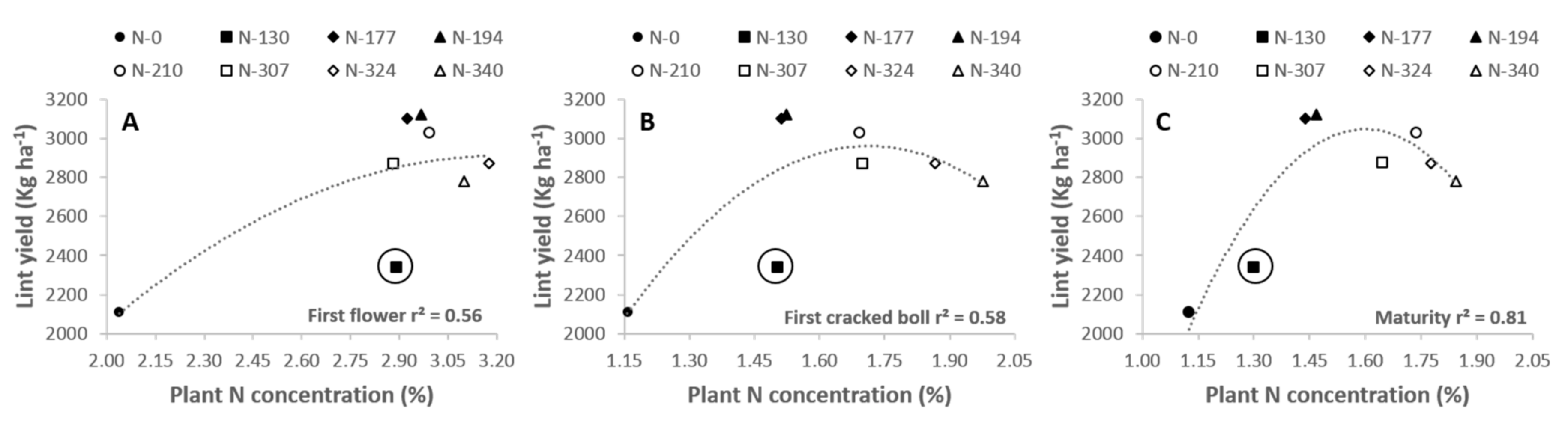
In agreement with other authors [15,16,17], a higher r2 was obtained for the relationships between the chlorophyll-sensitive indices (NDRE, SCCCI, TCARI/OSAVI and TGI) and lint yield later rather than earlier in the crop season (Figure 6). This was because less strong relationships between lint yield and plant N concentration were found at early stages of the crop than at maturity (Figure 9). However, it has to be noted that the treatment receiving all the fertilizer by means of an application of top-dressed Urea (N-130, highlighted in Figure 9 with a circle) on 10 December, impaired that relationship at first flower and around first cracked boll. In fact, the performance at predicting lint yield of the spectral indices sensitive to the chlorophyll content at the early stages of the crop (at 62 and 83 DAS), slightly improved in the case of the NDRE and TCARI/OSAVI and notably improved in the case of the SCCCI (r2 = 0.61 and 0.69 at 62 and 83 DAS) when the N-130 treatment was not taken into account (data not shown).
5. Conclusions
In this study, spectral measurements from an UAS enabled the assessment of the spatial and temporal variability of crop N status in a commercial cotton farm. The results show the challenges of using remote sensing in cotton to make fertilization recommendations at early stages of the crop.
At first flower, SCCCI was the index that best performed at detecting the variability in plant N% among treatments. The indices performance at distinguishing plant N status improved as the season progressed, when crop N demand increased and soil N availability became limiting in the treatments fertilized with zero N or the lowest N rate. Thus, around first cracked boll and maturity, the linear regression obtained for the relationships between the VIs and both plant N% and N uptake was statistically significant, with the highest r2 values obtained at maturity.
Based on these results, when using UAS to assess cotton variability in crop N status, we recommend monitoring SCCCI at early stages of the crop, from first flower to peak bloom, when the variability can be detected and fertilizer applications can still have an effect on lint yield. Moreover, we suggest the possibility of using NDRE measurements at maturity as a potential tool to identify areas with higher or lower defoliant application needs to make prescriptive applications in order to increase harvest efficiency. Nevertheless, further definition of relationships for this purpose are required.
SCCCI, TCARI/OSAVI and NDRE were the indices that best predicted lint yield early in the crop season (83 DAS). Results obtained from this study showed that at early stages of the crop, when cotton N demand is low and soil N availability may be enough to meet the plant N requirements, other factors may also influence plant growth and, therefore, challenge the use of structure-sensitive spectral indices such as the NDVI for predicting lint yield. The visible band index VARI performed similarly to the NDVI at predicting yield across the season, pointing out this index as an interesting option for yield prediction in cotton when only low-cost visible-band digital cameras are available.
Acknowledgments
The authors thank the great co-operation provided by the Stott family and staff at Stott Farms. The Cotton Research and Development Corporation (CRDC) and Deakin University funded the research.
Author Contributions
Carlos Ballester contributed to the field data acquisition, processing and analysis of the field and remote sensing data, and writing of the article. John Hornbuckle contributed to the remote sensing data acquisition and methodology. James Brinkhoff assisted in the remote sensing data analysis and contributed to the writing of the paper. John Smith assisted in the experimental field supervision and field data acquisition. Wendy Quayle was responsible of the experimental field design and field data acquisition, contributed to the field data processing and analysis, and participated in the writing of the article. All the authors contributed to revise the article.
Conflicts of Interest
The authors declare no conflict of interest. The funding sponsors had no role in the design of the study; in the collection, analyses, or interpretation of data; in the writing of the manuscript, or in the decision to publish the results.
References
- Gerik, T.J.; Oosterhuis, D.M.; Torbert, H.A. Managing cotton nitrogen supply. Adv. Agron. 1998, 64, 115–147. [Google Scholar]
- World Fertilizer Trends and Outlook to 2018; FAO: Rome, Italy, 2015; p. 66.
- Ali, N. Review: Nitrogen utilization features in cotton crop. Am. J. Plant Sci. 2015, 6, 987–1002. [Google Scholar] [CrossRef]
- Good, A.G.; Beatty, P.H. Fertilizing nature: A tragedy of excess in the commons. PLoS Biol. 2011, 9, e1001124. [Google Scholar] [CrossRef] [PubMed]
- Snyder, C.S.; Davidson, E.A.; Smith, P.; Venterea, R.T. Agriculture: Sustainable crop and animal production to help mitigate nitrous oxide emissions. Curr. Opin. Environ. Sustain. 2014, 9–10, 46–54. [Google Scholar] [CrossRef]
- Cottoninfo. Cottoninfo on-Farm Nitrogen Trials and N-Use Practices. Available online: https://www.cottoninfo.com.au/publications/cottoninfo-nitrogen-trials-report (accessed on 8 November 2017).
- Zhou, G.; Yin, X. Assessing nitrogen nutritional status, biomass and yield of cotton with ndvi, spad and petiole sap nitrate concentration. Exp. Agric. 2017, 1–18. [Google Scholar] [CrossRef]
- Mulla, D.J. Twenty five years of remote sensing in precision agriculture: Key advances and remaining knowledge gaps. Biosyst. Eng. 2013, 114, 358–371. [Google Scholar] [CrossRef]
- Buscaglia, H.J.; Varco, J.J. Early detection of cotton leaf nitrogen status using leaf reflectance. J. Plant Nutr. 2002, 25, 2067. [Google Scholar] [CrossRef]
- Tarpley, L.; Reddy, K.R.; Sassenrath-Cole, G.F. Reflectance indices with precision and accuracy in predicting cotton leaf nitrogen concentration. Crop Sci. 2000, 40, 1814–1819. [Google Scholar] [CrossRef]
- Read, J.J.; Tarpley, L.; McKinion, J.M.; Reddy, K.R. Narrow-waveband reflectance ratios for remote estimation of nitrogen status in cotton. J. Environ. Qual. 2002, 31, 1442–1452. [Google Scholar] [CrossRef] [PubMed]
- Raper, T.B.; Varco, J.J. Canopy-scale wavelength and vegetative index sensitivities to cotton growth parameters and nitrogen status. Precis. Agric. 2015, 16, 62–76. [Google Scholar] [CrossRef]
- Yang, C.; Bradford, J.M.; Wiegand, C.L. Airborne multispectral imagery for mapping variable growing conditions and yields of cotton, grain sorghum, and corn. Trans. ASAE 2001, 44, 1983–1994. [Google Scholar] [CrossRef]
- Raper, T.B.; Varco, J.J.; Hubbard, K.J. Canopy-based normalized difference vegetation index sensors for monitoring cotton nitrogen status. Agron. J. 2013, 105, 1345–1354. [Google Scholar] [CrossRef]
- Gutierrez, M.; Norton, R.; Thorp, K.R.; Wang, G. Association of spectral reflectance indices with plant growth and lint yield in upland cotton. Crop Sci. 2012, 52, 849–857. [Google Scholar] [CrossRef]
- Zarco-Tejada, P.J.; Ustin, S.L.; Whiting, M. Temporal and spatial relationships between within-field yield variability in cotton and high-spatial hyperspectral remote sensing imagery. Agron. J. 2005, 97, 641–653. [Google Scholar] [CrossRef]
- Zhao, D.; Reddy, K.R.; Kakani, V.G.; Read, J.J.; Koti, S. Canopy reflectance in cotton for growth assessment and lint yield prediction. Eur. J. Agron. 2007, 26, 335–344. [Google Scholar] [CrossRef]
- Zhang, C.; Kovacs, J.M. The application of small unmanned aerial systems for precision agriculture: A review. Precis. Agric. 2012, 13, 693–712. [Google Scholar] [CrossRef]
- Salamí, E.; Barrado, C.; Pastor, E. Uav flight experiments applied to the remote sensing of vegetated areas. Remote Sens. 2014, 6, 11051–11081. [Google Scholar] [CrossRef] [Green Version]
- Muharam, F.; Maas, S.; Bronson, K.; Delahunty, T. Estimating cotton nitrogen nutrition status using leaf greenness and ground cover information. Remote Sens. 2015, 7, 7007–7028. [Google Scholar] [CrossRef]
- Maresma, Á.; Ariza, M.; Martínez, E.; Lloveras, J.; Martínez-Casasnovas, J. Analysis of vegetation indices to determine nitrogen application and yield prediction in maize (zea mays l.) from a standard uav service. Remote Sens. 2016, 8, 973. [Google Scholar]
- Caturegli, L.; Corniglia, M.; Gaetani, M.; Grossi, N.; Magni, S.; Migliazzi, M.; Angelini, L.; Mazzoncini, M.; Silvestri, N.; Fontanelli, M.; et al. Unmanned aerial vehicle to estimate nitrogen status of turfgrasses. PLoS ONE 2016, 11, e0158268. [Google Scholar] [CrossRef] [PubMed]
- Hunt, E.R.; Horneck, D.A.; Spinelli, C.B.; Turner, R.W.; Bruce, A.E.; Gadler, D.J.; Brungardt, J.J.; Hamm, P.B. Monitoring nitrogen status of potatoes using small unmanned aerial vehicles. Precis. Agric. 2017, 1–20. [Google Scholar] [CrossRef]
- Zhu, J.; Wang, K.; Deng, J.; Harmon, T. Quantifying nitrogen status of rice using low altitude uav-mounted system and object-oriented segmentation methodology. In Proceedings of the ASME/IEEE International Conference on Mechatronic and Embedded Systems and Applications, San Diego, CA, USA, 30 August–2 September 2009; pp. 603–609. [Google Scholar]
- Isbell, R.F. The Australian Soil Classification; CSIRO: Collingwood, Australia, 2002; Volume 4. [Google Scholar]
- Grabham, M. Bankless Channel Irrigation Systems. In WATERpack—A Guide for Irrigation Management in Cotton and Grain Farming Systems, 3rd ed.; Cotton Research and Development Corporation (CRDC): Narrabri, Australia, 2012; pp. 388–391. [Google Scholar]
- Hunt, E.R.; Doraiswamy, P.C.; McMurtrey, J.E.; Daughtry, C.S.T.; Perry, E.M.; Akhmedov, B. A visible band index for remote sensing leaf chlorophyll content at the canopy scale. Int. J. Appl. Earth Obs. GeoInf. 2013, 21, 103–112. [Google Scholar] [CrossRef]
- Gitelson, A.A.; Kaufman, Y.J.; Stark, R.; Rundquist, D. Novel algorithms for remote estimation of vegetation fraction. Remote Sens. Environ. 2002, 80, 76–87. [Google Scholar] [CrossRef]
- Rouse, J.W.; Haas, R.H.; Schell, J.A.; Deering, D.W. Monitoring Vegetation Systems in the Great Plains with ERTS. In Proceedings of the Third Earth Resources Technology Satellite-1 Symposium, Washington, DC, USA, 10–14 December 1973; Freden, S.C., Mercanti, E.P., Becker, M.A., Eds.; NASA: Washington, DC, USA, 1974; pp. 309–317. [Google Scholar]
- Gitelson, A.A.; Merzlyak, M.N. Remote estimation of chlorophyll content in higher plant leaves. Int. J. Remote Sens. 1997, 18, 2691–2697. [Google Scholar] [CrossRef]
- Haboudane, D.; Miller, J.R.; Tremblay, N.; Zarco-Tejada, P.J.; Dextraze, L. Integration of hyperspectral vegetation indices for prediction of crop chlorophyll content for application to precision agriculture. Remote Sens. Environ. 2002, 81, 416–426. [Google Scholar] [CrossRef]
- Li, F.; Miao, Y.; Hennig, S.D.; Gnyp, M.L.; Chen, X.; Jia, L.; Bareth, G. Evaluating hyperspectral vegetation indices for estimating nitrogen concentration of winter wheat at different growth stages. Precis. Agric. 2010, 11, 335–357. [Google Scholar] [CrossRef]
- Yu, K.; Leufen, G.; Hunsche, M.; Noga, G.; Chen, X.; Bareth, G. Investigation of leaf diseases and estimation of chlorophyll concentration in seven barley varieties using fluorescence and hyperspectral indices. Remote Sens. 2014, 6, 64–86. [Google Scholar] [CrossRef]
- Yu, K.; Li, F.; Gnyp, M.L.; Miao, Y.; Bareth, G.; Chen, X. Remotely detecting canopy nitrogen concentration and uptake of paddy rice in the northeast china plain. ISPRS J. Photogramm. Remote Sens. 2013, 78, 102–115. [Google Scholar] [CrossRef]
- Yang, C.; Greenberg, S.M.; Everitt, J.H.; Fernandez, C.J. Assessing cotton defoliation, regrowth control and root rot infection using remote sensing technology. Int. J. Agric. Biol. Eng. 2011, 4, 1–11. [Google Scholar]
- Rochester, I.J. Nutrient uptake and export from an australian cotton field. Nutr. Cycl. Agroecosyst. 2007, 77, 213–223. [Google Scholar] [CrossRef]
Figure 1.
Location of the commercial cotton farm where the study was conducted in Whitton, NSW, Australia.
Figure 1.
Location of the commercial cotton farm where the study was conducted in Whitton, NSW, Australia.
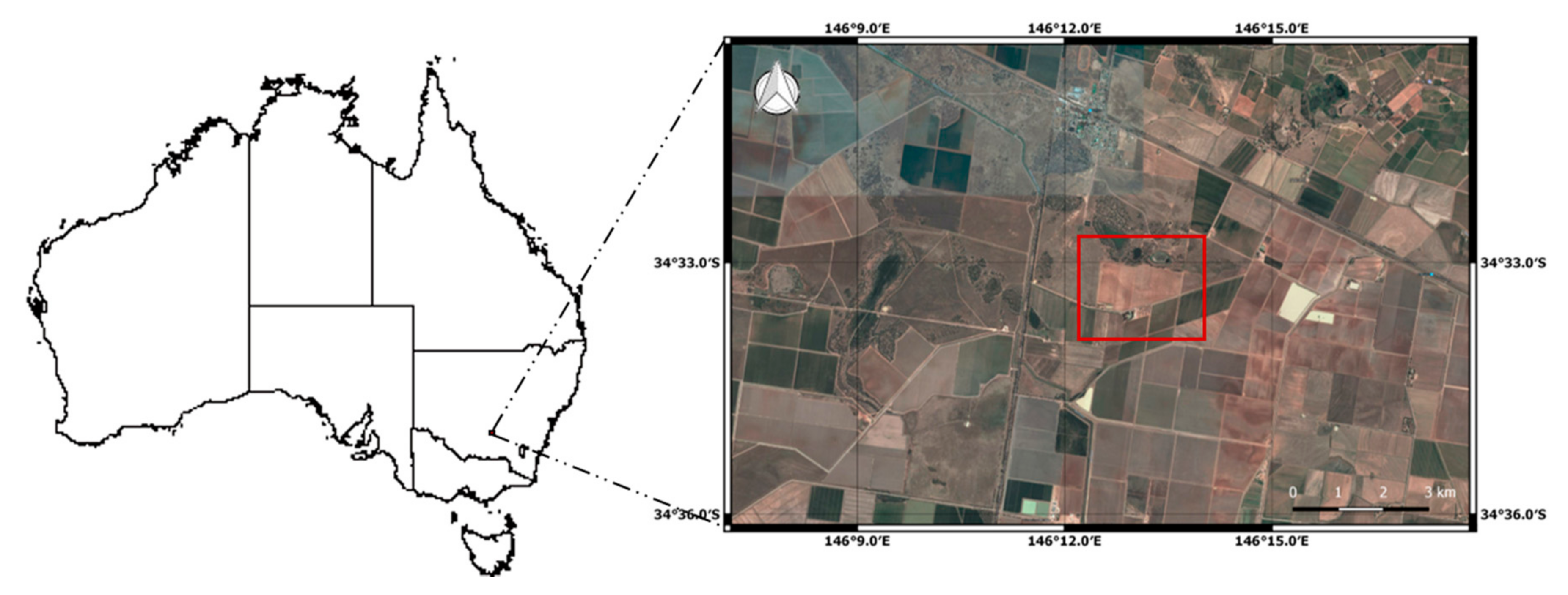
Figure 2.
Normalized difference red edge (NDRE) map for the fourth measurement date, 9 February 2016 (118 days after sowing), showing the distribution of the eight N rate treatments across the paddock and the masks used to extract the spectral information in each replicate.
Figure 2.
Normalized difference red edge (NDRE) map for the fourth measurement date, 9 February 2016 (118 days after sowing), showing the distribution of the eight N rate treatments across the paddock and the masks used to extract the spectral information in each replicate.
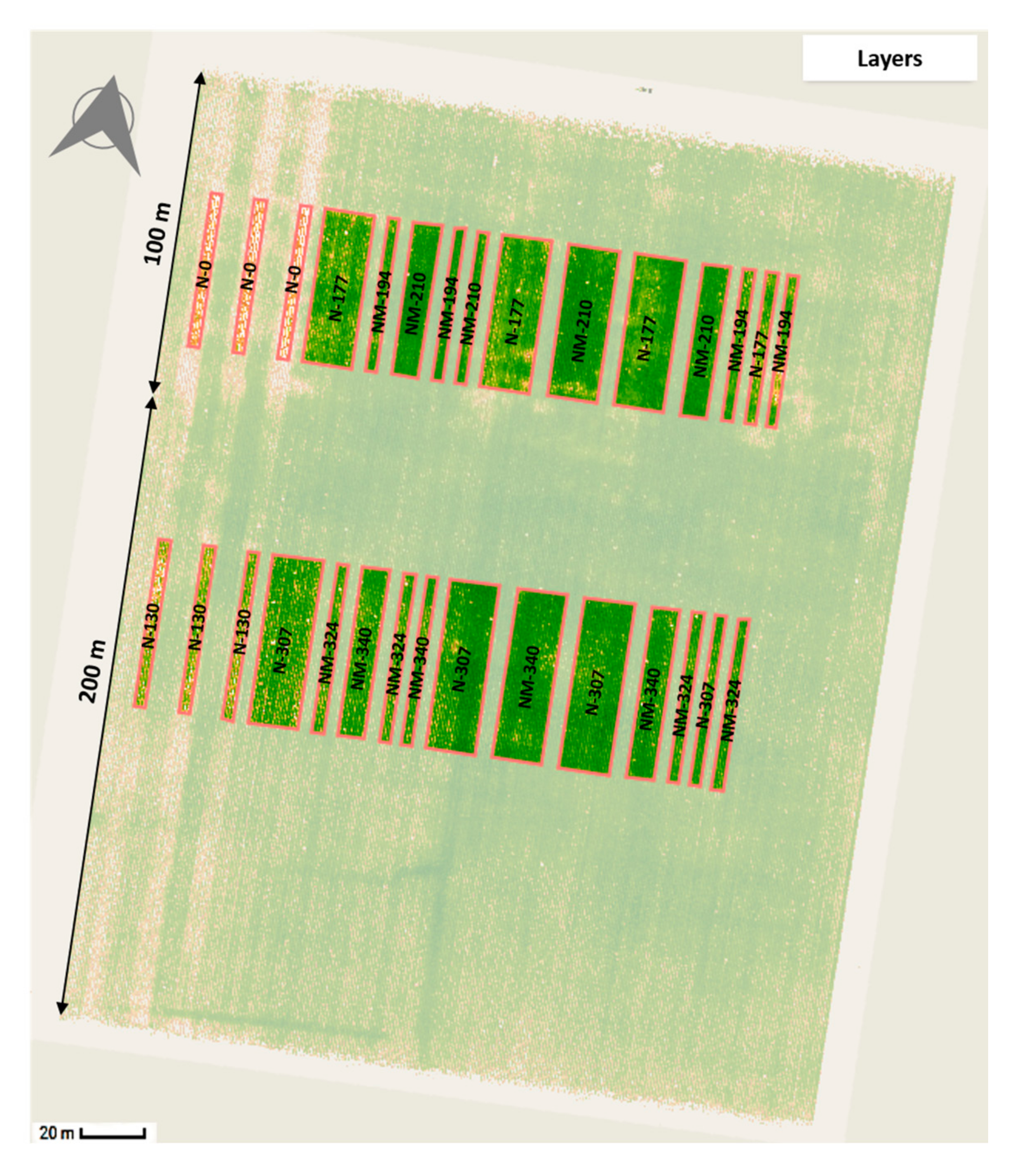
Figure 3.
Seasonal evolution of the normalized difference vegetation index (NDVI; A), normalized difference red edge index, NDRE (B), simplified canopy chlorophyll content index (SCCCI; C), transformed chlorophyll absorption reflectance index normalized by the optimized soil adjusted vegetation index (TCARI/OSAVI; D), triangular greenness index (TGI; E) and visible atmospherically resistant index (VARI; F) for all the fertilization treatments applied in the study.
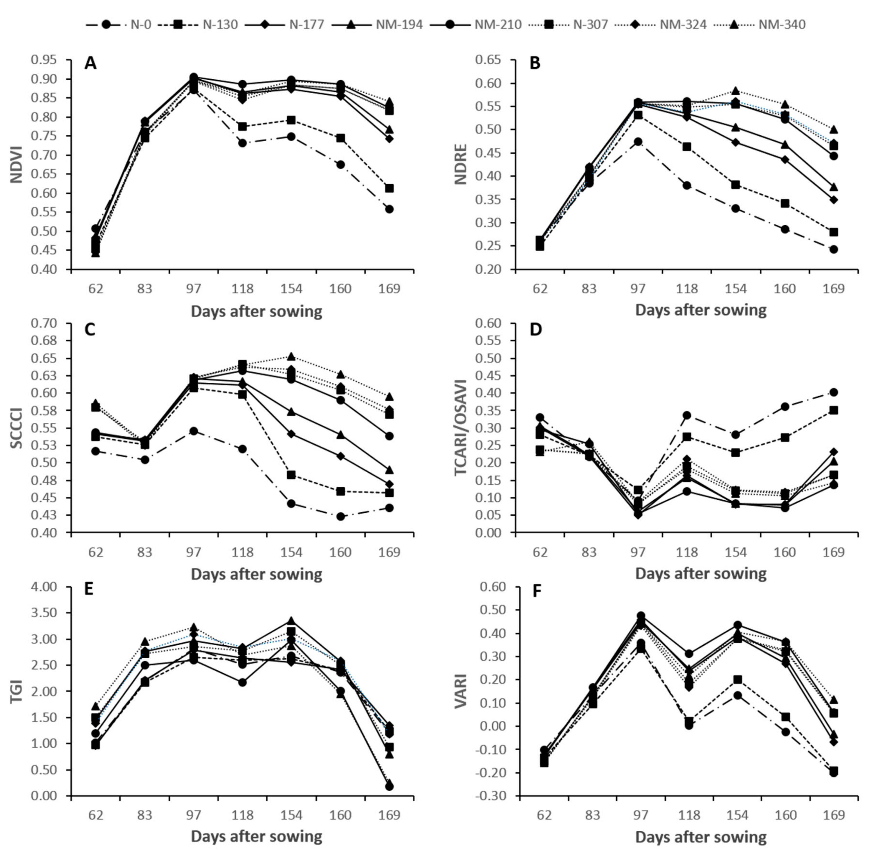
Figure 4.
Relationships between plant nitrogen concentration (N%) and the normalized difference vegetation index (NDVI; A), normalized difference red edge index, NDRE (B), simplified canopy chlorophyll content index (SCCCI; C), transformed chlorophyll absorption reflectance index normalized by the optimized soil adjusted vegetation index (TCARI/OSAVI; D), triangular greenness index (TGI; E) and visible atmospherically resistant index (VARI; F) at first flower, first cracked boll and maturity.
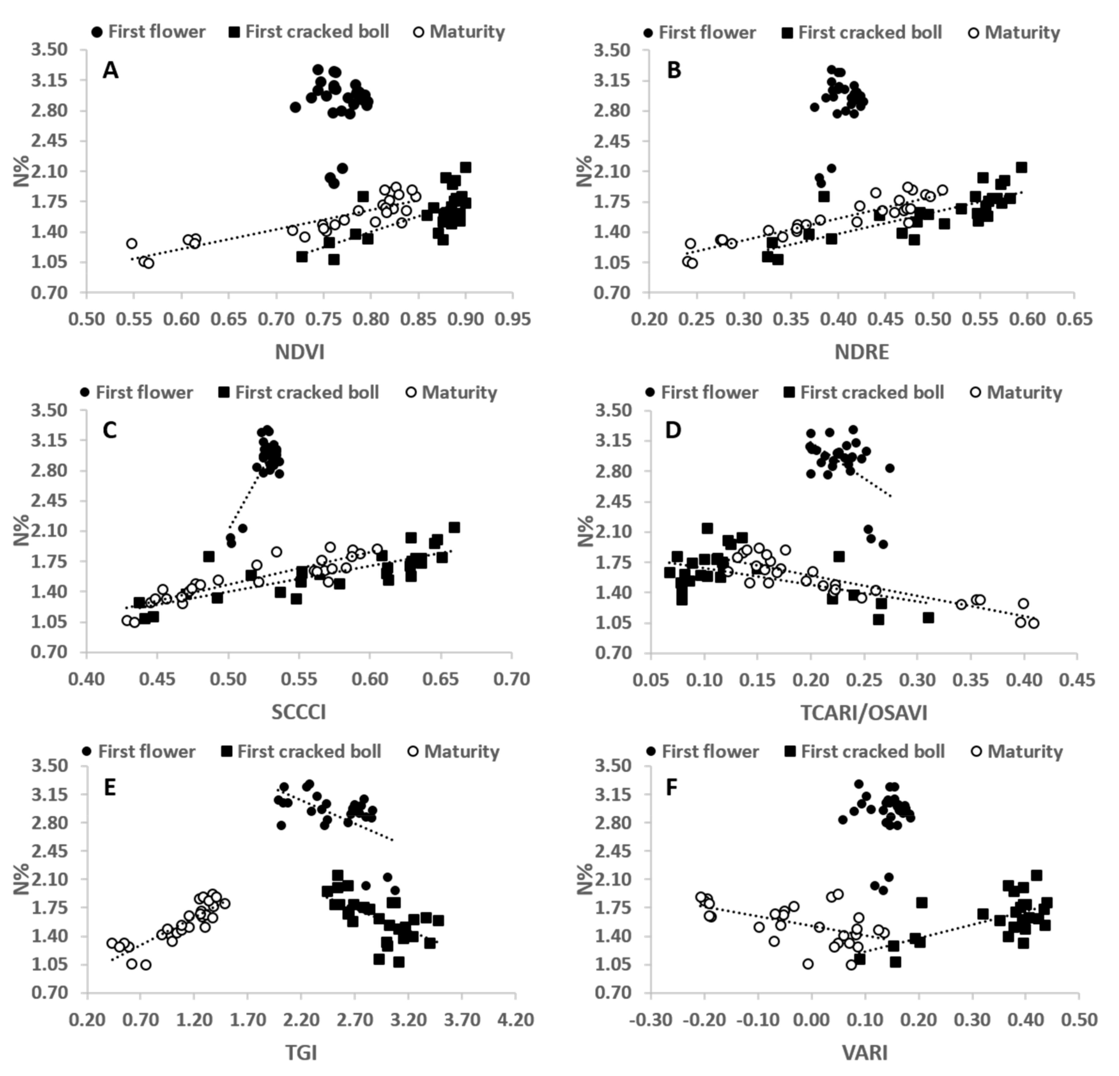
Figure 5.
Relationships obtained between nitrogen uptake (N uptake) and the normalized difference vegetation index (NDVI; A), normalized difference red edge index, NDRE (B), simplified canopy chlorophyll content index (SCCCI; C), transformed chlorophyll absorption reflectance index normalized by the optimized soil adjusted vegetation index (TCARI/OSAVI; D), triangular greenness index (TGI; E) and visible atmospherically resistant index (VARI; F) at first flower, first cracked boll and maturity.
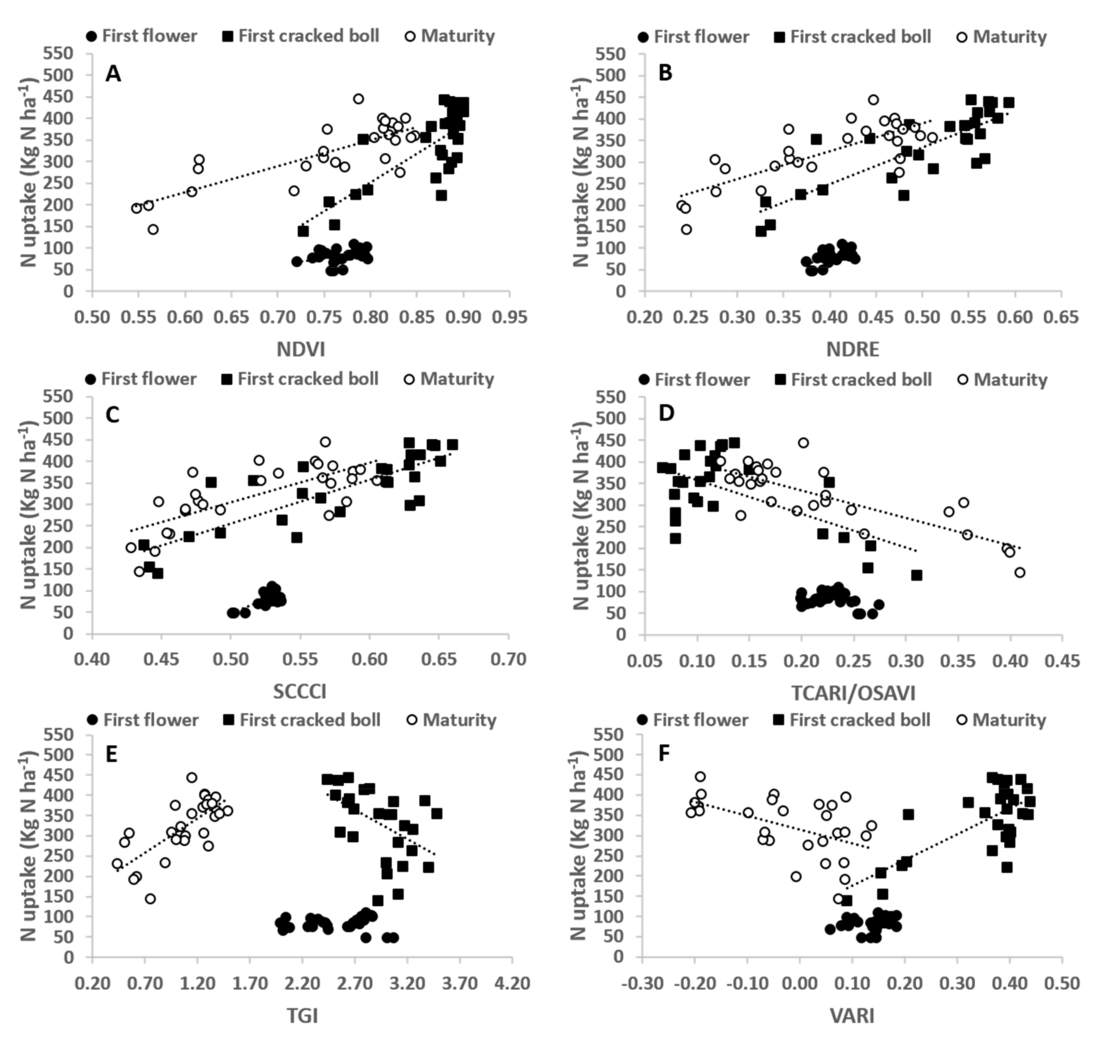
Figure 6.
Time series for the coefficient of determination obtained from the relationships between lint yield and the normalized difference vegetation index (NDVI; A), normalized difference red edge index, NDRE (B), simplified canopy chlorophyll content index (SCCCI; C), transformed chlorophyll absorption reflectance index normalized by the optimized soil adjusted vegetation index (TCARI/OSAVI; D), triangular greenness index (TGI; E) and visible atmospherically resistant index (VARI; F) using a linear and quadratic regression model.

Figure 7.
Relationships between N uptake and plant nitrogen concentration (N%) and crop dry mass at first flower (A,B, respectively), first cracked boll (C,D) and maturity (E,F).
Figure 7.
Relationships between N uptake and plant nitrogen concentration (N%) and crop dry mass at first flower (A,B, respectively), first cracked boll (C,D) and maturity (E,F).
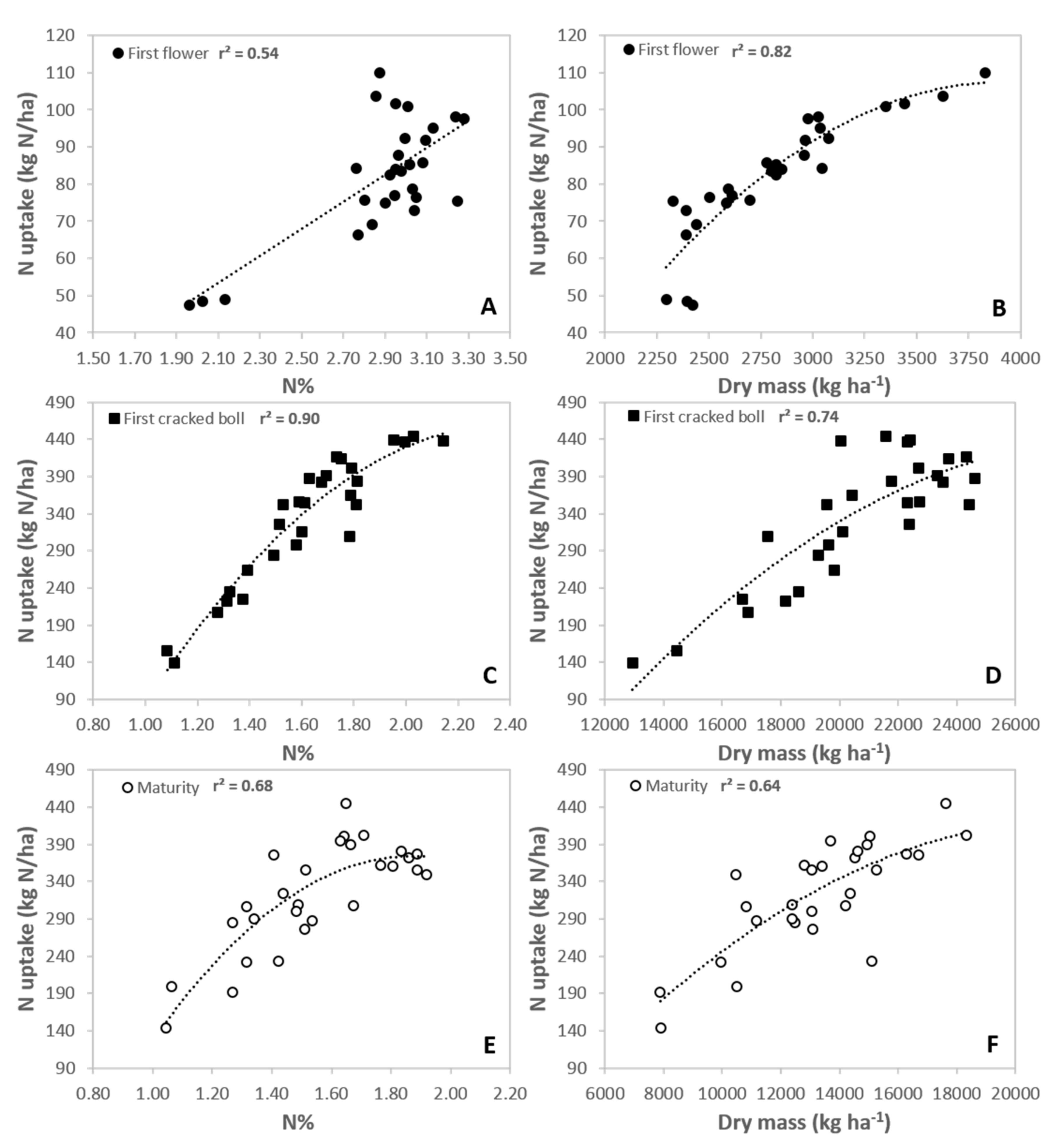
Figure 8.
Plant height measured in mid-December (left) and the relationship obtained between NDVI and plant height at 62 days after sowing (right).
Figure 8.
Plant height measured in mid-December (left) and the relationship obtained between NDVI and plant height at 62 days after sowing (right).
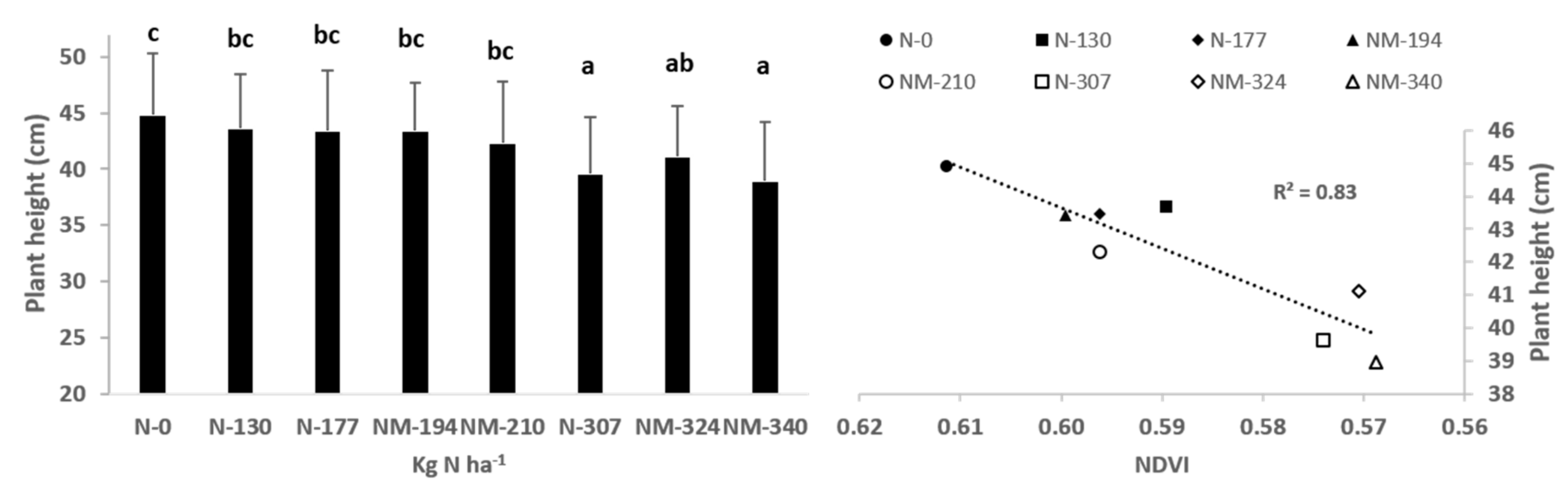
Figure 9.
Relationships between lint yield and plant N concentration at first flower (A), first cracked boll (B) and maturity (C). The treatment that received all nitrogen on 10 December 2015 by top dressing with Urea, N-130, is highlighted with a circle.
Figure 9.
Relationships between lint yield and plant N concentration at first flower (A), first cracked boll (B) and maturity (C). The treatment that received all nitrogen on 10 December 2015 by top dressing with Urea, N-130, is highlighted with a circle.


Table 1.
Total nitrogen (N) applied to each treatment and contribution and date of application of the four fertilizer products used in the study: poultry manure, diammonium phosphate (DAP), anhydrous ammonia (NH3-N) and urea. The number of replicates used for each treatment is also indicated.
Table 1.
Total nitrogen (N) applied to each treatment and contribution and date of application of the four fertilizer products used in the study: poultry manure, diammonium phosphate (DAP), anhydrous ammonia (NH3-N) and urea. The number of replicates used for each treatment is also indicated.
| Treatment | DAP * | NH3-N * | Poultry Manure * | Urea y | Total N Applied (kg ha−1) | Replicates |
|---|---|---|---|---|---|---|
| N-0 | 0 | 0 | 0 | 0 | 0 | 3 |
| N-130 | 0 | 0 | 0 | 130 | 130 | 3 |
| N-177 | 27 | 150 | 0 | 0 | 177 | 4 |
| NM-194 | 27 | 150 | 16.6 | 0 | 194 | 4 |
| NM-210 | 27 | 150 | 33.2 | 0 | 210 | 4 |
| N-307 | 27 | 150 | 0 | 130 | 307 | 4 |
| NM-324 | 27 | 150 | 16.6 | 130 | 324 | 4 |
| NM-340 | 27 | 150 | 33.2 | 130 | 340 | 4 |
* 23 September 2015; y 10 December 2015.
Table 2.
Vegetation indices computed from the spectral reflectance collected with the unmanned aerial system (UAS). The band centres used in this study for computing the spectral indices were 475, 560, 668, 717 and 840 nm for the blue, (B), green (G), red (R), red-edge (RE) and near infrared (NIR) bands, respectively.
| Vegetation Index | Formulation | Reference |
|---|---|---|
| NDVI | (NIR − R)/(NIR + R) | [29] |
| NDRE | (NIR − RE)/(NIR + RE) | [30] |
| SCCCI | NDRE/NDVI | [12] |
| TCARI/OSAVI | [3[(RE − R) − 0.2 (RE/G) (RE/R)]]/[(1 + 0.16) (NIR − R)/(NIR + R + 0.16)] RE/R | [31] |
| TGI | −0.5[(668 − 475)(R − G) − (668 − 560)(R − B)] | [27] |
| VARI | (G − R)/(G + R − B) | [28] |
Table 3.
Mean plant (above-ground part of the plant including bolls) nitrogen concentration (N%), nitrogen uptake (N uptake, kg N ha−1) and dry mass (DM, t ha−1) for each fertilization treatment at first flower, first cracked boll and maturity. Average lint yield (t ha−1) obtained at harvest is also shown.
| Treatment | First Flower (83 DAS *) | First Cracked Boll (154 DAS *) | Maturity (169 DAS *) | Lint Yield | ||||||
|---|---|---|---|---|---|---|---|---|---|---|
| N% | N Uptake | DM | N% | N Uptake | DM | N% | N Uptake | DM | ||
| N-0 | 2.04 ± 0.09 a | 48.3 ± 0.8 a | 2.4 ± 0.1 a | 1.16 ± 0.10 a | 167.0 ± 35.6 a | 14.7 ± 1.9 a | 1.13 ± 0.12 a | 178.3 ± 30.1 a | 8.7 ± 1.5 a | 2.11 ± 0.13 a |
| N-130 | 2.89 ± 0.12 b | 74.5 ± 4.8 b | 2.6 ± 0.1 ab | 1.50 ± 0.27 ab | 270.5 ± 71.0 ab | 18.3 ± 1.5 ab | 1.30 ± 0.03 ab | 273.9 ± 38.3 ab | 11.1 ± 1.3 ab | 2.34 ± 0.15 ab |
| N-177 | 2.93 ± 0.07 bc | 97.3 ± 11.8 d | 3.3 ± 0.5 c | 1.51 ± 0.14 ab | 322.8 ± 71.4 bc | 21.9 ± 2.8 b | 1.44 ± 0.04 bc | 310.3 ± 59.0 bc | 14.6 ± 1.7 bc | 3.10 ± 0.22 c |
| NM-194 | 2.97 ± 0.09 bc | 83.3 ± 6.9 cd | 2.8 ± 0.2 abc | 1.52 ± 0.10 ab | 304.4 ± 39.8 bc | 20.3 ± 1.3 b | 1.47 ± 0.09 bc | 308.1 ± 32.0 bc | 13.0 ± 1.7 abc | 3.12 ± 0.11 c |
| NM-210 | 2.99 ± 0.04 bc | 95.9 ± 9.2 cd | 3.2 ± 0.3 bc | 1.72 ± 0.19 bc | 384.2 ± 57.8 bc | 23.5 ± 1.7 b | 1.77 ± 0.11 d | 386.6 ± 19.4 c | 15.6 ± 2.0 c | 3.03 ± 0.07 c |
| N-307 | 2.88 ± 0.14 b | 75.1 ± 7.5 bc | 2.6 ± 0.3 abc | 1.70 ± 0.09 bc | 350.8 ± 56.5 bc | 21.1 ± 3.0 b | 1.65 ± 0.10 cd | 367.9 ± 70.6 bc | 14.6 ± 2.2 bc | 2.87 ± 0.06 c |
| NM-324 | 3.17 ± 0.10 c | 91.8 ± 10.4 bcd | 2.9 ± 0.3 abc | 1.87 ± 0.15 bc | 409.9 ± 38.2 c | 21.9 ± 1.2 b | 1.78 ± 0.15 d | 357.0 ± 38.1 bc | 13.7 ± 2.4 bc | 2.87 ± 0.20 c |
| NM-340 | 3.09 ± 0.14 bc | 83.0 ± 6.6 bcd | 2.7 ± 0.3 ab | 2.02 ± 0.17 c | 428.6 ± 19.8 c | 21.7 ± 1.4 b | 1.83 ± 0.04 d | 364.5 ± 12.4 bc | 13.6 ± 0.7 bc | 2.78 ± 0.26 bc |
Different letters between treatments within columns denote statistically significant differences at p < 0.05; * Days after sowing.
Table 4.
Coefficient of determination (r2) for the relationships obtained between mean nitrogen uptake (N uptake, kg N ha−1) and above-ground plant N concentration (N%) with the normalized difference vegetation index (NDVI), the normalized difference red edge index, NDRE, the simplified canopy chlorophyll content index (SCCCI), the transformed chlorophyll absorption reflectance index normalized by the optimized soil adjusted vegetation index (TCARI/OSAVI), the triangular greenness index (TGI) and visible atmospherically resistant index (VARI) at first flower (FF), first cracked boll (FCB) and maturity.
| Cotton Growth Stage | N% | N Uptake | ||||||||||
|---|---|---|---|---|---|---|---|---|---|---|---|---|
| NDVI | NDRE | SCCCI | TCARI/OSAVI | TGI | VARI | NDVI | NDRE | SCCCI | TCARI/OSAVI | TGI | VARI | |
| FF | 0.00 | 0.14 | 0.61 *** | 0.26 ** | 0.33 ** | 0.00 | 0.11 | 0.30 ** | 0.47 *** | 0.12 | 0.01 | 0.06 |
| FCB | 0.47 *** | 0.62 *** | 0.65 *** | 0.25 ** | 0.37 *** | 0.40 *** | 0.58 *** | 0.67 *** | 0.68 *** | 0.38 *** | 0.25 ** | 0.52 *** |
| Maturity | 0.77 *** | 0.84 *** | 0.80 *** | 0.76 *** | 0.74 *** | 0.29 ** | 0.65 *** | 0.62 *** | 0.53 *** | 0.65 *** | 0.51 *** | 0.26 ** |
** and *** denote statistical significance at p < 0.01 and 0.001, respectively.
© 2017 by the authors. Licensee MDPI, Basel, Switzerland. This article is an open access article distributed under the terms and conditions of the Creative Commons Attribution (CC BY) license (http://creativecommons.org/licenses/by/4.0/).
Share and Cite
MDPI and ACS Style
Ballester, C.; Hornbuckle, J.; Brinkhoff, J.; Smith, J.; Quayle, W. Assessment of In-Season Cotton Nitrogen Status and Lint Yield Prediction from Unmanned Aerial System Imagery. Remote Sens. 2017, 9, 1149. https://doi.org/10.3390/rs9111149
AMA Style
Ballester C, Hornbuckle J, Brinkhoff J, Smith J, Quayle W. Assessment of In-Season Cotton Nitrogen Status and Lint Yield Prediction from Unmanned Aerial System Imagery. Remote Sensing. 2017; 9(11):1149. https://doi.org/10.3390/rs9111149
Chicago/Turabian StyleBallester, Carlos, John Hornbuckle, James Brinkhoff, John Smith, and Wendy Quayle. 2017. "Assessment of In-Season Cotton Nitrogen Status and Lint Yield Prediction from Unmanned Aerial System Imagery" Remote Sensing 9, no. 11: 1149. https://doi.org/10.3390/rs9111149
Note that from the first issue of 2016, this journal uses article numbers instead of page numbers. See further details here.