Fusion Approaches for Land Cover Map Production Using High Resolution Image Time Series without Reference Data of the Corresponding Period


1
CESBIO (Centre d’Etudes Spatiales de la BIOsphere), Université de Toulouse, CNES/CNRS/IRD/UPS, 18 avenue Edouard Belin, 31401 Toulouse CEDEX 9, France
2
CNES (Centre National d’Etudes Spatiales), 18 avenue Edouard Belin, 31401 Toulouse CEDEX 9, France
*
Author to whom correspondence should be addressed.
Remote Sens. 2017, 9(11), 1151; https://doi.org/10.3390/rs9111151
Submission received: 10 October 2017
/
Revised: 30 October 2017
/
Accepted: 7 November 2017
/
Published: 9 November 2017
Abstract
:Optical sensor time series images allow one to produce land cover maps at a large scale. The supervised classification algorithms have been shown to be the best to produce maps automatically with good accuracy. The main drawback of these methods is the need for reference data, the collection of which can introduce important production delays. Therefore, the maps are often available too late for some applications. Domain adaptation methods seem to be efficient for using past data for land cover map production. According to this idea, the main goal of this study is to propose several simple past data fusion schemes to override the current land cover map production delays. A single classifier approach and three voting rules are considered to produce maps without reference data of the corresponding period. These four approaches reach an overall accuracy of around 80% with a 17-class nomenclature using Formosat-2 image time series. A study of the impact of the number of past periods used is also done. It shows that the overall accuracy increases with the number of periods used. The proposed methods require at least two or three previous years to be used.

1. Introduction
Land cover maps provide key information in many environmental and scientific applications. They can be used to monitor deforestation [1] or urban pressure [2] over croplands, for instance. Satellite imagery and, by extension, satellite image time series allow one to produce accurate land cover maps. In the past few years, the number of space-borne optical sensors has increased, making a wealth of useful data available for land use monitoring. The Landsat sensors provide useful data for land cover monitoring, especially Landsat 5 and 8, which are used to produce accurate land cover maps [3]. The Sentinel-2 system (S2), a pair of twin satellites dedicated to continental surface monitoring, is already providing high quality data for land cover maps. The first results obtained by using single date S2 images are promising [4], and by using S2 image time series, the performance should increase.
Supervised classification algorithms are the state of the art approach to producing land cover maps automatically [5]. Among these, the Support Vector Machine (SVM) and the Random Forest (RF) classifiers are the most widely used. These methods require, nevertheless, a large amount of reference data, that is samples for which the land cover class is known. This requirement is the main cause of the delay needed to produce a map. Indeed, the reference data can be provided by different sources. Field surveys to collect in situ data are tedious and expensive. On the other hand, the use of topographical databases is possible, but these data are available usually several years after the collection date. Generally, the delay depends on the source of reference data and also on the size of the mapped area.
Despite these delays, reference data comprise precious information that is gathered together over the years. In standard supervised classification, the reference data are seldom used for labeling samples, as they are valid only for the period (reference year, for instance) corresponding to their acquisition, because the landscape changes over time. However, considering reference data over the years allows one to know the landscape history. Therefore, training a classifier using imagery of the current period and reference data of a previous period can lead to low quality land cover maps. In the case of annual land cover map production, one uses images of the current year to produce a land cover map, but the reference data may have been collected more than one year earlier.
One could consider training a classifier with imagery corresponding to the period of the reference data and then apply the trained classifier to the imagery of the current period. Unfortunately, due to climate conditions (temperature, precipitations), cloud cover and other factors, the image time series of two different years can have different temporal patterns leading again to bad classification accuracy.
Some solutions to correct this kind of distortion in the data have been proposed in the literature: the Domain Adaptation (DA) techniques. In these approaches, the source domain is defined as known, i.e., corresponding reference data are available, and the target domain as unknown. The aim is to reduce the shift between the data or tuning the classifier parameters to use reference data of the source domain in the target domain. The state of the art DA methods are presented in Section 1.1, but they need some adaptations to be applied to the problem at hand. In the particular case addressed in this paper, each previous period with reference data must be considered as a source domain. In this work, instead of adapting DA techniques, we take a more pragmatic yet efficient approach in order to exploit several previous periods for the production of land cover maps without reference data for the current period. To this end, simple fusion schemes are proposed. Two studies are done in this paper, one regarding the performance of the fusion methods with a high number of previous periods and a second one to evaluate the sensitivity to the number of periods used.
The remainder of the paper is organized as follows: a short state of the art of DA methods is done in Section 1.1; the materials and methods used are presented in Section 2.1 and Section 2.3, respectively; finally, results are presented in Section 3 and discussed in Section 4 before conclusions are drawn in Section 5.
1.1. Short Review of Domain Adaptation Methods
As introduced in the previous section, the use of data from previous periods for the classification of data of the current period is addressed in this paper. This problem can be reduced to a distortion correction between past and current periods’ image time series. In the literature, the methods allowing one to correct important distortions between pairs of datasets are called Domain Adaptation (DA). The distorted datasets must be at least related.
In DA, a source domain is used to predict a target domain . For each domain, a probability is defined by and for and , respectively, where X is the input variable vector, i.e., the image time series described by spectral bands and derived indices, and Y is the output variable associated with a set of classes, i.e., the map nomenclature. is the domain where enough reference data are available, and has little or no reference data. The goal of a DA method is to adapt a classifier trained using data or the data directly to predict the samples.
A DA survey has recently been done by Tuia et al. [6]. In this survey, the authors present the most widely-used DA methods in remote sensing. They define four categories of algorithms:
- Feature extraction by selecting invariant features
- Adapting data distributions
- Adapting classifiers with semi-supervised approaches
- Adaptation of the classifier by active learning
The invariant feature extraction category is composed of algorithms similar to those used in feature selection approaches, as for instance Principal Component Analysis (PCA) to reduce the data dimensionality by keeping the most relevant features. In DA, the aim is to determine the features that suffer the least from the distortion between the two domains, by determining a projection matrix. With the set of invariant features, the distortion can be estimated, and a common space can be created. In this space, the and the extracted features are jointly used, as one domain. Therefore, this common space is stable, and it is possible to use the same classifier on both domains. In the literature, there are some works that present different invariant feature selection methods, for instance [7,8], where the authors use several distance measures to select the features.
This approach is mostly used to correct two kinds of distortions between the source and the target domains. The first is the variations of the illumination or the sensor angle of view. In our case, the image time series used are acquired with constant viewing angles and are radiometrically corrected and expressed in surface reflectance, which makes them invariant with respect to these issues. The second use case is when only a small part of the image is labeled and the target domain is another area of the same image. In our case, this problem is not considered, as a split of the area of interest into eco-climatic areas allows one to achieve good performance [9]. In an eco-climatic area, the classes’ time profiles are more homogeneous than in an entire image. In addition, a drawback of feature extraction in our case is that the increasing number of source domains requires the invariant features to be the same for each source domain. If the distortions between the different source domains are too important, a loss of discriminative information can occur, and therefore, a classifier loses generalization.
The second category of approaches deals with data distribution adaptation. As the first category of algorithms, this approach aims to adapt the data. The main difference is that the methods keep the original features and try to create a new space where the shift between and is reduced. In this new space, the two domains will be treated equally. A first approach considered in the literature is the use of a kernel matrix to project one domain into the other. There are many methods for matrix estimation [10,11]. A second approach aims to align the data distribution. These methods use histogram matching methods [12] or distance methods, such as Dynamic Time Warping (DTW) [13].
The main drawback of this approach, in our case, is that the data dimensionality will increase for each new source domain, leading to huge transformation matrices and statistical estimation issues. In the case of alignment methods, like DTW, for instance, the processing time will increase greatly since the process must be carried out between each source and target domain. In addition, the most efficient methods use the target domain labeled samples, which are not available in our case.
The two previous categories are used as a pre-processing step allowing one to use standard classifiers to predict the samples of the target domain. There are drawbacks shared by these two approaches in our application case, since they often use similarity, covariance, the dependence measure or minimization functions. Their efficiency depends on the data dimension, which can highly increase if many previous periods are used. In the literature, sometimes, feature extraction is used before applying the data distribution algorithm to improve the performance [8].
The third category of approaches uses semi-supervised algorithms. For these methods, it is mandatory that the features and the nomenclature are the same in both domains. A classifier is defined as semi-supervised when target domain data are used to change the decision rules of a supervised classifier trained on the source domain. For instance, in the work of Bruzzone et al. [14], a classifier is trained on the source domain, and the sample distributions of the target domain are used to tune the parameters of the classifier. Another approach is to use a cascade classifier [15], more often using radial basis function neural networks, which include target domain samples in the learning step.
The main drawback of this approach, in our case, is that the training of a semi-supervised classifier is often an iterative process. At each iteration, target domain samples are added to the training sample set. This training could be long, and it is mandatory to train the classifier again when a new period is considered. The main difficulty of this approach is the target domain samples’ selection, by similarity or clustering, which will have a direct impact on the classifier performance. The naive solution to this sample selection problem requires user interaction.
The last category is active learning. This approach also aims at adapting the classifier. It can be considered as a particular case of the semi-supervised approach where the target domain samples’ selection is done by the user. Often, the target domain samples are labeled by hand, by visual interpretation (this is the meaning of “active”). As the sample selection quickly becomes time consuming and the learning becomes costly, the samples must be well-chosen. An active learning algorithm ends when the user is satisfied with the results. Many active learning algorithms exist in the literature, but as they are not automated, they are not considered in this work.
The interested reader is invited to refer to the survey [6] for more information. In addition, a most complete survey was done by Patel et al. [16], considering all DA methods used in machine learning, with applications to computer vision.
Looking at the particular case addressed in this paper, none of these algorithms seem to be appropriate. Indeed, they do not take advantage of several previous periods to predict the current one. In this particular case, each previous period must be considered as a source domain, and the target domain is the current period image time series. That means that it is necessary to process the domain adaptation for each pair of past and current periods. This will be very costly in terms of processing time and complexity of use. As a consequence, the existing DA methods will not be considered here, but this work should be a first step to adapting existing DA methods to a multi-source domain problem. In this paper, the usefulness of multiple source domains will be shown. To this end, several fusion schemes, used in some DA works as a post-processing task, are proposed to avoid the costly domain adaptation process.
2. Materials and Methods
2.1. Optical Data
To study the contribution of previous periods to produce land cover maps, a large number of periods is required. To this end, 8 years of Formosat-2 images are available for the same area, near Toulouse in the southwest of France, shown in Figure 1. Formosat-2 has the advantage of a high resolution of 8 m and a high revisit cycle of one day, over a 24 km × 24 km area. In comparison to the sensors used mostly at the moment for land cover mapping, Landsat 8 has a 30-m resolution and a revisit cycle of 16 days. Sentinel-2 when fully operational will provide 10-m resolution images every 5 days.
The Formosat-2 images are processed with MACCS (Multi-sensor Atmospheric Correction and Cloud Screening) [17] to correct atmospheric effects and provide cloud, cloud shadow and saturation masks. Formosat-2 has 4 spectral bands (blue, red, green and NIR) to which two spectral indices, the Normalized Difference Vegetation Index (NDVI) and the brightness, are added as image features. The time series is the concatenation of spectral reflectances, NDVI and brightness [3].
As the number of usable images varies over the periods, mainly due to cloud cover, a temporal interpolation is performed. To this end, a regular time grid is defined, with a time gap of 14 days. This interpolation does not induce a loss of accuracy [3] and allows one to have the same temporal sampling for every period. The time grid begins 1 October of the previous year and ends 31 December of the current year. This time slicing corresponds to the phenology cycle and the agricultural season in the study area. Therefore, at the end of these pre-processing steps, 7 time series (from 2007 to 2013) with identical dates for every period are available.
2.2. Reference Data
The reference data used in this work were obtained by field surveys. These surveys were done every year, so for each time series, corresponding reference data are available. The reference data are randomly split into two independent datasets, where 50% of the samples of each class are used for training and 50% for validation. This split was done 10 times for each period in order to compute average performance over several runs of the experiments, as well as confidence intervals.
The reference data are composed of the 17 classes shown in Table 1. This set of classes includes winter (wheat, barley, …) and summer (maize, sunflower, …) crop classes, natural classes (water, forest, …) and artificial surfaces. As is possible to see in Table 1, the number of samples available for each class varies greatly. We therefore have a stratified sample, but not exactly proportional to the distribution of classes in the entire study area, although ranks are preserved. Indeed, the field campaign represents only a small part of the study area as shown in Figure 1. We can see majority classes that are represented by a large number of samples such as “wheat” and “broad-leaved tree” and also minority classes with very few samples like “wasteland” or “barley”. This wide nomenclature is not restricted to any specific application, and therefore, conclusions for general land cover mapping may be drawn from the results.
2.3. Methodology
Supervised classification algorithms outperform other approaches for land cover mapping using satellite image time series. Random Forests (RF) [18] achieve very good performance for these tasks [9], whose general workflow can be described as follows:
- Data pre-processing
- Classifier training using labeled data to define the decision rules
- Classification, using a trained classifier to predict the classes of unlabeled data
- Post-processing
In the ideal case, reference data would be available for the current period and a good quality land cover map could be obtained. This ideal case (called standard supervised in the following) will be used in the experiments as an upper bound for the performance. At the other end, using a classifier trained using images and reference data from a previous period will produce a lower quality land cover map since, as explained above, the image time series for the current period may be different from the ones from the period used for the training. We will also use this naive case to define the lower bound of the classification performance.
The fusion approaches presented in this work aim at increasing the quality of the maps from the naive case towards the ideal standard supervised case.
In this section, the global workflow is presented first, and then, the different methods used are detailed. Finally, the validation procedure is explained.
2.3.1. Global Approach
The data preparation is described in Section 2.1, and it is the same for all the methods. The training step, shown in Figure 2, requires an image time series and reference data to learn the decision rules. The dedicated set of reference data is used. The generated output model contains the decision rules. The learning step can be repeated as many times as different datasets are available. For each pair of image time series and reference data, a classifier can be trained, using the samples of the training set. Each sample has the same number of features defined by the time series (see Section 2.1). In our case, each previous period yields a classifier. Another possibility is to use together several previous periods for training a single classifier. In this case, the number of training set samples is where p is the number of previous periods considered, and is the same for each period (see Section 2.1). In both cases, the procedure is the same: a training set is built using image time series pixels and their corresponding labels, and this training set is used to train a classifier.
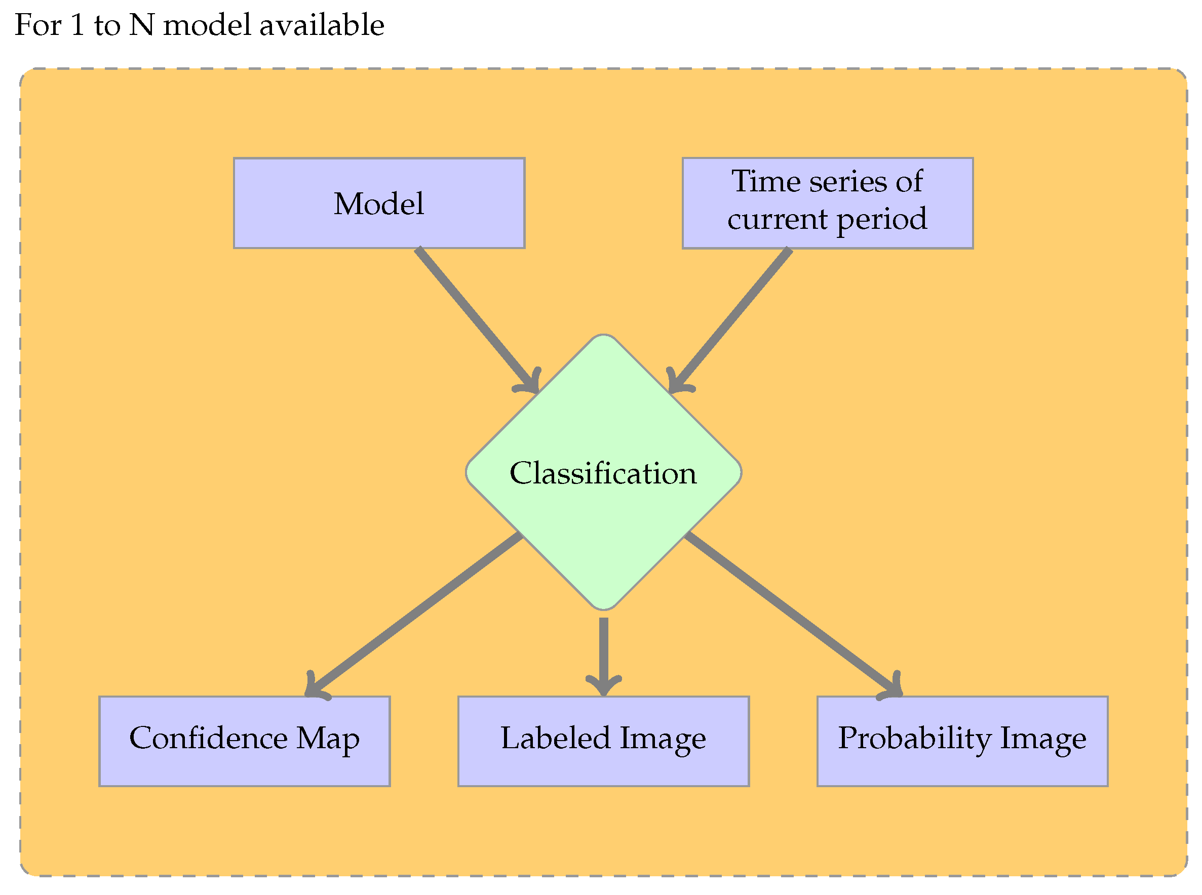
The next step is the classification shown in Figure 3. This step requires a classifier trained in Step 1 and one time series as the input. The classifier predicts the labels of the time series and also gives access to the number of trees that voted for each label. When converted to proportions, these values can be interpreted as probabilities for each class. The probability of the majority class is called confidence. In the standard supervised case, the time series used is the same for the training and the classification steps. All the available classifiers can be used to classify the image time series of the current period, producing land cover maps, confidence values and probabilities for each class. These will later be used in fusion approaches to derive the final land cover map.
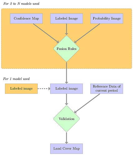
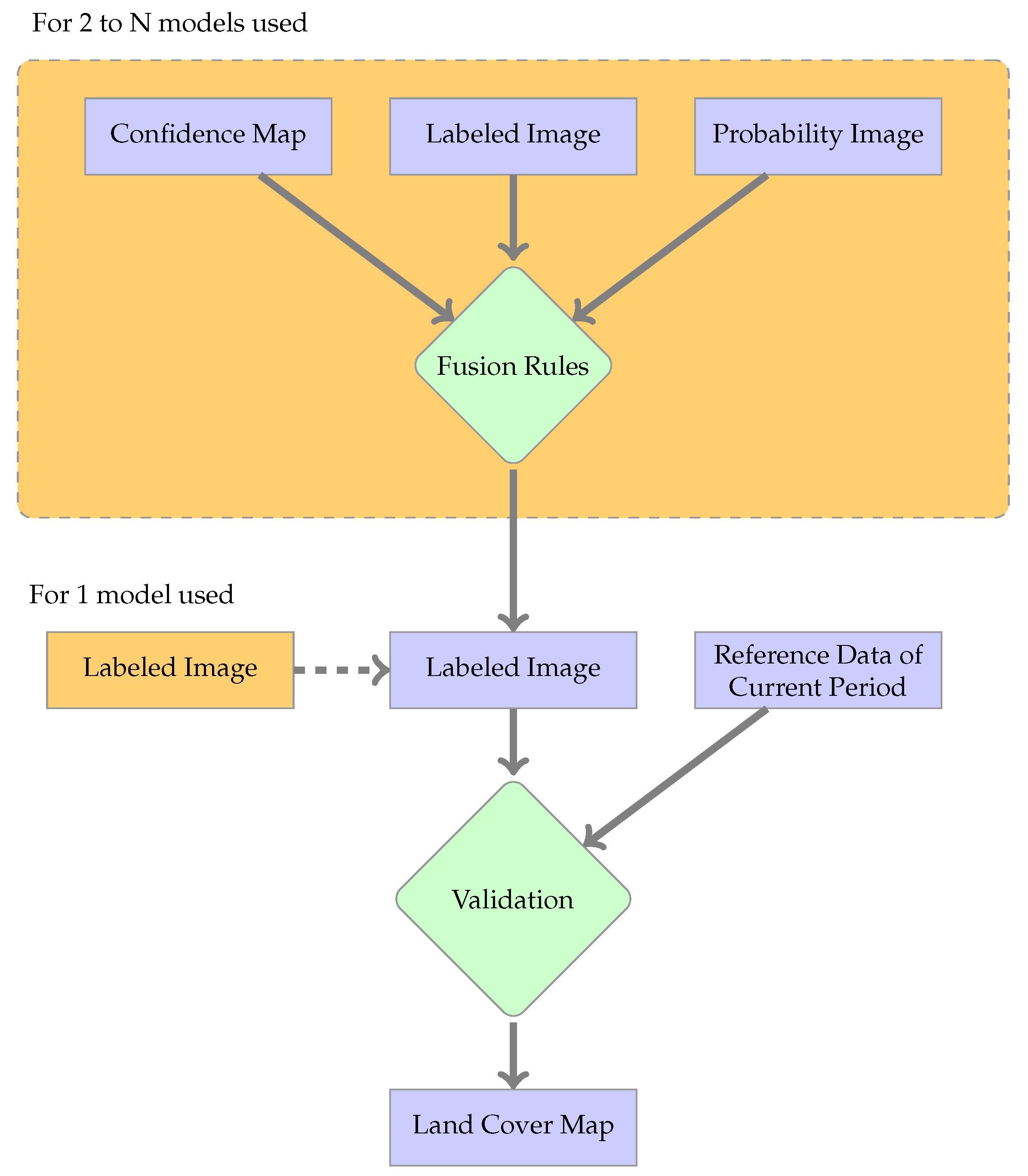
The last step is post-processing, shown in Figure 4. This step regroups different optional tasks. For the standard supervised classification, the validation of the labeled image is the only task. If several classifiers are used, fusion processing is mandatory to produce a unique land cover map.
This workflow allows one to generate a land cover map from an image time series. More specific cases of use are explained in the following part of this section.
2.3.2. Fusion Methods
Two main fusion approaches are considered in this work.
The first approach is based on the work of Flamary et al. [19]. In their work, the authors use several previous periods to train different classifiers. The best results are obtained by training a unique classifier with all previous periods. In our work, a single RF is trained, using a training set with samples. To this end, all the available pairs of time series and reference data are used for training. The aim is to feed the classifier with all the variability present in previous periods so that no particular period is favored.
The second approach uses the fusion of land cover maps. Every previous period (i.e., a set of samples for a given period p) is used to train a classifier, and then, each classifier is applied to the current period image time series. The fusions of the produced maps are performed in a post-processing step using voting. Three voting methods are proposed:
- Majority Voting (MV): Each map votes for a label, and the majority label is chosen. In the case of a tie, a non-decision label is chosen.
- Confidence Voting (CV): Each voter selects a class, and the confidence is used as a weight to compute a score per label. The label with the highest score is chosen. This approach considers only the labels chosen by the classifier.
- Probability Voting (PV): Each voter uses the probability values to give a weight to every possible label. The label with the highest score is chosen.
Since the causality (the temporal order of the periods) is not used, in order to increase the amount of data available, it is possible to produce the land cover map for period N fusing classifiers trained with data of periods and , where n represents other periods. Therefore, each of the 7 years of the dataset will be considered as the current period and the other 6 as the previous periods.
This study is split into two parts. The first one uses all the available periods to evaluate the performance of each method. In the second part, the impact of the history size (the number of previous periods) is evaluated. For this part, each period is again considered as the current period, and the history is created by using all the combinations of 2, 3, …, up to 6 periods.
2.4. Validation Procedure
The land cover maps produced with each approach are validated using standard metrics. A confusion matrix [20], where the rows are predicted labels and the columns the reference labels, is computed using the validation sets. In this matrix, the diagonal elements represent the number of correctly classified pixels, and the rest of the matrix is misclassification. The Overall Accuracy (OA) is the sum of the diagonal elements divided by the sum of all elements of the confusion matrix. For each class, the F1-score (Fscore) is considered, which is the harmonic mean of precision and recall.
- The recall (also called producer’s accuracy) is computed for each class. To this end, in the confusion matrix, each row is considered (one per class), and the number of correctly classified pixels is divided by the total number of reference data pixels of that class.
- The precision (also called user’s accuracy) is computed considering the column of the confusion matrix. It is the fraction of correctly classified pixels with regard to all pixels classified as this class.
As vote methods are considered, a particular label is used for non-decision. It is used when there is a tie in a vote. In addition, this label must not be included in metrics computation [21], as this label does not represent an error in the classification. Therefore, it will be necessary to study the ratio of non-decided pixels in the vote output to temper the metrics values.
3. Results
In this section, the results obtained with the different methods are presented. This section is organized as follows: first, the performances of the two baselines are analyzed, then the four fusion methods are compared, and finally, the analysis of the impact of the history size on the performance is done.
3.1. Baseline Configuration Analysis
The baseline configurations are defined by the use of a classifier trained with the image time series of one period, which is then applied to the same period (standard supervised case) or to another period (naive baseline). Table 2 presents the OA obtained for all these combinations of periods. In this table, the rows represent the period of the data used to train the classifier and the columns the period of the image time series used to produce the map, i.e., the current period. Each value is the average of the 10 runs (different draws of training and validation samples), and the 90% confidence intervals are shown. The diagonal represents the standard supervised case.
As expected, the standard supervised OA is very good with narrow confidence intervals and similar values for all the available years. In contrast, the naive baseline yields lower performance, and in most of the cases, OA is below 70% with large disparities between the different cases. The OA gap between the standard supervised and the naive baselines is larger than 20%, and therefore, there is room for improvement.
It is interesting to analyze the variability of the performance of a given classifier when applied to different periods. For instance, the classifier trained with the 2012 image time series yields an OA of 74% when applied to the 2010 image time series, but it can produce maps with OA as low as 51% for other period. This means that changing the input time series for a given classifier does not have the same impact on the predictions as changing the decision rules, i.e., the classifier trained on a given time series to predict a new time series. As shown in the table, the performance for a given time series (column), except for the standard supervised case, is rather stable. This effect is due in part to the robustness of RF to the noise present in the labeled data [22]. The robustness of RF is also shown by the very narrow confidence intervals.
In the following sections, the naive baselines will be summarized as the average values of the columns of Table 2 removing the diagonal.
3.2. Results of the Fusion Strategies
Two metrics are used for the evaluation: the OA for a global evaluation and the Fscore of each class. The OAs obtained by the two baselines and the four fusion methods are plotted in Figure 5. The x-axis is the year of the image time series used for producing the maps, and the y-axis corresponds to OA values. Confidence intervals are also plotted for each method. Solid lines are the baselines, and dashed lines represent the fusion methods. The Sup curve is the average OA obtained by the standard Supervised baseline. The NBM (Naive Baseline Mean) curve is the OA average values of the Naive Baseline, and each point in the curve is the average of 60 values, i.e., the 10 runs of the sic available years. The NBMax curve is the best run of the naive case, i.e., one among 60 values. The SC curve shows the Single Classifier performance. MV, CV and PV are Majority Voting, Confidence Voting and Probability Voting, respectively.
Figure 5 shows that the four fusion methods and the naive baseline curves follow the same trends. This effect proves the contribution of history, which can provide an amount of useful information. Using this information year by year (naive baseline) is not efficient, but by combining all periods, the performance increases by around 20%. The three voting methods yield similar results, and their differences lay within the confidence intervals. The single classifier approach results are slightly above the other methods, which can be interpreted as fusing the history data before training the classifier yields better results than a post-classification fusion. However, the main drawback of the single classifier is that the training with all periods has to be performed again every time a new period is available. This is not the case for the other methods, for which only the training of the new available period has to be performed. The standard supervised baseline is often 10% better than the fusion methods, but for the years 2010 and 2012, the single classifier performs better than the standard supervised case.
Table 3 shows the Fscore values obtained with the six methods. The average values are computed by using all the periods for each method. The aim of this table is to show the behavior of the methods for the different classes of the nomenclature in order to give further insight.
The values obtained by the standard Supervised case (Sup) are as expected. Indeed, the wide variations of Fscore values, as for broad-leaved tree at 93% and barley at 30%, are usual for the nomenclature considered: wheat and barley have very close temporal and spectral signatures, and barley being a minority class, it is often classified as wheat; the same issue happens with sorghum classified as maize.
Three categories of classes can be determined by looking at Fscore variations:
- Classes for which the Fscore is similar to the standard supervised case, with narrow confidence intervals. These classes are: broad-leaved tree, pine, wheat, maize and sunflower.
- Classes for which the Fscore is lower than for the standard supervised case and the confidence intervals are wide. These classes are: rapeseed, artificial surfaces, wasteland, river, lake, gravel pit and grass.
- Classes for which the Fscore is very low with narrow confidence intervals. These classes are: barley, sorghum, soybean, fallow lands and hemp.
This categorization represents a known situation, introduced in Section 2.2. Indeed, the first category of classes is usually well predicted for the study area, as they are representative of the land use of the region (majority classes). In contrast, the third category of classes is often confused by the classifiers with majority classes, as wheat and barley for instance. Other classes, such as hemp or soybean, are not representative of the crops in the studied region, so they are minority classes. This categorization could be used to show the nomenclature limits, i.e., the confusion done by the classifier whatever the reference dataset used. A possible extension of this categorization is to associate a weight to each category and to use this to reduce the imbalance between minority and majority class. Another extension could be to propose automatically, using these categories and logical rules, a fusion of the third category classes with the others classes: for instance, wheat and barley could be fused into a winter cereal class. This kind of class fusion should reduce confusion and therefore improve the performance.
3.3. Impact of the History Size
In this section, we study the impact of the history size (the number of previous periods) on the performance of the methods. For this experiment, seven periods are available; therefore, six periods can be combined to create the history dataset. For the particular case where only one period is available, only the naive approach is possible. The other methods need at least two periods of history data. Figure 6 shows the OA obtained as a function of the history size. The x-axis is the number of periods in the history, and the y-axis is the OA value. The OA of the standard supervised case (Sup) and naive case (NBM) are extracted from Table 2 and give the lower and upper bounds.
For the other history sizes, all possible combinations of periods are used, and the average is plotted. As one could have expected, performance increases with increasing history size. The two weighted voting methods provide similar results, and the disparity decreases when the number of periods increases. The single classifier is better than the other fusion methods, and the OA values increase faster than the ones of voting methods. With four periods of past data, the SC is able to provide a map with 80% accuracy. This accuracy is reached by the voting methods when six previous periods are used. The subset of previous period data used has a minor impact on the performance, as shown by the very narrow confidence intervals.
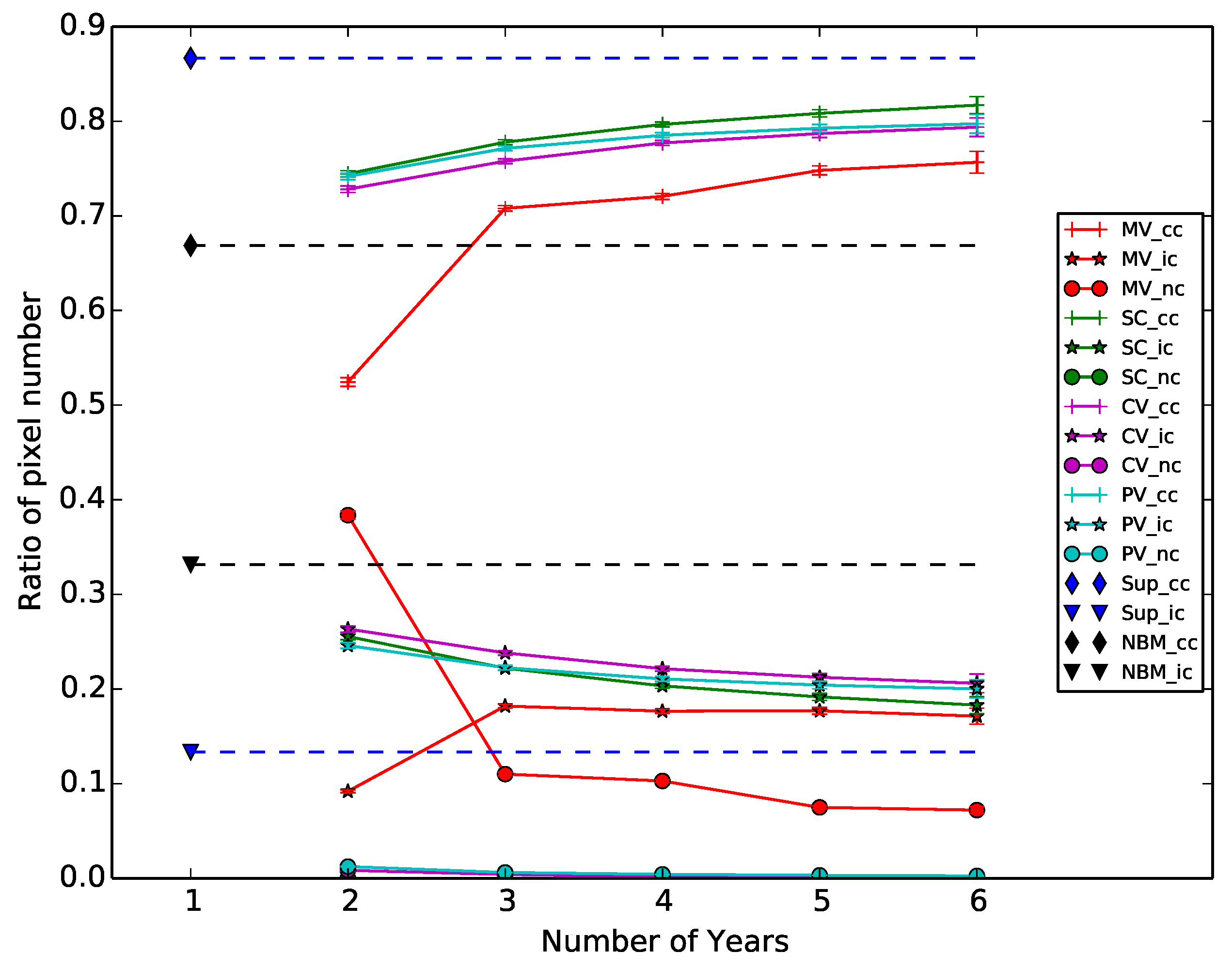
The majority voting approach has an unexpected behavior: when only two periods are used, the majority voting produces a map with 85% OA and decreases to 80% when three periods are used. This is due to the amount of undecided pixels, which are not taken into account for the OA computation. Figure 7 shows the ratio of correctly classified, incorrectly classified and undecided (not classified) pixels in the validation step. The x-axis represents the history size and the y-axis the ratio values. This figure shows that the two weighted voting approaches produce a small amount of undecided pixels, while the majority voting approach always produces over 10% of these pixels.
A high number of undecided pixels is a major drawback. Furthermore, the ratio of pixels is always between the limits defined by the baselines, except for the majority voting. Therefore, the single classifier seems to be the best method to produce a map with past data.
4. Discussion
The efficiency of the proposed methods is shown by comparing their performance to the baselines. The proposed fusion methods yield similar performance, and they are closer to the standard supervised case and much better than the naive baselines.
In addition, the OA trends in Figure 6 show the contribution of using different previous periods to produce the land cover map without reference to the corresponding period. The single classifier seems slightly better than the other methods, but it requires training the classifier again, using all past period, for every new period available. In contrast, the voting methods yield similar OA using previously trained classifiers, which is a great advantage in the case of large-scale land cover map production since the previous time series do not need to be available once the classifier has been trained. The proposed voting methods are simpler than the DA methods, as they only require a data pre-processing procedure, as explained in Section 2.1. Consequently, increasing the number of previous periods only impacts the processing time and not the algorithm complexity. Therefore, they are limited by the number of previous periods available as explained in the previous section. Another limit of these methods is related to the nomenclature as the minority classes are incorrectly predicted, as shown in the Fscore in Table 3. Errors in the reference data can also induce the confusion of the minority classes in voting methods. The majority voting produces many undecided pixels, which is a major drawback. However, the accuracy obtained is very high, which could be useful for some of the DA techniques of the literature based on semi-supervised or active learning, which require labeled samples in the target domain. The small amount of errors in this labeled image should reduce the number of training iterations. The labeled pixels by majority voting could also be used to reduce the amount of data in the projection matrix estimation or to align the data distributions, for instance. Another perspective would be using the history to evaluate the methods’ capability regarding the nomenclature using the Fscore variations and the confidence intervals, as presented in Section 3, and propose a new voting system.
The voting methods and the single classifier give very similar results. It is therefore interesting to give some insight in terms of algorithmic complexity. The classification complexity, , i.e., the application of the decision rules, is the same for each method. A first case to consider is the year the process begins. In the case of voting methods, it is necessary to train N classifiers with a cost proportional to the amount of input samples. The cost of training all required classifiers is therefore . In the case of the single classifier, the complexity is because the samples for all available periods are used. Hence, for the first year, the learning time is equivalent. For the single classifier, the cost of the whole procedure is finally . For the voting methods, it is necessary to carry out one classification per available period and also to perform the fusion operation, that is a complexity of , with the fusion complexity. In this case, the processing time for the voting methods is greater than the one required for the single classifier. The second case represents the following years. In this case, the models required for voting methods have already been computed. It is only necessary to train the classifier for the new available period. We therefore have a processing complexity of ; whereas in the case of the single classifier, it is necessary to carry out the complete training again by including the new period. Therefore, the complexity is . Since typically , voting methods are faster after the first year of processing. In addition, voting methods do not require keeping samples, but only trained classifiers. This represents an advantage in terms of storage.
5. Conclusions
In this paper, the use of images and reference data from previous periods to produce the current period land cover map without current reference data for standard supervised classification is addressed. This work is focused on showing the contribution of the use of multiple previous periods’ data instead of using only one as is usually done in the domain adaptation literature. It constitutes of a first step before adapting the DA methods to deal with multiple source domains. To this end, three voting methods are proposed, majority voting, and two weighted votes: confidence voting and probability voting. The results show similar Overall Accuracy (OA), ranging from 75% to 85%, depending on the datasets.
Another method is considered, a single classifier trained by using data from several previous periods. This approach yields slightly better results than the others. The second part of this work evaluated the impact on the performance of the number of available previous periods. As expected, when more periods are available, the performance increases. The single classifier is slightly better than the others as its performance increases faster when the history size increases. All these results are stable as proven by the very narrow confidence intervals. They are encouraging and prove the interest in using several previous periods’ data. The single classifier requires keeping all the samples’ image data available to train the decision rules again instead of the voting methods requiring only the previous trained classifiers. In the case of working at a very large scale, this can be a major drawback for the single classifier. Therefore, the voting methods represent a good alternative to DA methods for producing large-scale land cover maps without reference data of the same period.
Acknowledgments
This work is funded by the French spatial agency (CNES) and the region Occitanie, and it has been carried out at the CESBIO (Centre d’Etudes Spatiales de la BIOsphere) laboratory. The authors would like to thank their CESBIO colleagues for their help in data collection.
Author Contributions
Benjamin Tardy is the main author of this manuscript. He implemented the processing chain and processed the data. Jordi Inglada designed and participated in the analysis of the data. Julien Michel participated in the discussion during the system design and gave valuable methodological advice. All authors have been involved in the writing of the manuscript.
Conflicts of Interest
The authors declare no conflict of interest.
References
- Hansen, M.C.; Potapov, P.V.; Moore, R.; Hancher, M.; Turubanova, S.A.; Tyukavina, A.; Thau, D.; Stehman, S.V.; Goetz, S.J.; Loveland, T.R.; et al. High-Resolution Global Maps of 21st-Century Forest Cover Change. Science 2013, 342, 850–853. [Google Scholar] [CrossRef] [PubMed]
- Dewan, A.M.; Yamaguchi, Y. Land Use and Land Cover Change in Greater Dhaka, Bangladesh: Using Remote Sensing to Promote Sustainable Urbanization. Appl. Geogr. 2009, 29, 390–401. [Google Scholar] [CrossRef]
- Inglada, J.; Arias, M.; Tardy, B.; Hagolle, O.; Valero, S.; Morin, D.; Dedieu, G.; Sepulcre, G.; Bontemps, S.; Defourny, P.; et al. Assessment of an Operational System for Crop Type Map Production Using High Temporal and Spatial Resolution Satellite Optical Imagery. Remote Sens. 2015, 7, 12356–12379. [Google Scholar] [CrossRef]
- Immitzer, M.; Vuolo, F.; Atzberger, C. First Experience With Sentinel-2 Data for Crop and Tree Species Classifications in Central Europe. Remote Sens. 2016, 8, 166. [Google Scholar] [CrossRef]
- Srivastava, P.K.; Han, D.; Rico-Ramirez, M.A.; Bray, M.; Islam, T. Selection of Classification Techniques for Land Use/land Cover Change Investigation. Adv. Space Res. 2012, 50, 1250–1265. [Google Scholar] [CrossRef]
- Tuia, D.; Persello, C.; Bruzzone, L. Domain Adaptation for the Classification of Remote Sensing Data: An Overview of Recent Advances. IEEE Geosci. Remote Sens. Mag. 2016, 4, 41–57. [Google Scholar] [CrossRef]
- Bruzzone, L.; Persello, C. A Novel Approach To the Selection of Spatially Invariant Features for the Classification of Hyperspectral Images With Improved Generalization Capability. IEEE Trans. Geosci. Remote Sens. 2009, 47, 3180–3191. [Google Scholar] [CrossRef]
- Persello, C.; Bruzzone, L. Kernel-Based Domain-Invariant Feature Selection in Hyperspectral Images for Transfer Learning. IEEE Trans. Geosci. Remote Sens. 2016, 54, 2615–2626. [Google Scholar] [CrossRef]
- Inglada, J.; Vincent, A.; Arias, M.; Tardy, B.; Morin, D.; Rodes, I. Operational High Resolution Land Cover Map Production At the Country Scale Using Satellite Image Time Series. Remote Sens. 2017, 9, 95. [Google Scholar] [CrossRef]
- Matasci, G.; Volpi, M.; Kanevski, M.; Bruzzone, L.; Tuia, D. Semisupervised Transfer Component Analysis for Domain Adaptation in Remote Sensing Image Classification. IEEE Trans. Geosci. Remote Sens. 2015, 53, 3550–3564. [Google Scholar] [CrossRef]
- Bailly, A.; Chapel, L.; Tavenard, R.; Camps-Valls, G. Nonlinear Time-Series Adaptation for Land Cover Classification. IEEE Geosci. Remote Sens. Lett. 2017, 14, 1–5. [Google Scholar] [CrossRef]
- Inamdar, S.; Bovolo, F.; Bruzzone, L.; Chaudhuri, S. Multidimensional Probability Density Function Matching for Preprocessing of Multitemporal Remote Sensing Images. IEEE Trans. Geosci. Remote Sens. 2008, 46, 1243–1252. [Google Scholar] [CrossRef]
- Petitjean, F.; Inglada, J.; Gancarski, P. Satellite Image Time Series Analysis Under Time Warping. IEEE Trans. Geosci. Remote Sens. 2012, 50, 3081–3095. [Google Scholar] [CrossRef]
- Bruzzone, L.; Prieto, D. Unsupervised Retraining of a Maximum Likelihood Classifier for the Analysis of Multitemporal Remote Sensing Images. IEEE Trans. Geosci. Remote Sens. 2001, 39, 456–460. [Google Scholar] [CrossRef]
- Bruzzone, L.; Cossu, R. A Multiple-Cascade-Classifier System for a Robust and Partially Unsupervised Updating of Land-Cover Maps. IEEE Trans. Geosci. Remote Sens. 2002, 40, 1984–1996. [Google Scholar] [CrossRef]
- Patel, V.M.; Gopalan, R.; Li, R.; Chellappa, R. Visual Domain Adaptation: A Survey of Recent Advances. IEEE Signal Process. Mag. 2015, 32, 53–69. [Google Scholar] [CrossRef]
- Hagolle, O.; Huc, M.; Pascual, D.V.; Dedieu, G. A multi-temporal method for cloud detection, applied to FORMOSAT-2, VENμS, LANDSAT and SENTINEL-2 images. Remote Sens. Environ. 2010, 114, 1747–1755. [Google Scholar] [CrossRef] [Green Version]
- Breiman, L. Random Forest. Mach. Learn. 2001, 45, 5–32. [Google Scholar] [CrossRef]
- Flamary, R.; Fauvel, M.; Dalla Mura, M.; Valero, S. Analysis of Multitemporal Classification Techniques for Forecasting Image Time Series. IEEE Geosci. Remote Sens. Lett. 2015, 12, 953–957. [Google Scholar] [CrossRef]
- Congalton, R.G. A review of assessing the accuracy of classifications of remotely sensed data. Remote Sens. Environ. 1991, 37, 35–46. [Google Scholar] [CrossRef]
- Lam, L.; Suen, S. Application of Majority Voting To Pattern Recognition: An Analysis of Its Behavior and Performance. IEEE Trans. Syst. Man Cybern. Part A Syst. Hum. 1997, 27, 553–568. [Google Scholar] [CrossRef]
- Pelletier, C.; Valero, S.; Inglada, J.; Champion, N.; Sicre, C.M.; Dedieu, G. Effect of Training Class Label Noise on Classification Performances for Land Cover Mapping With Satellite Image Time Series. Remote Sens. 2017, 9, 173. [Google Scholar] [CrossRef]
Figure 1.
Formosat-2 image of the 6 May 2013 and the corresponding reference data from the field campaign.
Figure 1.
Formosat-2 image of the 6 May 2013 and the corresponding reference data from the field campaign.
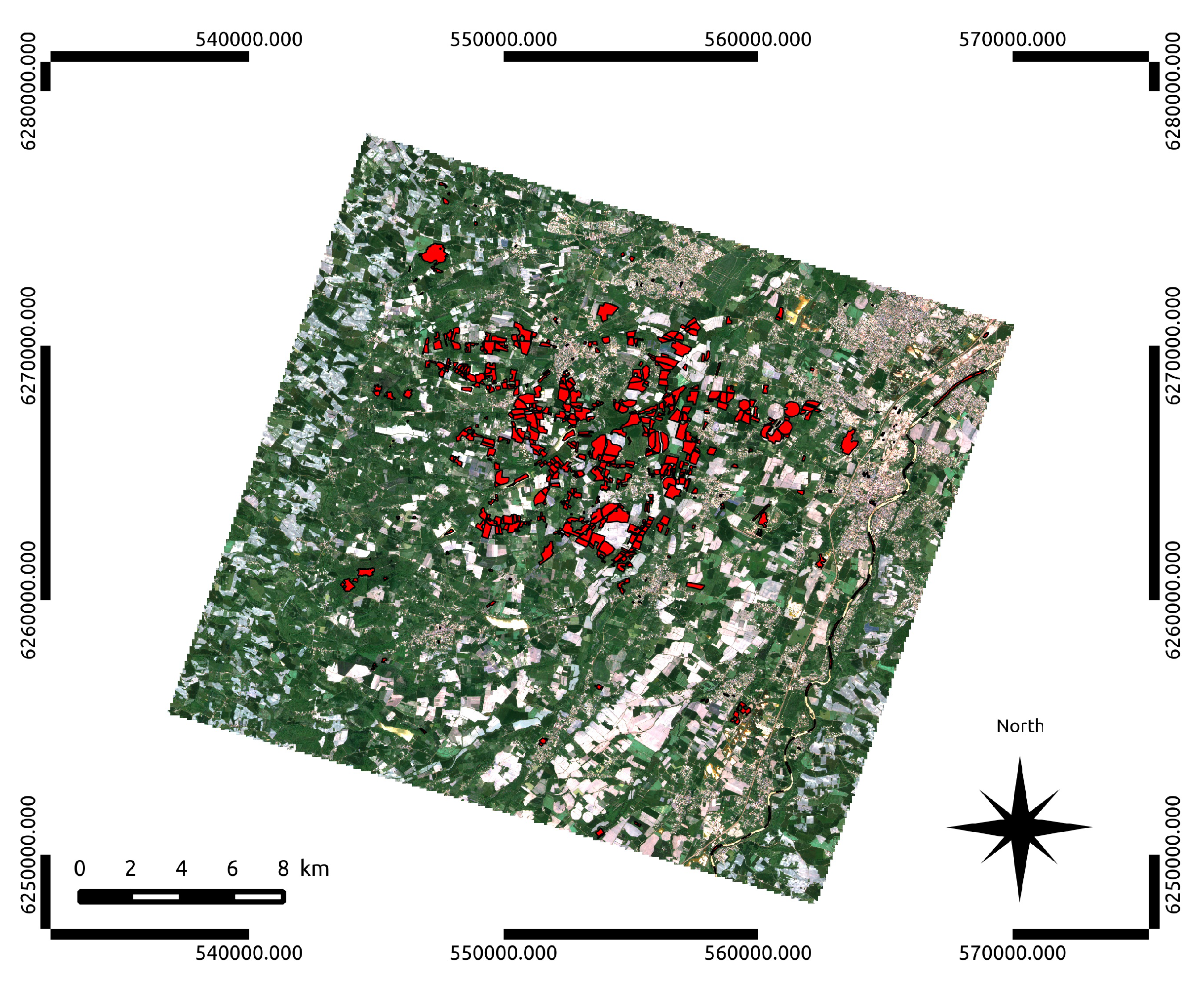
Figure 2.
Workflow of the learning step.
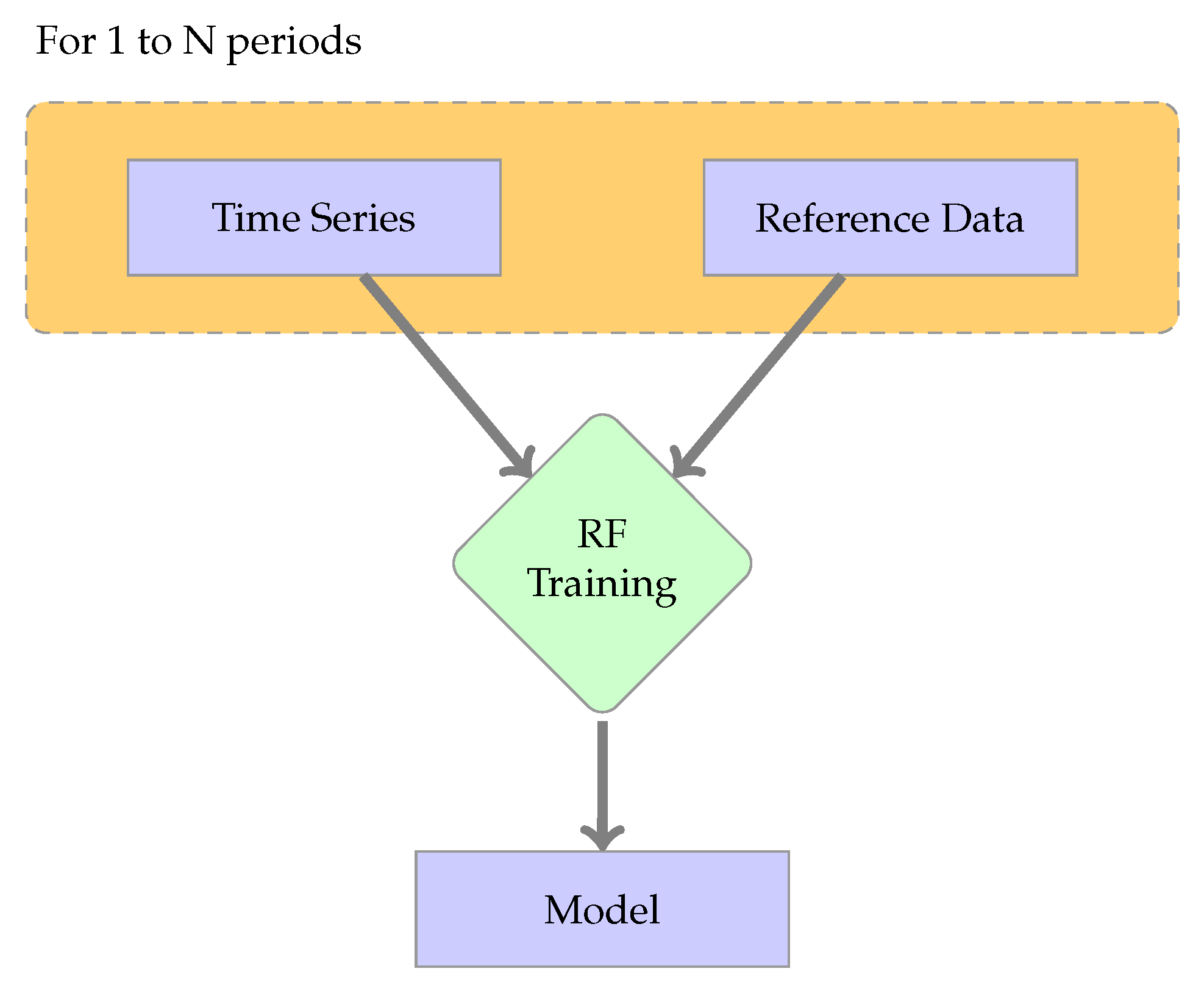
Figure 3.
Workflow of classification application. In the standard supervised case, the model is obtained by training the classifier with labeled samples of the current period image time series. In the other cases, the model is trained with labeled samples from previous period image time series.
Figure 3.
Workflow of classification application. In the standard supervised case, the model is obtained by training the classifier with labeled samples of the current period image time series. In the other cases, the model is trained with labeled samples from previous period image time series.

Figure 4.
Workflow of the post-processing chain. When only one classifier is used in Step 2 (standard supervised, naive or single classifier case), the labeled image is directly validated. For voting methods, each product of Step 2 is used according to the fusion rules.
Figure 4.
Workflow of the post-processing chain. When only one classifier is used in Step 2 (standard supervised, naive or single classifier case), the labeled image is directly validated. For voting methods, each product of Step 2 is used according to the fusion rules.

Figure 5.
Overall accuracy of each method for every period. The current period is displayed on the x-axis and the OA on the y-axis. This graph represents the OA of the standard Supervised (Sup), the Majority Voting (MV), the Confidence Voting (CV), the Single Classifier (SC), the Naive Baseline Mean (NBM), the Maximum of Naive Baselines (NBMax) and the Probability Voting (PV).
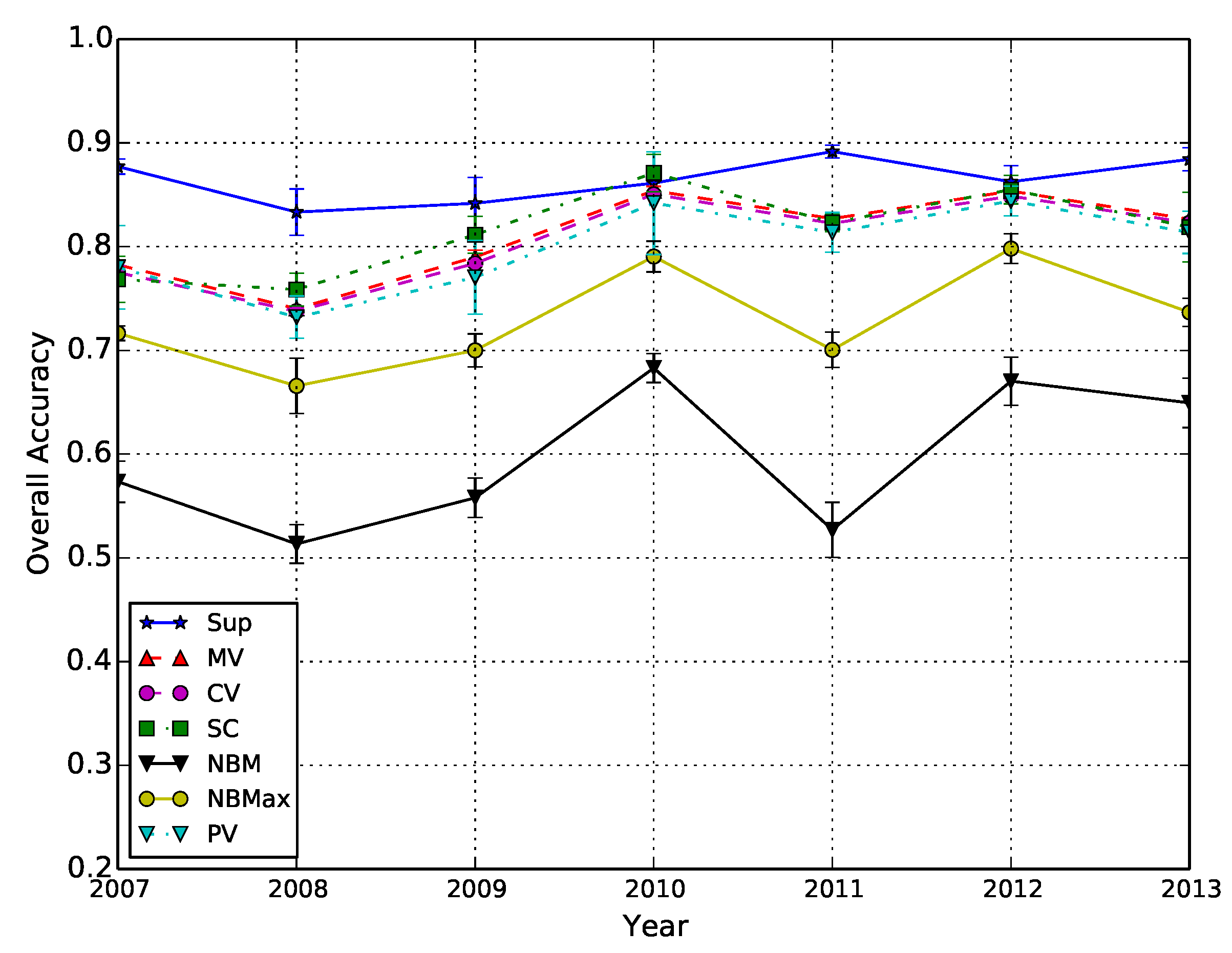
Figure 6.
Overall accuracy of each method for different numbers of time series available in the history. Each point represents the average of all runs for all possible subsets. The confidence interval represents 90% of the values obtained. The following abbreviations are used: MV, CV and PV for Majority, Confidence and Probability Voting, respectively, and SC for the Single Classifier; Sup and NBM for the standard Supervised and the Naive Baselines.
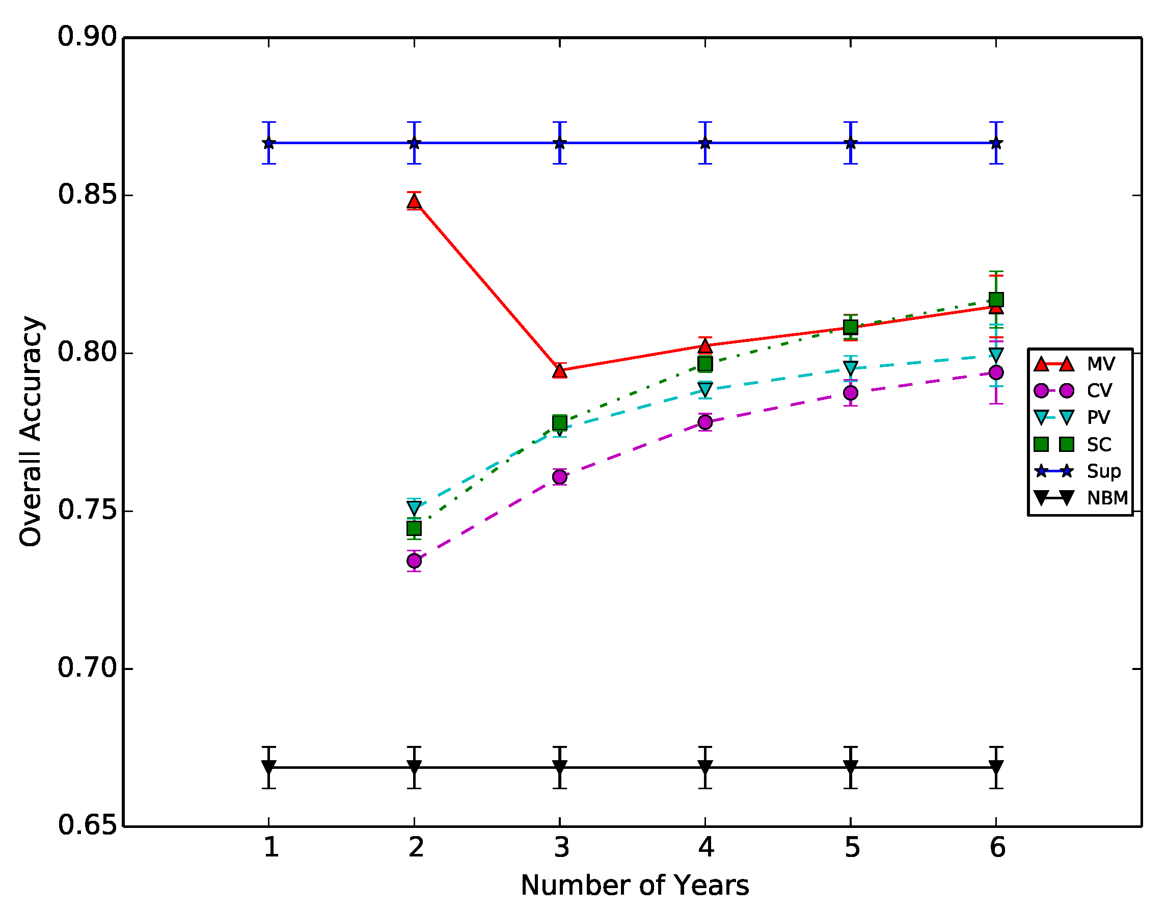
Figure 7.
Pixel distribution for each method and different size of history. For each method, we plotted the ratio of correctly classified (cc), incorrectly classified (ic) and undecided, i.e., not classified (nc). The dashed lines represent the limits defined by the standard supervised and naive cases.

Table 1.
Nomenclature and number of samples for each period.
| Number of Samples of Each Period | ||||||||
|---|---|---|---|---|---|---|---|---|
| Years | 2007 | 2008 | 2009 | 2010 | 2011 | 2012 | 2013 | |
| Classes | ||||||||
| Broad-leaved tree | 33,659 | 39,060 | 40,905 | 28,702 | 39,743 | 39,743 | 39,989 | |
| Pine | 10,160 | 13,112 | 6486 | 3703 | 3611 | 3611 | 3611 | |
| Wheat | 66,116 | 49,848 | 23,854 | 66,047 | 340,803 | 58,476 | 97,825 | |
| Rapeseed | 27,651 | 12,933 | 25,937 | 13,869 | 67,104 | 9885 | 40,508 | |
| Barley | 1937 | 5908 | 3564 | 1203 | 35,799 | 12,055 | 20,270 | |
| Maize | 58,438 | 39,185 | 49,570 | 54,858 | 142,214 | 29,063 | 105,107 | |
| Sunflower | 5851 | 19,952 | 19,489 | 24,215 | 237,662 | 23,107 | 29,544 | |
| Sorghum | 2040 | 1746 | 10,696 | 9829 | 8806 | 0 | 362 | |
| Soya | 754 | 7921 | 8816 | 6497 | 12,482 | 0 | 2308 | |
| Artificial Surface | 1550 | 1047 | 1047 | 1339 | 2089 | 1426 | 1496 | |
| Fallow land | 16,148 | 5145 | 3396 | 0 | 35,110 | 0 | 0 | |
| Wasteland | 1089 | 1299 | 9954 | 4142 | 10,357 | 10,357 | 14,208 | |
| River | 5806 | 9092 | 6825 | 6736 | 13,298 | 8850 | 10,071 | |
| Lake | 14,294 | 9997 | 10,090 | 20,070 | 4615 | 4440 | 4508 | |
| Gravel pit | 14,659 | 12,919 | 12,919 | 11,496 | 12,894 | 12,894 | 12,894 | |
| Hemp | 0 | 0 | 960 | 1806 | 5881 | 670 | 279 | |
| Grass | 42,656 | 11,900 | 13,571 | 18,379 | 120,299 | 21,182 | 25,858 | |
Table 2.
Overall accuracy obtained by the baseline cases. The rows represent the year of the data used to train the classifier, and the columns represent the year of the time series used to produce the map. On the diagonal, the standard supervised case is represented. The OA values and the confidence interval are computed using 10 different runs.
| Time Series | 2007 | 2008 | 2009 | 2010 | 2011 | 2012 | 2013 |
|---|---|---|---|---|---|---|---|
| Model 2007 | |||||||
| Model 2008 | |||||||
| Model 2009 | |||||||
| Model 2010 | |||||||
| Model 2011 | |||||||
| Model 2012 | |||||||
| Model 2013 |
Table 3.
Fscore obtained for all periods confounded by each method. The columns are: Sup for the standard Supervised case, MV for Majority Voting, CV for Confidence Voting, SC for Single Classifier, PV for Probability Voting and NB for the Naive Baseline case.
Table 3.
Fscore obtained for all periods confounded by each method. The columns are: Sup for the standard Supervised case, MV for Majority Voting, CV for Confidence Voting, SC for Single Classifier, PV for Probability Voting and NB for the Naive Baseline case.
| Class | Sup | MV | CV | SC | PV | NB |
|---|---|---|---|---|---|---|
| broad-leaved tree | ||||||
| pine | ||||||
| wheat | ||||||
| rapeseed | ||||||
| barley | ||||||
| maize | ||||||
| sunflower | ||||||
| sorghum | ||||||
| soybean | ||||||
| artificial surfaces | ||||||
| fallows | ||||||
| wastelands | ||||||
| river | ||||||
| lake | ||||||
| gravel pit | ||||||
| hemp | ||||||
| grass |
© 2017 by the authors. Licensee MDPI, Basel, Switzerland. This article is an open access article distributed under the terms and conditions of the Creative Commons Attribution (CC BY) license (http://creativecommons.org/licenses/by/4.0/).
Share and Cite
MDPI and ACS Style
Tardy, B.; Inglada, J.; Michel, J. Fusion Approaches for Land Cover Map Production Using High Resolution Image Time Series without Reference Data of the Corresponding Period. Remote Sens. 2017, 9, 1151. https://doi.org/10.3390/rs9111151
AMA Style
Tardy B, Inglada J, Michel J. Fusion Approaches for Land Cover Map Production Using High Resolution Image Time Series without Reference Data of the Corresponding Period. Remote Sensing. 2017; 9(11):1151. https://doi.org/10.3390/rs9111151
Chicago/Turabian StyleTardy, Benjamin, Jordi Inglada, and Julien Michel. 2017. "Fusion Approaches for Land Cover Map Production Using High Resolution Image Time Series without Reference Data of the Corresponding Period" Remote Sensing 9, no. 11: 1151. https://doi.org/10.3390/rs9111151
Note that from the first issue of 2016, this journal uses article numbers instead of page numbers. See further details here.