A Case Study of UAS Borne Laser Scanning for Measurement of Tree Stem Diameter
by

Martin Wieser
1,*, 
Gottfried Mandlburger
1,2,
Markus Hollaus
1,
Johannes Otepka
1,
Philipp Glira
1 and
Norbert Pfeifer
1
1
Department of Geodesy and Geoinformation, Technische Universität Wien, Gußhausstraße 27-29, 1040 Vienna, Austria
2
Institute for Photogrammetry, University of Stuttgart, Geschwister-Scholl-Str.24D, 70174 Stuttgart, Germany
*
Author to whom correspondence should be addressed.
Remote Sens. 2017, 9(11), 1154; https://doi.org/10.3390/rs9111154
Submission received: 23 August 2017
/
Revised: 25 October 2017
/
Accepted: 6 November 2017
/
Published: 10 November 2017
(This article belongs to the Section Forest Remote Sensing)
Abstract
:Diameter at breast height (DBH) is one of the most important parameter in forestry. With increasing use of terrestrial and airborne laser scanning in forestry, new exceeding possibilities to directly derive DBH emerge. In particular, high resolution point clouds from laser scanners on board unmanned aerial systems (UAS) are becoming available over forest areas. In this case study, DBH estimation from a UAS point cloud based on modeling the relevant part of the tree stem with a cylinder, is analyzed with respect to accuracy and completeness. As reference, manually measured DBHs and DBHs from terrestrial laser scanning point clouds are used for comparison. We demonstrate that accuracy and completeness of the cylinder fit are depending on the stem diameter. Stems with DBH > 20 cm feature almost 100% successful reconstruction with relative differences to the reference DBH of 9% (DBH 20–30 cm) down to 1.8% for DBH > 40 cm.
1. Introduction and Motivation
The distribution of tree diameter, measured at the breast height 1.3 m, is a fundamental parameter for characterization forest stands, including economic as well as ecologic aspects [1,2,3,4]. Direct measurement with calipers is labor intensive and only feasible for small sample plots, as typically used in forest inventories. Airborne laser scanning(ALS) has shown to be a mature technology for determining single tree position and height, but does not allow a direct observation of the diameter at breast height (DBH). Allometric functions relating tree diameter to height were used to map from tree height distribution to diameter distribution [5], but these functions have logarithmic nature and tree height gets into saturation while diameter may still increase. Terrestrial laser scanning, from tripods or mobile platforms [6] was suggested to automatically measure tree height and DBH, but this is again restricted to plots and hampered by accessibility. Still, those methods are operational and achieve accuracy in sub-dm level for DBH.
Unmanned aerial data acquisition gained popularity in the recent years, and close range Earth observation from the bird’s eye perspective became possible. One advantage of unmanned aerial systems (UAS) is that they can fly lower above the terrain than manned aircrafts, thus remote sensing instruments can acquire data at higher resolution. They can potentially be operated autonomously, thus decreasing costs. Earth observation with UAS was long restricted to small aircraft and therefore light weight instruments, using passive optical remote sensing [7].
Airborne laser scanning is advantageous for monitoring vegetation, because of its possibility to sample the tree canopy as well as the ground below and objects in between. In very dense ALS data, e.g., more than ten points per square meter, individual tree stems become visible and may be extracted automatically [8]. However, the flying height of ALS system has an impact on sampling distance and footprint diameter. With the advent of laser scanning on UAS, lower flying heights became operational [9]. Scanning LiDAR on board a UAS is described by [10], providing point clouds with a density of 60 points per m and a horizontal accuracy of 24 cm (RMS relative to ground control), and used in [11] for the detection of single trees. In [12] a system with similar properties with respect to point density and accuracy is described, also tested for single tree identification. Slightly lower performance was reported by [13] using a UAS with a payload of 100 kg.
Concerning accuracy, Glira, P. et al. [14] showed that using survey-grade scanner on an UAS does not offer advantages over standard airborne laser scanning from large, manned platforms. In any case, a higher point density can be achieved, and, therefore, the question arises, if additional forest parameters can be measured from the new data sources. Specifically, we want to answer the question if and how well tree diameter and diameter distribution can be measured from UAS borne laser scanning, and to evaluate its quality in terms of completeness, correctness, and accuracy. As a second question we investigate if ULS can replace TLS for DBH estimation.
2. Datasets
To answer the question if ULS can be a suitable data acquisition method for modeling stem diameters, a flight experiment in a complex alluvial forest was carried out. In the following subsections both the study area and the data capturing are described.
2.1. Study Area
The study area Neubacher Au (481250N, 152230E; WGS 84)is located at the lower course of the pre-alpine Pielach River (Lower Austria) near the confluence with the Danube. The area is subject to long-term monitoring and is described in detail in [15,16]. The site is part of the Natura2000 conservation area Niederösterreichische Alpenvorlandflüsse (Area code: AT1219000). We specifically focused on the alluvial forest enclosed by the meander bow shown in the central part of Figure 1 which features a very complex vegetation structure including woody debris as a result of recent flooding, lying and standing dead wood, dense under story and trees of different species. The tree heights vary between 10 and 35 m and the DBHs ranges up to 1 m.
2.2. Data Capturing
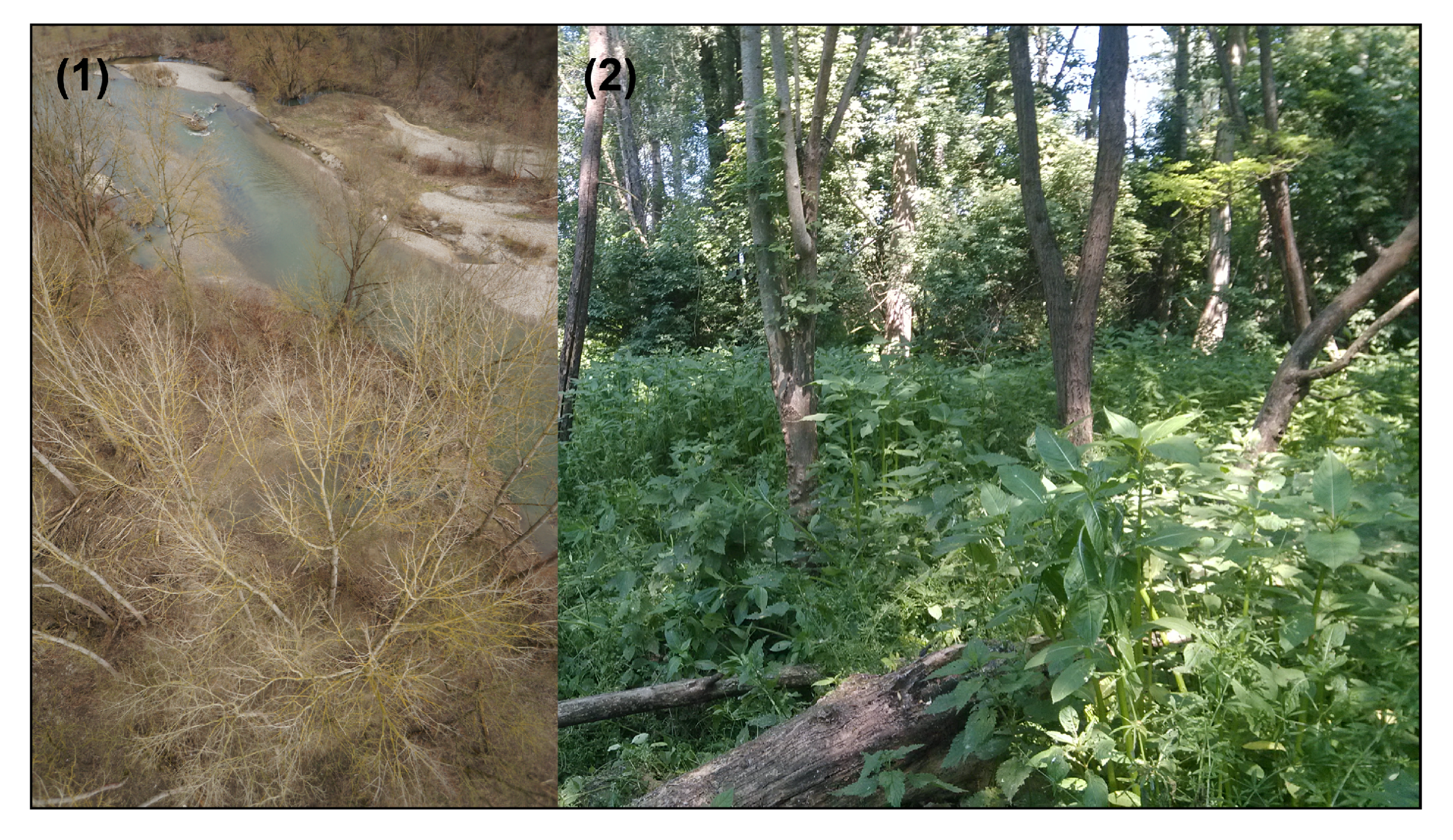
Data capturing was carried out on 26 February 2015 under leaf-off conditions (see Figure 2) with a Riegl VUX-SYS sensor mounted on a RiCOPTER UAS (RIEGL Laser Measurement Systems GmbH, Horn-Austria). The system consists of a Global Navigation Satellite System (GNSS), an Inertial Measurement Unit (IMU), the VUX-1 time-of-flight laser scanner, two 24 MPixel RGB cameras (Sony Alpha 6000) and a flight control unit. The carrier platform is an 9 kg X-8 array octocopter. The main frame is made of carbon-fibre and attached to it are four foldable arms, each of which carrying a coaxial array of two propellers. Including the batteries the maximum payload is 16 kg and at the maximum take-off mass of 25 kg the flight endurance is 30 min. The achievable altitude is higher than 150 m and, thus, restricted by national regulations for unmanned aircrafts. The effective measurement rate of the VUX-1 time-of-flight laser scanner is 350 kHz and the total field of view (FOV) is 230 [17]. The large FOV enables capturing vegetation both from above the canopy and from the side. The ranging accuracy of the sensor is 10 mm according to the vendor’s data sheet [18].
The flight crew consisted of a pilot and an additional operator responsible for flight mission guidance. After an GNSS/IMU initialization procedure, both static on the ground and dynamic after take-off, the UAS was autonomously flying a programmed path at a speed of 8 ms and an altitude of 50 m above ground, i.e., 15 m above the highest trees. Considering the beam divergence of the sensor the resulting laser footprint diameter was between 1 and 2.5 cm enabling detection of small vegetation objects. The acquisition of the area of interest was done with longitudinal strips (distance of 40 m) and cross strips on the block border. Furthermore two strips following the river are contained. The mission parameters resulted in a mean laser shot density of more than 1500 pts/m.
2.3. Reference Data
In order to validate the DBHs measures derived from the ULS point cloud field measurements with a flexible tape were done in June 2015. The circumference of 206 trees located in six circular plots of 12 m radius, see Figure 1 and Figure 2, were measured. The individual trees were identified and located based on field sketches and a high resolution near ground shaded relief map from the ULS with a resolution of 15 cm featuring the bare earth and the tree trunks. Near ground points where selected from 0 to 1.5 m above the DTM, which was also derived from the ULS as shown in Figure 4. This method was chosen as no GNSS signal was available at the forest ground due to leaf-on condition in the riparian forest. For the in situ measurements about 4 h were needed in the field to measure DBHs.
Moreover, data from a terrestrial laser scanner were captured in the area of plot 1 and 2 to compare the DBHs estimation of the ULS data from above with point clouds captured at ground. In total, nine TLS scan positions were obtained and oriented with circular retro reflecting targets placed in the TLS capturing area. The 3D positions of the reflectors were measured with a total station based on a control point network acquired by GNSS. In total, TLS and orientation measurements were taken in 3 h. The TLS data are used to validate if the ULS data is appropriate to model DBH in terms of quality, completeness and correctness compared to point cloud captured at ground with very high point density at breast height. For both ULS and TLS the same methods described later are applied to estimate DBH.
3. Methods
The methods for DBH estimation consisted of three major steps: (i) data preprocessing including thorough geometric calibration of the sensor system and derivation of a Digital Terrain Model (DTM); (ii) stem modeling via least squarest cylinder adjustment; and (iii) derivation of error metrics by comparing the results with in situ field measurements.
3.1. Geometric Sensor Calibration
Very high geometric quality of the 3D point cloud is of crucial importance as the DBH estimation relies on data from multiple flight strips. The redundant information contained in the strip overlap areas was therefore exploited to improve the fitting accuracy by means of strip adjustment [19]. For this purpose, the method presented in [14] was applied to the data. This method is formulated in a mathematically rigorous way, i.e., the functional model relies on the ALS sensor equation and the original scanner measurements (range and scan angle) and the trajectory measurements are used as input. Similar to the Iterative Closest Point (ICP) algorithm, the correspondences are established iteratively and directly between points of overlapping strips (avoiding a time-consuming segmentation and/or interpolation of the point clouds). Within the strip adjustment the ALS multi-sensor system is fully re-calibrated; this includes the estimation of the scanner calibration parameters (e.g., range finder scale error), the mounting calibration parameters (i.e., bore-sight misalignment and lever-arm), and the trajectory errors individually for each strip (i.e., GNSS and INS produce time depended errors). These parameters were estimated by minimizing simultaneously the point-to-plane distances of approx. 200,000 valid correspondences. The correspondences are uniform sampled in object space and only thus correspondences are eliminated which do not meet certain criteria as plane roughness, angle between normal vectors and point-to-plane distance. Therefore, correspondences are firstly located all over the block (ground, stems, branches, leaves...) but eliminated due to these criteria. Remaining correspondences are mostly located on ground, stems and bigger brunches. The final standard deviation of valid point-to-plane differences after the adjustment is 2.1 cm for the remaining correspondences. While the final relative accuracy of the a posteriori DEM height differences within smooth areas is 1.7 cm defined as 1. In Figure 3 one tree of plot 1 can be seen color coded by strip number. Based on the calibrated point cloud a DTM (shown in Figure 4) with a resolution of 15 cm was derived with the established method of hierarchic robust interpolation [20] which has proven to be especially well suited in vegetation areas [21]. In the following, only the points between 0.8 and 1.8 m above the DTM were used for modeling of the stems.
3.2. DBH Estimation
The DBH and exact tree position is estimated by cylinder fitting from the point cloud in three steps. (1) point selection; (2) refined parameter estimation (i.e., position and diameter); and (3) result validation. The cylinder parameters are estimated by robust least squares methods using the functional cylinder model described in [22]. The model consists of 5 parameters.
- a unit vector n pointing from the origin to the cylinder axis that is orthogonal to the cylinder axis (= two parameters using polar coordinates)
- the distance between cylinder surface and origin
- an angle defining the axis vector rotation around the aforementioned unit vector n
- the curvature of the cylinder (reciprocal of radius)
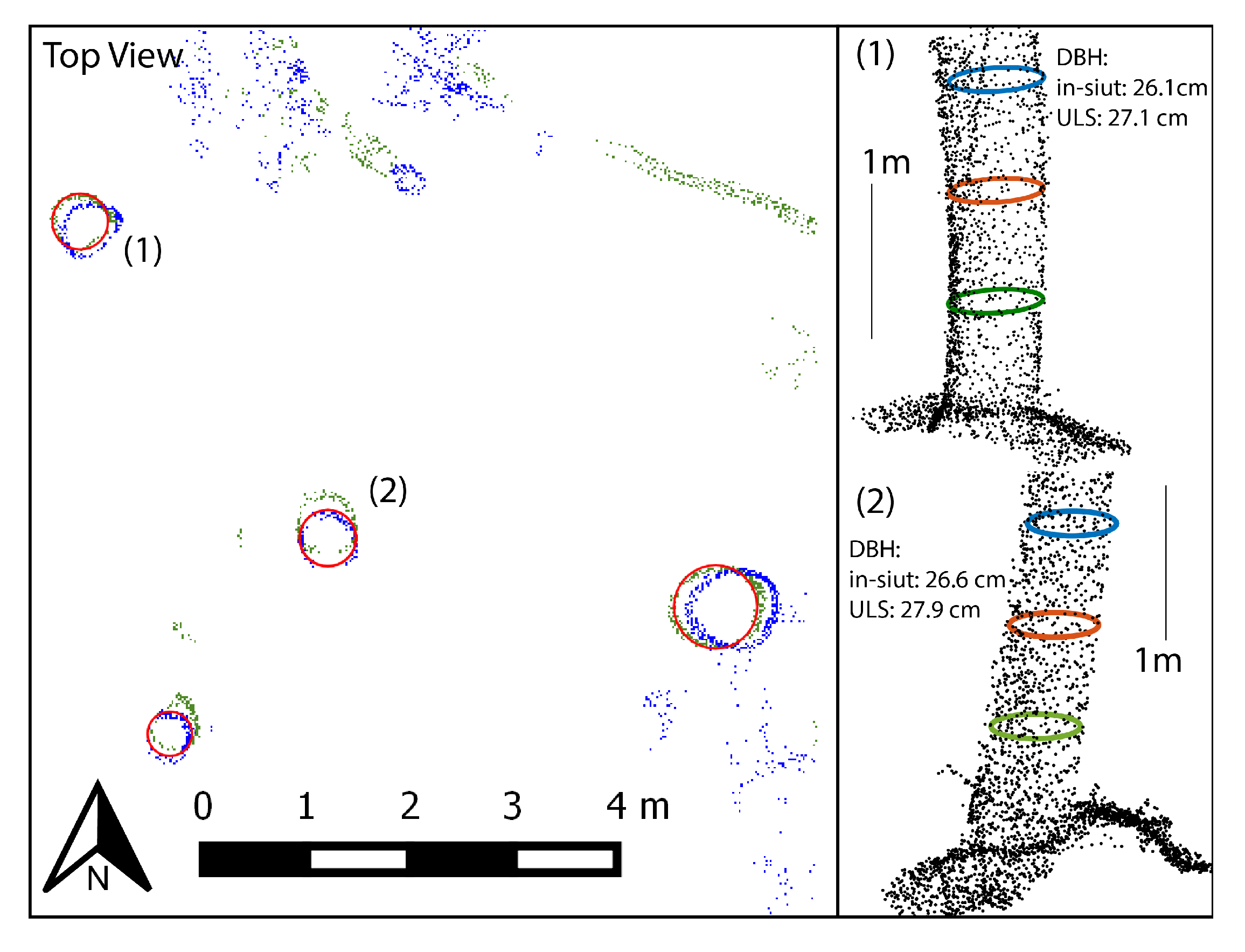
Which is a minimal parameter set for describing an arbitrary oriented cylinder in 3D. The primary question to be answered is, how well DBH can be measured, whereas the automatic detection of trees is not studied here. Instead a 1:1 relation between field measured and ULS derived tree (diameter) was manually selected based on the spatial co-location using a shaded relief map of ground and near ground points. These positions used for field identification, and cross sections of the point cloud (see Figure 5-TopView), provided approximate values for the cylinder fit.
As mentioned above, a robust least squares method was applied to eliminate outliers during the adjustment iterations. Based on the residuals (orthogonal distance to cylinder), points were re-weighted for the next iteration. After convergence points with higher absolute residuals than were marked as outliers and discarded in the final adjustment. Here, is the root mean square of the residuals. To achieve satisfactory results the selection of points that are used for the cylinder fit is crucial. If the selection window is chosen to small, relevant stem points may be discarded especially in case of tilted stems. On the other hand, larger selection regions may include a big number of non-stem related points from branches, leaves or shrub points causing the described robust estimation method to fail. Even though other robust estimation algorithms (e.g., RANSAC) maybe more tolerant against outliers, good approximation (stem axis in 3D and radius) are still essential if stems are closely surrounded by dense vegetation, like bushes and shrub. The estimated results were accepted if the adjustment converged and less than 50% of the points were classified as outliers.
3.3. Accuracy Assessment
Accuracy assessment of the UAS derived stem diameters is based on a comparison of the modeled stem diameters with the in situ measurements. The assessment focuses on: (a) modeling precision; (b) comparison of stem diameter modeled from ULS and TLS; and finally (c), the performance of the modeling is validated by comparing the stem diameter of ULS based results with those of the tape measurements. Tree wise as DBH differences and in form of a DBH distribution over all trees.
The results are analyzed based on standard statistics for both the modeling precision and accuracy. Whereas the precision is represented by the mean radial deviation of the LiDAR point from the fitted stem cylinder, the accuracy is obtained by comparing the deviations of the modeled and measured stem diameters DBH. While (a–modeling precision) characterizes the modeling itself (b and c) are a nominal-actual accuracy comparison under realistic conditions with TLS and tape measurements. Including data capturing errors, shortcomings of the modeling approach, and sub optimal data coverage due to occlusions from the upper canopy parts and curved stems. The comparison includes all stems measured in the field survey for which a valid circle could be modeled from the LiDAR points. Statistics (median, ) ( is the median of absolute differences from the median. ) are applied to different diameter classes (0–10 cm, 10–20 cm ...). Finally a stem diameter distributions for the field data and modeled stems are compared. DBH distribution is used in forestry for management and prediction of stem volumes. Therefore, a comparison is done how well the distribution of ULS fits to those from the tape measurements.
4. Results and Discussion
(a) Modeling precision
The precision measure (mean quadratic radial deviation) describes how well the LiDAR points fit to the estimated stem cylinder. This measure includes error components originating from the measuring process (uncertainties due to laser beam incidence angle, laser footprint, remaining geo-referencing errors) and from the object (slanted stems, irregular stem shapes). For 167 trees the cylinders was estimated successfully opposed to 39 stems which failed. This results in a 76.6% success rate for the cylinder fit itself (not taken into account wrongly estimated DBHs). The precision of the cylinder fit ranges from 9 mm to 59 mm with a median of 18 mm. Visual inspection of the selected stems has revealed that the deviations are dominated by stem irregularities (i.e., the stem shapes within the studied natural forest area deviate from the ideal circular model). Other influencing parameters causing increased radial deviations are irregularities along the stem axis within the considered stem section 0.8–1.8 m above ground). In Figure 5 a horizontal section of the ULS point cloud is displayed. Irregularities of the radial approximation to the stem and bending of the stem along the z-axis can be seen.
(b) Comparison ULS with TLS
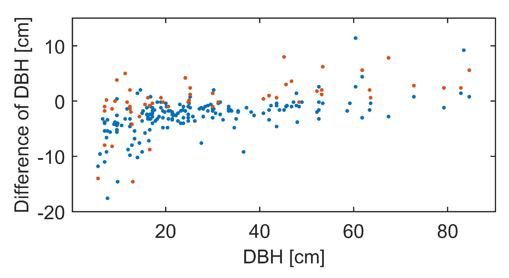
As the ULS is an airborne system which has to penetrate tree crowns to get points from the stems, the question of the modeling performance compared to high density data from the ground has to be addressed. Therefore, TLS data were captured at a high spatial resolution (mean point distance: 1 mm for points in the stem section of 0.8–1.8 m) and processed in the same way in order to compare modeling results of trees which are contained in, both, the ULS and TLS data set. The differences of the DBHs for the 57 trees which are contained in both (ULS and TLS) can be seen in Table 1. Differences defined as ULS-TLS. For 4 Of the 57 trees, gross differences in the cylinder fit have been found due to bad point coverage of the ULS or TLS. These 4 grossly wrong estimates had cm. From the results in Table 1 and the the differences seen in Figure 6 the only conclusion that can be drawn is that TLS performs for smaller trees better in terms of less outliers. Both datasets show scattered differences along the diameter distribution with the tendency of the ULS for an overestimation, which will be addressed later.
(c) Comparison of ULS with tape measurements
Table 2 shows the deviations of the DBH as measured in the field (tape measurements) and the DBH estimated from the ULS data for the entire in situ sample separated in diameter classes of 10 cm intervals. In Figure 6 the stem diameter differences are displayed for all trees where a cylinder fit was successful. Also here the challenge of small stem diameters can be observed. While for diameters >20 cm the success rate is near 100%, for smaller trees not only the success rate is much lower but also significant differences almost in the order of the stem size can be observed. Taking the relative differences compared to the DBH, it is clearly visible that for small stems the impact of failures is very high compared to the DBH result while for bigger stems over 30 cm DBH the relative difference is about 5% and lower. For small trees the main error source for the DBH estimation are uncertainties of the point cloud (e.g., strip adjust, ranging error), which almost in the size of half the radius. Effects of incidence angle and footprint size at small trees have as well an impact. As the footprint size is up to 2.5 cm the area illuminated is for small trees relatively strong bent. Thus the points are not longer scattered on the cylinder surface but tend to be spread within a cylinder instead on a cylinder surface. As well for stems with occlusions due to shadowing objects and trees only visible from one side the cylinder fit is not that robust for small stems in combination with all the above mentioned uncertainties.
While Outliers of bigger stems occur mostly result from bad ULS coverage of the stem. The cylindrical fitting tends to higher diameters if only a small portion of the stem is covered from one side. Under a stem diameter of 20 cm the success rate is only 40%. Another reason for outliers can be found disturbing objects. For example the high differences of −176 mm in Table 1 result from a small tree (DBH of 64 mm) surrounded strongly by shrub and branches and therefore the fit is using all the points inside a certain reach and cannot be estimated accurately.
Compared to both, TLS and in situ measurements, the cylinder model from the ULS tends to overestimate the DBH. For the in situ measurements an explanation could be that in situ DBH is taken at breast height with a single measurement. While the cylinder fit tends to higher values if the stem is conic in the stem range used for fitting. This can for example be seen in Figure 5 at tree (1) where in the upper part of the cylinder section the stem gets broader. For the TLS the conic form should have the same influence to the model as for the ULS. However, here a possible explanation could be the influence on the range estimation of the incidence angle at which the ULS laser beam hits the stems. Another explanation could be found in the very high resolution and small footprint of the TLS all small irregularity in the stem and bark will result in points towards the center, while the irregularities will be averaged by the ULS footprint. Figure 6 shows that systematic overestimation of DBH w.r.t. field reference occurs for ULS and DBH below 20 cm. Systematic errors for TLS are smaller.
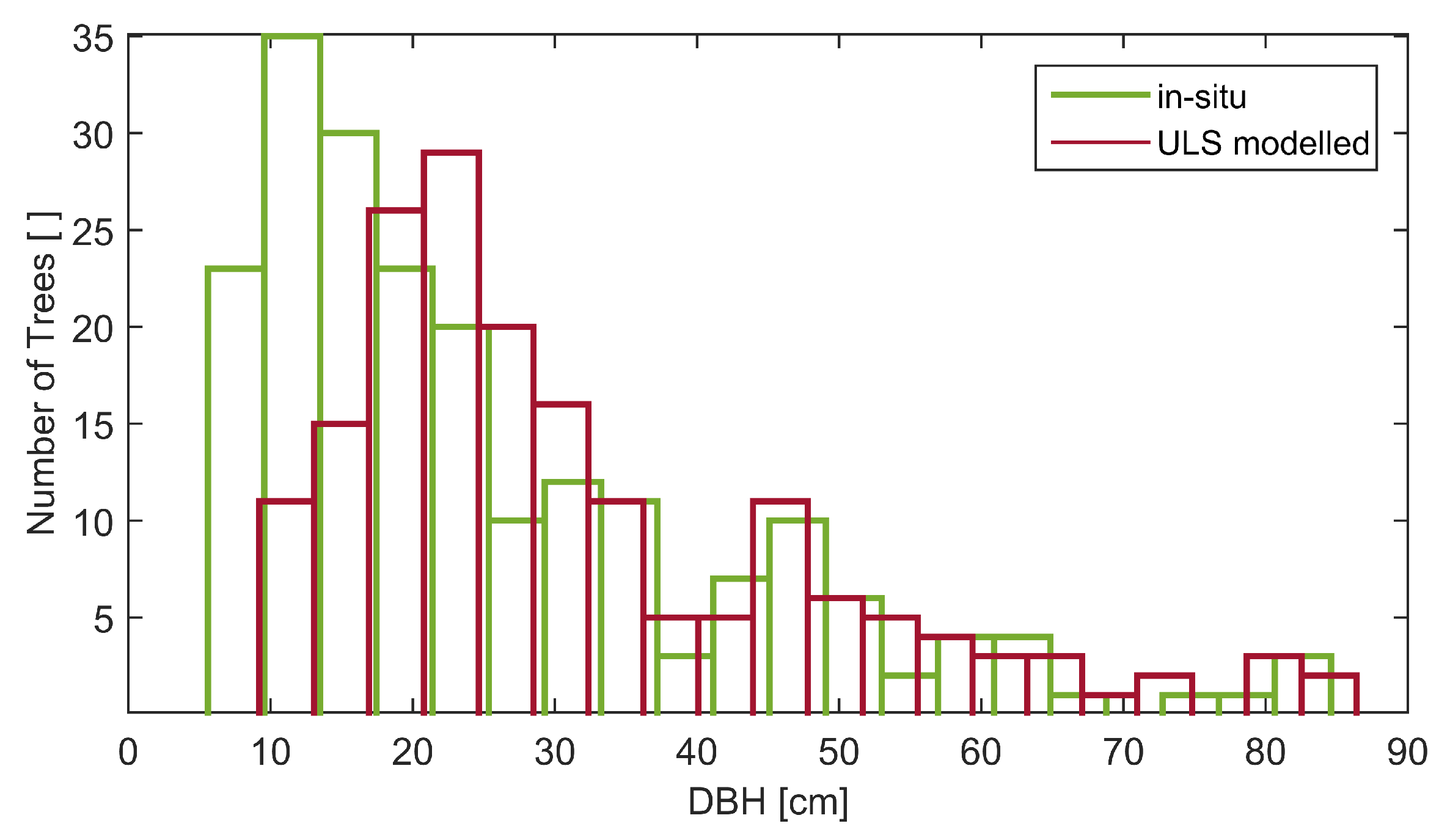
DBH distribution is used in forestry for management and prediction of stem volumes. Figure 7 shows the distribution of the in situ measured DBH (traditional circular plots) and the DBH distribution of the modeled ULS in the same plots. The DBH distribution of the ULS is classified in 3 classes: (1) Trees with DBH of lower than 20 cm are uncertain; (2) trees with DBH in the range between 20 and 35 cm can be both, correct fitted as well result from wrongly estimated DBH of small trees; and (3) trees with a DBH higher than 35 cm the distribution fits well and is quite stable.
As the success of the modeling is strongly depending on the amount of points at the tree stem, there are constraints to ULS. The data presented in this article was recorded in leaf-off condition with mostly deciduous trees. For leaf-on condition it can be much more challenging to derive appropriate point clouds. Still with the small footprint and high point density of the ULS it is depending on the density of the forest stand and foliage if enough stem points can be measured. As well the tree species, specially for coniferous trees, has its impact on the point cloud of stems. For the UAS recording session itself the weather is the most prominent factor determining if a UAS session can be performed, while classic tape measurements are performed in all weather conditions.
5. Conclusions and Outlook
We investigated the possibility to reconstruct tree DBH from point clouds acquired by UAS borne scanning LiDAR. A robust cylinder fit was applied to the points on the tree stems in six circular plots in an alluvial forest. [23] stated for the manual DBH measurements an accuracy of about 1.5%, which is almost the same level achieved here for the calculated DBH from the UAS LiDAR for trees with DBH > 30 cm. For small stems with DBH < 30 cm the DBH estimation becomes more challenging due to random and systematic errors, i.e., ranging accuracy and co-registration of the strips.
Using UAS LiDAR a high density point cloud of the stems can be derived due too the scan principle and the low flying altitude. Still occlusions can occur for dense forest structure or high stem density especially for tree species with stem bundles (e.g., willow, Salix sp.) at different locations. This lead, in our study, to overestimation of DBH, and in a few cases, inability to reconstruct the tree diameter.
Compared to TLS, DBH derived from the TLS perform better for small trees but still in TLS wrongly estimated DBHs are present. Both ULS and TLS show scattered differences over the DBH distribution. Concerning the time needed for data acquisition, ULS is lower. While in the forest TLS station numbers can be high and thus are very time consuming, the UAS can cover a larger area in the same duration. The time needed for the UAS session was about 5 h, including system preparation, test flight with a small UAS and data recording. On the other hand UAS has its drawback concerning weather conditions, tree species and foliage compared to tape measurements and TLS.
Overall, the higher the DBH the more accurate is the modeled DBH. We showed that for DBH > 35 cm the distribution of field measured and UAS LiDAR derived DBHs agree very well, below 20 cm the DBH measurements are uncertain, and in between, correct fitting and radius estimation results overlap with overestimation results for the diameter from smaller trees.
Acknowledgments
The work was supported by the Austrian Research Promotion Agency (FFG) COMET-K project “Airborne Alpine Hydro Mapping—From Research to Practice (AAHM-R2P)”.
Author Contributions
Martin Wieser and Gottfried Mandlburger conceived, designed and run the experiments and wrote the paper; Markus Hollaus and Norbert Pfeifer contributed scientific remarks ; Johannes Otepka and Philipp Glira contributed scientific tools.
Conflicts of Interest
The authors declare no conflict of interest.
References
- Lefsky, M.; Cohen, W.; Acker, S.; Parker, G.; Spies, T.; Harding, D. LiDAR remote sensing of the canopy structure and biophysical properties of Douglas-fir western hemlock forests. Remote Sens. Environ. 1999, 7, 339–361. [Google Scholar] [CrossRef]
- Naesset, E. Practical large-scale forest stand inventory using a small-footprint airborne scanning laser. Scand. J. For. Res. 2004, 19, 164–179. [Google Scholar] [CrossRef]
- Brassel, P.; Lischke, H. Eidgenössische Forschungsanstalt für Wald, Schnee und Landschaft. In Swiss National Forest Inventory: Methods and Models of the Second Assessment; WSL Swiss Federal Research Insitute: Birmensdorf, Switzerland, 2001. [Google Scholar]
- Gabler, K.; Schadauer, K. Methoden der Österreichischen Waldinventur 2000/02. 2006. Available online: https://bfw.ac.at/030/pdf/2414.pdf (accessed on 26 October 2017).
- Hara, T.; Kimura, M.; Kikuzawa, K. Growth Patterns of Tree Height and Stem Diameter in Populations of Abies Veitchii, A. Mariesii and Betula Ermanii. J. Ecol. 1991, 79, 1085–1098. [Google Scholar] [CrossRef]
- Holopainen, M.; Kankare, V.; Vastaranta, M.; Liang, X.; Lin, Y.; Vaaja, M.; Yu, X.; Hyyppä, J.; Hyyppä, H.; Kaartinen, H.; et al. Tree mapping using airborne, terrestrial and mobile laser scanning—A case study in a heterogeneous urban forest. Urban For. Urban Green. 2013, 12, 546–553. [Google Scholar] [CrossRef]
- Colomina, I.; Molina, P. Unmanned aerial systems for photogrammetry and remote sensing: A review. ISPRS J. Photogramm. Remote Sens. 2014, 92, 79–97. [Google Scholar] [CrossRef]
- Reitberger, J.; Schnörr, C.; Krzystek, P.; Stilla, U. 3D segmentation of single trees exploiting full waveform LiDAR data. ISPRS J. Photogramm. Remote Sens. 2009, 64, 561–574. [Google Scholar] [CrossRef]
- Michael, S.; Jung, J. LiDAR’s Next Geospatial Frontier—The state of LiDAR for UAS applications. GIM Int. 2015, 29, 25–27. [Google Scholar]
- Wallace, L.; Lucieer, A.; Watson, C.; Turner, D. Development of a UAV-LiDAR system with application to forest inventory. Remote Sens. 2012, 4, 1519–1543. [Google Scholar] [CrossRef]
- Wallace, L.; Lucieer, A.; Watson, C. Evaluating tree detection and segmentation routines on very high resolution UAV LiDAR Data. IEEE Trans. Geosci. Remote Sens. 2014, 52, 7619–7628. [Google Scholar] [CrossRef]
- Lin, Y.; Hyyppä, J.; Jaakkola, A. Mini-UAV-borne LiDAR for fine-scale mapping. IEEE Geosci. Remote Sens. Lett. 2011, 8, 426–430. [Google Scholar] [CrossRef]
- Nagai, M.; Chen, T.; Shibasaki, R.; Kumagai, H.; Ahmed, A. UAV-Borne 3-D Mapping System by Multisensor Integration. IEEE Trans. Geosci. Remote Sens. 2009, 47, 701–708. [Google Scholar] [CrossRef]
- Glira, P.; Pfeifer, N.; Mandlburger, G. Rigorous Strip Adjustment of UAV-based Laserscanning Data Including Time-Dependent Correction of Trajectory Errors. Photogramm. Eng. Remote Sens. 2016, 82, 945–954. [Google Scholar] [CrossRef]
- Mandlburger, G.; Hauer, C.; Wieser, M.; Pfeifer, N. Topo-Bathymetric LiDAR for Monitoring River Morphodynamics and Instream Habitats—A Case Study at the Pielach River. Remote Sens. 2015, 7, 6160. [Google Scholar] [CrossRef]
- Melcher, A.H.; Schmutz, S. The importance of structural features for spawning habitat of nase Chondrostoma nasus (L.) and barbel Barbus barbus (L.) in a pre-Alpine river. River Syst. 2010, 19, 33–42. [Google Scholar] [CrossRef]
- Mandlburger, G.; Hollaus, M.; Glira, P.; Wieser, M.; Milenkovic, M.; Riegl, U.; Pfennigbauer, M. First examples from the RIEGL VUX-SYS for forestry applications. In Proceedings of the SilviLaser, La Grande Motte, France, 28–30 September 2015; pp. 105–107. [Google Scholar]
- RIEGL Laser Measurement Systems GmbH. RIEGL VUX-1 Data Sheet. 2016. Available online: http://www.riegl.com/ (accessed on 26 October 2017).
- Toth, C.K. Strip adjustmentand registration. In Topographic Laser Ranging and Scanning: Principles and Processing; Shan, J., Toth, C.K., Eds.; CRC Press: Boca Raton, FL, USA, 2008; pp. 235–268. [Google Scholar]
- Kraus, K.; Pfeifer, N. Determination of Terrain Models in Wooded Areas with Airborne Laser Scanner Data. ISPRS J. Photogramm. Remote Sens. 1998, 53, 193–203. [Google Scholar] [CrossRef]
- Sithole, G.; Vosselman, G. Experimental Comparison of filtering algorithms for bare-earth extraction from airborne laser scanning point clouds. ISPRS J. Photogramm. Remote Sens. 2004, 59, 85–101. [Google Scholar] [CrossRef]
- Lukács, G.; Marshall, A.; Martin, R. Geometric Least-Squares Fitting of Spheres, Cylinders, Cones and Tori; Technical Report; Department of Computer Science, University of Wales: Cardiff, UK, 1997. [Google Scholar]
- Luoma, V.; Saarinen, N.; Wulder, M.A.; White, J.C.; Vastaranta, M.; Holopainen, M.; Hyyppä, J. Assessing Precision in Conventional Field Measurements of Individual Tree Attributes. Forests 2017, 8, 38. [Google Scholar] [CrossRef]
- Akerblom, M.; Raumonen, P.; Kaasalainen, M.; Casella, E. Analysis of Geometric Primitives in Quantitative Structure Models of Tree Stems. Remote Sens. 2015, 7, 4581–4603. [Google Scholar]
- Wang, D.; Kankare, V.; Puttonen, E.; Hollaus, M.; Pfeifer, N. Reconstructing Stem Cross Section Shapes from Terrestrial Laser Scanning. IEEE Geosci. Remote Sens. Lett. 2017, 14, 272–276. [Google Scholar] [CrossRef]
Figure 1.
Neubacher Au, Pielach River, Lower Austria; Hill shading of near ground DEM superimposed with colored point density map including UAS flight paths (yellow) and positions of sample plot areas (black circles).
Figure 1.
Neubacher Au, Pielach River, Lower Austria; Hill shading of near ground DEM superimposed with colored point density map including UAS flight paths (yellow) and positions of sample plot areas (black circles).
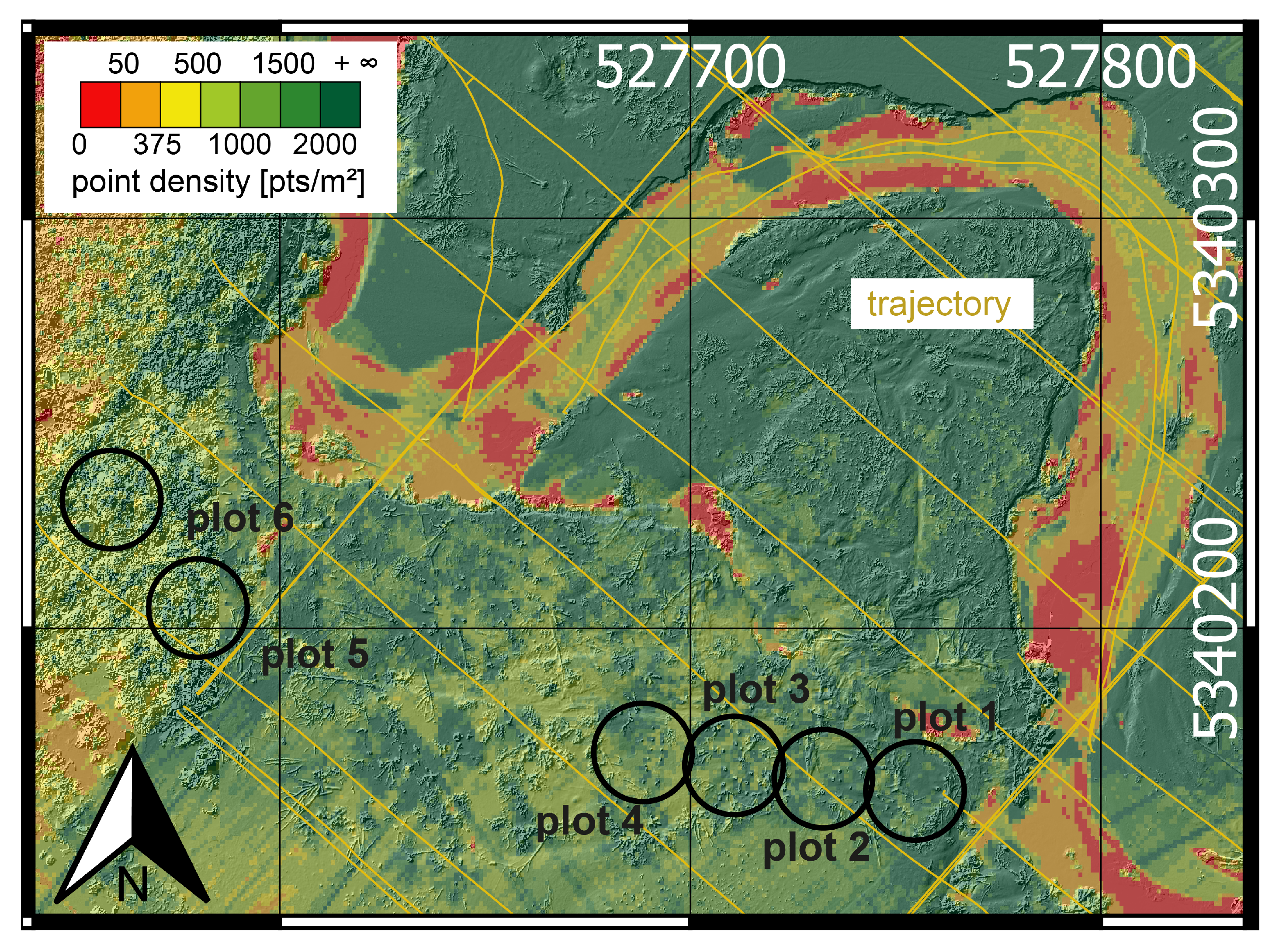
Figure 2.
(Left) Image from the UAV mounted camera showing the alluvial forest and the river Pielach in the background from February 2015. Location and viewing direction as seen in Figure 4; (Right) Image within the forest during the terrestrial field measurement campaign in June 2015.
Figure 2.
(Left) Image from the UAV mounted camera showing the alluvial forest and the river Pielach in the background from February 2015. Location and viewing direction as seen in Figure 4; (Right) Image within the forest during the terrestrial field measurement campaign in June 2015.

Figure 3.
Stripe wise color coded point cloud; (Top) Perspective view of tree stems; (Bottom) Top view of horizontal cross section as displayed in upper graphic with red box.
Figure 3.
Stripe wise color coded point cloud; (Top) Perspective view of tree stems; (Bottom) Top view of horizontal cross section as displayed in upper graphic with red box.
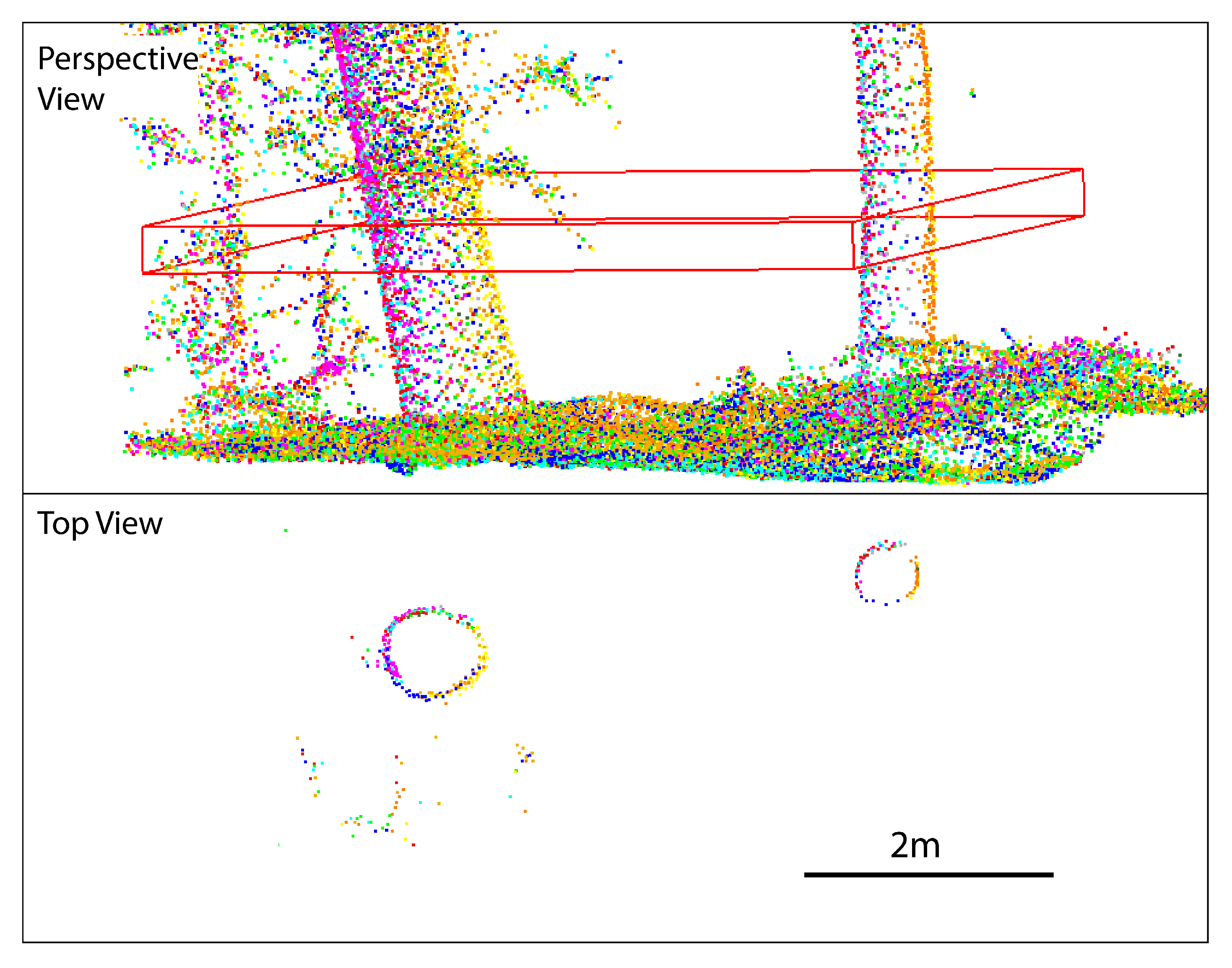
Figure 4.
Shading of the DTM derived by the ULS data. DTM resolution 15 cm. The orange box shows a zoom of the near ground DEM shaded relief map for plot 2. The viewing direction of Figure 2 (1) is marked in red.
Figure 4.
Shading of the DTM derived by the ULS data. DTM resolution 15 cm. The orange box shows a zoom of the near ground DEM shaded relief map for plot 2. The viewing direction of Figure 2 (1) is marked in red.
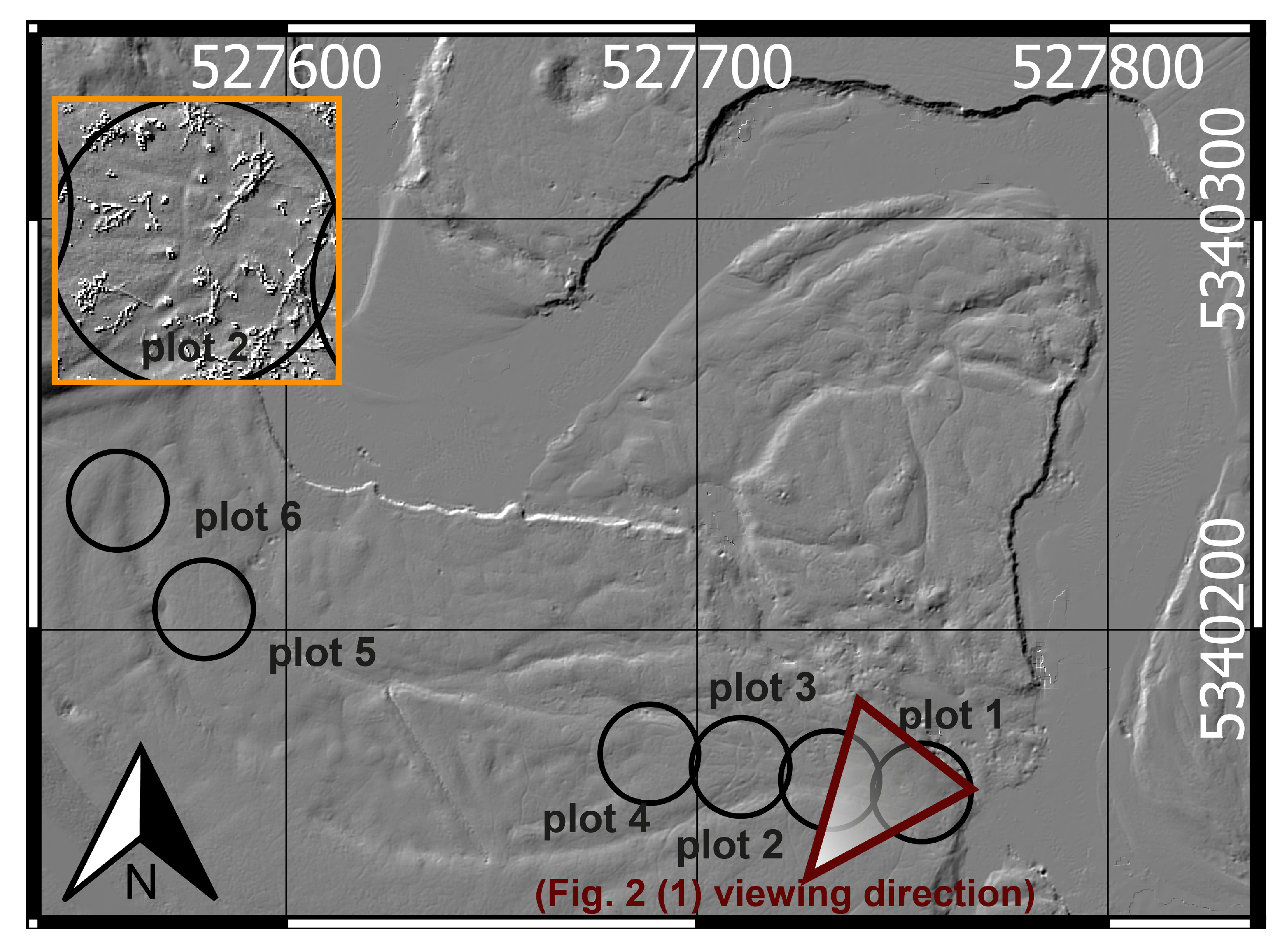
Figure 5.
Point distribution and resulting diameters; Left figure shows horizontal sections of the point cloud from heights of 0.8–1.2 m above ground (green) and 1.4–1.8 m above ground (blue). To indicate stem irregularities and stem bending. Red circles indicate DBH estimated with cylinder fit. On the right side for the tree (1) and (2) the point cloud of the ULS is shown with the cylinder: Red circle at DBH height. Green and blue for heights of 0.8 m and 1.8 m (limits of section used for fitting).

Figure 6.
DBH differences; in situ measurements minus cylinder fitting estimated DBH; blue: ULS modeled; red: TLS modeled.
Figure 6.
DBH differences; in situ measurements minus cylinder fitting estimated DBH; blue: ULS modeled; red: TLS modeled.

Figure 7.
DBH distribution; green: in situ measurements of circular plots; red: ULS DBH distribution within plots.
Figure 7.
DBH distribution; green: in situ measurements of circular plots; red: ULS DBH distribution within plots.


Table 1.
DBH model comparison between ULS and TLS. 57 trees are contained in both TLS and ULS.
| Nr. of Stems | Mean (mm) | Median (mm) | std. dev. (mm) | (mm) |
|---|---|---|---|---|
| all Trees contained in ULS and TLS | ||||
| 57 | 11 | 14 | 75 | 6 |
| without 4 gross differences | 15 | 14 | 19 | 5 |
| DBH 0–35 cm | ||||
| 36 | 23 | 13 | 49 | 5 |
| without 2 gross differences | 13 | 13 | 20 | 4 |
| DBH > 35 cm | ||||
| 21 | −11 | 18 | 100 | 8 |
| without 2 gross differences | 20 | 19 | 14 | 6 |
Table 2.
Nominal-actual comparison of in situ measured and from ULS modeled DBH (DBH differences: field minus ULS) for all available in situ measurements. “Stems failed” indicates that the cylinder fitting was not successful.
Table 2.
Nominal-actual comparison of in situ measured and from ULS modeled DBH (DBH differences: field minus ULS) for all available in situ measurements. “Stems failed” indicates that the cylinder fitting was not successful.
| Diameter (cm) | Stems Success | Stems Failed | min (mm) | max (mm) | Median (mm) | (mm) | Median (% of DBH) |
|---|---|---|---|---|---|---|---|
| 0–10 | 18 | 15 | −176 | 4 | −47 | 94 | 55.7 |
| 10–20 | 45 | 23 | −102 | 20 | −32 | 64 | 19.3 |
| 20–30 | 40 | 1 | −76 | 8 | −19 | 38 | 9.0 |
| 30–40 | 24 | 00 | −92 | 20 | −18 | 37 | 5.3 |
| 40–90 | 40 | 00 | −46 | 182 | −8 | 24 | 1.8 |
| 0–90 | 167 | 39 | −176 | 180 | −22 | 46 | 8.1 |
© 2017 by the authors. Licensee MDPI, Basel, Switzerland. This article is an open access article distributed under the terms and conditions of the Creative Commons Attribution (CC BY) license (http://creativecommons.org/licenses/by/4.0/).
Share and Cite
MDPI and ACS Style
Wieser, M.; Mandlburger, G.; Hollaus, M.; Otepka, J.; Glira, P.; Pfeifer, N. A Case Study of UAS Borne Laser Scanning for Measurement of Tree Stem Diameter. Remote Sens. 2017, 9, 1154. https://doi.org/10.3390/rs9111154
AMA Style
Wieser M, Mandlburger G, Hollaus M, Otepka J, Glira P, Pfeifer N. A Case Study of UAS Borne Laser Scanning for Measurement of Tree Stem Diameter. Remote Sensing. 2017; 9(11):1154. https://doi.org/10.3390/rs9111154
Chicago/Turabian StyleWieser, Martin, Gottfried Mandlburger, Markus Hollaus, Johannes Otepka, Philipp Glira, and Norbert Pfeifer. 2017. "A Case Study of UAS Borne Laser Scanning for Measurement of Tree Stem Diameter" Remote Sensing 9, no. 11: 1154. https://doi.org/10.3390/rs9111154
Note that from the first issue of 2016, this journal uses article numbers instead of page numbers. See further details here.