Article

Remote Sensing of 2000–2016 Alpine Spring Snowline Elevation in Dall Sheep Mountain Ranges of Alaska and Western Canada

1
School of Natural Resources and Extension, University of Alaska Fairbanks, Fairbanks, AK 99775, USA
2
Yukon Department of Environment, Whitehorse, YT Y1A 4Y9, Canada
3
College of Earth, Ocean and Atmospheric Sciences, Oregon State University, Corvallis, OR 97331, USA
4
School of Environmental and Forestry Sciences, University of Washington, Seattle, WA 98195, USA
5
Scenarios Network for Alaska and Arctic Planning, University of Alaska Fairbanks, Fairbanks, AK 99775, USA
*
Author to whom correspondence should be addressed.
Remote Sens. 2017, 9(11), 1157; https://doi.org/10.3390/rs9111157
Submission received: 18 August 2017 / Revised: 6 November 2017 / Accepted: 7 November 2017 / Published: 11 November 2017

Abstract

:
The lowest elevation of spring snow (“snowline”) is an important factor influencing recruitment and survival of wildlife in alpine areas. In this study, we assessed the spatial and temporal variability of alpine spring snowline across major Dall sheep mountain areas in Alaska and northwestern Canada. We used a daily MODIS snow fraction product to estimate the last day of 2000–2016 spring snow for each 500-m pixel within 28 mountain areas. We then developed annual (2000–2016) regression models predicting the elevation of alpine snowline during mid-May for each mountain area. MODIS-based regression estimates were compared with estimates derived using a Normalized Difference Snow Index from Landsat-8 Operational Land Imager (OLI) surface reflectance data. We also used 2000–2009 decadal climate grids to estimate total winter precipitation and mean May temperature for each of the 28 mountain areas. Based on our MODIS regression models, the 2000–2016 mean 15 May snowline elevation ranged from 339 m in the cold arctic class to 1145 m in the interior mountain class. Spring snowline estimates from MODIS and Landsat OLI were similar, with a mean absolute error of 106 m. Spring snowline elevation was significantly related to mean May temperature and total winter precipitation. The late spring of 2013 may have impacted some sheep populations, especially in the cold arctic mountain areas which were snow-covered in mid-May, while some interior mountain areas had mid-May snowlines exceeding 1000 m elevation. We found this regional (>500,000 km2) remote sensing application useful for determining the inter-annual and regional variability of spring alpine snowline among 28 mountain areas.

Graphical Abstract

1. Introduction

Climate warming is altering the duration, amount and timing of snowfall and these changes are especially substantial in arctic and boreal regions [1]. Changing spring snow conditions likely impact many alpine mammals. For example, earlier spring plant phenology initiated earlier emergence from hibernation, earlier weaning, increased body mass and increased survival in yellow-bellied marmots (Marmota flaviventris) [2]. Reduced snow depth during calving allowed parturient caribou (Rangifer tarandus) females to disperse up in elevation away from predator populations, thus increasing recruitment rates [3]. During later springs, upward movement may be limited by snow, resulting in higher predation rates on neonates [3]. In addition, late-winter snowfall has been shown to negatively affect caribou calf growth rates in Alaska [4].
Dall sheep (Ovis dalli dalli) are an iconic alpine species distributed across northwestern North America, including major mountain ranges in Alaska, Yukon, the Northwest Territories and northwest British Columbia. The species is a rare example of a North American large mammal that occupies most of its native range , with genetic isolation among mountain range populations for thousands of years [5]. Because there is limited dispersal among mountain populations, some populations may be vulnerable as “island populations”. There are many survival challenges in these high latitude mountains including extreme weather events such as heavy snowfall, winter icing events and late spring snow delaying spring forage production [6,7] (Figure 1).
Dall sheep populations have declined in recent decades in some areas. Range-wide, Dall sheep populations have declined by 21% since 1990 [8] but the causes remain unknown [9]. Harsh spring weather was shown to reduce horn growth rates in the Yukon [10] and pregnant Dall sheep in Denali National Park were found to avoid snow-covered areas [11]. However, no studies have examined impacts of spring snow conditions on Dall sheep populations across their range, in part due to a lack of available regional snow products that capture important features of snow-covered landscapes, such as the elevation of spring snowline.
The elevation of spring snowline is important to all alpine herbivores in this region since above this elevation forage is restricted to low quality forage and is covered with snow. Below snowline, snowmelt has occurred and new shoot growth provides high quality forage that is available for the first time after a long winter. The snowline elevation may thus affect sheep by altering the quantity and quality of forage. Snowline elevation may also affect the food-safety tradeoff for sheep, because several of their primary predators occur mainly at lower elevations [12].
A spring warming trend has occurred in recent decades with earlier spring snowmelt and river and lake ice-out in northern Alaska and Canada [13,14,15]. However, despite this trend in earlier spring snowmelt, an occasional late spring could impact sheep populations in some mountain ranges. Spring 2013 was unusually late at lower elevations, with river ice-out in Canada and interior Alaska occurring 11–20 days later than the 22-year average (Figure 2). Snow conditions and impact on lamb survival in the spring of 2013 likely varied among mountain areas. Increased variability in inter-annual alpine snow may impact populations to a greater extent than shifting mean conditions and additional tools and products are therefore needed to characterize this variability across broad regions [16].
Dall sheep inhabit a wide range of alpine areas in Alaska and western Canada, ranging from arctic tundra alpine areas north of latitudinal tree line, to alpine areas where glaciers dominate the landscape, to relatively warm alpine areas. How does winter precipitation and spring temperature vary among these alpine areas?
Objectives of this research were to:
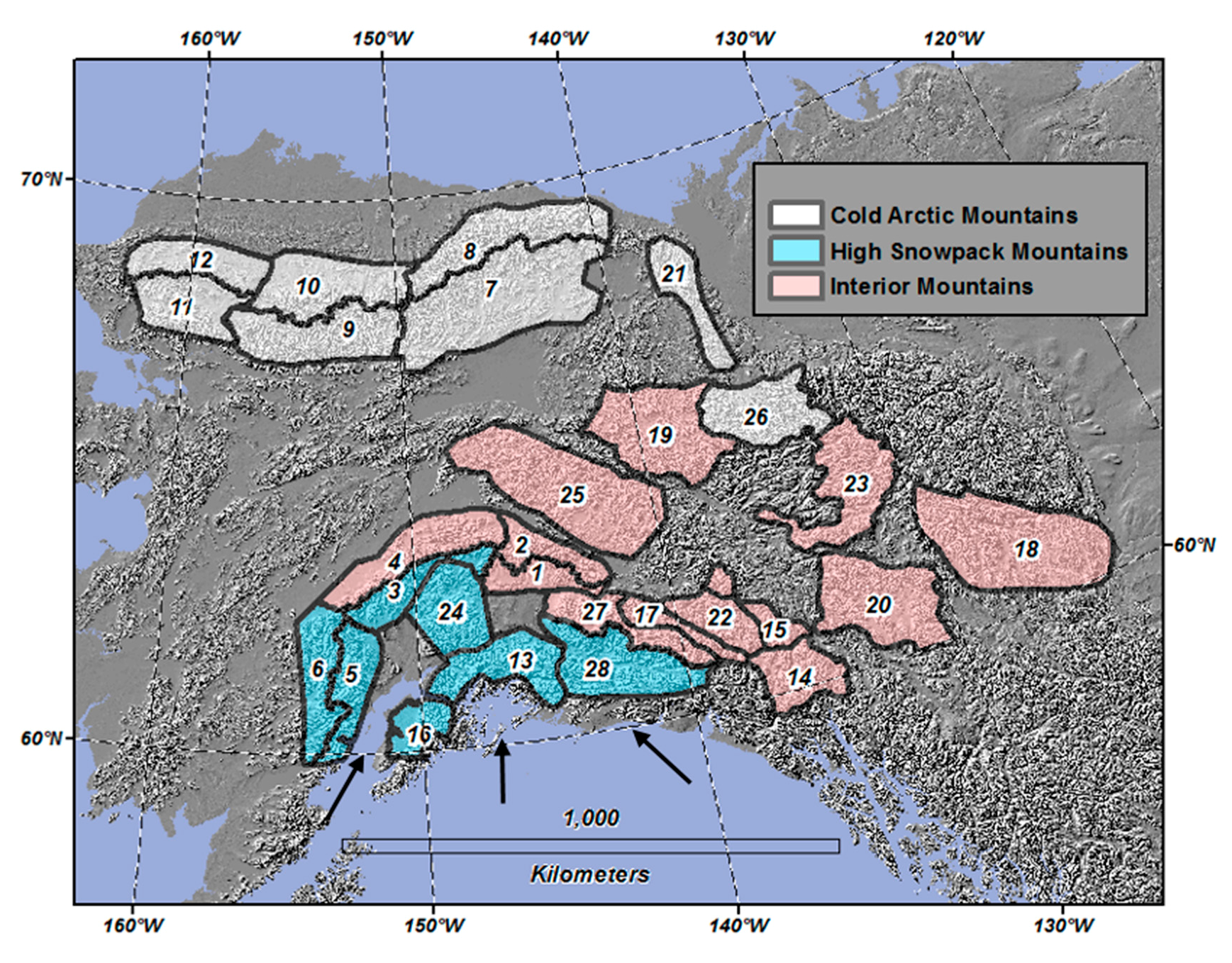
  • Use gridded climate products to estimate winter precipitation and May temperature among 28 major mountain areas in Alaska and northwest Canada.
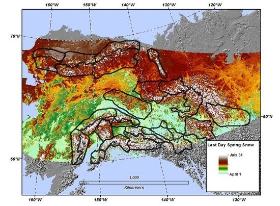
  • Develop 2000–2016 remotely sensed estimates of spring snowline elevation during the typical lambing period of mid-May among the 28 major mountain areas.
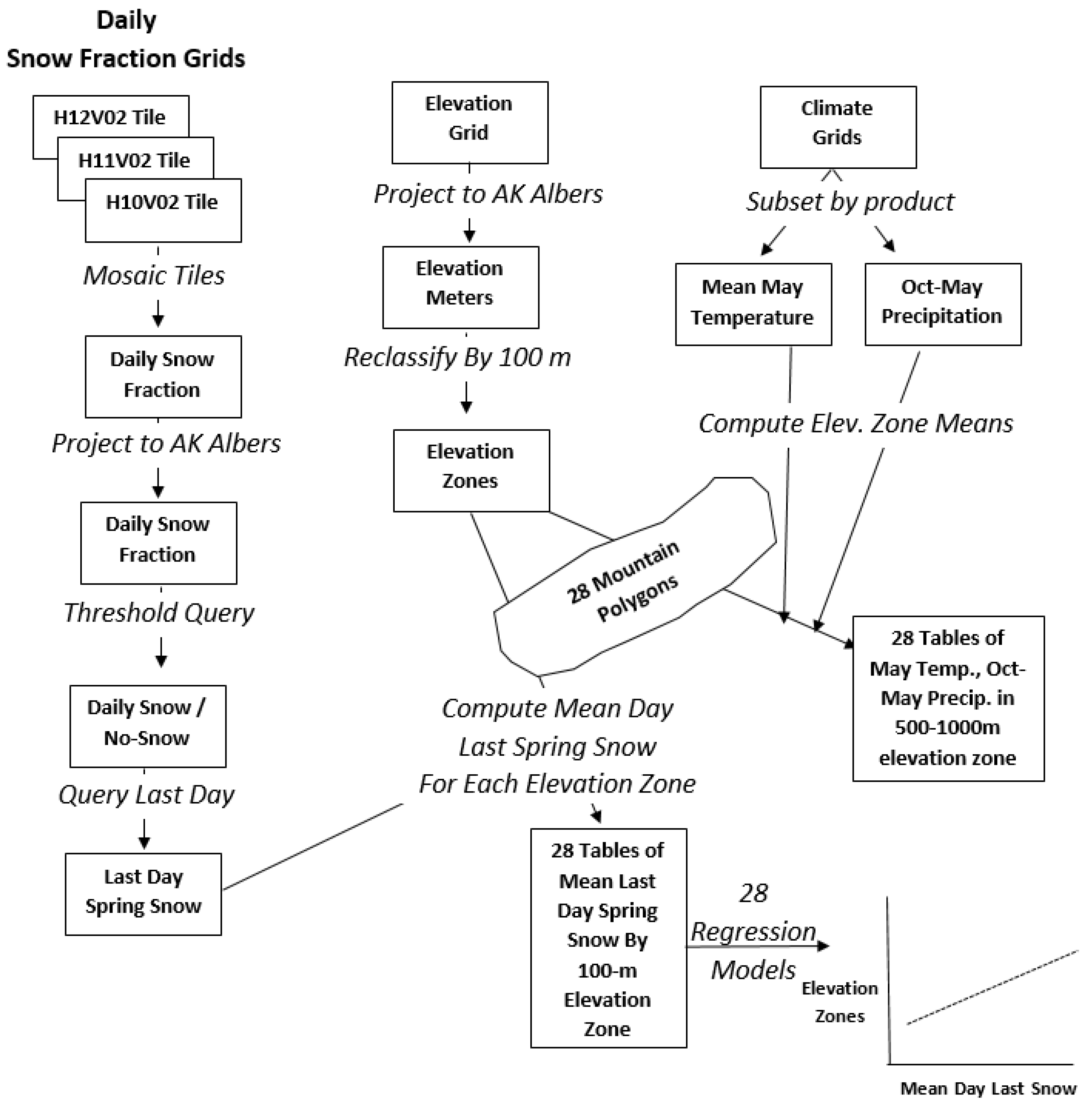
  • Model mean 2000–2016 spring snowline elevation as a function of decadal mean winter precipitation and mean spring temperature.
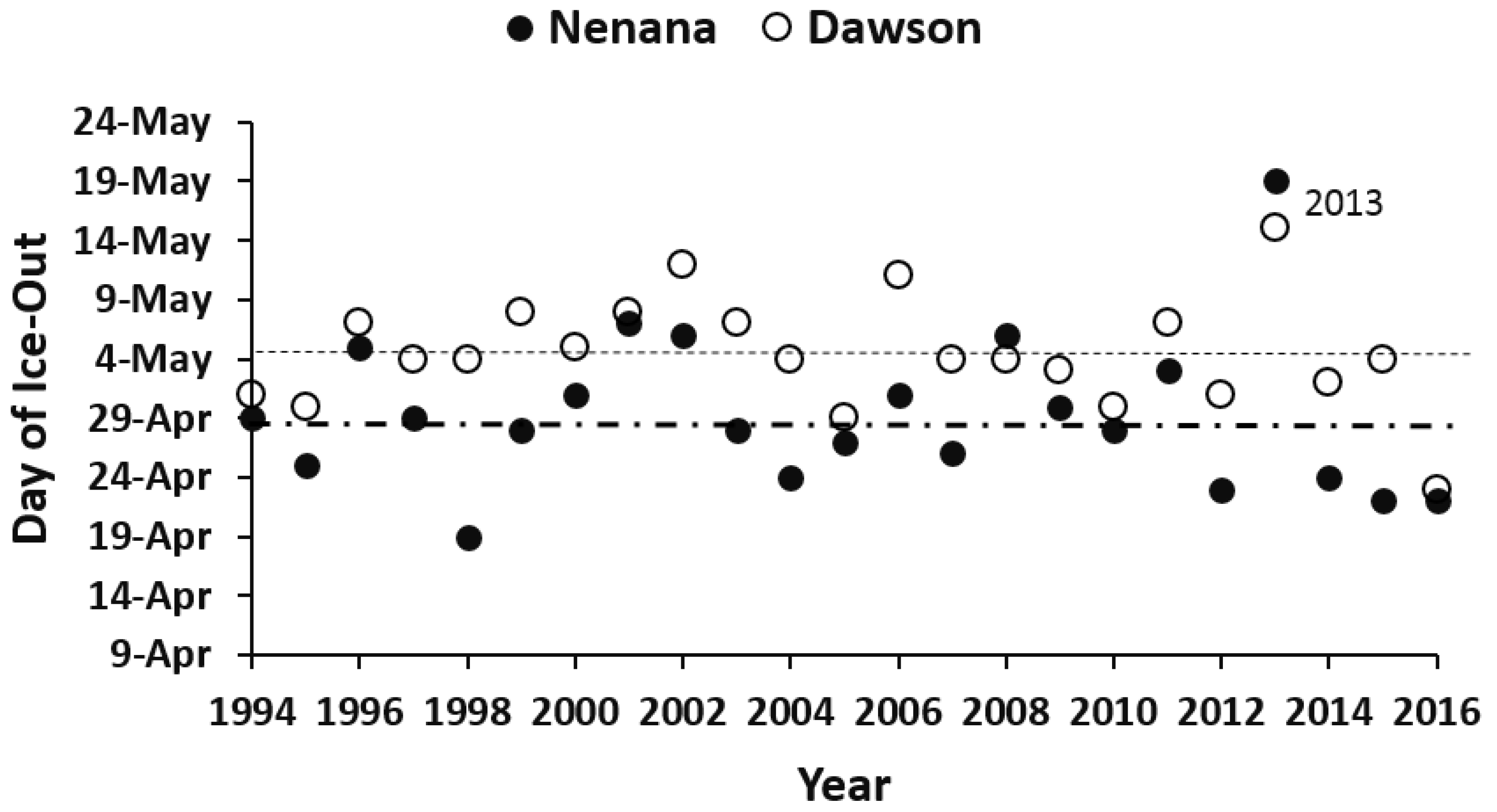
  • Assess the regional variability of remotely sensed spring snowline during the unusually cold and late spring of 2013.
Regional snowline estimation varies with application such as the lowest elevation of alpine snow at the end of the summer [17] or the equilibrium line altitude for estimation of glacier mass balance [18]. Spring snowline is the regional elevation where at lower elevations snowmelt has occurred. In the French Alps spring snowline was estimated using a time series of MODIS data as locations with first snow-free day with an uncertainty of ± 3 days [19]. In Slovakia, a time series of daily MODIS snow cover was used to estimate snowline as the elevation for which the area of snow pixels below and non-snow pixels above is minimized for each day [20]. The method was above 75 percent accurate during spring months when compared to field data, however the method may not be applicable to regions where perennial glaciers below the regional snowline would be misclassified as snow pixels each day. In this study we use a regression approach to estimate the spring regional snowline elevation across 28 mountain areas for 17 years. This application may be useful for examining the inter-annual and regional effects of changing spring snowline on alpine wildfire populations.

2. Methods

2.1. Study Region

The study region included major Dall sheep mountain areas across northwestern North America, which encompasses this species’ global distribution. Dall sheep generally inhabit the elevation zone at or above tree line in arctic and subarctic mountains where they typically feed in alpine meadows near steep, rocky slopes that serves as escape terrain from predators such as wolves, coyotes and bears. The study region included 28 alpine areas (Table 1) in Alaska, Yukon, the Northwest Territories and British Columbia in Canada. Because of a maritime to continental climate gradient, we delineated several study areas within the Alaska Range, Brooks Range and Wrangell mountains. Typically, spring snowline is at lower elevations on the south side relative to the north side of the Alaska Range and Wrangell mountains due to the maritime influence of the Pacific Ocean. Both the Alaska and Brooks Range have a west-to-east gradient of maritime to continental climate, with spring snowline typically at lower elevation in western portions of these ranges (Figure 3).

2.2. Climatic Variation among Mountain Areas

Based on well-known regional climate [21,22,23], we grouped our mountain areas into 3 classes (Figure 3): (1) cold arctic mountains; (2) high snowpack mountains; and (3) interior mountains. These cold arctic mountains were within the global tundra biome, with a monthly mean May temperature of 4 °C or less (Table 1). The other mountain areas were within the global boreal forest biome [24]. The high snowpack mountain areas intercept winter moisture from the Pacific Ocean air mass flow associated with the Aleutian Low, resulting in heavy winter snow accumulation and substantial alpine glaciers. The interior mountain areas receive less Pacific Ocean air mass flow, resulting in a more continental climate with lower precipitation, warmer spring/summer temperatures and most of these mountains lack glaciers. Mountain areas from the high snowpack class had winter precipitation ranging from 326–936 mm, while mountain areas from the interior mountain class ranged from 84–254 mm (Table 1).
The elevation of spring snowline is dependent on the depth of snow pack accumulated over the winter and spring temperature above freezing. Therefore, we expected spring snowline elevation to vary with the amount of snow accumulated over the winter (October–April) and with spring temperature. We created 2-km grids of winter precipitation and mean May temperature from the most recent decade of 2000–2009 for each of the 28 mountain areas. Gridded climate data were not available for the entire study region after 2009. These grids were based on 0.5 degree monthly climate products (Climate Research Unit—CRU TS 3.1) [25] which were downscaled by the Scenarios Network for Alaska and Arctic Planning (SNAP) program at the University of Alaska Fairbanks [26]. These products were downscaled via the delta method [27,28] using Param-elevation Relationships on Independent Slopes Model (PRISM) [29] with 1961–1990 2-km resolution climate normals (monthly temperature and precipitation) as baseline climate. The delta method was implemented by calculating climate anomalies applied as differences in temperature and quotients in precipitation, between monthly CRU data and PRISM climate normals for 1961–1990. These coarse-resolution anomalies were then interpolated to PRISM spatial resolution via a spline technique and then added to (temperature) or multiplied by (precipitation) the PRISM climate normals. The PRISM climatology product was used as baseline climate in the downscaling procedure because it accurately represents the elevational effects on precipitation patterns across mountainous regions [30] and it is based on extensive use of weather stations across Alaska: 455 for precipitation, 316 for temperature, as well as the European Center for Medium-range Weather Forecasts’ reanalysis of temperatures at the 500 mb height [31].
We used the 2-km decadal climate grids to estimate the mean May temperature and total October–April precipitation for each of the 28 areas (elevation zone from 500–1000 m). Virtually all October–April precipitation in these areas is snow. We then developed a linear model predicting MODIS-based mean 15 May snowline elevation (see Section 2.4) as a function of decadal mean May temperature and October–April precipitation.

2.3. Elevation Zones

To delineate alpine elevation zones, we used the Global Multi-resolution Terrain Elevation Data 2010 produced by the U.S. Geological Survey (USGS) and the National Geospatial-Intelligence Agency (NGA) (http://earthexplorer.usgs.gov) at 30 arc second spacing. To match the other geospatial datasets, the elevation data were projected to the Alaska Albers NAD83 coordinate system using bilinear interpolation to 500-m pixel size. For each mountain range, we then created a raster of elevation zones at 100-m elevation intervals. These elevation zone grids were used with the time series of daily remotely sensed snow fraction to estimate the mean day of year of last spring snow for each zone.

2.4. Remotely Sensed Snow Fraction

We used a daily snow fraction product, from the Moderate Resolution Imaging Spectrometer (MODIS) sensor that covered our entire study area at 500-m pixel size (global tiles H10V02, H11V02, H12V02). The MODIS Snow-Covered Area and Grain size product (MODSCAG) adapts methods originally developed from imaging spectrum [32] to use the spectral information from MODIS to estimate subpixel snow properties—fractional snow-covered area, grain size and albedo. The MODSCAG snow fraction product has been validated with fractional snow cover derived using Landsat sensors [33] resulting in a root mean squared error of 5% averaged across 31 Landsat scenes. This product is superior to the MOD10A1 snow extent products, especially during the period of spring snowmelt [34].
The physically-based MODSCAG algorithm uses spectral mixture analysis on a pixel-by-pixel basis to derive gridded 500 m daily fraction of snow cover estimates. The linear spectral mixture procedure is based on land surface endmembers (e.g., snow, soil, rock, vegetation, lake ice) that matches surface reflectance from the Terra MOD09GA (MODIS daily gridded surface reflectance) product. The MODSCAG model uses the relative shape of the snow’s spectrum and is applicable to mountainous areas where the local solar illumination angle on a slope is often unknown because of co-registration errors between the image and a digital elevation model. The MODSCAG model estimates the fraction of each pixel that is covered by snow [33]. A threshold value of >0.15 to flag each daily 500-m pixel as snow covered has been used to accurately map snow extent for treeless areas in the Colorado Rocky Mountains, upper Rio Grande, Himalayas in Nepal [35] and the Sierra Nevada Mountains in California [36]. Based on these results, we used a fraction threshold value of >0.15 to flag each daily 500-m pixel as snow covered.
For 2000 through 2016, the three daily snow fraction tiles were mosaicked to one daily grid, covering the entire study area. The daily snow fraction grid was then projected to the Alaska Albers NAD83 projection using nearest neighbor resampling at 500-m pixel size to match the other geospatial datasets. For each day from 1 April through 31 July, each 500-m pixel was flagged as “Snow” if the snow fraction exceeded 0.15, resulting in a time series of daily snow grids. Any pixel that did not have a valid snow fraction value (primarily due to cloud contamination) was excluded from analysis. From this daily time series, the last day of snow grid was computed as day of year ranging from 91 (1 April) to 213 (31 July) for each pixel. Any pixel with snow detected on 1-August was likely from perennial snowfields or glaciers and these pixels were excluded from the analysis. For each day from 1 April through 31 July, each 500-m pixel was flagged as “Snow” if the snow fraction exceeded 0.15, resulting in a time series of daily snow grids. From this time series, the last day of snow grid was computed as day of year ranging from 91 (1 April) to 213 (31 July) for each pixel (Figure 4).
For each 100-m elevation zone with at least 1000 pixels, the mean day of year of last spring snow was then computed. We used a sample threshold of 1000 pixels to minimize local effects in smaller elevation zones that were from in a mountain area.
For each of the 28 mountain areas, we estimated the May snowline elevations by regression equations predicting the elevation of last snow as a function of mean day of last snow. We developed a May regression for each of the 17 years (2000–2016) for each of the 28 mountain areas. All regression equations had an R2 exceeding 0.95, with the mean day of last spring snow for each elevation zone based on at least 1000 pixels per zone (Figure 5). Because our goal was to develop a regional snowline elevation product to enable broad-scale spatial comparisons (e.g. among mountain areas) and inter-annual comparisons, we did not account for localized variation in factors such as slope and aspect that would result in local-scale elevational variations.
Figure 6 summarizes our methods in a flowchart.

2.5. Validation

We used the Landsat-8 Operational Land Imager (OLI) data to validate our MODSCAG regression approach. At this high latitude May solar elevation at Landsat overpass can be as low as 40 degrees thus a scene with 25 percent cloud coverage will have >50 percent area covered by cloud and cloud shadow. We selected Landsat scenes with less than 10 percent cloud coverage from 10–31 May, 2013–2016 throughout the study area (Figure 7).
To map snow pixels, we computed a Normalized Difference Snow Index (NDSI) for each Landsat-8 scene. We computed NDSI as:
NDSI = (ρBand3 − ρBand6)/(ρBand3 + ρBand6)
where ρ is the surface reflectance at 0.525–0.600 μm (Band3) and 1.56–1.66 μm (Band6). A 30-m pixel was mapped as snow covered when NDSI >0.40, which is a standard threshold [30,31]. We then classified each 500-m pixel as “Snow” if the pixel contained at least 50 percent of the 30-m snow pixels. We then determined the percent of snow pixels within each 500-m elevation pixel and plotted the mean percent snow by elevation zones to estimate the elevation with 50 percent snow pixels. (Figure 8c). For the same date, we used the MODSCAG based regression to estimate the elevation of spring snowline (Figure 8d). More than one mountain area could be in one Landsat scene. When this occurred, we estimated the elevation of spring snowline for each mountain area, resulting in 53 snowline estimates based on the Landsat NDSI and MODSCAG regressions.

3. Results

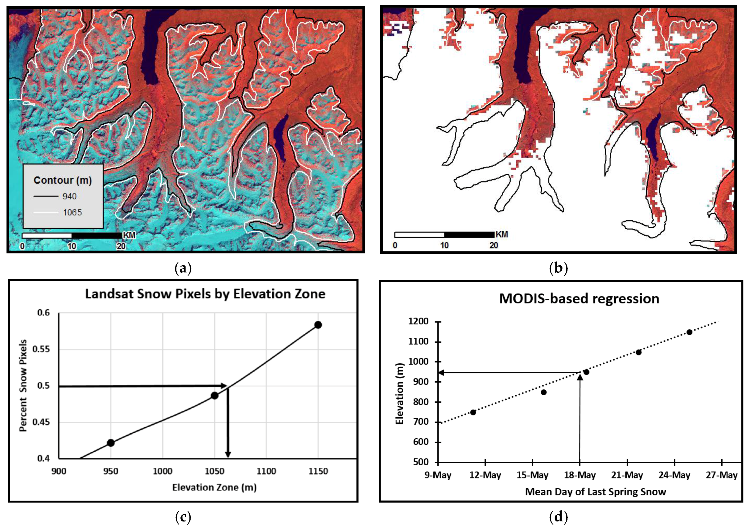
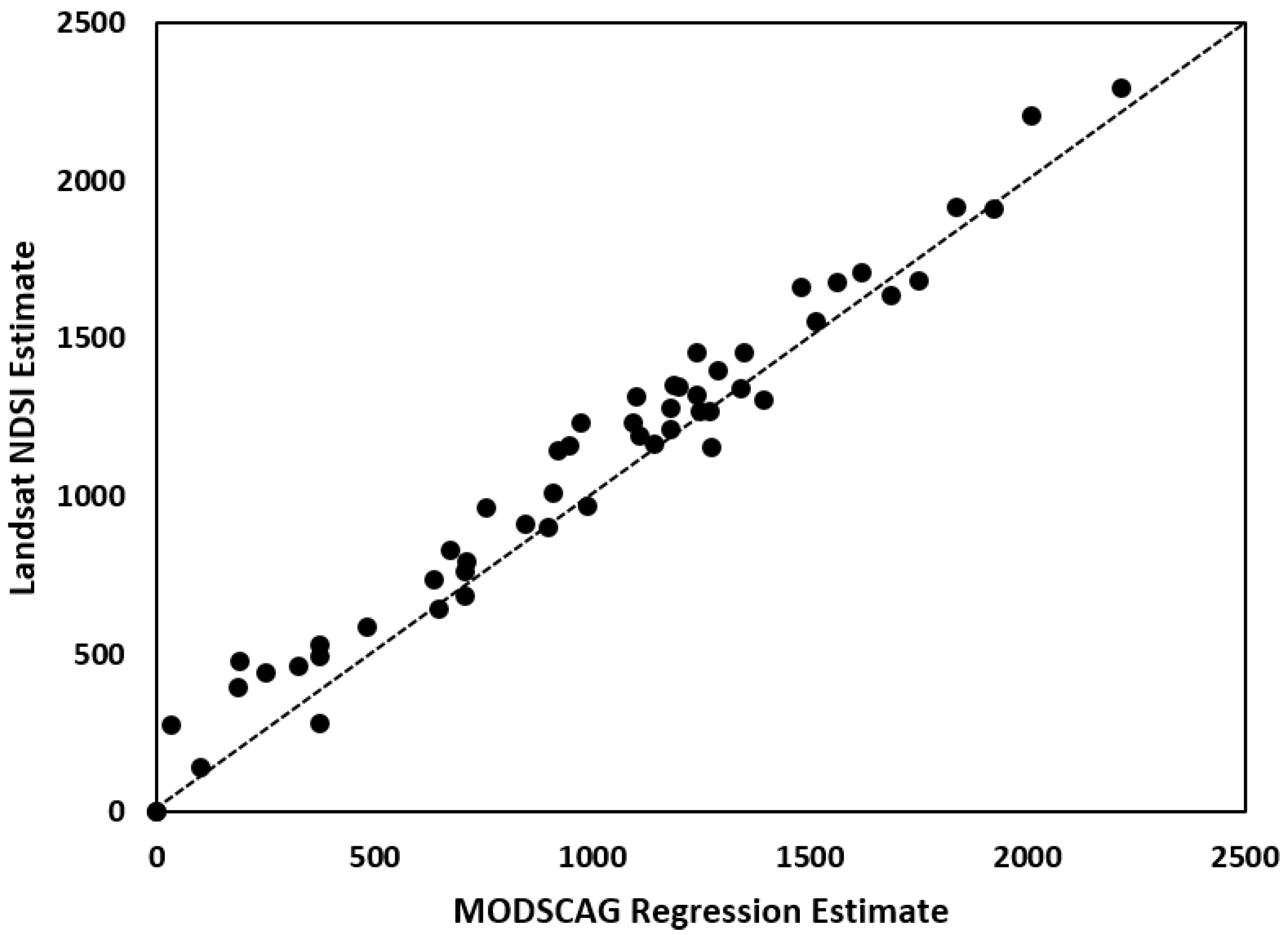
3.1. Comparison of Landsat NDSI and MODSCAG Based Snowline Elevation Estimates

Estimates of May snowline elevation from Landsat NDSI and MODSCAG regressions were similar (Figure 9), with a mean absolute error of 106 m (standard deviation of 77 m). The Landsat NDSI based snowline estimates were typically at higher elevation, perhaps due to the finer spatial resolution (30-m pixels for Landsat NDSI, 500-m pixels for MODSCAG) or due to the different methodological approaches. The uncertainty of elevation due to use of a regional elevation raster likely introduced error in both the MODSCAG regression and Landsat NDSI validation datasets. Also because of local conditions such as slope direction, topographic position, topographic control of wind-blown snow distribution, there is no contour elevation that perfectly matches snowline at a local scale (Figure 8a).

3.2. Mountain Area Climates

Based on the gridded climatic products, the 3 regional climatic classes were distinct. The Cold Arctic Mountain class always had a mean May temperature of less than 4.0 °C (as low as −0.1 °C). These mountains included all six areas of the Brooks Range in Alaska and the Richardson and Wernecke Mountains in northern Yukon. The other mountain areas had warmer mean May temperature; all above 4.5 °C and as high as 7.6 °C. The High Snowpack class always had a winter precipitation exceeding 300 mm, with a high of 936 mm. These were major glaciered mountains of Alaska including the south slopes of the central Alaska Range and Wrangell Mountains, the entire western Alaska Range and the Chugach, Talkeetna and Kenai Mountains. The Interior Mountains class had a winter precipitation less than 300 mm, with a low of 84 mm. These included most of the ranges in central Alaska and northwest Canada that were less influenced by Pacific Ocean storm flows. The warmest and driest area was the Tanana Uplands which is in interior Alaska, with mean May temperature of 7.0 °C and less than 85 mm of total winter precipitation.

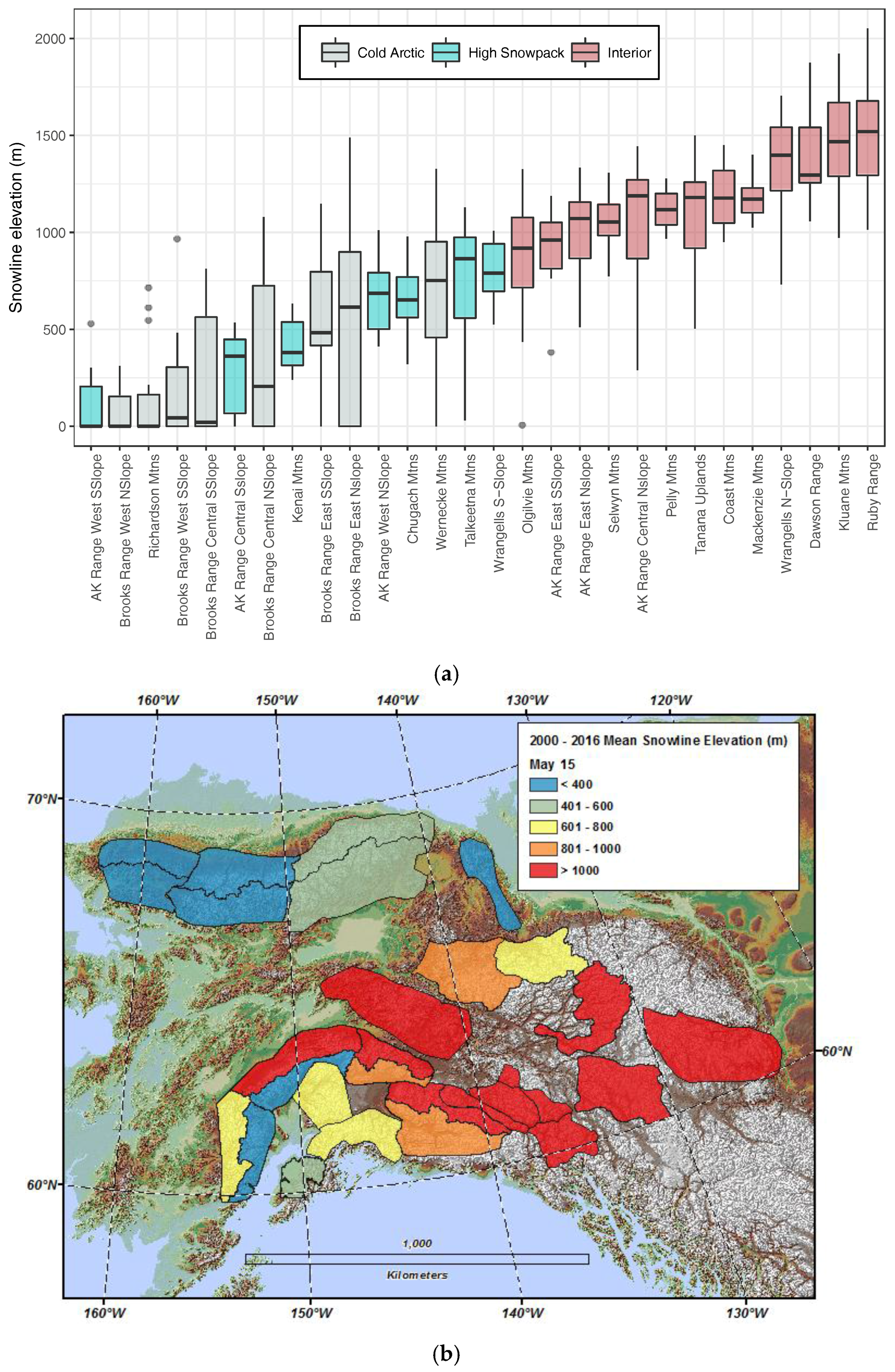
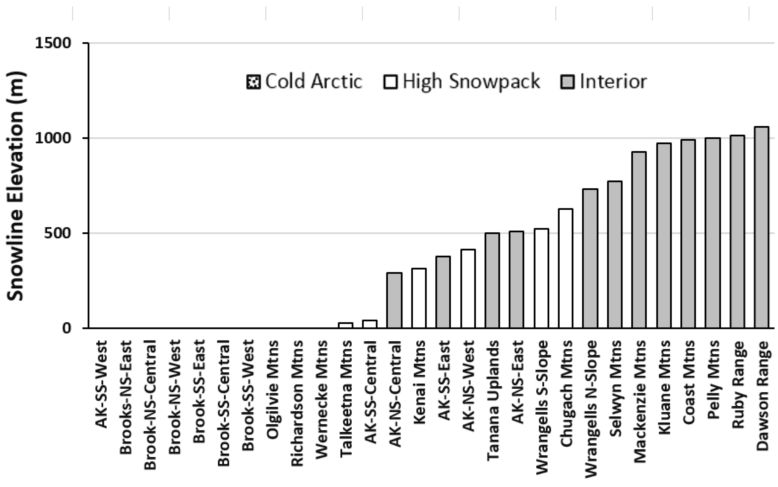
3.3. 2000–2016 Mean 15 May Snowline Elevation among Mountain Areas

Based on the daily MODSCAG snow fraction product, the mean 15 May 2000–2016 snowline elevation of snow line ranged from 0 to over 2000 m (Figure 10a) with the interior mountains class having the highest snowline elevation. Areas with mean 15 May snowline elevation less than 400 m were from cold arctic areas (Richardson Mountains, Brooks Range) or areas with high winter snow accumulation due to storm flow from the Pacific Ocean (Alaska Range central and western region, south slopes) (Figure 10b). The mean 2000–2016 snowline elevation was significantly related to mean May temperature and winter precipitation (Table 2).
Due to the influence of storms from the south, the snowline elevation was consistently lower on southerly slopes of the Alaska Range and Wrangell Mountains (Figure 11). In the Alaska Range, the difference in snowline elevation was least in eastern areas due to a west-to-east maritime to continental climate gradient.

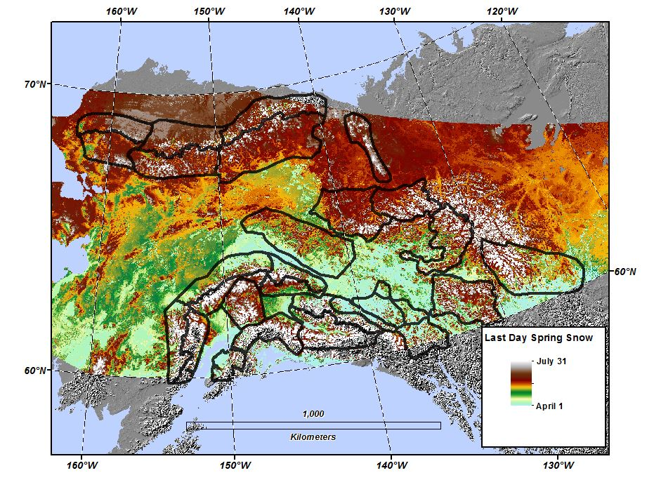
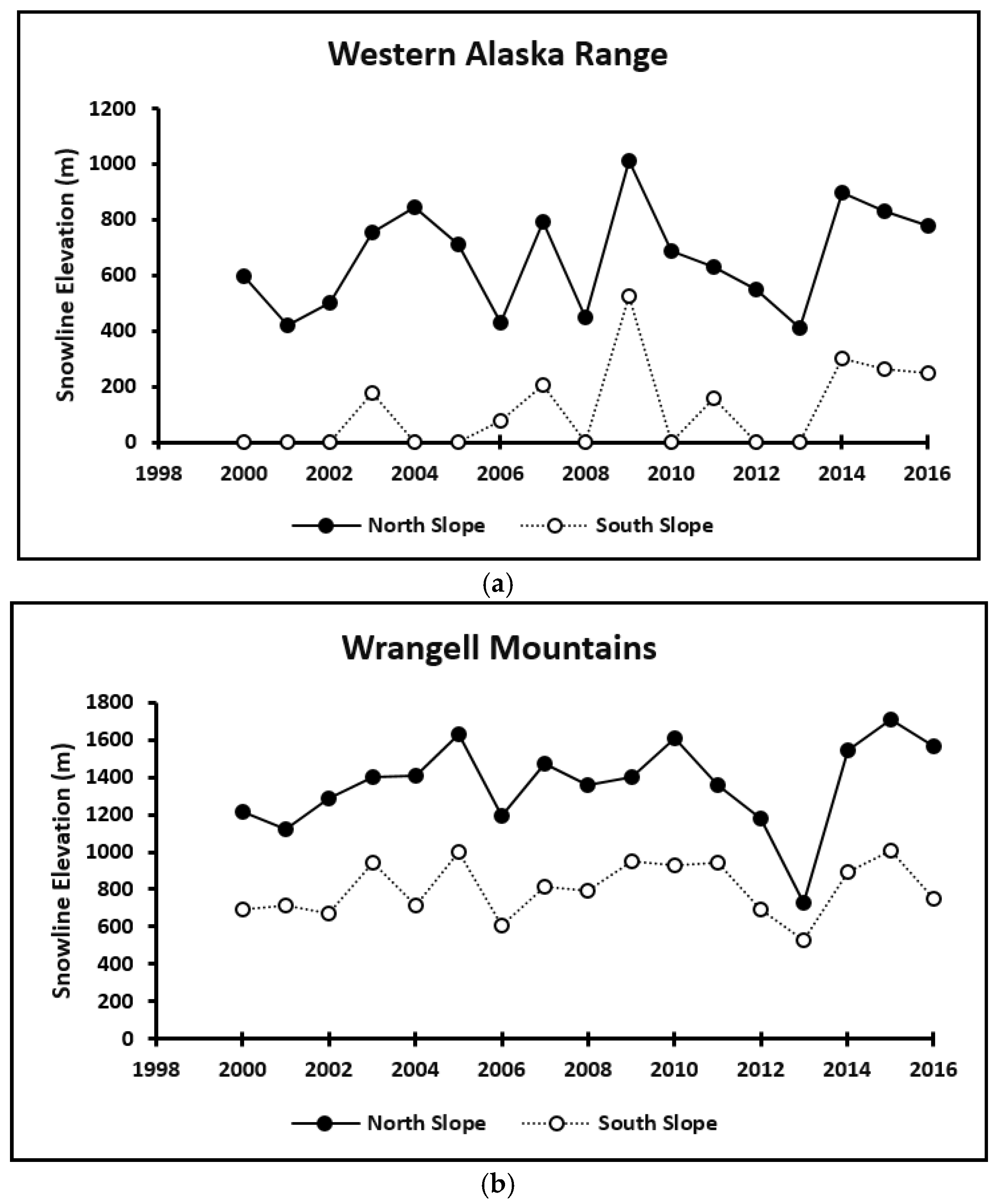
3.4. Spring 2013 Snowline Elevation among Mountain Areas

The late spring conditions of 2013 where the 15 May snow line elevation was less than 100 m, were primarily in the cold arctic mountain areas (Brooks Range, Richardson Mountains, Wernecke Mountains) and the high winter precipitation areas of the south slopes of the western and central Alaska Range (Figure 12). Eastern mountain areas with continental climate such as the north slope of the Wrangells and mountain ranges in southern Yukon had 15 May snowline elevations above 700 m.

4. Discussion

We developed a new application of the MODSCAG snow fraction product that accurately characterizes spatial and temporal regional variation in the elevation of spring snowline. We used Dall sheep as a case study because this alpine species is declining and thought to be sensitive to spring snow conditions [8]. However, the elevation of spring snowline is important for many alpine herbivores, because it affects access to forage as well as forage quality and quantity. New plant shoot growth typically begins after snowmelt and forage quality is highest in new plant growth because of high cell soluble content, which declines as plants matures and fiber accumulates [19]. In addition, nitrogen content of forage species typically declines with time after snowmelt [37,38]. Higher quality forage allows for shorter rumination time and thus more time to forage, the so-called multiplier effect [39]. Winter forage, or forage above snowline, is typically low quality: higher in fiber and lower in crude protein [40]. Thus if spring snowline elevation is relatively low, forage quantity and quality would be reduced relative to a warm spring when the snowline elevation is higher.
The variation among the 28 mountain areas was substantial in terms of decadal climate and elevation of spring snowline. For example, based on the gridded May temperature product, the cold arctic mountain areas had a mean May temperature of 1.9 °C, while the interior mountain areas had a mean May temperature of 6.1 °C. Based on the MODSCAG daily snow fraction product, the mean 15 May snowline elevation for the cold arctic mountain areas was 339 m, while the interior mountain areas had a mean 15 May snowline elevation of 1145 m. Variation in spring snow conditions can be substantial, for example in 2013 the 15 May elevation of snowline in the Chugach Mountains was above 500 m and lamb survival was high [41] relative to the Brooks Range areas where 15 May snowline elevation was 0 m and no lambs were observed in this region during 2013 lamb survey [42].
The magnitude of the observed inter-annual variability in spring snow conditions is especially relevant because the frequency and magnitude of climate extremes are expected to increase under climate change [43,44,45]. This increased variability may have stronger impacts on ecosystem functioning than gradually shifting means, because wildlife populations may be resilient to occasional extreme weather conditions but unable to persist if these conditions become more frequent [16]. For example, inter-annual variation in snowline was highest in the central and eastern Brooks Range areas (Figure 10a), which is the region experiencing the steepest decline in sheep populations and emergency harvest closures [42]. Dall sheep populations recover slowly from extreme weather events, since each adult ewe produces a maximum of one lamb per year [46]. Therefore, the effect of harsh years occurring at a higher frequency could be detrimental to their persistence.
How might spring snow conditions affect sheep populations? First, spring snow cover affects plant phenology, thus affecting nutrition for lactating ewes and hence lamb survival. For example, lambs born in early May experienced higher mortality rates, likely due to a low snowline restricting access to high-quality forage and increasing vulnerability to predators [47]. However, lambs born very late nurse from females feeding on forage of declining quality and post-weaned lambs have access to high quality forage for a shorter time. For example, delayed plant phenology during a late spring corresponded with a 2-week delay in onset of parturition and thus reduction in time available for lamb growth, weaning and acquisition of body reserves for ewes prior to the onset of plant senescence [48]. Second, foraging distance away from escape terrain may be greater due to a low snowline elevation, leading to greater risk of predation and less efficient foraging. For example, ewes foraged closer to escape terrain during a mild spring when forage was plentiful relative to a late spring when forage availability and quality was lower and ewes foraged less efficiently [11].
It is likely that sheep populations are more vulnerable to late spring conditions in the cold arctic mountain areas. For example, our regression estimates of 15 May snowline elevation were close to sea level for all cold arctic mountain areas in 2013. These ranges likely had low lamb recruitment in 2013. Although beyond the scope of this paper, our snowline elevation product can be combined with survey data to quantitatively assess the effects of spring snow conditions on alpine wildlife populations across broad regions. For example, we found that sheep recruitment declined with lower 15 May snowline elevations using a linear mixed model of 1570 Dall sheep aerial surveys and the effect increased with latitude [49].
Our focus was on May snowline because plant growth and high quality forage occurs at elevations just below melting snow. This application may also be useful for estimating the start of alpine plant growing season across the region, since new plant growth occurs below the snowline. True Further development of remotely sensed snow products will improve the ability of wildlife managers to anticipate and mitigate responses of wildlife to climate change.

5. Conclusions

To assess the inter-annual and regional variability of spring snowline elevation across 28 mountain areas in Alaska and northwestern Canada, we used a regression model approach with a daily regional remote sensing snow product. Due to frequent extensive cloud and cloud shadow cover in our study areas and a repeat orbit of 16-days, this type of regional assessment was not possible with Landsat sensor data. We found the 2000–2016 MODIS MODSCAG snow fraction product useful for this application and regression-based estimates of regional spring snowline elevation compared favorably with 5 May through 30 May snowline elevation estimates derived from Landsat-OLI scenes across Alaska and northwest Canada.

Acknowledgments

This research was supported by the NASA ABoVE program, Grants NNX15AV86A (DV), NNX15AU21A (LRP) and NNX15AU13A (AWN). We have funds for covering the costs to publish in open access. We thank Mark Melham and the anonymous reviewers for helping us improve the manuscript.

Author Contributions

David Verbyla processed the data, Troy Hegel delineated the mountain areas in western Canada and provided expertise about Dall sheep populations in Canada, Anne W. Nolin processed the daily MODSCAG tiles covering the study area, Madelon van de Kerk and Laura R. Prugh provided expertise about Dall sheep populations in Alaska, Thomas A. Kurkowski provided expertise about the gridded temperature and precipitation products. All authors collaborated to write the manuscript.

Conflicts of Interest

The authors declare no conflict of interest.

References

  1. Callaghan, T.V.; Johansson, M.; Brown, R.D.; Groisman, P.Y.; Labba, N.; Radionov, V.; Barry, R.G.; Bulygina, O.N.; Essery, R.L.H.; Frolov, D.M.; et al. The changing face of Arctic snow cover: A synthesis of observed and projected changes. AMBIO 2011, 40 (Suppl. 1), 17–31. [Google Scholar] [CrossRef]
  2. Ozgul, A.; Childs, D.Z.; Oli, M.K.; Armitage, K.B.; Blumstein, D.T.; Olson, L.E.; Tuljapurkar, S.; Coulson, T. Coupled dynamics of body mass and population growth in response to environmental change. Nature 2010, 466, 482–485. [Google Scholar] [CrossRef] [PubMed]
  3. Hegel, T.M.; Mysterud, A.; Huettmann, F.; Stenseth, N.C. Interacting effect of wolves and climate on recruitment in a northern mountain caribou population. Oikos 2010, 119, 1453–1461. [Google Scholar] [CrossRef]
  4. Adams, L.G. Marrow fat deposition and skeletal growth in caribou calves. J. Wildl. Manag. 2003, 67, 20–24. [Google Scholar] [CrossRef]
  5. Worley, K.; Strobeck, C.; Arthur, S.; Carey, J.; Schwantje, H.; Veitch, A.; Coltman, D.W. Population genetic structure of North American thinhorn sheep (Ovis dalli). Mol. Ecol. 2004, 13, 2545–2556. [Google Scholar] [CrossRef] [PubMed]
  6. Putkone, J.; Roe, G. Rain-on-snow events impact soil temperatures and affect ungulate survival. Geophys. Res. Lett. 2003, 30. [Google Scholar] [CrossRef]
  7. Pettorelli, N.; Pelletier, F.; von Hardenberg, A.; Festa-Bianchet, M.; Côté, S.D. Early onset of vegetation growth vs. rapid green-up: Impacts on juvenile mountain ungulates. Ecology 2007, 88, 381–390. [Google Scholar] [CrossRef] [PubMed]
  8. Alaska Department of Fish and Game. Trends in Alaska Sheep Populations, Hunting, and Harvests. Division of Wildlife Conservation, Wildlife Management Report 2014, ADFG/DWC/WMR-2014-3. Available online: https://www.adfg.alaska.gov/static/home/library/pdfs/wildlife/mgt_rpts/14_sheep_report_bog.pdf (accessed on 24 January 2017).
  9. Alaska Department of Fish and Game. Dall Sheep Management Report of Survey-Inventory Activities July 2007–June 2010, Project6.0, Harper, P. Editor. Available online: https://www.adfg.alaska.gov/static/home/library/pdfs/wildlife/mgt_rpts/11_sheep.pdf (accessed on 24 January 2017).
  10. Loehr, J.; Carey, J.; O’Hara, R.B.; Hik, D.S. The role of phenotypic plasticity in responses of hunted thinhorn sheep ram growth to changing climate conditions. J. Evol. Biol. 2010, 23, 783–790. [Google Scholar] [CrossRef] [PubMed]
  11. Rachlow, J.L.; Bowyer, R.T. Habitat selection by Dall’s sheep (Ovis dalli): Maternal trade-offs. J. Zool. 1998, 245, 457–465. [Google Scholar] [CrossRef]
  12. Arthur, S.M.; Prugh, L.R. Predator-mediated indirect effects of snowshoe hares on Dall’s sheep in Alaska. J. Wildl. Manag. 2010, 74, 1709–1721. [Google Scholar] [CrossRef]
  13. Stone, R.S.; Dutton, E.G.; Harris, J.M.; Longenecker, D. Earlier spring snowmelt in northern Alaska as an indicator of climate change. J. Geophys. Res. 2002, 107. [Google Scholar] [CrossRef]
  14. Brown, R.; Derksen, C.; Wang, L. A multi-data set analysis of variability and change in Arctic spring snow cover extent. J. Geophys. Res. 2010, 115, 1967–2008. [Google Scholar] [CrossRef]
  15. Šmejkalová, T.; Edwards, M.E.; Dash, J. Arctic lakes show strong decadal trend in earlier spring ice-out. Sci. Rep. 2016, 6, 38449. [Google Scholar] [CrossRef] [PubMed]
  16. Boyce, M.S.; Haridas, C.V.; Lee, C.T.; The NCEAS Stochastic Demography Working Group. Demography in an increasing variable world. Trends Ecol. Evol. 2006, 21, 141–148. [Google Scholar] [CrossRef] [PubMed]
  17. Price, M.F.; Byers, A.C.; Kohler, T.; Price, L.W. (Eds.) Mountain Geography: Physical and Human Dimensions; University of California Press: Los Angeles, CA, USA, 2013; p. 396. [Google Scholar]
  18. Shea, J.M.; Menounos, B.; Moore, R.D.; Tennant, C. An approach to derive regional snow lines and glacier mass change from MODIS imagery, Western North America. Cryosphere 2013, 7, 667–680. [Google Scholar] [CrossRef]
  19. Dedieu, J.-P.; Carlson, B.Z.; Bigot, S.; Sirguey, P.; Vionnet, V.; Choler, P. On the Importance of High-Resolution Time Series of Optical Imagery for Quantifying the Effects of Snow Cover Duration on Alpine Plant Habitat. Remote Sens. 2016, 8, 481. [Google Scholar] [CrossRef]
  20. Krajčí, P.; Holko, L.; Perdigão, R.A.; Parajka, J. Estimation of regional snowline elevation (RSLE) from MODIS images for seasonally snow covered mountain basins. J. Hydrol. 2014, 519, 1769–1778. [Google Scholar] [CrossRef]
  21. Hammond, T.; Yarie, J. Spatial prediction of climatic state factor regions in Alaska. Ecoscience 1996, 3, 490–501. [Google Scholar] [CrossRef]
  22. Stafford, J.M.; Wendler, G.; Curtis, J. Temperature and precipitation of Alaska: 50 year trend analysis. Theor. Appl. Climatol. 2000, 67, 33–44. [Google Scholar] [CrossRef]
  23. Fleming, M.D.; Chapin, F.S.; Cramer, W.; Hufford, G.L.; Serreze, M.C. Geographic patterns and dynamics of Alaskan climate interpolated from a sparse station record. Glob. Chang. Biol. 2000, 6, 49–58. [Google Scholar] [CrossRef]
  24. Olson, D.M.; Dinerstein, E.; Wikramanayake, E.D.; Burgess, N.D.; Powell, G.V.N.; Underwood, E.C.; D’Amico, J.A.; Itoua, I.; Strand, H.E.; Morrison, J.C.; et al. Terrestrial ecoregions of the world: A new map of life on Earth. Bioscience 2001, 51, 933–938. [Google Scholar] [CrossRef]
  25. Harris, I.; Jones, P.D.; Osborn, T.J.; Lister, D.H. Updated high-resolution grids of monthly climatic observations—the TS3.10 Dataset. Int. J. Climatol. 2014, 34, 62–642. [Google Scholar] [CrossRef] [Green Version]
  26. Scenario Networks for Alaska and Arctic Planning, University of Alaska. 2016. Available online: https://www.snap.uaf.edu/methods/downscaling (accessed on 24 January 2017).
  27. Hay, L.E.; Wilby, R.L.; Leavesley, G.H. A comparison of delta change and downscaled GCS scenarios for three mountain basins in the United States. J. Am. Water Res. Assoc. 2000, 35, 387–397. [Google Scholar] [CrossRef]
  28. Hayhoe, K.A. A Standardized Framework for Evaluating the Skill of Regional Climate Downscaled Techniques. Ph.D. Thesis, University of Illinois, Urbana, IL, USA, 2010. [Google Scholar]
  29. PRISM Climate Group, Oregon State University, Climate Normal Obtained. Available online: http://www.prism.oregonstate.edu (accessed on 24 January 2017).
  30. Daly, C.; Halbleib, M.; Smith, J.I.; Gibson, W.P.; Doggett, M.K.; Taylor, G.H.; Curtis, J.; Pasteris, P.P. Pysiographically sensitive mapping of climatological temperature and precipitation across the conterminous United States. Int. J. Climatol. 2008, 28, 2031–2064. [Google Scholar] [CrossRef]
  31. Simpson, J.J.; Hufford, G.L.; Daly, C.; Berg, J.S.; Fleming, M.D. Comparing maps of mean monthly surface temperature and precipitation for Alaska and adjacent areas of Canada produced by two different methods. Arctic 2005, 58, 137–161. [Google Scholar] [CrossRef]
  32. Dozier, J. Spectral signature of alpine snow cover from the Landsat Thematic Mapper. Remote Sens. Environ. 1989, 28, 9–22. [Google Scholar] [CrossRef]
  33. Painter, T.H.; Dozier, J.; Roberts, D.A.; Davis, R.E.; Green, R.O. Retrieval of subpixel snow-covered area and grain size from imaging spectrometer data. Remote Sens. Environ. 2003, 85, 64–77. [Google Scholar] [CrossRef]
  34. Painter, T.H.; Rittger, K.; McKenzie, C.; Slaughter, P.; Davis, R.E.; Dozier, J. Retrieval of subpixel snow covered area, grain size, and albedo from MODIS. Remote Sens. Environ. 2009, 113, 868–879. [Google Scholar] [CrossRef]
  35. Rittger, K.; Painter, T.H.; Dozier, J. Assessment of methods for mapping snow cover from MODIS. Adv. Water Res. 2013, 51, 367–380. [Google Scholar] [CrossRef]
  36. Raliegh, M.S.; Rittger, K.; Moore, C.E.; Henn, B.; Lutz, J.A.; Lundquist, J.D. Ground-based testing of MODIDS fractional snow cover in subalpine meadows and forests of the Sierra Nevada. Remote Sens. Environ. 2013, 128, 44–57. [Google Scholar] [CrossRef]
  37. Van Soest, P.J. Nutritional Ecology of the Ruminant; Cornell University Press: Corvallis, OR, USA, 1982; p. 374. [Google Scholar]
  38. Fox, J. Forage Quality of Carex macrochaeta Emerging from Alaskan Alpine Snowbanks through the Summer. Am. Midl. Nat. 1991, 126, 287–293. [Google Scholar] [CrossRef]
  39. White, R.G. Foraging patterns and their multiplier effects on productivity of northern ungulates. Oikos 1983, 40, 377–384. [Google Scholar] [CrossRef]
  40. Seip, D.R.; Bunnell, F.L. Nutrition of Stone’s sheep on burned and unburned rages. J. Wildl. Manag. 1985, 49, 397–405. [Google Scholar] [CrossRef]
  41. Lohuis, T. Ewe Dall Sheep Survival, Pregnancy and Partition Rates, and Lamb Recruitment in GMU 13D, Chugach Mountains, Alaska. Alaska Department of Fish and Game Annual Progress Report, AKW-4 Wildlife Restoration, FY2015, 10pp. Available online: https://www.adfg.alaska.gov/static/home/library/pdfs/wildlife/research_pdfs/6.16_10.pdf (accessed on 24 January 2017).
  42. Rattenbury, K.; Schmidt, J.; Phillips, L.; Arthur, S.; Borg, B.; Burch, J.; Joly, K.; Lawler, J.; Mangipane, B.; Putera, J. Recent trends in Dall’s sheep populations in Alaska’s National Parks and Preserves. In Proceedings of the Alaska Dall Sheep Working Group Meeting, Anchorage, AK, USA, 20–21 February 2016; Available online: https://www.adfg.alaska.gov/static/regulations/regprocess/gameboard/sheepcomm/pdfs/20160220/6nps.pdf (accessed on 24 January 2017).
  43. Nippert, J.B.; Knapp, A.K.; Briggs, J.M. Intra-annual rainfall variability and grassland productivity: Can the past predict the future? Plant Ecol. 2006, 184, 65–74. [Google Scholar] [CrossRef]
  44. Hansen, B.B.; Grøtan, V.; Aanes, R.; Sæther, B.-E.; Stien, A.; Fuglei, E.; Ims, R.A.; Yoccoz, N.G.; Pedersen, Å.Ø. Climate events synchronize the dynamics of a resident vertebrate community in the high arctic. Science 2013, 339, 313–315. [Google Scholar] [CrossRef] [PubMed]
  45. IPCC. Climate Change 2013: The Physical Science Basis. Contribution of Working Group I to the Fifth Assessment Report of the Intergovernmental Panel on Climate Change; Stocker, T.F., Qin, D., Plattner, G.-K., Tignor, M., Allen, S.K., Boschung, J., Nauels, A., Xia, Y., Bex, V., Midgley, P.M., Eds.; Cambridge University Press: Cambridge, UK, 2013. [Google Scholar]
  46. Hoefs, M. Twinning in Dall sheep. Can. Field-Nat. 1978, 92, 292–293. [Google Scholar]
  47. Bunnell, F.L. Factors controlling lambing period of Dall’s sheep. Can. J. Zool. 1980, 58, 1027–1031. [Google Scholar] [CrossRef] [PubMed]
  48. Rachlow, J.L.; Bowyer, R.T. Variability in maternal behavior by Dall’s Sheep: Environmental tracking or adaptive strategy. J. Mammal. 1994, 75, 323–337. [Google Scholar] [CrossRef]
  49. Van de Kerk, M.; Verbyla, D.; Nolin, A.W.; Sivy, K.J.; Prugh, L.R. Adverse effects of snow cover on Dall sheep populations increase with latitude. J. Biogeogr. 2016. submitted. [Google Scholar]
Figure 1. (a) Typical Dall sheep habitat from Wrangell Mountains, Alaska; (b) Dall sheep ewe and lamb (both photographs were from late August by D. Verbyla).
Remotesensing 09 01157 g001
Figure 2. Spring river ice-out dates observed from 1994–2016 at Nenana, interior Alaska (filled circles) and Dawson, Yukon (open circles). The 1994–2016 mean date of spring ice-out is show as dot-dashed line for Nenana and finer dashed line for Dawson. Sources: http://www.nenanaakiceclassic.com, http://yukonriverbreakup.com.
Remotesensing 09 01157 g002
Figure 3. Alpine climate classes based on regional climatology. (1) Cold arctic mountains in the Tundra biome; (2) High snowpack mountains in the Boreal biome influenced by southerly storm tracks from the Pacific Ocean; (3) Interior Mountains in the Boreal biome. Alpine areas included in this study: (1) Alaska Range East, South Slope; (2) Alaska Range East, North Slope; (3) Alaska Range Central, South Slope; (4) Alaska Range Central, North Slope; (5) Alaska Range West, South Slope; (6) Alaska Range West, North Slope; (7) Brooks Range East, South Slope; (8) Brooks Range East, North Slope; (9) Brooks Range Central, South Slope; (10) Brooks Range Central, North Slope; (11) Brooks Range West, South Slope; (12) Brooks Range West, North Slope; (13) Chugach Mountains; (14) Coast Mountains; (15) Dawson Range; (16) Kenai Mountains; (17) Kluane Mountains; (18) Mackenzie Mountains; (19) Olgilvie Mountains; (20) Pelly Mountains; (21) Richardson Mountains; (22) Ruby Range; (23) Selwyn Mountains; (24) Talkeetna Mountains; (25) Tanana Uplands; (26) Wernecke Mountains; (27) Wrangell Mountains North; (28) Wrangell Mountains South. Arrows portray major winter storm tracks from the Pacific Ocean.
Remotesensing 09 01157 g003
Figure 4. Last day of spring snow detected from daily MODSCAG data for 2016. Mountain areas are outlined as black polygons. The names of each mountain area are presented in Figure 1.
Remotesensing 09 01157 g004
Figure 5. Example of MODIS-based 2000–2016 regression trend lines predicting snowline elevation from mean day of last snow within each elevation zone, Chugach Mountain alpine area. The earliest (2009) and latest spring (2000) above 700 m are portrayed as thicker trend lines.
Remotesensing 09 01157 g005
Figure 6. Flowchart of geospatial methods used for each year (2000–2016).
Remotesensing 09 01157 g006
Figure 7. Thirty Landsat-8 OLI scenes used to validate MODSAG-based regression models.
Remotesensing 09 01157 g007
Figure 8. (a) Landsat OLI image from 18-May-2015 with 940 m and 1065-m contours; (b) MODSCAG snow/no snow classification for same date and area; (c) Snowline elevation estimated at 1065 m based on 18-May-2015 Landsat NDSI; (d) Snowline elevation estimated at 940 m based on 2015 MODSCAG last day of spring snow linear regression.
Remotesensing 09 01157 g008
Figure 9. Comparison of May snowline elevation estimates from Landsat NDSI and MODSCAG regressions (n = 53). These estimates were from May 2013, May 2014, May 2015 covering Alaska and Yukon mountain areas (Figure 7). Day of year ranged from 5 May through 30 May.
Remotesensing 09 01157 g009
Figure 10. (a) Box plots of estimated 15 May snowline elevations. The lower and upper hinges correspond to the first and third quartiles (the 25th and 75th percentiles). The horizontal line in the box represents the median. The upper/lower whisker lines extend from the hinge to the largest value no further than 1.5 * IQR from the hinge (where IQR is the inter-quartile range, or distance between the first and third quartiles); (b) 2000–2016 mean 15 May snowlines estimated from regressions.
Remotesensing 09 01157 g010
Figure 11. 2000–2016 snow line mean elevation on 15 May for north versus south-facing slopes within (a) western Alaska Range and (b) Wrangell Mountains. There was also a west-to-east maritime to continental climatic gradient along the Alaska Range.
Remotesensing 09 01157 g011
Figure 12. Modeled elevation of snow line on 15 May 2013 (Day of Year 135).
Remotesensing 09 01157 g012
Table 1. Characteristics of Dall Sheep mountain areas. See Section 2.2 for methods used to estimate May temperature and winter precipitation.
Mountain AreaArea km2Elevation Range (m)Mean May Temp. (°C)Total Winter Precip. (mm)Climatic Class
(1) Alaska Range East, South Slope12,177500–25005.2124Interior
(2) Alaska Range East, North Slope13,284300–25006.6112Interior
(3) Alaska Range Central, South Slope15,31450–25004.8442High Snowpack
(4) Alaska Range Central, North Slope28,124100–25006.7145Interior
(5) Alaska Range West, South Slope18,5830–25004.8936High Snowpack
(6) Alaska Range West, North Slope21,1810–25005.8458High Snowpack
(7) Brooks Range East, South Slope65,367200–24003.864Cold Arctic
(8) Brooks Range East, North Slope32,69850–25000.283Cold Arctic
(9) Brooks Range Central, South Slope33,79750–23002.0185Cold Arctic
(10) Brooks Range Central, North Slope31,667100–2200−0.1156Cold Arctic
(11) Brooks Range West, South Slope23,36750–15001.8248Cold Arctic
(12) Brooks Range West, North Slope20,311150–14000.1235Cold Arctic
(13) Chugach Mountains23,9370–25004.7807High Snowpack
(14) Coast Mountains18,688350–23505.8254Interior
(15) Dawson Range,9715600–20006.2113Interior
(16) Kenai Mountains11,3170–19007.6914High Snowpack
(17) Kluane Mountains9342500–25005.5112Interior
(18) Mackenzie Mountains60,535200–27005.8232Interior
(19) Olgilvie Mountains39,956200–22005.2125Interior
(20) Pelly Mountains39,118600–23005.7185Interior
(21) Richardson Mountains17,099150–17003.0161Interior
(22) Ruby Range14,256600–23006.4116Interior
(23) Selwyn Mountains33,511500–25005.9215Interior
(24) Talkeetna Mountains22,634100–25005.1326High Snowpack
(25) Tanana Uplands60,034150–19007.084Interior
(26) Wernecke Mountains27,722350–25004.0174Cold Arctic
(27) Wrangell Mountains, North Slope18,895500–25006.6100Interior
(28) Wrangell Mountains, South Slope32,99450–25006.3480High Snowpack
Table 2. Regression model predicting mean 2000–2016 snowline elevation as a function of 2000–2009 decadal mean May temperature and mean total winter precipitation (p < 0.001, R2 = 0.71, n = 28).
CoefficientStd. Errorp-Value
Intercept337.96117.530.00812
May temperature (°C)148.3622.032<0.0001
Winter Precip (mm)−0.98370.1934<0.0001

