Sparse Unmixing of Hyperspectral Data with Noise Level Estimation


1
Electronic Information School, Wuhan University, Wuhan 430072, China
2
School of Electronic Information and Communications, Huazhong University of Science and Technology, Wuhan 430074, China
3
School of Mathematics and Computer Science, Wuhan Polytechnic University, Wuhan 430023, China
*
Authors to whom correspondence should be addressed.
Remote Sens. 2017, 9(11), 1166; https://doi.org/10.3390/rs9111166
Submission received: 5 October 2017
/
Revised: 4 November 2017
/
Accepted: 10 November 2017
/
Published: 13 November 2017
(This article belongs to the Section Remote Sensing Image Processing)
Abstract
:Recently, sparse unmixing has received particular attention in the analysis of hyperspectral images (HSIs). However, traditional sparse unmixing ignores the different noise levels in different bands of HSIs, making such methods sensitive to different noise levels. To overcome this problem, the noise levels at different bands are assumed to be different in this paper, and a general sparse unmixing method based on noise level estimation (SU-NLE) under the sparse regression framework is proposed. First, the noise in each band is estimated on the basis of the multiple regression theory in hyperspectral applications, given that neighboring spectral bands are usually highly correlated. Second, the noise weighting matrix can be obtained from the estimated noise. Third, the noise weighting matrix is integrated into the sparse regression unmixing framework, which can alleviate the impact of different noise levels at different bands. Finally, the proposed SU-NLE is solved by the alternative direction method of multipliers. Experiments on synthetic datasets show that the signal-to-reconstruction error of the proposed SU-NLE is considerably higher than those of the corresponding traditional sparse regression unmixing methods without noise level estimation, which demonstrates the efficiency of integrating noise level estimation into the sparse regression unmixing framework. The proposed SU-NLE also shows promising results in real HSIs.
1. Introduction
Hyperspectral imaging has been a widely used commodity, and hyperspectral image (HSI) is intrinsically a data cube which has two spatial dimensions (width and height) and a spectral dimension. The wealth of spectral information in HSIs has opened new perspectives in different applications, such as target detection, spectral unmixing, object classification, and matching [1,2,3,4,5,6,7,8,9,10,11,12,13]. The underlying assumption in object classification techniques is that each pixel comprises the response of only one material. Mixed pixels are prevalent in HSIs due to the insufficient spatial resolution of imaging sensors and the mixing effects of ground surface, which make several different materials jointly occupy a single pixel, thereby resulting in great difficulties for the accurate interpretation of HSIs [14,15]. Therefore, spectral unmixing is essential as it aims at decomposing mixed pixels into a collection of pure spectral signatures, called endmembers, and their corresponding proportions in each pixel, called abundances [16,17].
To address this problem, linear mixing model (LMM) has been extensively applied in the fields of geoscience and remote sensing processing due to its relative simplicity and straightforward interpretation [15]. Spectral unmixing can be roughly divided into three main classes according to the prior knowledge of the endmembers [18], namely, supervised, unsupervised, and semi-supervised methods. Supervised unmixing methods estimate the abundances with known endmembers, and the most representative supervised unmixing method is the fully constrained least squares method [19]. Unsupervised unmixing methods aim to estimate both the endmembers and their corresponding abundances. One approach is to extract the endmember using endmember extraction algorithms [20,21] first, and then their corresponding abundances can be estimated by supervised unmixing methods. In addition, the endmembers and their corresponding abundances can be estimated simultaneously by independent component analysis methods [22,23] and non-negative matrix factorization-based methods [24,25,26]. A semi-supervised unmixing method assumes that a mixed pixel can be formulated in the form of linear combinations of numerous pure spectral signatures (library) known in advance and then finds the optimal subset of signatures to optimally model the mixed pixel in the scene, which leads to a sparse solution [27].
Sparse representation has recently been studied in a variety of problems [28,29,30]. Sparse unmixing is a semi-supervised unmixing method, which assumes that the observed HSI can be formulated to find the optimal subset of pure spectral signatures from a prior large spectral library. Some greedy algorithms have been proposed for sparse unmixing of HSI, such as the orthogonal matching pursuit (OMP), OMP and the iterative spectral mixture analysis (ISMA) algorithm. However, the unmixing accuracies of these algorithms decrease rapidly due to the high correlation of the spectra of different materials. To overcome this problem, Akhtar et al. proposed a novel futuristic heuristic greedy algorithm called OMP-Star [31], which does not only show robustness against the high correlation among the spectra but also exhibits the advantages of greedy algorithms. Tang et al. proposed the regularized simultaneous forward-backward greedy algorithm (RSFoBa) [32] for the sparse unmixing of HSIs and revealed that the combination of the forward and backward greedy steps can make the RSFoBa more stable and less likely trapped into the local optimum than traditional greedy algorithms. Shi et al. proposed a novel sparse unmixing algorithm called subspace matching pursuit [33], which exploits the fact that the pixels in the HSI are usually highly correlated; thus, they utilized the low-degree mixed pixels in the HSI to iteratively find a subspace for reconstructing the HSI. Fu et al. proposed a new self-dictionary multiple measurement vector (SD-MMV) model [34], where the measured hyperspectral pixels are adopted as the dictionary, and then a greedy SD-MMV algorithm using simultaneous orthogonal matching pursuit is proposed.
In addition, taking advantage of sparse optimization, several sparse regression-based unmixing methods that have anti-noise capability have also been proposed [35]. Bioucas et al. proposed a sparse unmixing method through variable splitting and augmented Lagrangian (SUnSAL) [36], which formulated the sparse unmixing method as a sparse regression problem, and the sparsity of abundances was characterized by the norm. However, the norm leads to inconsistent endmember selection. To address this problem, Themelis et al. proposed the weighted lasso sparse unmixing method [18], where weights are adopted to penalize different coefficients in the regularization scheme. SUnSAL also ignores the spatial information in HSIs. To maximize the spatial information in HSIs, Iordache et al. included the total variation regularization term to the SUnSAL and developed a new sparse unmixing algorithm called SUnSAL and total variation [37]. Mei et al. proposed a novel spatially and spectrally constrained sparse unmixing algorithm by imposing spatial and spectral constraints in selecting endmembers from a spectral library that consists of image-derived endmembers [38], which can alleviate the influence of spectral variation. Zhong et al. proposed a new sparse unmixing algorithm based on non-local means (NLSU) [39], and it introduces a non-local mean regularization term for sparse unmixing through a weighting average for all the pixels in the abundance image, which is adopted to exploit the similar patterns and structures of the abundance. Iordache et al. also proposed collaborative SUnSAL (CLSUnSAL) to improve unmixing results by adopting the collaborative sparse regression framework [40], where the sparsity of abundance is characterized by the norm and simultaneously imposed on all pixels in the HSI. Zheng et al. proposed a new weighted sparse regression unmixing method [41], where the weights adopted for the next iteration are computed from the value of the current solution. To overcome the difficulty in selecting the regularization parameter, Feng et al. proposed the adaptive spatial regularization sparse unmixing method based on the maximum a posteriori estimation [42]. To improve the unmixing performance on noisy HSIs Zhang et al. proposed framelet-based sparse unmixing, which can promote the sparsity of abundance in the framelet domain and discriminate the approximation and detail components of HSI after framelet decomposition [35]. To consider the possible nonlinear effects, two novel sparse unmixing methods have been proposed [43,44]. Considering that norm has shown numerous advantages over norm, sparse unmixing methods based on norm have also been developed [45,46]. Salehani et al. developed a new sparse unmixing method using arctan smoothing [14], which starts from an norm optimization problem and iteratively converges quickly to an norm optimization problem.
Other types of sparse unmixing methods have also been proposed. Themelis et al. presented a novel hierarchical Bayesian method for the sparse unmixing of HSIs [47] and selected suitable priors to ensure the non-negativity of the abundances and favor sparse solutions for the abundances. Given that the relaxation to the original norm may introduce sensitive weighted parameters and additional calculation error, Xu et al. thus developed a novel sparse unmixing method based on multi-objective optimization without any relaxation [48] that contains two correlative objectives: minimizing the reconstruction error and controlling the sparsity of abundance. The priori knowledge of HSIs has been integrated into the framework of hyperspectral unmixing. In addition, Tang et al. proposed a novel method called sparse unmixing using spectra as a priori information [49], which can address the generation of virtual endmembers and the absence of pure pixels.
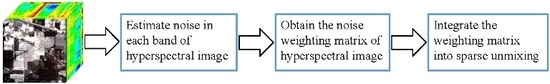
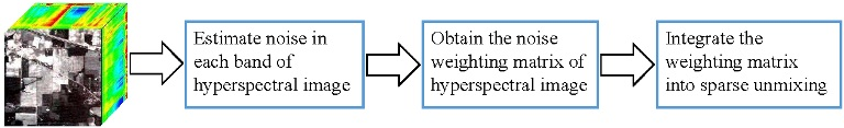
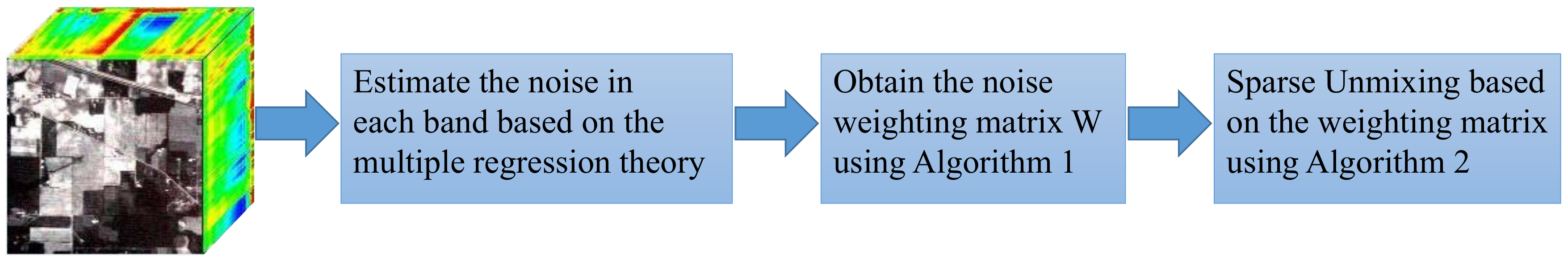
However, all these methods ignore the different noise levels in different bands of HSIs, and thus sensitive to the different noise levels. To make the unmixing peformance robust for outlier and noise, some methods based on correntropy have been proposed [50,51]. Specifically, Zhu et al. [51] proposed a sparsity-promoting correntropy-based unmixing method named CUSAL-SP and has shown promising performance. Figure 1 shows five representative bands of the Indian Pines image. As shown in Figure 1, the noise levels of the five representative bands are different. In addition, the noise levels of Bands 1 and 220 are evidently higher than those of the other three bands, and previous sparse unmixing methods treat all the bands similarly. However, for real HSIs, the noise levels of different bands vary, and bands with high noise levels will dominate the loss function , where denotes the collected mixed pixel, denotes the spectral library, denotes the abundance matrix, and represents the matrix Frobenius norm. The estimation of the abundance of small noise level would be severely affected and deviate significantly from the true value. Thus, treating all bands in the same way would be inaccurate. To overcome this problem, according to Figure 1, the noise levels at different bands are assumed to be different in this paper, and a novel sparse unmixing method based on noise level estimation (SU-NLE) is proposed, where the algorithm flow of the proposed method is presented in Figure 2. First, a simple and efficient noise estimation method based on the multiple regression theory developed by Bioucas and Nascimento [52] is adopted to estimate the noise in each band of HSI. Second, to consider the noise level of each band, the proposed SU-NLE adopts a weighting strategy for treating all bands separately, that is, the higher the noise level is, the smaller the weight of the band is. The weighting strategy can strike a balance between different noise levels in different bands of the HSI, thereby alleviating the impact of the noise levels at different bands on the final sparse unmixing accuracy. Third, the noise weighting matrix obtained is integrated into the sparse regression unmixing framework, which can make the proposed SU-NLE robust for different noise levels in different bands. Finally, to solve the proposed SU-NLE, we adopt the alternative direction method of multipliers (ADMM), which is a simple and powerful algorithm that is suitable for constrained optimization.
The main contribution of this work is the general sparse unmixing method called SU-NLE, which adopts a simple and efficient weighting strategy to strike a balance between different noise levels in different HSI bands, and the weighting strategy is integrated into the sparse regression unmixing framework to formulate the proposed method. When the noise level of each band is the same, the weighting matrix is the identity matrix, and it is reduced to traditional sparse regression methods. Thus, the proposed SU-NLE is more general and adaptive. The proposed SU-NLE can be solved by the ADMM. Experiments on synthetic datasets show that the signal-to-reconstruction error (SRE) of the proposed SU-NLE is considerably higher than those of the corresponding traditional sparse regression unmixing methods without noise level estimation, which demonstrates the efficiency of integrating noise level estimation into the sparse regression unmixing framework. The proposed SU-NLE also shows promising results in real HSIs.
The remainder of this paper is organized as follows. In Section 2, we describe the proposed SU-NLE and discuss the ADMM developed for solving the proposed method. In Section 3, we evaluate the performances of the proposed SU-NLE and other algorithms on synthetic datasets and real HSIs. Section 4 concludes this paper.
2. Sparse Unmixing of HSI with Noise Level Estimation
In this section, we will describe the proposed sparse unmixing method SU-NLE. Then, we will develop an ADMM for solving the proposed method. Finally, we will describe the relation of our proposed SU-NLE with traditional sparse regression unmixing methods.
2.1. The Proposed SU-NLE
The LMM is widely admitted in the analysis of HSI, which assumes that a pixel can be represented as a linear combination of endmembers, and the linear coefficients are their corresponding abundances. Mathematically, the LMM can be written as follows:
where denotes a vector of observed pixel in HSI, with D denoting the number of bands, and denotes the endmember, with M denoting the number of endmembers, denotes the abundance vector, and denotes the additive noise. Thus, the matrix formulation of LMM can be written as follows:
where denotes the collected mixtures matrix, with P denoting the number of pixels, denotes the abundance matrix, and the collected additive noise.
The abundances have to obey two constraints, namely, they have to be nonnegative (ANC), and they should sum to 1 (ASC), i.e.,
However, for the unmixing of HSI in practice, the ASC constraint not always holds true due to the intensive signature variability in an HSI [27]. Thus, we ignore the ASC constraint in unmixing of HSI.
Although the traditional sparse regression unmixing methods have been widely used in sparse unmixing of HSI, they do not take the noise level of different bands into consideration. As can be clearly seen from Figure 1, the noise level of the five representative bands is different, and the noise levels of bands 1 and 220 are obviously higher than those of the other three bands. Besides, the previous works correlated with noise estimation of HSI [52,53,54] have demonstrated that the hyperspectral imaging spectrometers adopt very narrow band, which makes the energy acquired in each band not enough to obtain high signal-to-noise ratio (SNR), and the HSI is usually corrupted by wavelength-dependent and sensor-specific noise, which not only degrades the visual quality of the HSI but also limits the precision of the subsequent image interpretation and analysis. That is to say, the noise of HSI is wavelength-dependent, thus the noise levels of different bands are different. However, the traditional sparse regression unmixing methods treat all the bands in the same way, which do not take the different noise levels of different bands into consideration. These bands having high level of noise will dominate the loss function , and the estimation of the whole abundance matrix would be seriously affected, which makes it deviate far away from the true value. Thus, it would be inappropriate to treat all the bands in the same way.
To overcome the above mentioned problem, according to the Figure 1 and the previous works correlated with noise estimation of HSI [52,53,54], it is natural to assume that the noise levels at different bands are different. We adopt a simple and efficient noise estimation method based on the multiple regression theory, developed by Bioucas and Nascimento [52], to estimate the noise in each band of HSI. The underlying reason is that the neighboring spectral bands are usually highly correlated, which makes the multiple regression theory well suited for noise estimation of HSI.
Define the , and , where denotes the ith column of , i.e., denotes all the pixels of ith band of HSI. It is assumed in [52] that is a linear combination of the remaining bands. Mathematically, it can be written as follows:
where is the regression vector, and is the modeling error vector. can be estimated based on the least squares regression scheme for each band:
Then, the estimated noise in each band of HSI is as follows:
Thus, it is natural to estimate the noise level of each band as follows:
where denotes the level of noise in each band, and denotes the jth pixel of ith band of HSI.
After calculating the noise level in each band, we adopt a simple and effective weighting strategy to strike a balance between different noise levels in different bands of HSI, and higher noise level band would have smaller weight. The diagonal element of the weighting matrix is the reciprocal of the noise level in each band, and the non-diagonal elements are all zero, which can alleviate the timpact of the noise levels at different bands. Mathematically, the diagonal element of the weighting matrix is as follows:
where denotes the weighting matrix. To sum up, the detailed procedure to obtain the weighting matrix is listed in Algorithm 1.
| Algorithm 1: Obtain the weighting matrix |
 |
After obtaining the weighting matrix, we integrate the weighting matrix into the sparse regression unmixing framework to formulate our proposed method. Sparse unmixing is a semi-supervised unmixing method, which assumes that the observed HSI can be formulated as finding the optimal subset of pure spectral signatures from a prior large spectral library. In other words, hyperspectral vectors are approximated by a linear combination of a “small” number of spectral signatures in the library, and it is widely admitted that the sparsity of abundance can be characterized by the norm. To take the noise level and the sparsity of abundance into account, mathematically, it can be written as follows:
where is a regularization parameter, which strikes the balance between the quadratic data fidelity term and the sparsity-inducing regularization term.
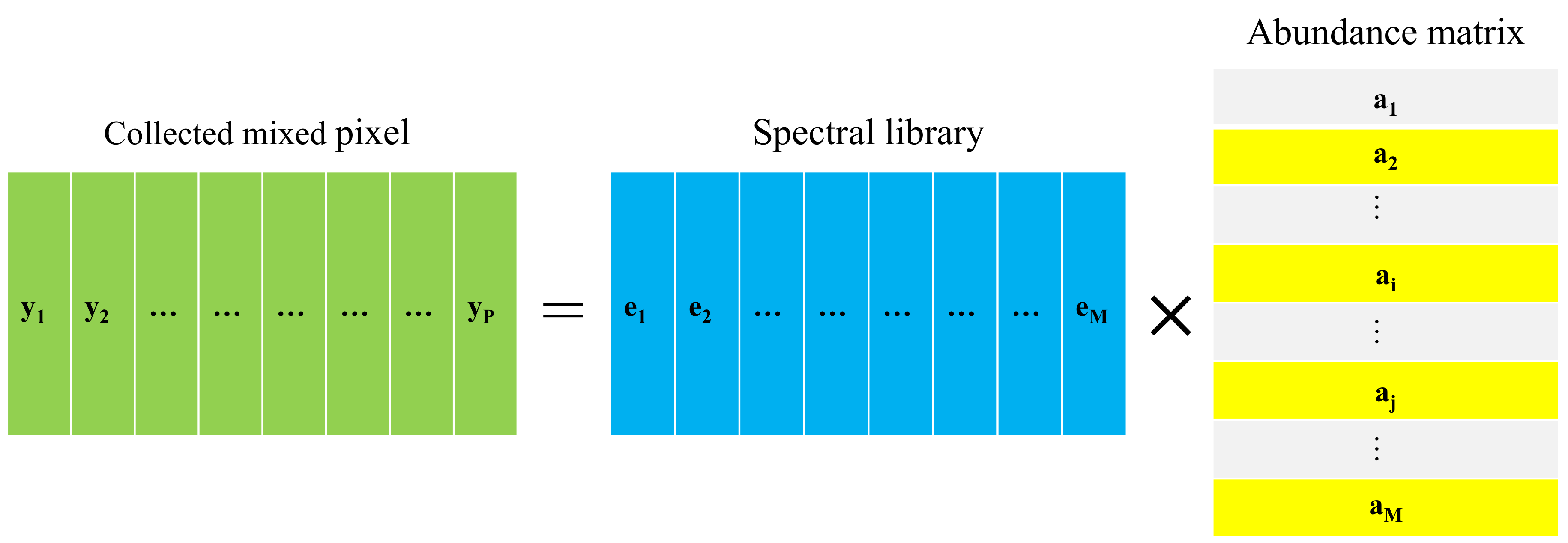
However, mutual coherence of the endmember signatures in spectral library is usually very high. Previous work in [27] has demonstrated that the mutual coherence has a large impact on the final sparse unmixing solutions. The more similar the endmember signatures in spectral library are, the more difficult the sparse unmixing is. To overcome the above mentioned problems, Iordache et al. proposed the collaborative SUnSAL (CLSUnSAL) to improve the unmixing results by adopting the collaborative sparse regression framework [40]. Figure 3 shows the graphical illustration of the CLSUnSAL, and it can be clearly seen from Figure 3 that the nonzero abundance should appear in only a few lines, which indicates sparsity along the pixels of an HSI. In [55], it has been demonstrated that the probability of sparse collaborative recovery failure decays exponentially with regard to the number of channels, which demonstrates that multichannel sparse recovery is better than single channel methods. In addition, the probability bounds still hold true even for a small number of signals. In other words, for a real HSI, the collaborative (also called “simultaneous” or “multitask”) sparse regression approach has shown advantages over the noncollaborative ones, which leads to a structured solution since the fractional abundances contain only a few nonzero lines along the pixels of an HSI [40]. So it can be assumed that the abundance has the underlying collaborative sparse property, which is characterized by the norm. Therefore, to take the noise level and the collaborative sparsity of abundance into account, mathematically, it can be written as follows:
where for the abundance matrix , norm is defined as follows:
The norm can impose sparsity among the endmembers simultaneously (collaboratively) for all pixels, which enforces the presence of the same singletons in the image pixels. The main difference between using norm and norm is that the former adopts the pixel-wise independent regression, while the latter imposes sparsity among all the pixels collaboratively [56].
Therefore, for our proposed SU-NLE, mathematically, it can be written as follows:
For the data fidelity term, the weighting matrix is used to strike a balance between different noise levels in different bands of HSI, and the regularization term is used to impose sparsity of HSI, where d = 1 or 2. When d = 1, the reduces to , and the Equation (12) reduces to Equation (10), thus Equation (10) is named as SU-NLE (d = 1). When d = 2, the reduces to , and the Equation (12) reduces to Equation (11), thus Equation (11) is named as SU-NLE (d = 2).
2.2. ADMM for Solving SU-NLE
To solve the optimization problem in Equation (12), we develop an ADMM to take advantage of the problem structure [57]. By adding the auxiliary matrix and , the problem in Equation (12) can be reformulated as follows:
where is the indicator function for the nonnegative orthant , represents the -th component of , and is zero if belongs to the nonnegative orthant, and otherwise.
By using the compact form, Equation (13) can be rewritten as follows:
where , , , , , . Thus, the augmented Lagrangian function can be formed as follows:
where is a positive constant, is a scaled dual variable, and represents the Lagrange multipliers. Therefore, we can sequentially optimizes with respect to , and .
To update , when d = 1, we solve
where denotes the shrinkage operator [58], and is a threshold parameter.
When d = 2, we solve
whose solution is the well-known vect-soft threshold [59], applied independently to each row r of the update variable as follows:
where , and vect-soft(b, ) denotes the row-wise application of the vect-soft-threshold function .
To update , we solve
To update , we solve
Thus, the primal and dual residuals and are as follows:
According to [57], the stopping criterion is as follows:
In the ADMM scheme for solving RSU, has a strong influence on the final convergence speed. We use the same approach as in [57] to update , which aims at keeping the ratio between the ADMM primal norms and dual residual norms within a given positive interval, and they both converge to zero.
Proposition 1.
The function g in Equation (14) is closed, proper, and convex. If there exists a solution and , then the sequences and converge to and , respectively. Otherwise, one of the sequences and diverges [57].
According to [57], we can obtain the Proposition 1, and the detailed proof of the convergence can be referred to [57]. To sum up, the detailed procedure for solving the Equation (12) is listed in Algorithm 2.
| Algorithm 2: Solving Equation (12) with ADMM |
 |
2.3. Relation to Traditional Sparse Regression Unmixing Methods
For the convenience of comparison, we adopt a simple preprocessing method for the weighting matrix, i.e., the diagonal elements of weighting matrix all divide by their mean values, since the diagonal elements of weighting matrix of the proposed SU-NLE are usually very large, which usually have two orders of magnitude. Our SU-NLE can take different levels of noise of different bands into account. Besides, when the noise level of each band is the same, the weighting matrix is the identity matrix, when d = 1, the reduces to , thus the proposed SU-NLE reduces to SUnSAL [36] when the noise level of each band is the same and d = 1. When d = 2, the reduces to , thus the proposed SU-NLE reduces to CLSUnSAL [40] when the noise level of each band is the same and d = 2. So the proposed SU-NLE is more general and adaptive than traditional sparse regression unmixing methods.
3. Experiments
In this section, we will evaluate the performances of the proposed SU-NLE and the compared algorithms both on the synthetic datasets and real HSIs. To demonstrate the efficiency of the proposed SU-NLE, we mainly compare with three strongly correlated algorithms, i.e., SUnSAL [36], CLSUnSAL [40] and CUSAL-SP [51]. To evaluate the performance of different sparse unmixing algorithms, we adopt the SRE [27] to measure the power between the signal and error, and the SRE is defined as follows:
where and denotes the actual and estimated abundance, respectively. Generally speaking, larger SRE means better hyperspectral sparse unmixing performance.
3.1. Experimental Results with Synthetic Data
In the synthetic data experiments, the spectral library that we use is a dictionary of minerals from the United States Geological Survey (USGS) digital spectral library available at http://speclab.cr.usgs.gov/spectral-lib.html, which has 224 spectral bands uniformly ranging from 0.4 m to 2.5 m. The adopted spectral library in this paper has 240 endmembers, which have been previous used in [14,40]. Besides, we have conducted a lot of tests to find an appropriate parameter setting for the proposed SU-NLE and the other compared algorithms. The regularization parameter plays an important role in the regression based sparse unmixing algorithms, which controls the trade-off between the fidelity term and the sparsity of the abundance. The Lagrange multiplier regularization parameter , the error tolerance and the maximum number of iterations, which have less impact on the unmixing accuracy of the regression based sparse unmixing algorithms, are set to a fixed value. Therefore, the common parameter setting of the methods SU-NLE, SUnSAL and CLSUnSAL for synthetic data is shown in Table 1. We also conduct experiments on the simulated experiment I using CUSAL-SP [51] for {, , , , , 1, , , , , }, and the experiments are performed on a server with 3.1-GHz Intel Core CPU, 16-GB memory, and Matlab code. The time consumption of CUSAL-SP is less than s when . However, the time consumption of CUSAL-SP is more than 12 h when . If we tune the regularization parameter of CUSAL-SP in the same way as SUnSAl, CLSUnSAL and the proposed SU-NLE, the time consumption of all the simulated experiments would be more than one year. Nevertheless, we tune the regularization parameter of CUSAL-SP according to [1]. Specifically, the sparsity-promoting parameter is tuned using the set , is a rough measure of the sparsity level of the unknown abundance matrix from the collected mixtures matrix according to [60]. The is usually ranging from 0 to 1, so is less than , and the time consumption of CUSAL-SP is comparable with SUnSAl, CLSUnSAL and the proposed SU-NLE. Since the way to tune the regularization parameter of CUSAL-SP and other methods is different, so we do not show the SRE results of CUSAL-SP with respect to different . Therefore, we tune the sparse unmixing performance of SUnSAL, CLSUnSAL and the proposed SU-NLE using {, , , , , 1, , , , , }, and tune the sparse unmixing performance of CUSAL-SP using .
3.1.1. Simulated experiment I
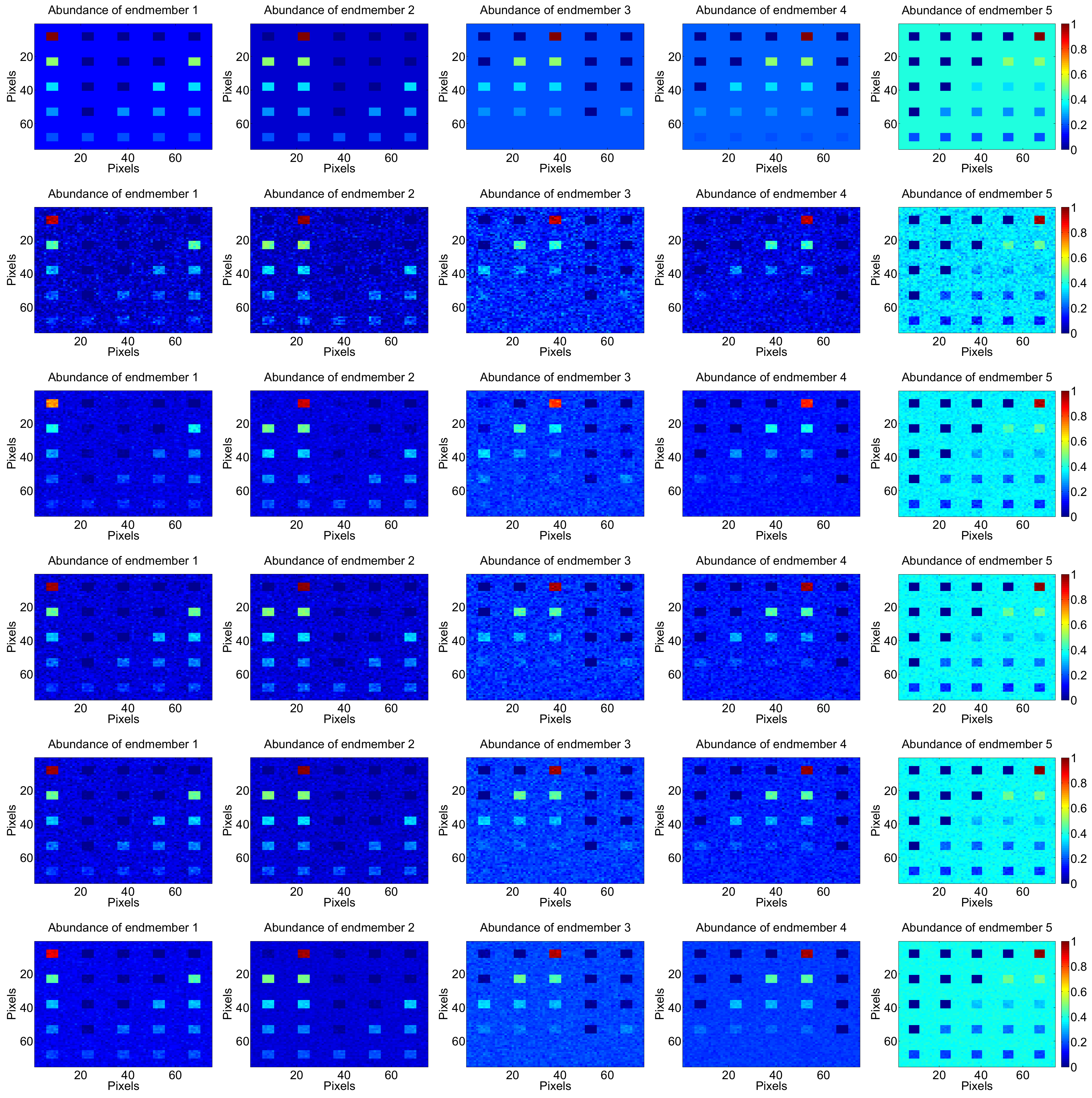
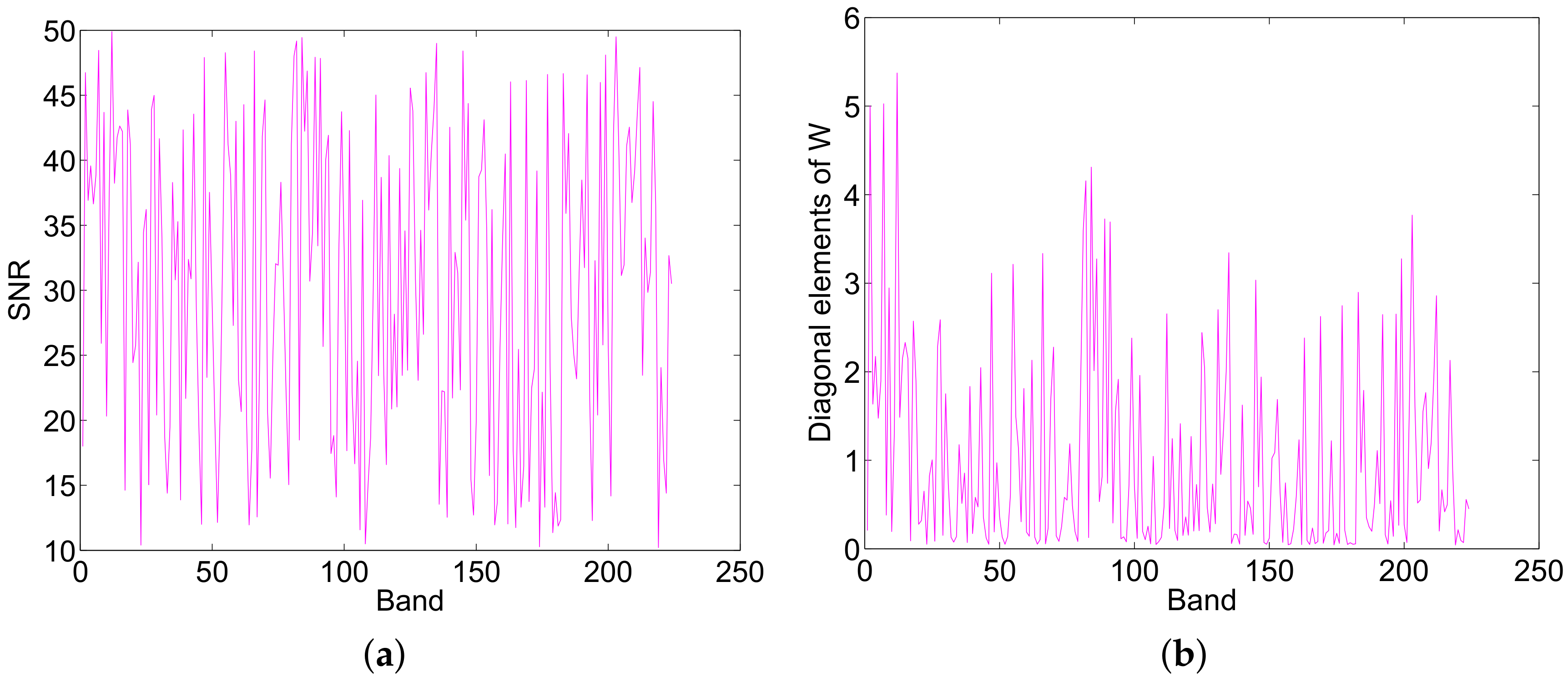
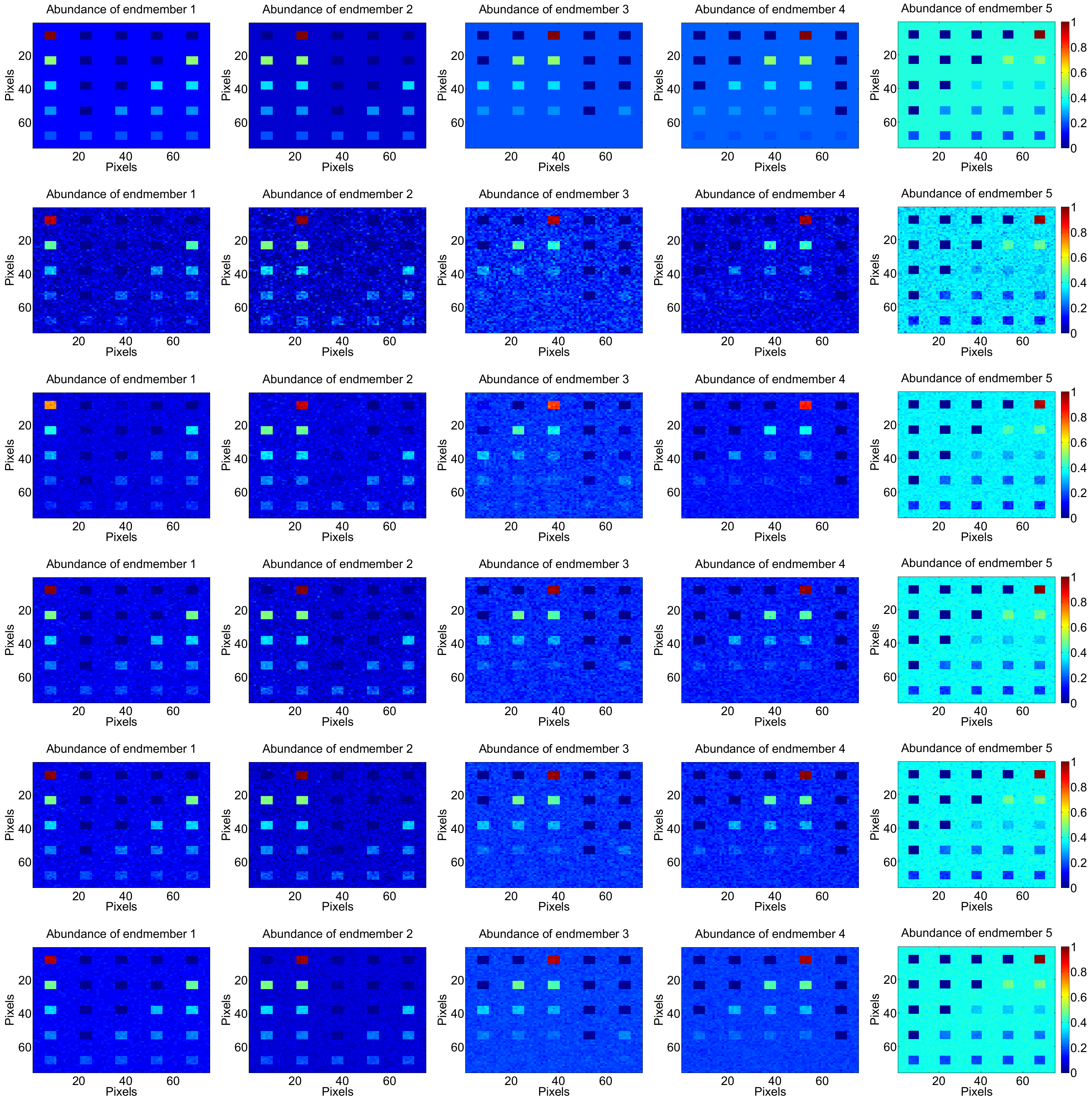
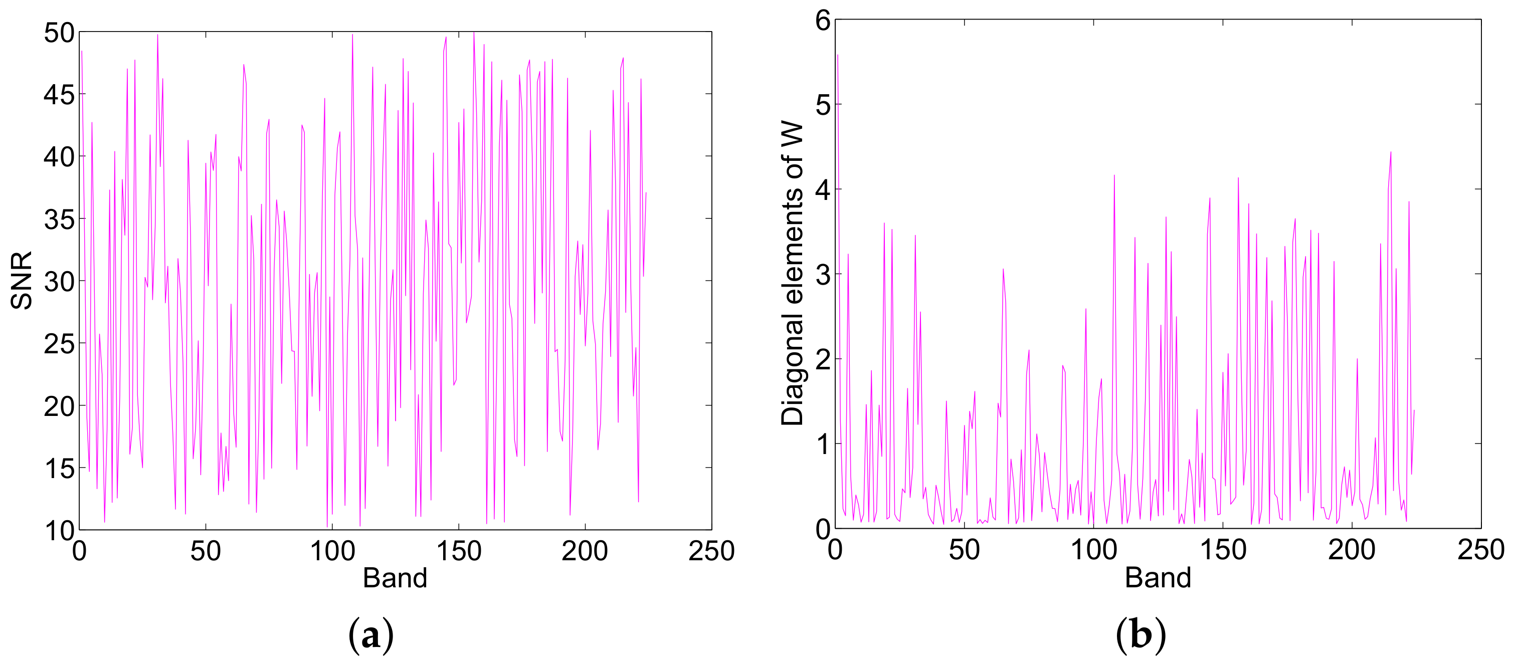
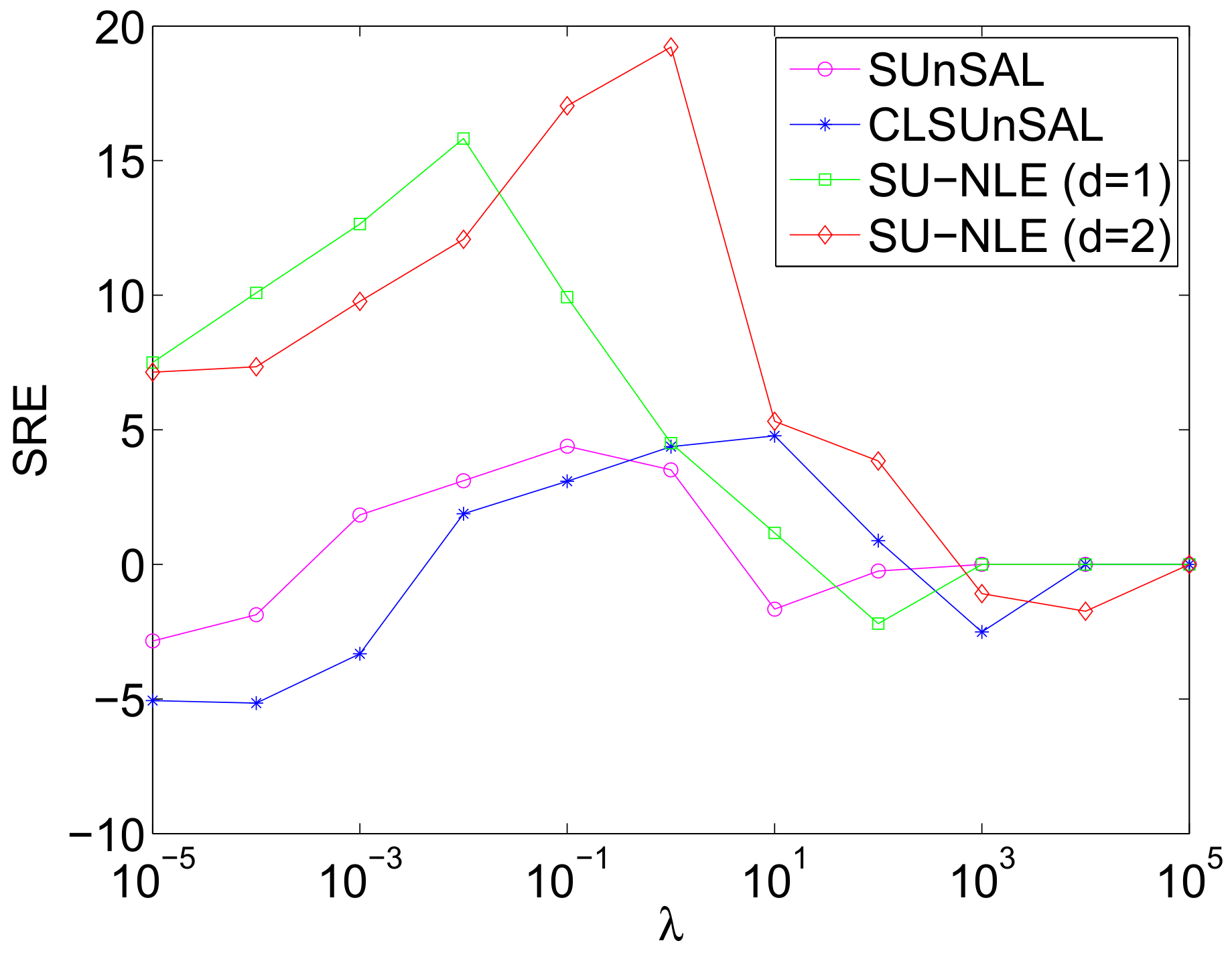
In this experiment, the simulated HSI, of 75 × 75 pixels and 224 bands, is generated based on the LMM. Five endmembers are randomly selected from the spectral library that have 240 endmembers, and the abundances of the 5 selected endmembers are generated in the same way as in [37]. The code to generate the abundance maps is available at http://www.lx.it.pt/~bioucas/publications.html. There are both pure and mixed regions in the resulted HSI, and the mixtures are made up of two to 5 endmembers, which are distributed spatially in the form of distinct square regions. The generated abundances of the 5 selected spectral signatures are shown in Figure 4, which indicates that both pure and mixed regions exist in the simulated HSI. The background pixels comprise mixtures of the 5 endmembers, where their abundances are randomly fixed to 0.1149, 0.0741, 0.2003, 0.2055, and 0.4051. The data cubes obtained are then degraded by Gaussian white noise, and the SNRs of the different HSI bands are different ranging from 20 dB to 40 dB, which is shown in Figure 5a, and the mean SNR is 30.12 dB. Figure 5b shows the diagonal elements of weighting matrix of the proposed SU-NLE, and it can be observed from Figure 5a,b that the fluctuation of the SNR of different bands is quite in accordance with the diagonal elements of weighting matrix, which demonstrates the efficiency of the estimation of the level of noise in each band. Besides, Figure 6 shows the SREs of the methods SU-NLE, SUnSAL and CLSUnSAL as a function of varying regularization parameter . As shown in Figure 6, the SREs of SUnSAL, CLSUnSAL, SU-NLE () and SU-NLE () first increase as increases, and obtain the best SREs when , respectively. The SREs of SUnSAL, CLSUnSAL, SU-NLE () and SU-NLE () then decrease when increases to a certain level. Besides, the SREs of some methods approximate to 0 when . This is due to sparsity dominating the solution, which makes all the estimated abundances be nearly 0 when is too big. In addition, the SREs of SU-NLE () and SU-NLE () are higher than those of SUnSAL and CLSUnSAL when , respectively, because SU-NLE () and SU-NLE () adopt the weighting strategy that considers the different noise levels of different bands, which demonstrates the efficiency of integrating noise level estimation into the sparse regression unmixing framework. Moreover, Figure 4 shows the abundance maps of 5 endmembers for different methods when tuning the performance of all methods to their best SREs. As shown in Figure 4, the abundance maps of the 5 endmembers for SU-NLE () and SU-NLE () approximate better to the ground-truth abundance maps than those of SUnSAL and CLSUnSAL, which also demonstrates the efficiency of integrating noise level estimation into the sparse regression unmixing framework.
3.1.2. Simulated experiment II
In this simulated experiment, we generate simulated HSIs without pure regions. We adopt the approach in [61] to generate the abundances, and the code is available at: https://bitbucket.org/aicip/mvcnmf. The synthetic HSI has pixels without pure pixels using the above mentioned spectral library that have 240 endmembers. The HSI is divided into regions, and each region has pixels, where q controls the region size and HSI image size. All pixels in each region have the same type of ground cover, randomly selected as one of the endmember classes, then the spatial low-pass filter of size has been applied to the HSI to create mixed pixels. All pixels with abundances greater than 80% are replaced by a mixture of all endmembers with equally distributed abundances, which aims to further remove pure pixels, and the generated true abundances are shown in Figure 7. The data cubes obtained are then degraded by Gaussian white noise, and the SNRs of the different HSI bands vary and range from 10 dB to 50 dB, which is shown in Figure 8a, and the mean SNR is 30.33 dB. Figure 8b shows the diagonal elements of weighting matrix of the proposed SU-NLE, and it can be seen from Figure 8a,b that the fluctuation of the SNR of different bands is quite in accordance with the diagonal elements of weighting matrix, which demonstrates the efficiency of the estimation of the level of noise in each band. Figure 9 shows the SREs of the methods SU-NLE, SUnSAL and CLSUnSAL as a function of the varying regularization parameter when q = 8 and the number of endmembers is 4. As shown in Figure 9, the SREs of SUnSAL, SU-NLE (), and SU-NLE () first increase as increases, and they obtain the best SREs at different . The SREs of SUnSAL, CLSUnSAL, SU-NLE (), and SU-NLE () then decrease when increases to a certain level. The SREs of some methods approximate to 0 when . This is due to sparsity dominating the solution, which makes all the estimated abundances be nearly 0 when is too big, so it is meaningless to set too large. Besides, the SREs of SU-NLE () and SU-NLE () are evidently higher than those of SUnSAL and CLSUnSAL when , respectively, which demonstrates that considering the different noise levels in different bands efficiently improves the performance of sparse unmixing. Moreover, Figure 7 shows the abundance maps obtained by the proposed and compared methods contaminated by Gaussian white noise when q = 8 and the number of endmembers is 4. Figure 7 also shows that the abundance maps obtained by the SU-NLE () and SU-NLE () are more similar to the true abundance maps than those of SUnSAL and CLSUnSAL, because the SU-NLE () and SU-NLE () adopt the weighting strategy to consider the noise levels in different bands.
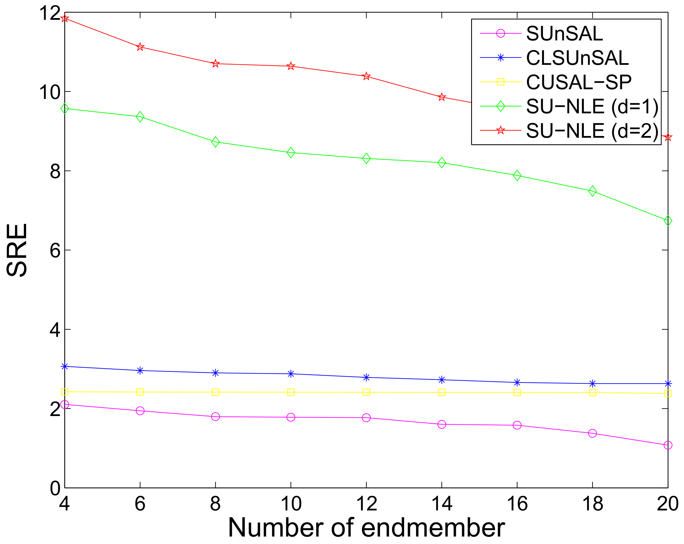
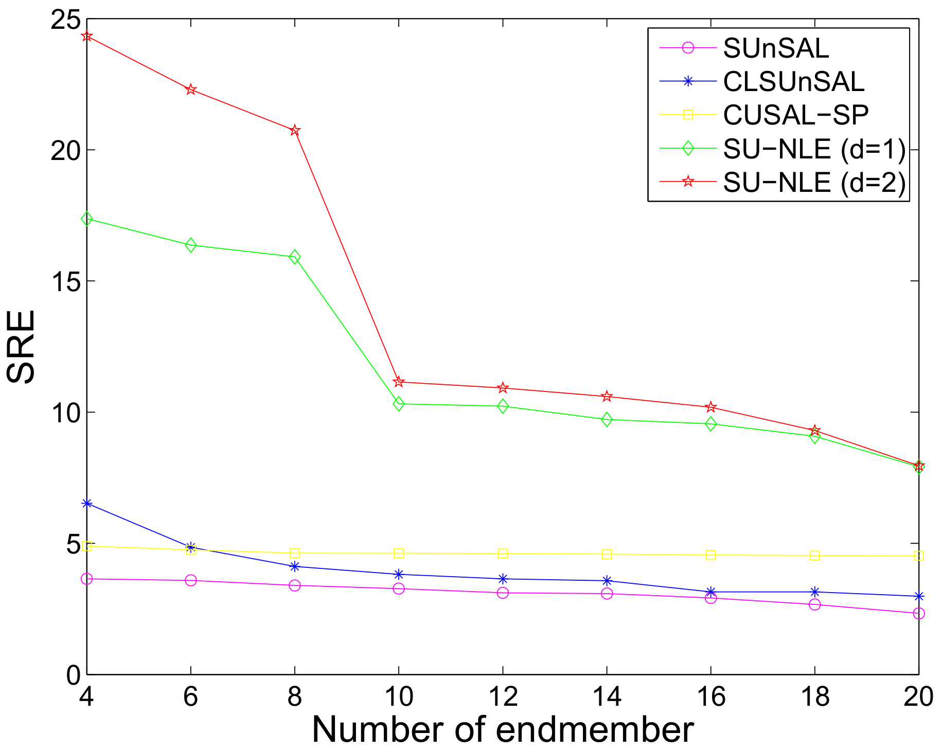
We also study the influence of the number of endmembers on the final unmixing performance. To avoid unnecessary deviation, we perform the simulations 100 times to obtain the mean SREs. The setting for this experiment is as follows: image size is , q = 8, filter size is , the SNR ranges from 10 dB to 50 dB, and all methods have tuned to their best SREs. Figure 10 shows the SREs of the proposed and compared methods as a function of the varying number of endmembers under Gaussian white noise with only mixed regions having 64 × 64 pixels and 224 bands. Figure 10 also shows that the SREs generally decrease as the number of endmembers increases, because the spectral signatures in the selected spectral library are usually highly correlated. In addition, the SREs of SU-NLE () and SU-NLE () are higher than those of SUnSAL and CLSUnSAL for all numbers of endmembers, respectively, which also demonstrates that the performance of sparse unmixing can be improved by considering the different noise levels in different bands.
Moreover, we study the influence of image size on the final unmixing performance when the number of endmembers is 4. We also perform the simulations 100 times to obtain the mean SREs. The setting for this experiment is as follows: q ranges from 6 to 10, which makes the image size range from to ; the SNRs of different bands for all of the different image sizes range from 10 dB to 50 dB. Figure 11 shows the SREs of the proposed and compared methods as a function of varying image size under Gaussian white noise with only mixed regions having 64 × 64 pixels, 4 endmembers and 224 bands. As shown in Figure 11, the SREs of SU-NLE () and SU-NLE () are higher than those of SUnSAL and CLSUnSAL for different image sizes, respectively, which also demonstrates the importance of adopting the weighting strategy in the sparse regression unmixing framework. In addition, the SREs of the proposed and compared methods remain stable with the different HSI sizes, which demonstrates that the performance of regression-based unmixing methods is not sensitive to image size.
3.1.3. Simulated experiment III
In this simulation, we conduct experiments of contamination by correlated noise. Considering that calibrating the HSI obtained from an airborne or spaceborne sensor is difficult, the noise and the spectra in real HSIs are usually of low-pass type, which makes the noise highly correlated [27]. Thus, experiments need to be conducted when the obtained HSI is contaminated by correlated noise. We generate simulated HSIs using 5 randomly selected spectral signatures from the library on the basis of LMM, which has pure and mixed regions that have 75 × 75 pixels and 224 bands. We adopt the same approach in Simulated Experiment I to generate the abundance, which are shown in Figure 12. The mixtures range from two to 5 endmembers, and the background pixels comprise mixtures of the 5 endmembers, where their abundances are randomly fixed to 0.1149, 0.0741, 0.2003, 0.2055, and 0.4051. The HSI obtained is then contaminated with correlated noise, and the correlated noise is generated using the same approach as in [33]. The correlated noise function is available at http://www.mathworks.com/matlabcentral/fileexchange/21156-correlated-Gaussian-noise/content/correlatedGaussianNoise.m, and the correlation matrix is set as default. The SNR of each band of HSI ranges from 20 dB to 40 dB, which is shown in Figure 13a, and the mean SNR is 30.12 dB. Figure 13b shows the diagonal elements of weighting matrix of the proposed SU-NLE, and it can be seen from Figure 13a,b that the fluctuation of the SNR of different bands is quite in accordance with the diagonal elements of weighting matrix, which demonstrates the efficiency of the estimation of the level of noise in each band. Figure 14 shows the SREs of the SU-NLE, SUnSAL and CLSUnSAL as a function of varying regularization parameter under correlated noise with both pure and mixed regions having 75 × 75 pixels and 224 bands. As shown in Figure 14, the SREs of SUnSAL, SU-NLE (), and SU-NLE () first increase as increases, and they obtain the best SREs at different . Then, they decrease when increases to a certain level. The SREs of some methods approximate to 0 when , and the underlying reason is that sparsity dominates the solution. The estimated abundances be nearly 0 when is too big, so it is meaningless to set too large. Besides, the SREs of SU-NLE () and SU-NLE () are considerably higher than those of SUnSAL and CLSUnSAL when , respectively, which demonstrates the efficiency of integrating noise level estimation into the sparse regression unmixing framework. Moreover, Figure 12 shows the abundance maps of 5 endmembers for different methods under correlated noise with both pure and mixed regions having 75 × 75 pixels and 224 bands when tuning the performance of all methods to the optimal SREs. As shown in Figure 12, the abundance maps of the 5 endmembers for the SU-NLE () and SU-NLE () are more similar to the ground-truth abundance maps than those of SUnSAL and CLSUnSAL, which also demonstrates that the unmixing performance can be improved by integrating noise level estimation into the sparse regression unmixing framework.
3.1.4. Simulated experiment IV
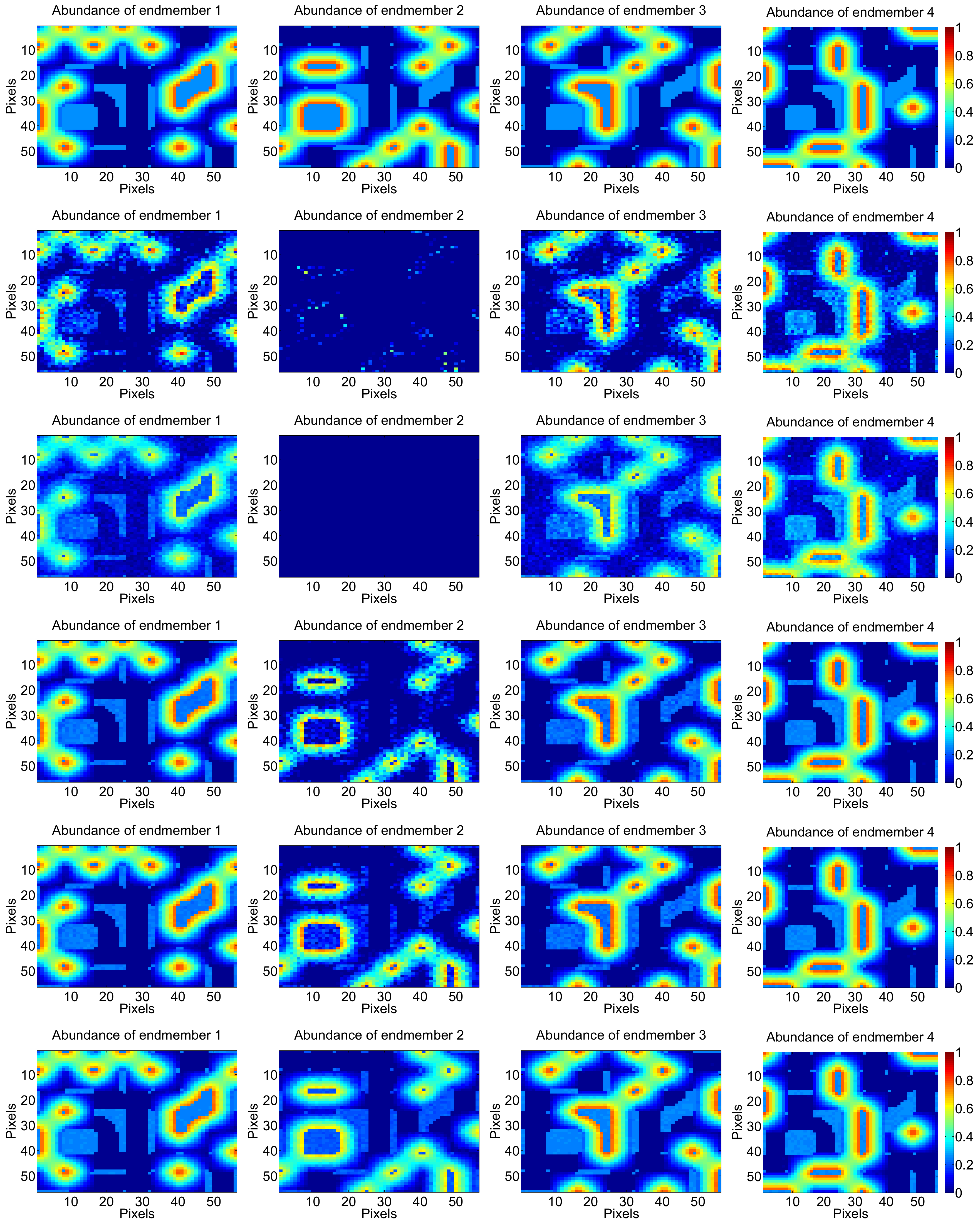
In this simulated experiment, we generate simulated HSIs without pure regions under correlated noise. We adopt the same approach in Simulated Experiment II to generate the abundance, and the generated true abundances are shown in Figure 15. The data cubes obtained are then degraded by correlated noise, the SNRs of the different HSI bands are shown in Figure 16a ranging from 10 dB to 50 dB, and the mean SNR is 30.12 dB. Figure 16b shows the diagonal elements of weighting matrix of the proposed SU-NLE, and it can be seen from Figure 16a,b that the fluctuation of the SNR of different bands is quite in accordance with the diagonal elements of weighting matrix, which demonstrates the efficiency of the estimation of the level of noise in each band. Figure 17 shows the SREs of the methods SU-NLE, SUnSAL and CLSUnSAL as a function of varying regularization parameter under correlated noise with only mixed regions having 64 × 64 pixels and 224 bands. As shown in Figure 17, the SREs of SUnSAL, SU-NLE (), and SU-NLE () first increase as increases, and they obtain the best SREs at different . The SREs of SUnSAL, CLSUnSAL, SU-NLE (), and SU-NLE () then decrease when increases to a certain level. The SREs of some methods approximate to 0 when . This is due to sparsity dominating the solution, which makes all the estimated abundances be nearly 0 when is too big, so it is meaningless to set too large. Besides, the SREs of SU-NLE () and SU-NLE () are higher than those of SUnSAL and CLSUnSAL when , respectively, which demonstrates the efficiency of considering the different noise levels in different bands to improve the unmixing performance. Moreover, Figure 15 shows the abundance maps of 4 endmembers for different methods under correlated noise with only mixed regions having 64 × 64 pixels and 224 bands, and the estimated abundances of endmember 2 using SUnSAL and CLSUnSAL fail badly. While the estimated abundances of endmember 2 using the SU-NLE () and SU-NLE () approximate obviously better to the ground truth. Figure 15 also shows that the abundance maps obtained by the SU-NLE () and SU-NLE () approximate better to the true abundance maps than those of SUnSAL and CLSUnSAL, because the SU-NLE () and SU-NLE () use the weighting strategy to consider the different noise levels in different bands.
We also study the influence of the number of endmembers on the final unmixing performance when contaminated by correlated noise. We also perform the simulations 100 times to obtain the mean SREs. The setting for this experiment is as follows: image size is , q = 8, filter size is , and the SNRs of different bands range from 10 dB to 50 dB. Figure 18 shows the SREs of different methods as a function of varying number of endmember under correlated noise with only mixed regions having 64 × 64 pixels and 224 bands. Figure 18 also shows that the SREs generally decrease as the number of endmembers increases, because the spectral signatures are usually highly correlated. For all numbers of endmembers, the SREs of SU-NLE () and SU-NLE () are substantially higher than those of SUnSAL and CLSUnSAL, respectively, which also demonstrates that the integration of the weighting strategy into the sparse regression framework helps improve the unmixing performance.
Moreover, we study the influence of image size on the final unmixing performance under correlated noise when the number of endmembers is 4. We also perform the simulations 100 times to obtain the mean SREs. The setting for this experiment is as follows: q ranges from 6 to 10, which makes the image size range from to ; the SNRs of different bands for all of the different image sizes range from 10 dB to 50 dB. Figure 19 shows the SREs of different methods as a function of varying image size under correlated white noise with only mixed regions having 64 × 64 pixels, 4 endmembers and 224 bands. As shown in Figure 19, the SREs of SU-NLE () and SU-NLE () are markedly higher than those of SUnSAL and CLSUnSAL for different image sizes, respectively, which demonstrates the importance of adopting the weighting strategy into sparse regression unmixing framework. The SREs of SUnSAL, CLSUnSAL, and SU-NLE () remain stable for different image sizes, and the SRE of SU-NLE () increases slowly as the image size increases.
In summary, the integration of noise level estimation to the sparse unmixing of HSI is important. In addition, the proposed method can achieve excellent unmixing performance for different noise levels in different bands, noise types, numbers of endmembers, and image sizes, which demonstrates the efficiency of the proposed method.
3.2. Experimental Results with Real Data
In the experiment on real data, we adopt the most benchmarked dataset for hyperspectral unmixing, which was captured by Airborne Visible/Infrared Imaging Spectrometer (AVIRIS) over a Cuprite mining district in June 1997 in Nevada. Several spectral bands (1–2, 104–113, 148–167 and 221–224) have been removed due to noise corruption and atmospheric absorption, leaving D = 188 spectral bands that range from 0.4 m to 2.5 m with a nominal bandwidth of 10 nm. The false color image is shown in Figure 20, which is of size .
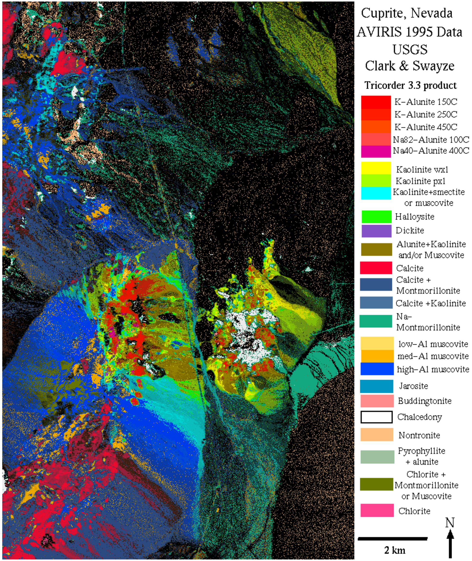
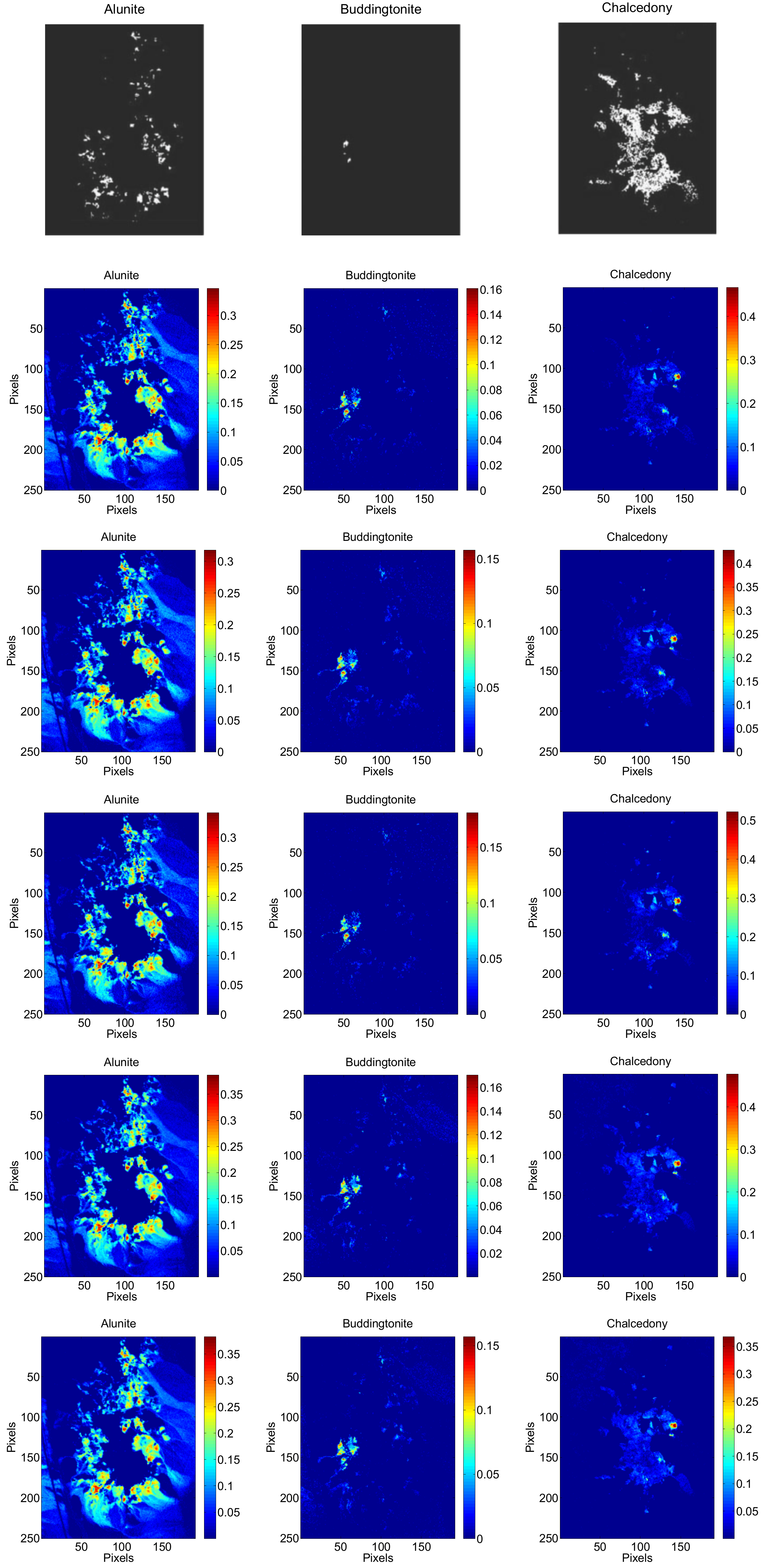
The Cuprite is mineralogical, and the exposed minerals are all included in the USGS library considered in the simulated experiments. Thus, we adopt the same USGS library in the simulated experiments for the sparse unmixing of Cuprite, which has 240 endmembers. Figure 21 shows the mineral map of the selected Cuprite image, which is available at http://speclab.cr.usgs.gov/cuprite95.tgif.2.2um_map.gif. The Tricorder 3.3 software product [62] was used to map different minerals present in the Cuprite mining district, and the USGS map can be served as a good indicator for qualitative assessment of the fractional abundance maps produced by the different unmixing methods [27,37,40]. Besides, Figure 22 shows the diagonal elements of the weighting matrix of the proposed SU-NLE, which can estimate the noise level in different band of Cuprite. Moreover, Figure 23 shows the fractional abundance maps of three representative endmembers estimated by different unmixing methods using Cuprite dataset having pixels and 188 bands. The regularization parameters are chosen for different methods that approximate best to the USGS Tetracorder classification map as follows: SUnSAL (), CLSUnSAL (), CUSAL-SP (), SU-NLE () () and SU-NLE () (). As shown in Figure 23, the estimated abundances maps of Chalcedony using SU-NLE () and SU-NLE () approximate to the USGS Tetracorder classification map of Chalcedony obviously better than the SUnSAL and CLSUnSAL, respectively, which demonstrates the efficiency of integrating noise level estimation into the sparse regression unmixing framework. Furthermore, the average numbers of endmembers with abundances higher than 0.05 estimated by SUnSAL, CLSUnSAL, CUSAL-SP, SU-NLE () and SU-NLE () are 5.124, 5.014, 4.620, 4.486 and 4.382, respectively (per pixel). These differences lead to the conclusion that SU-NLE uses a smaller number of endmembers to explain the data, thus enforcing sparsity. The average number of endmembers with abundances higher than 0.05 estimated by SU-NLE () and SUnSAL are higher than these of SU-NLE () and CLSUnSAL, respectively, which leads to the conclusion that SU-NLE () and CLSUnSAL enforce the sparseness both at the group and individual levels.
4. Conclusions
In this paper, we propose a general sparse unmixing method based on noise level estimation. The weighting strategy is adopted to obtain the noise weighting matrix, which can be integrated into the sparse regression unmixing framework to improve the performance of sparse unmixing. The proposed SU-NLE is robust for different noise levels in different bands in the sparse unmixing of HSI, and it can be solved by ADMM. Moreover, the proposed method can obtain better unmixing performance than other popular sparse unmixing methods on both synthetic datasets and real HSIs, which demonstrates the efficiency of the strategy of integrating noise level estimation into the sparse unmixing of HSI.
Acknowledgments
Financial support for this study was provided by the National Natural Science Foundation of China under Grants 61773295, 61503288 and 61605146, and the China Postdoctoral Science Foundation under Grants 2017M612504, 2016M592385 and 2016T90725.
Author Contributions
All authors have made great contributions to the work. Chang Li, Yong Ma and Jiayi Ma designed the research and analyzed the results. Chang Li, Xiaoguang Mei, Fan Fan, and Jun Huang performed the experiments and wrote the manuscript. Jiayi Ma gave insightful suggestions to the work and revised the manuscript.
Conflicts of Interest
The authors declare no conflict of interest.
References
- Williams, M.D.; Parody, R.J.; Fafard, A.J.; Kerekes, J.P.; van Aardt, J. Validation of Abundance Map Reference Data for Spectral Unmixing. Remote Sens. 2017, 9, 473. [Google Scholar] [CrossRef]
- Fan, H.; Chen, Y.; Guo, Y.; Zhang, H.; Kuang, G. Hyperspectral Image Restoration Using Low-Rank Tensor Recovery. IEEE J. Sel. Top. Appl. Earth Obs. Remote Sens. 2017, 10, 4589–4604. [Google Scholar] [CrossRef]
- Ahmed, A.M.; Duran, O.; Zweiri, Y.; Smith, M. Hybrid Spectral Unmixing: Using Artificial Neural Networks for Linear/Non-Linear Switching. Remote Sens. 2017, 9, 775. [Google Scholar] [CrossRef]
- Sui, C.; Tian, Y.; Xu, Y.; Xie, Y. Unsupervised band selection by integrating the overall accuracy and redundancy. IEEE Geosci. Remote Sens. Lett. 2015, 12, 185–189. [Google Scholar]
- Li, Y.; Tao, C.; Tan, Y.; Shang, K.; Tian, J. Unsupervised multilayer feature learning for satellite image scene classification. IEEE Geosci. Remote Sens. Lett. 2016, 13, 157–161. [Google Scholar] [CrossRef]
- Li, Y.; Huang, X.; Liu, H. Unsupervised deep feature learning for urban village detection from high-resolution remote sensing images. Photogramm. Eng. Remote Sens. 2017, 83, 567–579. [Google Scholar] [CrossRef]
- Ghasrodashti, E.K.; Karami, A.; Heylen, R.; Scheunders, P. Spatial Resolution Enhancement of Hyperspectral Images Using Spectral Unmixing and Bayesian Sparse Representation. Remote Sens. 2017, 9, 541. [Google Scholar]
- Li, C.; Ma, Y.; Mei, X.; Liu, C.; Ma, J. Hyperspectral Image Classification With Robust Sparse Representation. IEEE Geosci. Remote Sens. Lett. 2016, 13, 641–645. [Google Scholar] [CrossRef]
- Li, Y.; Zhang, Y.; Huang, X.; Zhu, H.; Ma, J. Large-Scale Remote Sensing Image Retrieval by Deep Hashing Neural Networks. IEEE Trans. Geosci. Remote Sens. 2017, in press. [Google Scholar] [CrossRef]
- Sui, C.; Tian, Y.; Xu, Y.; Xie, Y. Weighted Spectral-Spatial Classification of Hyperspectral Images via Class-Specific Band Contribution. IEEE Trans. Geosci. Remote Sens. 2017, 1–15. [Google Scholar] [CrossRef]
- Ma, J.; Zhou, H.; Zhao, J.; Gao, Y.; Jiang, J.; Tian, J. Robust Feature Matching for Remote Sens. Image Registration via Locally Linear Transforming. IEEE Trans. Geosci. Remote Sens. 2015, 53, 6469–6481. [Google Scholar] [CrossRef]
- Yang, K.; Pan, A.; Yang, Y.; Zhang, S.; Ong, S.H.; Tang, H. Remote Sensing Image Registration Using Multiple Image Features. Remote Sens. 2017, 9, 581. [Google Scholar] [CrossRef]
- Wei, Z.; Han, Y.; Li, M.; Yang, K.; Yang, Y.; Luo, Y.; Ong, S.H. A Small UAV Based Multi-Temporal Image Registration for Dynamic Agricultural Terrace Monitoring. Remote Sens. 2017, 9, 904. [Google Scholar] [CrossRef]
- Esmaeili Salehani, Y.; Gazor, S.; Kim, I.M.; Yousefi, S. l0-Norm Sparse Hyperspectral Unmixing Using Arctan Smoothing. Remote Sens. 2016, 8, 187. [Google Scholar] [CrossRef]
- Bioucas-Dias, J.M.; Plaza, A.; Dobigeon, N.; Parente, M.; Du, Q.; Gader, P.; Chanussot, J. Hyperspectral unmixing overview: Geometrical, statistical, and sparse regression-based approaches. IEEE J. Sel. Top. Appl. Earth Obs. Remote Sens. 2012, 5, 354–379. [Google Scholar] [CrossRef]
- Liu, R.; Du, B.; Zhang, L. Hyperspectral unmixing via double abundance characteristics constraints based NMF. Remote Sens. 2016, 8, 464. [Google Scholar] [CrossRef]
- Li, C.; Ma, Y.; Huang, J.; Mei, X.; Liu, C.; Ma, J. GBM-Based Unmixing of Hyperspectral Data Using Bound Projected Optimal Gradient Method. IEEE Geosci. Remote Sens. Lett. 2016, 13, 952–956. [Google Scholar] [CrossRef]
- Themelis, K.; Rontogiannis, A.A.; Koutroumbas, K. Semi-Supervised Hyperspectral Unmixing via the Weighted Lasso. In Proceedings of the 35th International Conference on Acoustics, Speech, and Signal Processing (ICASSP), Dallas, TX, USA, 15–19 March 2010; pp. 1194–1197. [Google Scholar]
- Heinz, D.C.; Chang, C.I. Fully constrained least squares linear spectral mixture analysis method for material quantification in hyperspectral imagery. IEEE Trans. Geosci. Remote Sens. 2001, 39, 529–545. [Google Scholar] [CrossRef]
- Winter, M.E. N-FINDR: An algorithm for fast autonomous spectral end-member determination in hyperspectral data. In Proceedings of the SPIE’s International Symposium on Optical Science, Engineering, and Instrumentation, Denver, CO, USA, 27 October 1999; International Society for Optics and Photonics: Bellingham, DC, USA, 1999; pp. 266–275. [Google Scholar]
- Nascimento, J.M.; Dias, J.M. Vertex component analysis: A fast algorithm to unmix hyperspectral data. IEEE Trans. Geosci. Remote Sens. 2005, 43, 898–910. [Google Scholar] [CrossRef]
- Nascimento, J.M.; Dias, J.M. Does independent component analysis play a role in unmixing hyperspectral data? IEEE Trans. Geosci. Remote Sens. 2005, 43, 175–187. [Google Scholar] [CrossRef]
- Wang, J.; Chang, C.I. Applications of independent component analysis in endmember extraction and abundance quantification for hyperspectral imagery. IEEE Trans. Geosci. Remote Sens. 2006, 44, 2601–2616. [Google Scholar] [CrossRef]
- Pauca, V.P.; Piper, J.; Plemmons, R.J. Nonnegative matrix factorization for spectral data analysis. Linear Algebra Appl. 2006, 416, 29–47. [Google Scholar] [CrossRef]
- Jia, S.; Qian, Y. Constrained nonnegative matrix factorization for hyperspectral unmixing. IEEE Trans. Geosci. Remote Sens. 2009, 47, 161–173. [Google Scholar] [CrossRef]
- Qian, Y.; Jia, S.; Zhou, J.; Robles-Kelly, A. Hyperspectral unmixing via sparsity-constrained nonnegative matrix factorization. IEEE Trans. Geosci. Remote Sens. 2011, 49, 4282–4297. [Google Scholar] [CrossRef]
- Iordache, M.D.; Bioucas-Dias, J.M.; Plaza, A. Sparse unmixing of hyperspectral data. IEEE Trans. Geosci. Remote Sens. 2011, 49, 2014–2039. [Google Scholar] [CrossRef]
- Ma, J.; Zhao, J.; Tian, J.; Bai, X.; Tu, Z. Regularized vector field learning with sparse approximation for mismatch removal. Pattern Recognit. 2013, 46, 3519–3532. [Google Scholar] [CrossRef]
- Gao, Y.; Ma, J.; Yuille, A.L. Semi-Supervised Sparse Representation Based Classification for Face Recognition With Insufficient Labeled Samples. IEEE Trans. Image Process. 2017, 26, 2545–2560. [Google Scholar] [CrossRef] [PubMed]
- Ma, J.; Jiang, J.; Liu, C.; Li, Y. Feature guided Gaussian mixture model with semi-supervised EM and local geometric constraint for retinal image registration. Inf. Sci. 2017, 417, 128–142. [Google Scholar] [CrossRef]
- Akhtar, N.; Shafait, F.; Mian, A. Futuristic greedy approach to sparse unmixing of hyperspectral data. IEEE Trans. Geosci. Remote Sens. 2015, 53, 2157–2174. [Google Scholar] [CrossRef]
- Tang, W.; Shi, Z.; Wu, Y. Regularized simultaneous forward-backward greedy algorithm for sparse unmixing of hyperspectral data. IEEE Trans. Geosci. Remote Sens. 2014, 52, 5271–5288. [Google Scholar] [CrossRef]
- Shi, Z.; Tang, W.; Duren, Z.; Jiang, Z. Subspace matching pursuit for sparse unmixing of hyperspectral data. IEEE Trans. Geosci. Remote Sens. 2014, 52, 3256–3274. [Google Scholar] [CrossRef]
- Fu, X.; Ma, W.K.; Chan, T.H.; Bioucas-Dias, J. Self-Dictionary Sparse Regression for Hyperspectral Unmixing: Greedy Pursuit and Pure Pixel Search Are Related. IEEE J. Sel. Top. Appl. Earth Obs. Remote Sens. 2015, 9, 1128–1141. [Google Scholar] [CrossRef]
- Zhang, G.; Xu, Y.; Fang, F. Framelet-Based Sparse Unmixing of Hyperspectral Images. IEEE Trans. Image Process. 2016, 25, 1516–1529. [Google Scholar] [CrossRef] [PubMed]
- Bioucas-Dias, J.M.; Figueiredo, M.A. Alternating direction algorithms for constrained sparse regression: Application to hyperspectral unmixing. In Proceedings of the 2010 2nd Workshop on Hyperspectral Image and Signal Processing: Evolution in Remote Sensing, Reykjavìk, Iceland, 14–16 June 2010; pp. 1–4. [Google Scholar]
- Iordache, M.D.; Bioucas-Dias, J.M.; Plaza, A. Total variation spatial regularization for sparse hyperspectral unmixing. IEEE Trans. Geosci. Remote Sens. 2012, 50, 4484–4502. [Google Scholar] [CrossRef]
- Mei, S.; Du, Q.; He, M. Equivalent-Sparse Unmixing Through Spatial and Spectral Constrained Endmember Selection From an Image-Derived Spectral Library. IEEE J. Sel. Top. Appl. Earth Obs. Remote Sens. 2015, 8, 2665–2675. [Google Scholar] [CrossRef]
- Zhong, Y.; Feng, R.; Zhang, L. Non-local sparse unmixing for hyperspectral remote sensing imagery. IEEE J. Sel. Top. Appl. Earth Obs. Remote Sens. 2014, 7, 1889–1909. [Google Scholar] [CrossRef]
- Iordache, M.D.; Bioucas-Dias, J.M.; Plaza, A. Collaborative sparse regression for hyperspectral unmixing. IEEE Trans. Geosci. Remote Sens. 2014, 52, 341–354. [Google Scholar] [CrossRef]
- Zheng, C.Y.; Li, H.; Wang, Q.; Chen, C.P. Reweighted Sparse Regression for Hyperspectral Unmixing. IEEE Trans. Geosci. Remote Sens. 2016, 54, 479–488. [Google Scholar] [CrossRef]
- Feng, R.; Zhong, Y.; Zhang, L. Adaptive Spatial Regularization Sparse Unmixing Strategy Based on Joint MAP for Hyperspectral Remote Sens. Imagery. IEEE J. Sel. Top. Appl. Earth Obs. Remote Sens. 2016, 9, 5791–5805. [Google Scholar] [CrossRef]
- Li, C.; Ma, Y.; Mei, X.; Liu, C.; Ma, J. Hyperspectral unmixing with robust collaborative sparse regression. Remote Sens. 2016, 8, 588. [Google Scholar] [CrossRef]
- Ma, Y.; Li, C.; Mei, X.; Liu, C.; Ma, J. Robust Sparse Hyperspectral Unmixing With ℓ2,1 Norm. IEEE Trans. Geosci. Remote Sens. 2017, 55, 1227–1239. [Google Scholar] [CrossRef]
- Chen, F.; Zhang, Y. Sparse Hyperspectral Unmixing Based on Constrained lp-l 2 Optimization. IEEE Geosci. Remote Sens. Lett. 2013, 10, 1142–1146. [Google Scholar] [CrossRef]
- Xu, Y.; Fang, F.; Zhang, G. Similarity-Guided and-Regularized Sparse Unmixing of Hyperspectral Data. IEEE Geosci. Remote Sens. Lett. 2015, 12, 2311–2315. [Google Scholar] [CrossRef]
- Themelis, K.E.; Rontogiannis, A.A.; Koutroumbas, K.D. A novel hierarchical Bayesian approach for sparse semisupervised hyperspectral unmixing. IEEE Trans. Signal Process. 2012, 60, 585–599. [Google Scholar] [CrossRef]
- Xu, X.; Shi, Z. Multi-objective based spectral unmixing for hyperspectral images. ISPRS J. Photogramm. Remote Sens. 2017, 124, 54–69. [Google Scholar] [CrossRef]
- Tang, W.; Shi, Z.; Wu, Y.; Zhang, C. Sparse Unmixing of Hyperspectral Data Using Spectral A Priori Information. IEEE Trans. Geosci. Remote Sens. 2015, 53, 770–783. [Google Scholar] [CrossRef]
- Wang, Y.; Pan, C.; Xiang, S.; Zhu, F. Robust hyperspectral unmixing with correntropy-based metric. IEEE Trans. Image Process. 2015, 24, 4027–4040. [Google Scholar] [CrossRef] [PubMed]
- Zhu, F.; Halimi, A.; Honeine, P.; Chen, B.; Zheng, N. Correntropy Maximization via ADMM: Application to Robust Hyperspectral Unmixing. IEEE Trans. Geosci. Remote Sens. 2017, 55, 4944–4955. [Google Scholar] [CrossRef]
- Bioucas-Dias, J.M.; Nascimento, J.M. Hyperspectral subspace identification. IEEE Trans. Geosci. Remote Sens. 2008, 46, 2435–2445. [Google Scholar] [CrossRef]
- Uss, M.L.; Vozel, B.; Lukin, V.V.; Chehdi, K. Local signal-dependent noise variance estimation from hyperspectral textural images. IEEE J. Sel. Top. Signal Process. 2011, 5, 469–486. [Google Scholar] [CrossRef]
- Gao, L.; Du, Q.; Zhang, B.; Yang, W.; Wu, Y. A comparative study on linear regression-based noise estimation for hyperspectral imagery. IEEE J. Sel. Top. Appl. Earth Obs. Remote Sens. 2013, 6, 488–498. [Google Scholar] [CrossRef]
- Eldar, Y.C.; Rauhut, H. Average case analysis of multichannel sparse recovery using convex relaxation. IEEE Trans. Inf. Theory 2010, 56, 505–519. [Google Scholar] [CrossRef]
- Ma, J.; Chen, C.; Li, C.; Huang, J. Infrared and visible image fusion via gradient transfer and total variation minimization. Inf. Fusion 2016, 31, 100–109. [Google Scholar] [CrossRef]
- Boyd, S.; Parikh, N.; Chu, E.; Peleato, B.; Eckstein, J. Distributed optimization and statistical learning via the alternating direction method of multipliers. Found. Trends Mach. Learn. 2011, 3, 1–122. [Google Scholar] [CrossRef]
- Donoho, D.L. De-noising by soft-thresholding. IEEE Trans. Inf. Theory 1995, 41, 613–627. [Google Scholar] [CrossRef]
- Wright, S.J.; Nowak, R.D.; Figueiredo, M.A. Sparse reconstruction by separable approximation. IEEE Trans. Signal Process. 2009, 57, 2479–2493. [Google Scholar] [CrossRef]
- Hoyer, P.O. Non-negative matrix factorization with sparseness constraints. J. Mach. Learn. Res. 2004, 5, 1457–1469. [Google Scholar]
- Miao, L.; Qi, H. Endmember extraction from highly mixed data using minimum volume constrained nonnegative matrix factorization. IEEE Trans. Geosci. Remote Sens. 2007, 45, 765–777. [Google Scholar] [CrossRef]
- Clark, R.N.; Swayze, G.A.; Livo, K.E.; Kokaly, R.F.; Sutley, S.J.; Dalton, J.B.; McDougal, R.R.; Gent, C.A. Imaging spectroscopy: Earth and planetary remote sensing with the USGS Tetracorder and expert systems. J. Geophys. Res. Planets 2003, 108. [Google Scholar] [CrossRef]
Figure 1.
Five representative bands of Indian Pines image (a) band 1, (b) band 10, (c) band 30, (d) band 200 and (e) band 220.
Figure 1.
Five representative bands of Indian Pines image (a) band 1, (b) band 10, (c) band 30, (d) band 200 and (e) band 220.
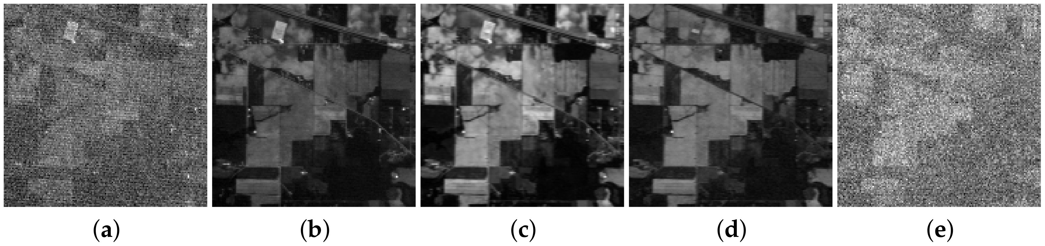
Figure 2.
Algorithm flow of the proposed method.

Figure 3.
Graphical illustration of the collaborative sparse unmixing method through variable splitting and augmented Lagrangian (CLSUnSAL).
Figure 3.
Graphical illustration of the collaborative sparse unmixing method through variable splitting and augmented Lagrangian (CLSUnSAL).

Figure 4.
Abundance maps of 5 endmembers estimated with different methods under Gaussian white noise with both pure and mixed regions having 75 × 75 pixels and 224 bands. From top to bottom: ground truth, SUnSAL (), CLSUnSAL (), CUSAL-SP (), SU-NLE () () and SU-NLE () ().
Figure 4.
Abundance maps of 5 endmembers estimated with different methods under Gaussian white noise with both pure and mixed regions having 75 × 75 pixels and 224 bands. From top to bottom: ground truth, SUnSAL (), CLSUnSAL (), CUSAL-SP (), SU-NLE () () and SU-NLE () ().

Figure 5.
(a) The signal-to-noise ratio (SNR) of different band of the generated hyperspectral image (HSI) and (b) diagonal elements of the weighting matrix using proposed sparse unmixing method based on noise level estimation (SU-NLE) in simulated experiment I.
Figure 5.
(a) The signal-to-noise ratio (SNR) of different band of the generated hyperspectral image (HSI) and (b) diagonal elements of the weighting matrix using proposed sparse unmixing method based on noise level estimation (SU-NLE) in simulated experiment I.
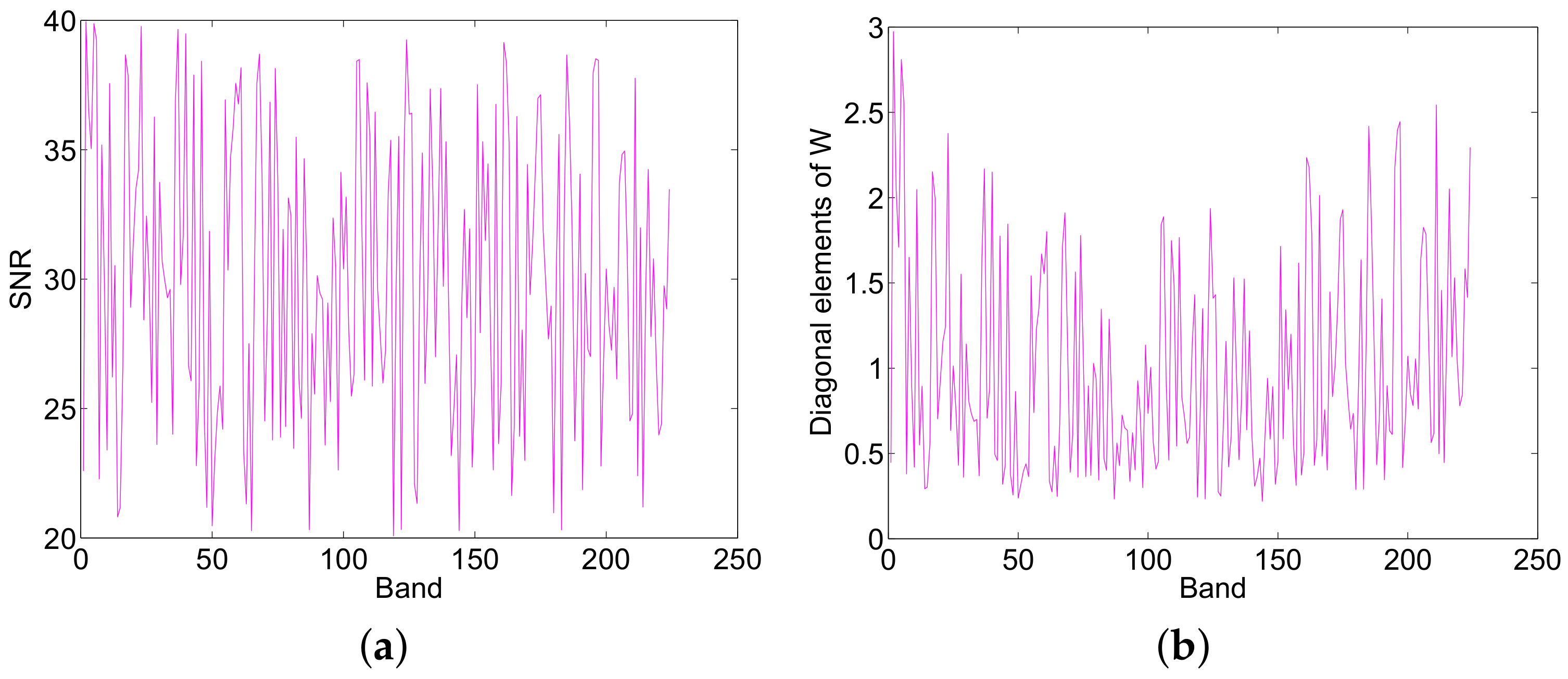
Figure 6.
SREs of the methods SU-NLE, SUnSAL and CLSUnSAL as a function of varying regularization parameter under Gaussian white noise with both pure and mixed regions having 75 × 75 pixels and 224 bands.
Figure 6.
SREs of the methods SU-NLE, SUnSAL and CLSUnSAL as a function of varying regularization parameter under Gaussian white noise with both pure and mixed regions having 75 × 75 pixels and 224 bands.
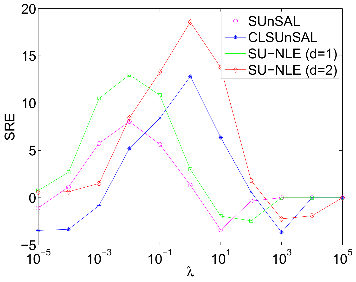
Figure 7.
Abundance maps of four endmembers estimated with different methods under Gaussian white noise with only mixed regions having 64 × 64 pixels and 224 bands. From top to bottom: ground truth, SUnSAL (), CLSUnSAL (), CUSAL-SP (), SU-NLE () () and SU-NLE () ().
Figure 7.
Abundance maps of four endmembers estimated with different methods under Gaussian white noise with only mixed regions having 64 × 64 pixels and 224 bands. From top to bottom: ground truth, SUnSAL (), CLSUnSAL (), CUSAL-SP (), SU-NLE () () and SU-NLE () ().
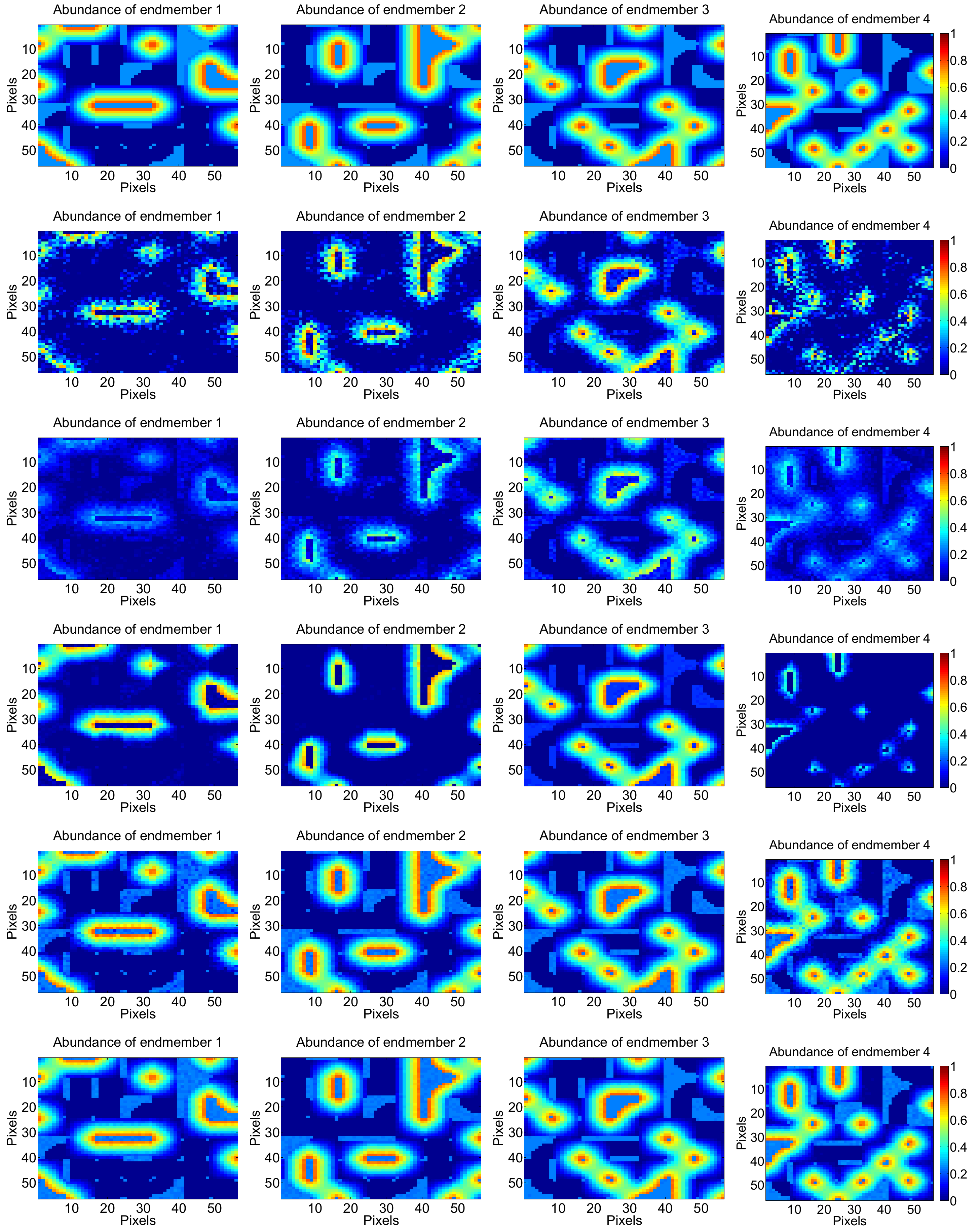
Figure 8.
(a) The SNR of different band of the generated HSI and (b) diagonal elements of the weighting matrix using proposed SU-NLE in simulated experiment II.
Figure 8.
(a) The SNR of different band of the generated HSI and (b) diagonal elements of the weighting matrix using proposed SU-NLE in simulated experiment II.

Figure 9.
Signal-to-reconstruction errors (SREs) of the methods SU-NLE, SUnSAL and CLSUnSAL as a function of varying regularization parameter under Gaussian white noise with only mixed regions having 64 × 64 pixels, 4 endmembers and 224 bands.
Figure 9.
Signal-to-reconstruction errors (SREs) of the methods SU-NLE, SUnSAL and CLSUnSAL as a function of varying regularization parameter under Gaussian white noise with only mixed regions having 64 × 64 pixels, 4 endmembers and 224 bands.
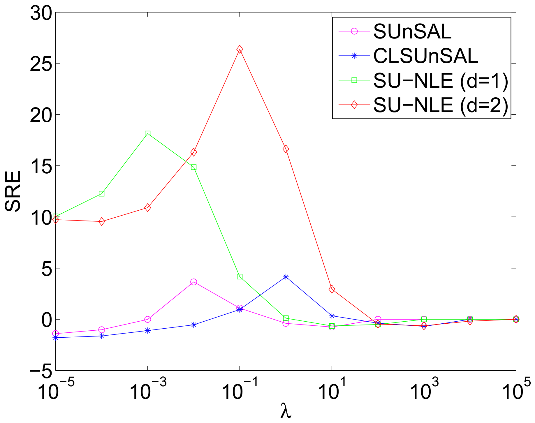
Figure 10.
SREs of different methods as a function of varying number of endmember under Gaussian white noise with only mixed regions having 64 × 64 pixels and 224 bands.
Figure 10.
SREs of different methods as a function of varying number of endmember under Gaussian white noise with only mixed regions having 64 × 64 pixels and 224 bands.

Figure 11.
SREs of different methods as a function of varying image size under Gaussian white noise with only mixed regions having 64 × 64 pixels, 4 endmembers and 224 bands.
Figure 11.
SREs of different methods as a function of varying image size under Gaussian white noise with only mixed regions having 64 × 64 pixels, 4 endmembers and 224 bands.

Figure 12.
Abundance maps of five endmembers estimated with different methods under correlated noise with both pure and mixed regions having 75 × 75 pixels and 224 bands. From top to bottom: ground truth, SUnSAL (), CLSUnSAL (), CUSAL-SP (), SU-NLE () () and SU-NLE () ().
Figure 12.
Abundance maps of five endmembers estimated with different methods under correlated noise with both pure and mixed regions having 75 × 75 pixels and 224 bands. From top to bottom: ground truth, SUnSAL (), CLSUnSAL (), CUSAL-SP (), SU-NLE () () and SU-NLE () ().

Figure 13.
(a) The SNR of different band of the generated HSI and (b) diagonal elements of the weighting matrix using proposed SU-NLE in simulated experiment III.
Figure 13.
(a) The SNR of different band of the generated HSI and (b) diagonal elements of the weighting matrix using proposed SU-NLE in simulated experiment III.
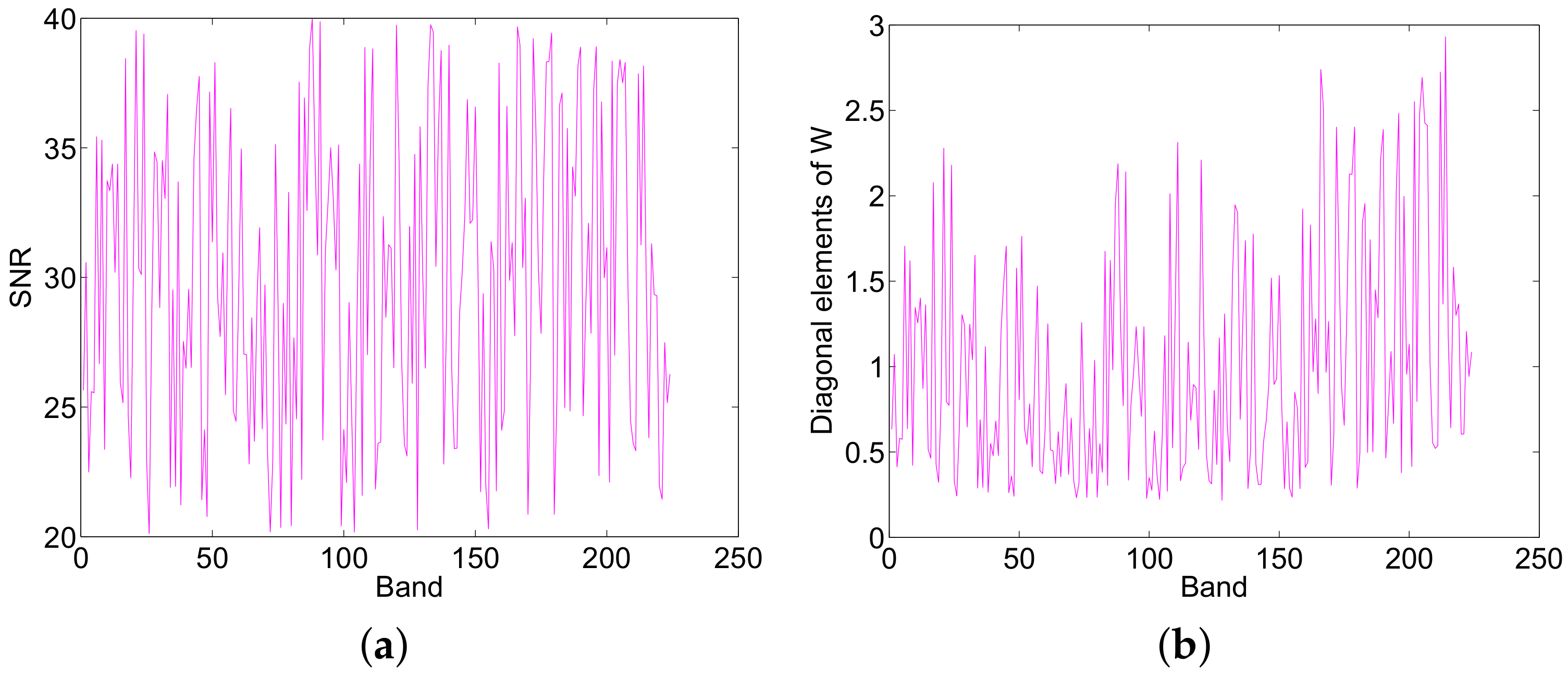
Figure 14.
SREs of the methods SU-NLE, SUnSAL and CLSUnSAL as a function of varying regularization parameter under correlated noise with both pure and mixed regions having 75 × 75 pixels and 224 bands.
Figure 14.
SREs of the methods SU-NLE, SUnSAL and CLSUnSAL as a function of varying regularization parameter under correlated noise with both pure and mixed regions having 75 × 75 pixels and 224 bands.
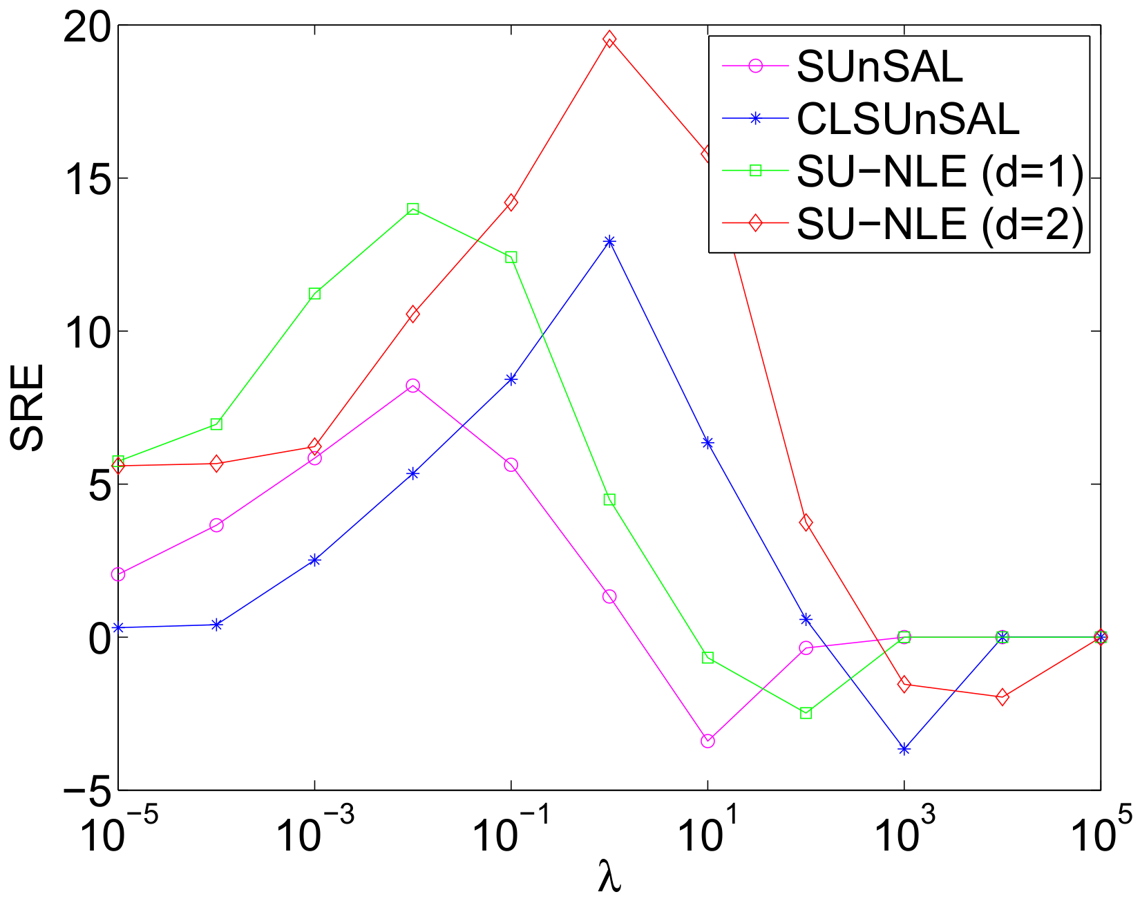
Figure 15.
Abundance maps of four endmembers estimated with different methods under correlated noise with only mixed regions having 64 × 64 pixels and 224 bands. From top to bottom: ground truth, SUnSAL (), CLSUnSAL (), CUSAL-SP (), SU-NLE () () and SU-NLE () ().
Figure 15.
Abundance maps of four endmembers estimated with different methods under correlated noise with only mixed regions having 64 × 64 pixels and 224 bands. From top to bottom: ground truth, SUnSAL (), CLSUnSAL (), CUSAL-SP (), SU-NLE () () and SU-NLE () ().

Figure 16.
(a) The SNR of different band of the generated HSI and (b) diagonal elements of the weighting matrix using proposed SU-NLE in simulated experiment IV.
Figure 16.
(a) The SNR of different band of the generated HSI and (b) diagonal elements of the weighting matrix using proposed SU-NLE in simulated experiment IV.

Figure 17.
SREs of the methods SU-NLE, SUnSAL and CLSUnSAL as a function of varying regularization parameter under correlated noise with only mixed regions having 64 × 64 pixels and 224 bands.
Figure 17.
SREs of the methods SU-NLE, SUnSAL and CLSUnSAL as a function of varying regularization parameter under correlated noise with only mixed regions having 64 × 64 pixels and 224 bands.

Figure 18.
SREs of different methods as a function of varying number of endmember under correlated noise with only mixed regions having 64 × 64 pixels and 224 bands.
Figure 18.
SREs of different methods as a function of varying number of endmember under correlated noise with only mixed regions having 64 × 64 pixels and 224 bands.

Figure 19.
SREs of different methods as a function of varying image size under correlated noise with only mixed regions having 64 × 64 pixels, 4 endmembers and 224 bands.
Figure 19.
SREs of different methods as a function of varying image size under correlated noise with only mixed regions having 64 × 64 pixels, 4 endmembers and 224 bands.
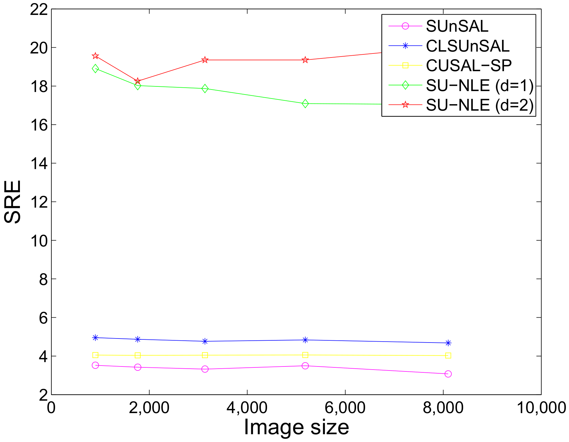
Figure 20.
False-color image of the AVIRIS Cuprite dataset.
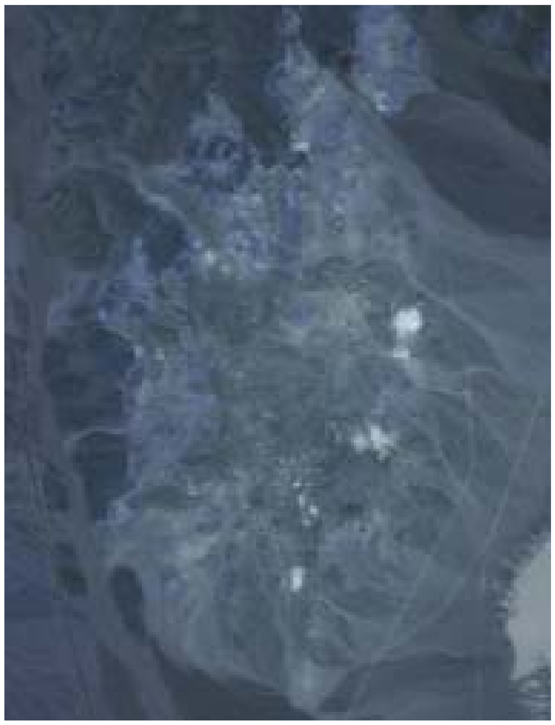
Figure 21.
United States Geological Survey (USGS) map of different minerals in the Cuprite mining district.
Figure 21.
United States Geological Survey (USGS) map of different minerals in the Cuprite mining district.

Figure 22.
The diagonal elements of weighting matrix for the real data.
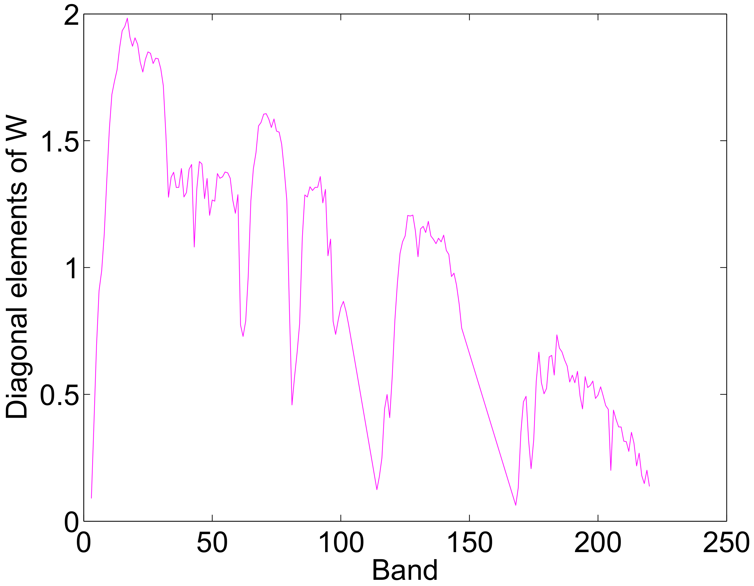
Figure 23.
Fractional abundance maps of three representative endmembers estimated by different unmixing methods using Cuprite dataset having pixels and 188 bands. From top to bottom: USGS Tetracorder classification map, SUnSAL (), CLSUnSAL (), CUSAL-SP (), SU-NLE () () and SU-NLE () ().
Figure 23.
Fractional abundance maps of three representative endmembers estimated by different unmixing methods using Cuprite dataset having pixels and 188 bands. From top to bottom: USGS Tetracorder classification map, SUnSAL (), CLSUnSAL (), CUSAL-SP (), SU-NLE () () and SU-NLE () ().


Table 1.
Common parameter setting of the proposed SU-NLE, SUnSAL and CLSUnSAL for synthetic data.
| Maxiter | |||
|---|---|---|---|
| {, , , , , 1, , , , , } | 1000 |
© 2017 by the authors. Licensee MDPI, Basel, Switzerland. This article is an open access article distributed under the terms and conditions of the Creative Commons Attribution (CC BY) license (http://creativecommons.org/licenses/by/4.0/).
Share and Cite
MDPI and ACS Style
Li, C.; Ma, Y.; Mei, X.; Fan, F.; Huang, J.; Ma, J. Sparse Unmixing of Hyperspectral Data with Noise Level Estimation. Remote Sens. 2017, 9, 1166. https://doi.org/10.3390/rs9111166
AMA Style
Li C, Ma Y, Mei X, Fan F, Huang J, Ma J. Sparse Unmixing of Hyperspectral Data with Noise Level Estimation. Remote Sensing. 2017; 9(11):1166. https://doi.org/10.3390/rs9111166
Chicago/Turabian StyleLi, Chang, Yong Ma, Xiaoguang Mei, Fan Fan, Jun Huang, and Jiayi Ma. 2017. "Sparse Unmixing of Hyperspectral Data with Noise Level Estimation" Remote Sensing 9, no. 11: 1166. https://doi.org/10.3390/rs9111166
Note that from the first issue of 2016, this journal uses article numbers instead of page numbers. See further details here.