Temporal and Spatial Comparison of Agricultural Drought Indices from Moderate Resolution Satellite Soil Moisture Data over Northwest Spain


Abstract
:
1. Introduction
2. Data and Methods
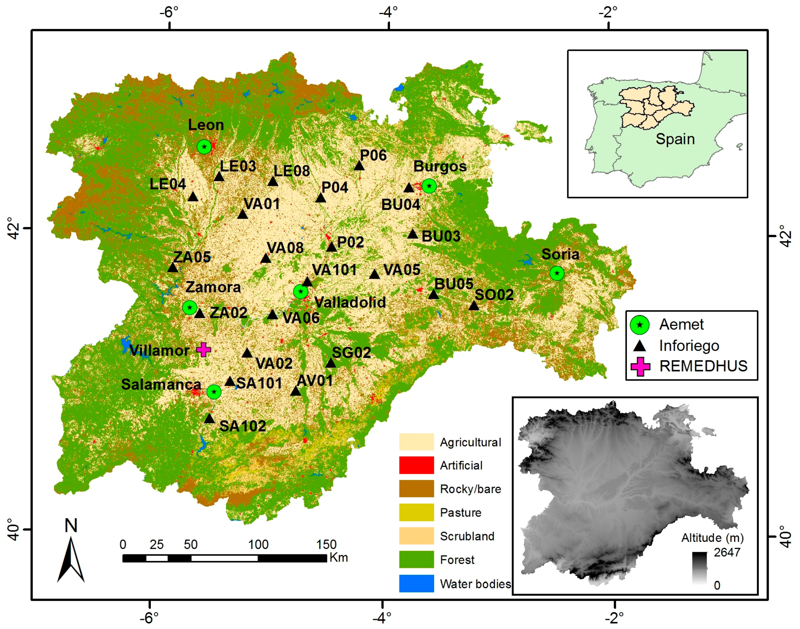
2.1. In Situ Data
2.2. Satellite Data
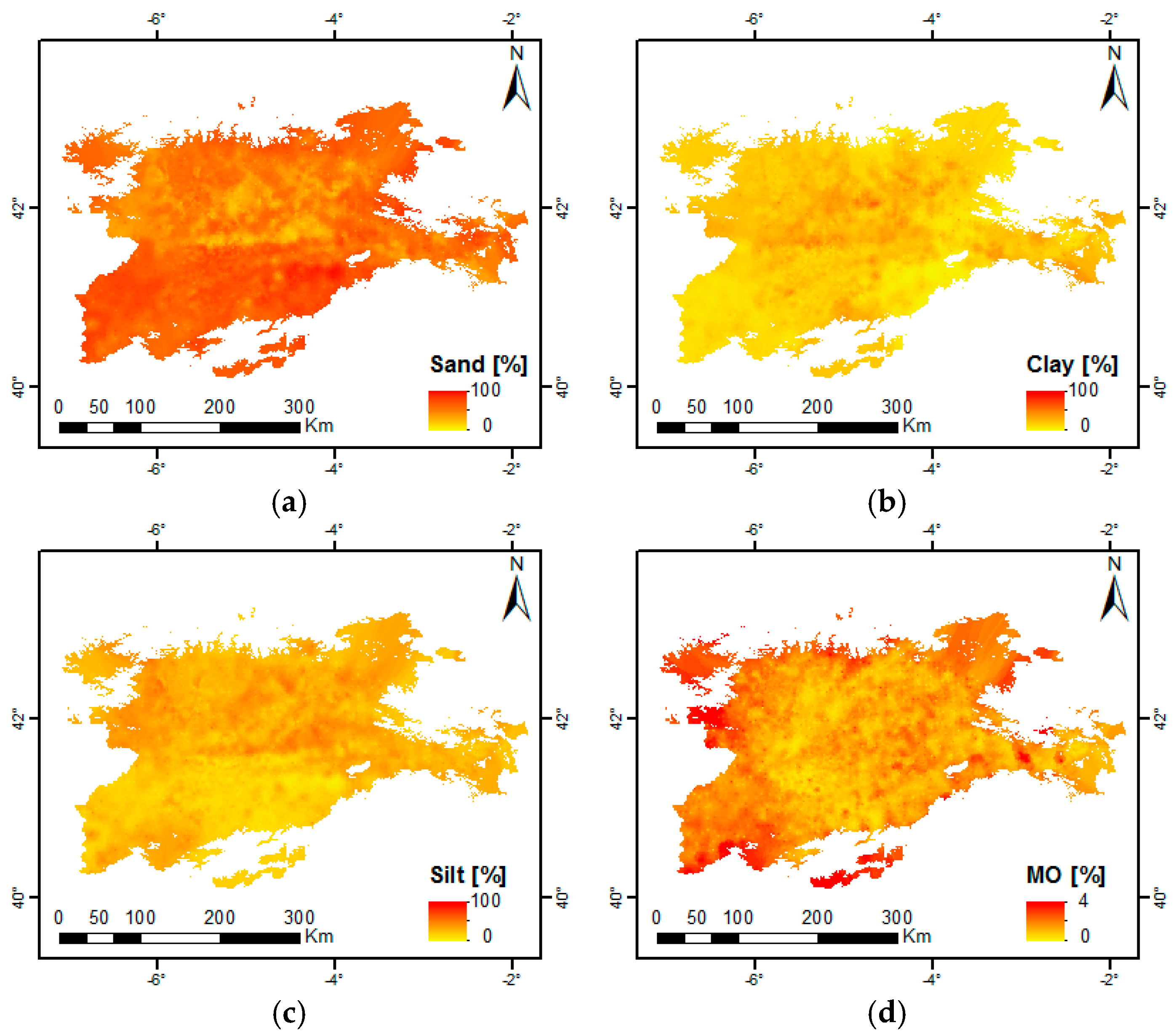
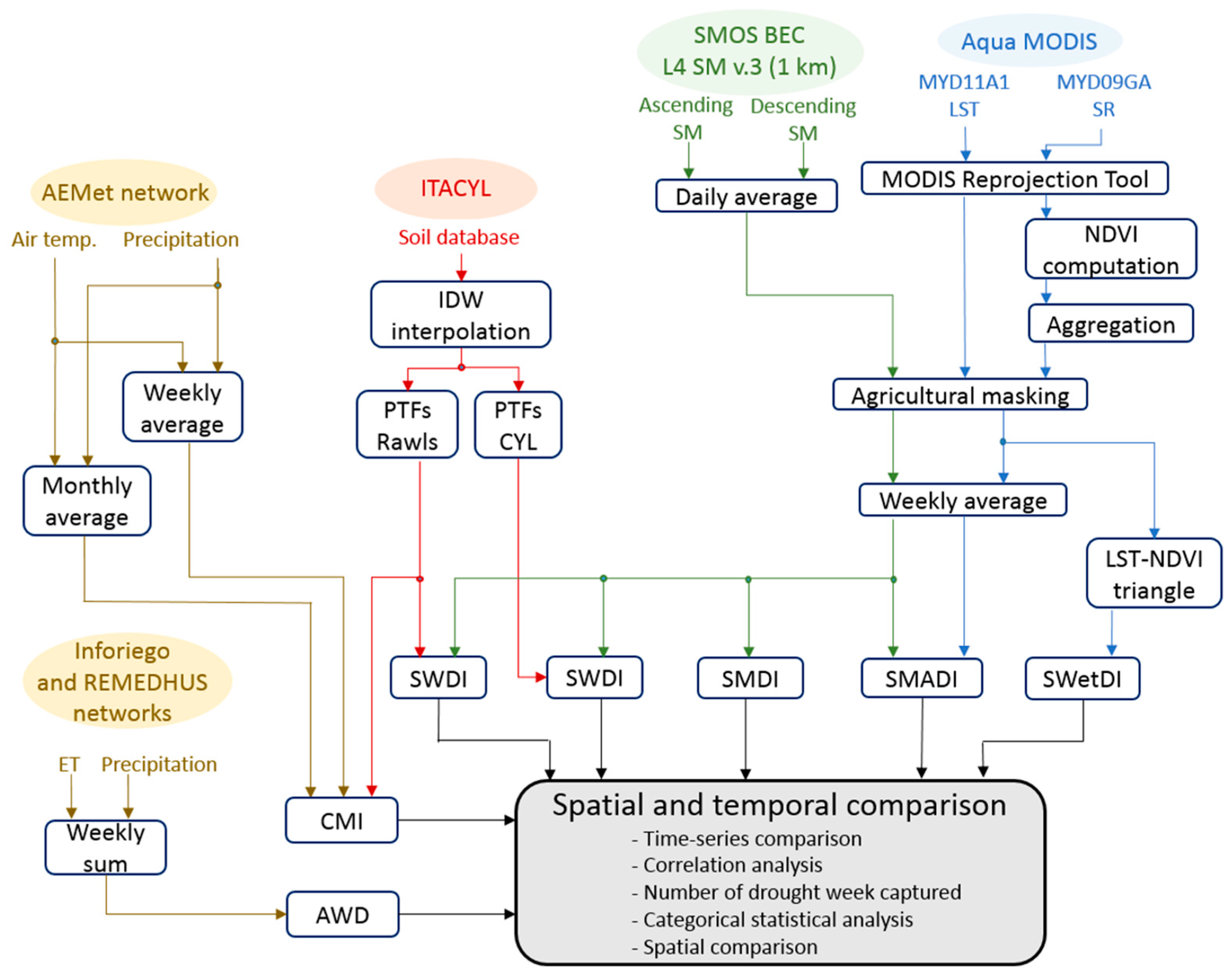
2.3. Data Processing
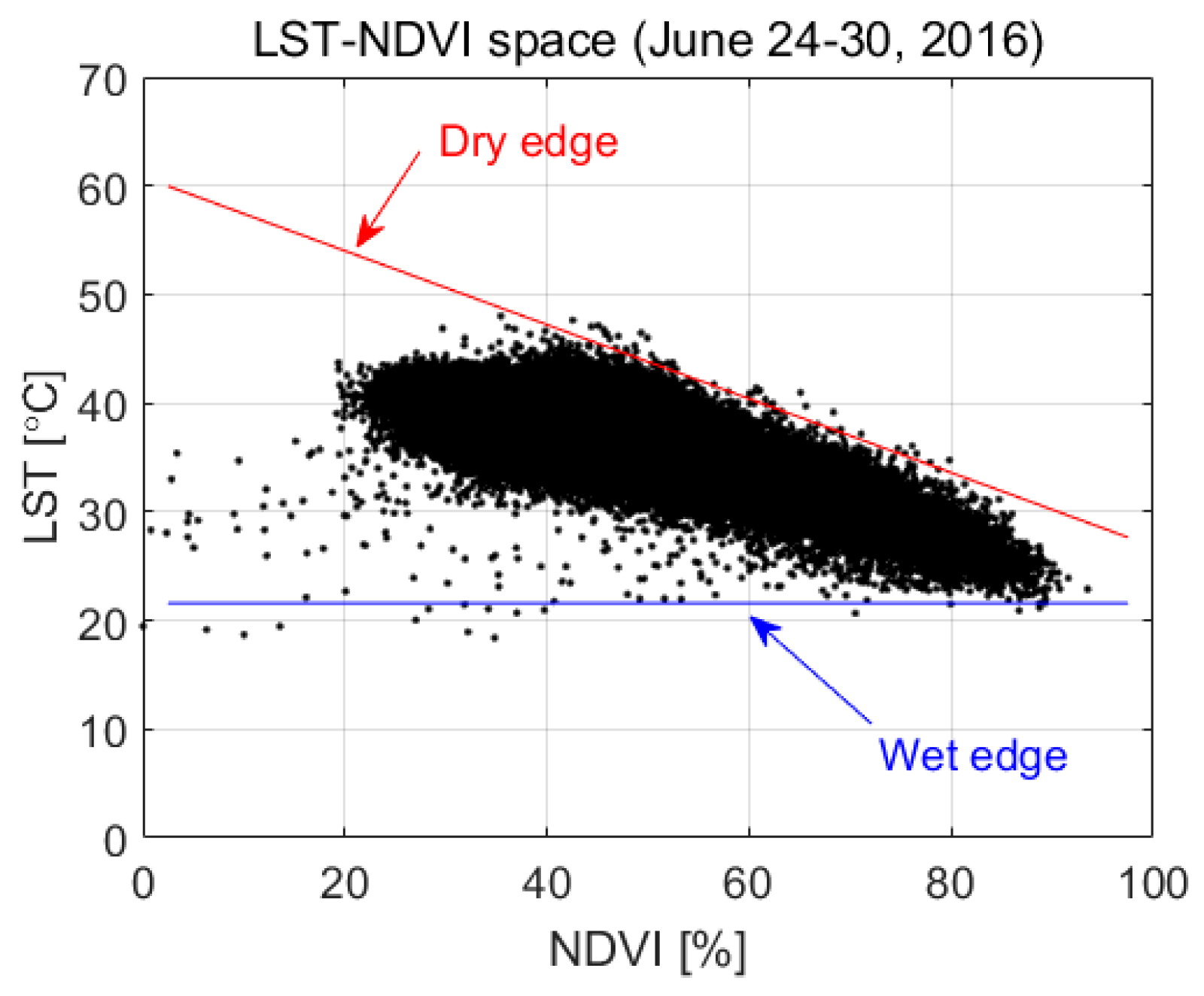
2.4. Estimation of Drought Indices
2.4.1. Atmospheric Water Deficit (AWD)
2.4.2. Crop Moisture Index (CMI)
2.4.3. Soil Water Deficit Index (SWDI)
2.4.4. Soil Moisture Agricultural Drought Index (SMADI)
2.4.5. Soil Moisture Deficit Index (SMDI)
2.4.6. Soil Wetness Deficit Index (SWetDI)
2.5. Comparison Strategy
3. Results and Discussion
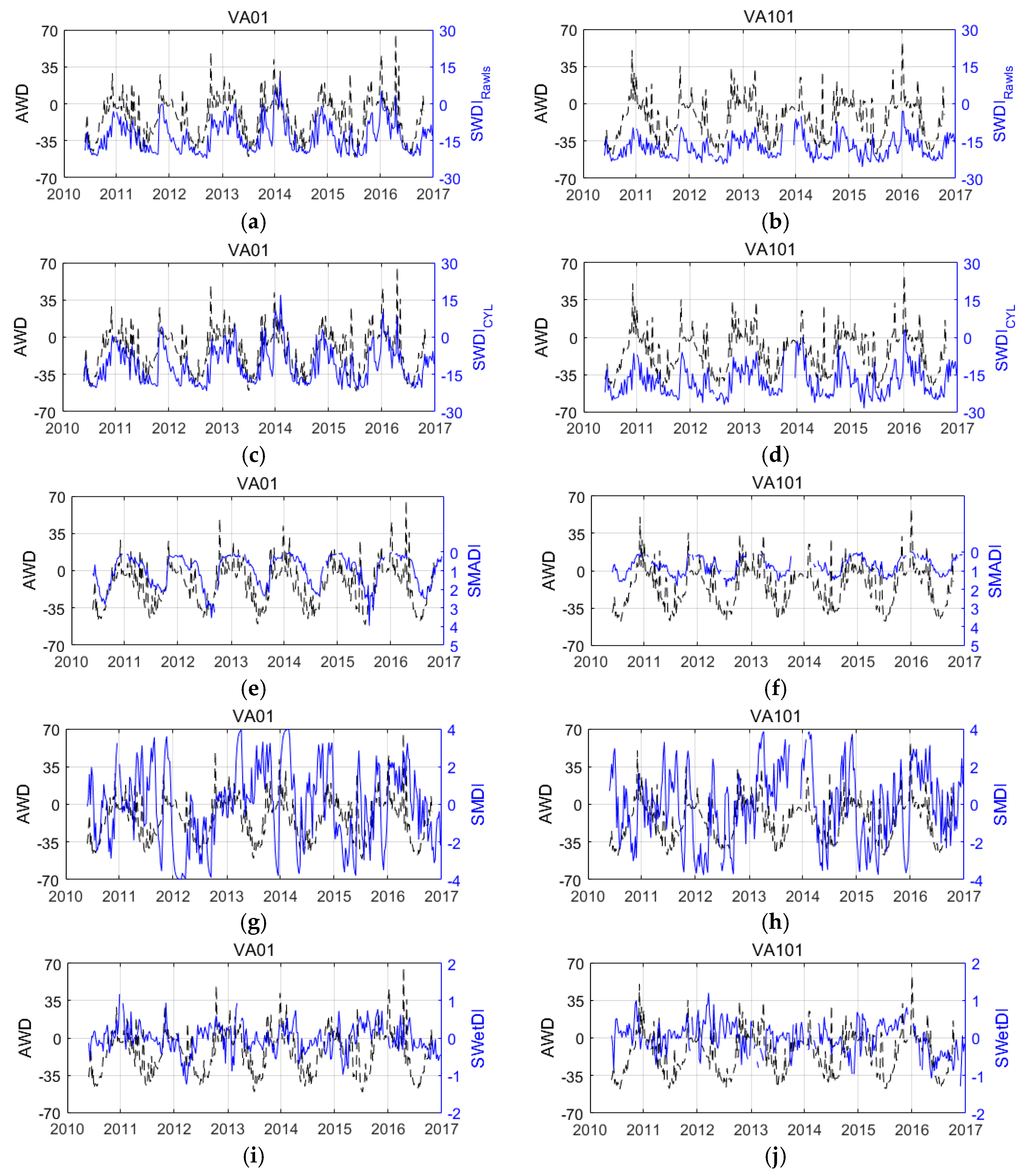
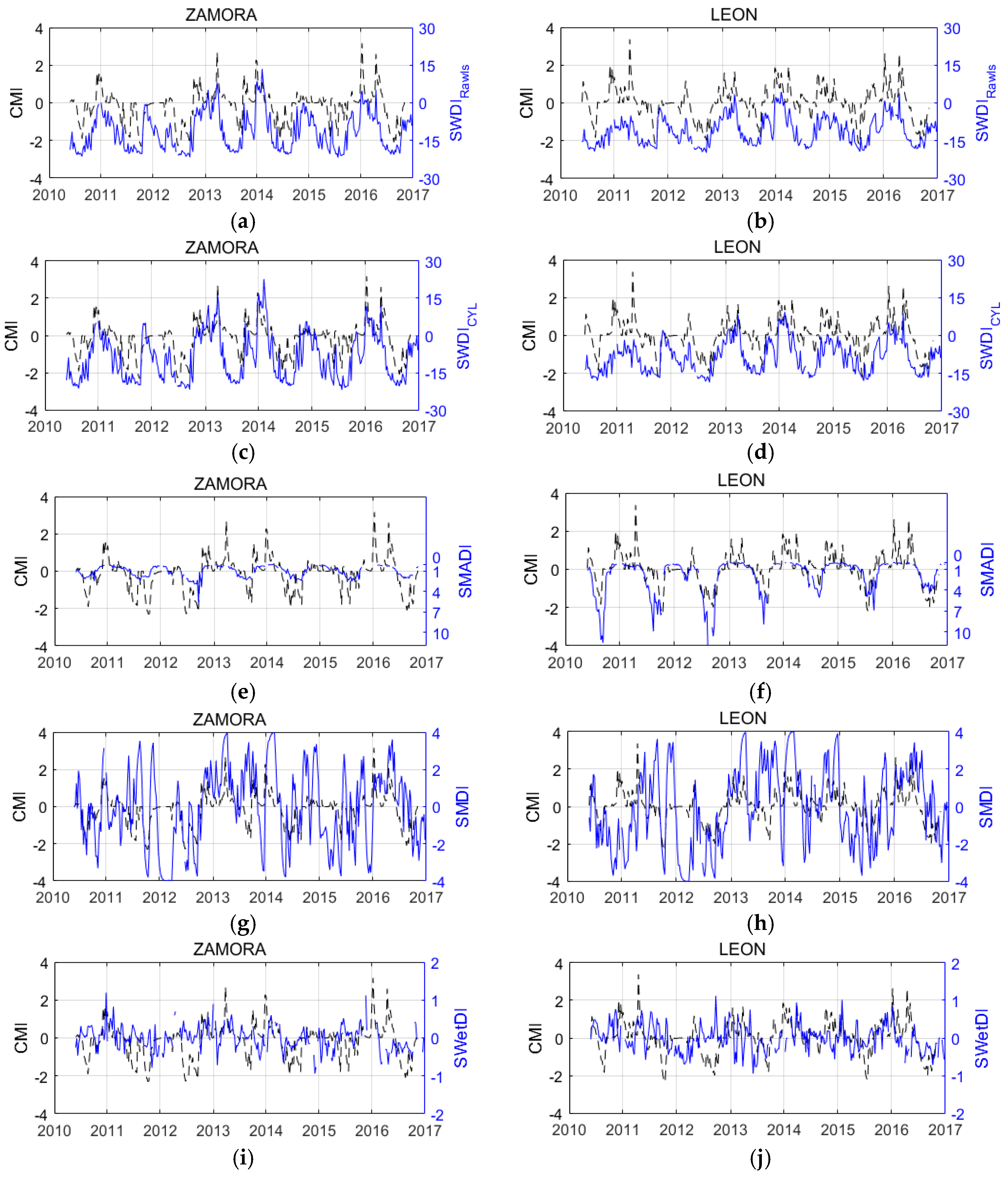
3.1. Time-Series Comparison
3.2. Correlation Analysis
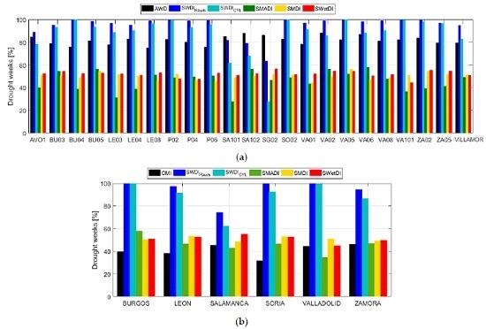
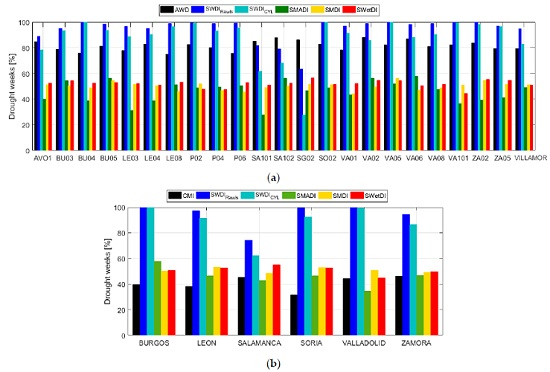
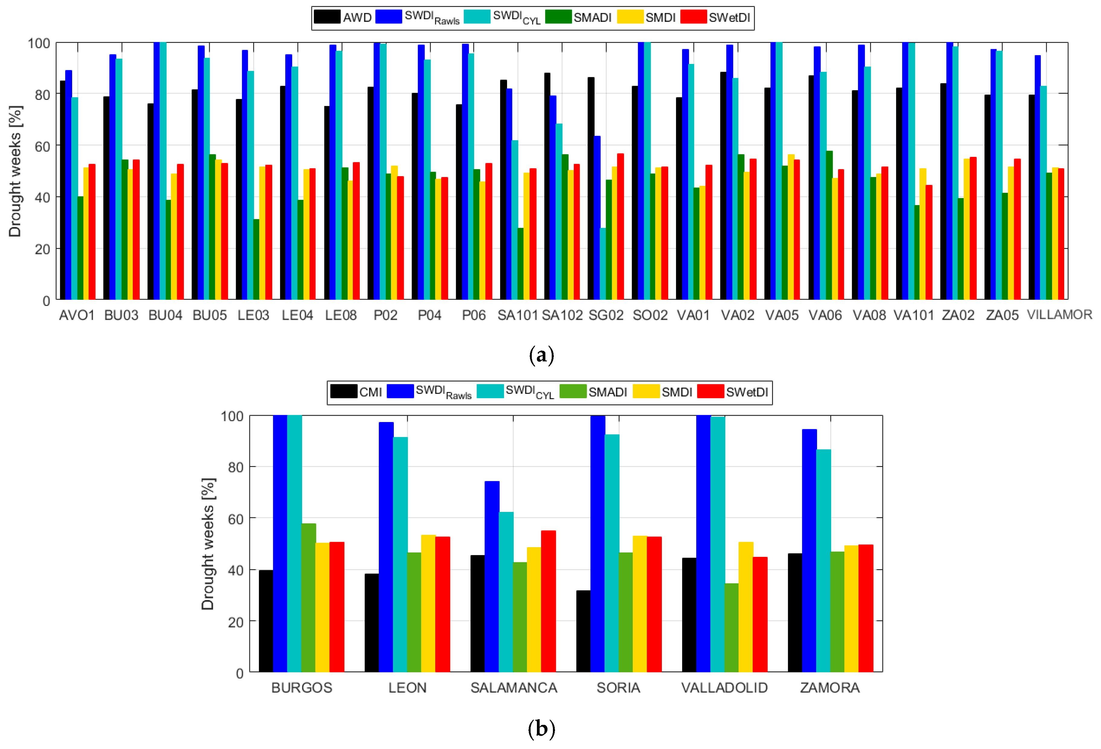
3.3. Drought Weeks Captured
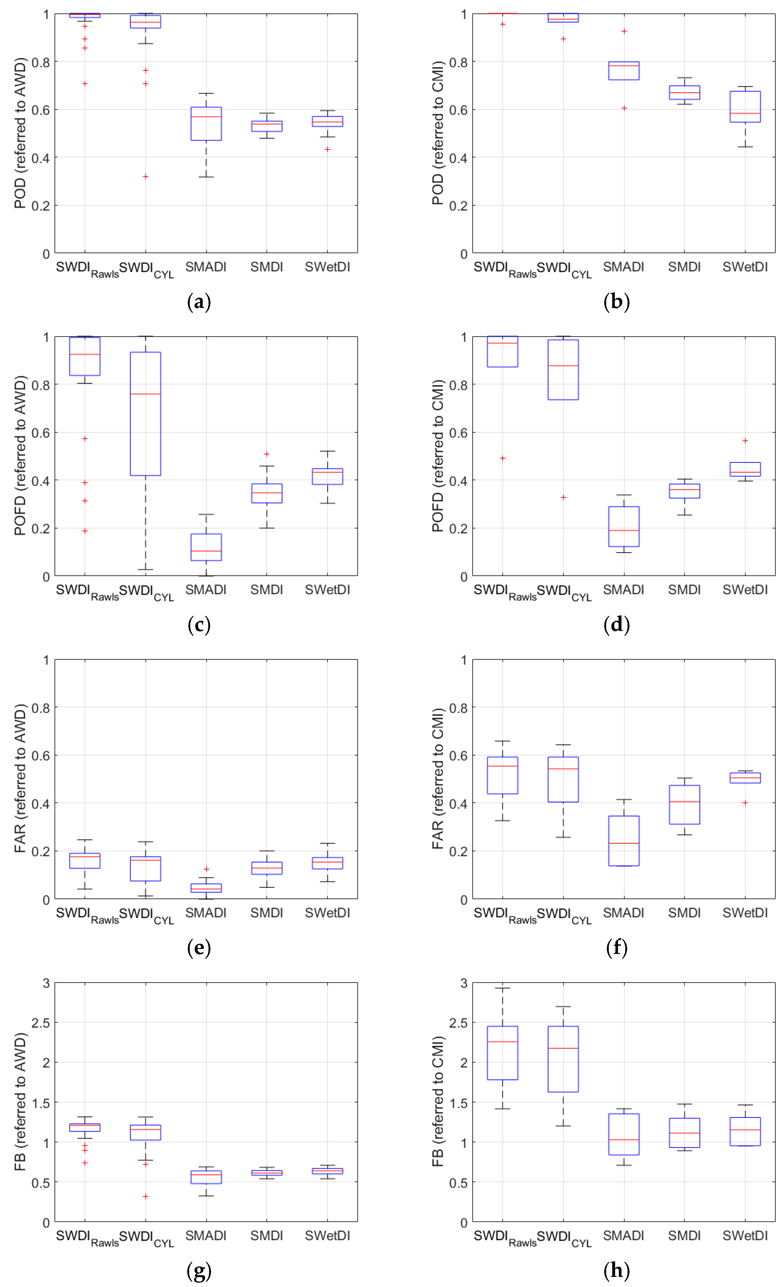
3.4. Categorical Statistical Analysis
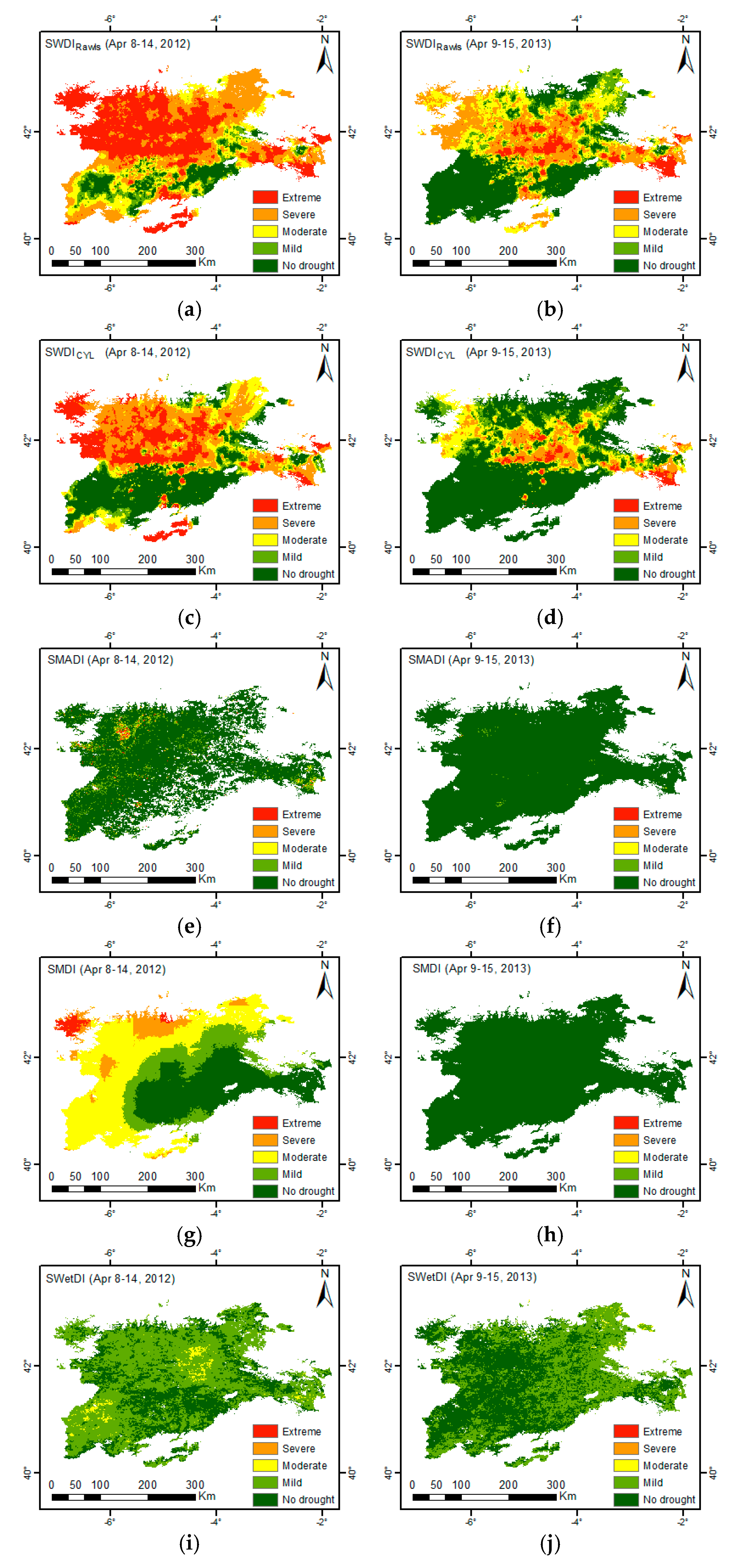
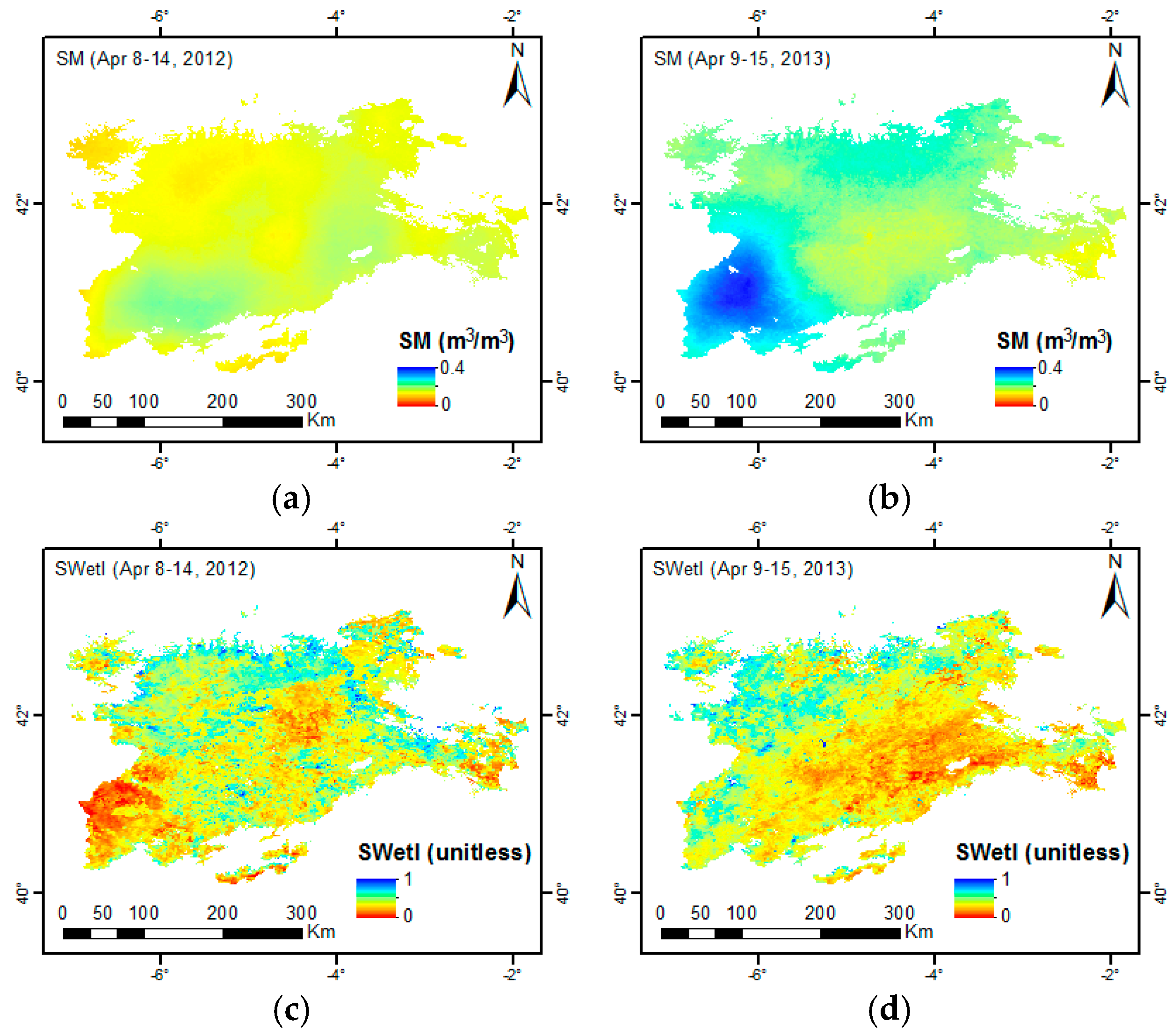
3.5. Spatial Comparison
4. Conclusions
Acknowledgments
Author Contributions
Conflicts of Interest
References
- FAO. Drought Characteristics and Management in the Caribbean; Food and Agriculture Organization of the United Nations (FAO): Rome, Italy, 2016; pp. 1–77. [Google Scholar]
- FAO. Horn of Africa Cross-Border Drought Action Plan 2017; Food and Agriculture Organization of the United Nations (FAO): Rome, Italy, 2017; pp. 1–12. [Google Scholar]
- Dracup, J.A.; Lee, K.S.; Paulson, E.G. On the statistical characteristics of drought events. Water Resour. Res. 1980, 16, 289–296. [Google Scholar] [CrossRef]
- Wilhite, D.A.; Glantz, M.H. Understanding: The drought phenomenon: The role of definitions. Water Int. 1985, 10, 111–120. [Google Scholar] [CrossRef]
- Wilhite, D.A. Drought as a Natural Hazard: Concepts and Definitions. In Drought: A Global Assessment; Wilhite, D.A., Ed.; Routledge: London, UK, 2000; Volume I, pp. 3–8. [Google Scholar]
- Heim, R.R.J. A Review of Twentieth-Century Drought Indices Used in the United States. Bull. Am. Meteorol. Soc. 2002, 83, 1149–1165. [Google Scholar]
- Panu, U.S.; Sharma, T. Challenges in drought research: Some perspectives and future directions. Hydrol. Sci. J. 2002, 47, S19–S30. [Google Scholar] [CrossRef]
- Quiring, S.M. Developing Objective Operational Definitions for Monitoring Drought. J. Appl. Meteorol. Climatol. 2009, 48, 1217–1229. [Google Scholar] [CrossRef]
- Mishra, A.K.; Singh, V.P. A review of drought concepts. J. Hydrol. 2010, 391, 202–216. [Google Scholar] [CrossRef]
- Zargar, A.; Sadiq, R.; Naser, B.; Khan, F.I. A review of drought indices. Environ. Rev. 2011, 19, 333–349. [Google Scholar] [CrossRef]
- McKee, T.B.; Doesken, N.J.; Kleist, J. The relationship of drought frequency and duration to time scales. In Proceedings of the 8th Conference on Applied Climatology, Anaheim, CA, USA, 17‒22 January 1993. [Google Scholar]
- Palmer, W.C. Meteorological Drought. In Research Paper No. 45; Connor, J.T., White, R.M., Eds.; U.S. Weather Bureau: Washington, DC, USA, 1965. [Google Scholar]
- Guttman, N.B.; Wallis, J.R.; Hosking, J.R.M. Spatial Comparability of the Palmer Drought Severity Index. J. Am. Water Resour. Assoc. 1992, 28, 1111–1119. [Google Scholar] [CrossRef]
- Wells, N.; Goddard, S.; Hayes, M.J. A Self-Calibrating Palmer Drought Severity Index. J. Clim. 2004, 17, 2335–2351. [Google Scholar] [CrossRef]
- Purcell, L.C.; Sinclair, T.R.; McNew, R.W. Drought Avoidance Assessment for Summer Annual Crops Using Long-Term Weather Data. Agron. J. 2003, 95, 1566–1576. [Google Scholar] [CrossRef]
- Torres, G.M.; Lollato, R.P.; Ochsner, T.E. Comparison of Drought Probability Assessments Based on Atmospheric Water Deficit and Soil Water Deficit. Agron. J. 2013, 105, 428–436. [Google Scholar] [CrossRef]
- Alley, W.M. The Palmer Drought Severity Index: Limitations and Assumptions. J. Clim. Appl. Meteorol. 1984, 23, 1100–1109. [Google Scholar] [CrossRef]
- Palmer, W.C. Keeping Track of Crop Moisture Conditions, Nationwide: The New Crop Moisture Index. Weatherwise 1968, 21, 156–161. [Google Scholar] [CrossRef]
- Karamouz, M.; Nazif, S.; Falahi, M. Hydrology and Hydroclimatology: Principles and Applications; Taylor and Francis Group, CRC Press: New York, NY, USA, 2012. [Google Scholar]
- Karl, T.R. The sensitivity of the Palmer drought severity index and Palmer’s Z-index to their calibration coefficients including potential evapotranspiration. J. Clim. Appl. Meteorol. 1986, 25, 77–86. [Google Scholar] [CrossRef]
- Shafer, B.A.; Dezman, L.E. Development of a surface water supply index (SWSI) to assess the severity of drought conditions in snowpack runoff areas. In Proceedings of the 50th Annual Western Snow Conference, Reno, NV, USA, 19‒23 April 1982. [Google Scholar]
- Svoboda, M.; Fuchs, B. Handbook of Drought Indicators and Indices; National Drought Mitigation Center: Lincoln, NE, USA, 2016. [Google Scholar]
- Seneviratne, S.I.; Corti, T.; Davin, E.L.; Hirschi, M.; Jaeger, E.B.; Lehner, I.; Orlowsky, B.; Teuling, A.J. Investigating soil moisture–climate interactions in a changing climate: A review. Earth-Sci. Rev. 2010, 99, 125–161. [Google Scholar] [CrossRef]
- Entekhabi, D.; Rodriguez-Iturbe, I.; Castelli, F. Mutual interaction of soil moisture state and atmospheric processes. J. Hydrol. 1996, 184, 3–17. [Google Scholar] [CrossRef]
- Keyantash, J.; Dracup, J.A. The Quantification of Drought: An Evaluation of Drought Indices. Bull. Am. Meteorol. Soc. 2002, 83, 1167–1180. [Google Scholar]
- Sheffield, J.; Goteti, G.; Wen, F.; Wood, E.F. A simulated soil moisture based drought analysis for the United States. J. Geophys. Res. Atmos. 2004, 109, D24. [Google Scholar] [CrossRef]
- Narasimhan, B.; Srinivasan, R. Development and evaluation of Soil Moisture Deficit Index (SMDI) and Evapotranspiration Deficit Index (ETDI) for agricultural drought monitoring. Agric. For. Meteorol. 2005, 133, 69–88. [Google Scholar] [CrossRef]
- Dutra, E.; Viterbo, P.; Miranda, P.M.A. ERA-40 reanalysis hydrological applications in the characterization of regional drought. Geophys. Res. Lett. 2008, 35. [Google Scholar] [CrossRef]
- Hao, Z.; AghaKouchak, A. Multivariate Standardized Drought Index: A parametric multi-index model. Adv. Water Resour. 2013, 57, 12–18. [Google Scholar] [CrossRef]
- Martínez-Fernández, J.; Ceballos, A.; Casado, S.; Morán, C.; Fernández, V. Runoff and soil moisture relationships in a small forested basin in the Sistema Central ranges (Spain). In Geomorphological Processes and Human Impacts in River Basins; Batalla, R.J., García, C., Eds.; International Association of Hidrological Sciences (IAHS) Press: Wallingford, UK, 2005; pp. 31–36. [Google Scholar]
- Sridhar, V.; Hubbard, K.G.; You, J.; Hunt, E.D. Development of the Soil Moisture Index to Quantify Agricultural Drought and Its “User Friendliness” in Severity-Area-Duration Assessment. J. Hydrometeorol. 2008, 9, 660–676. [Google Scholar] [CrossRef]
- Hunt, E.D.; Hubbard, K.G.; Wilhite, D.A.; Arkebauer, T.J.; Dutcher, A.L. The development and evaluation of a soil moisture index. Int. J. Climatol. 2009, 29, 747–759. [Google Scholar] [CrossRef]
- Martínez-Fernández, J.; González-Zamora, A.; Sánchez, N.; Gumuzzio, A. A soil water based index as a suitable agricultural drought indicator. J. Hydrol. 2015, 522, 265–273. [Google Scholar] [CrossRef]
- Ochsner, T.E.; Cosh, M.H.; Cuenca, R.H.; Dorigo, W.A.; Draper, C.S.; Hagimoto, Y.; Kerr, Y.H.; Njoku, E.G.; Small, E.E.; Zreda, M.; et al. State of the Art in Large-Scale Soil Moisture Monitoring. Soil Sci. Soc. Am. J. 2013, 77, 1888–1919. [Google Scholar] [CrossRef] [Green Version]
- Petropoulos, G.P.; Ireland, G.; Barrett, B. Surface soil moisture retrievals from remote sensing: Current status, products & future trends. Phys. Chem. Earth Parts A/B/C 2015, 83–84, 36–56. [Google Scholar]
- Mohanty, B.P.; Cosh, M.H.; Lakshmi, V.; Montzka, C. Soil Moisture Remote Sensing: State-of-the-Science. Vadose Zone J. 2017, 16. [Google Scholar] [CrossRef]
- Kerr, Y.H.; Al-Yaari, A.; Rodríguez-Fernández, N.; Parrens, M.; Molero, B.; Leroux, D.; Bircher, S.; Mahmoodi, A.; Mialon, A.; Richaume, P.; et al. Overview of SMOS performance in terms of global soil moisture monitoring after six years in operation. Remote Sens. Environ. 2016, 180, 40–63. [Google Scholar] [CrossRef]
- Al Bitar, A.; Mialon, A.; Kerr, Y.H.; Cabot, F.; Richaume, P.; Jacquette, E.; Quesney, A.; Mahmoodi, A.; Tarot, S.; Parrens, M.; et al. The global SMOS Level 3 daily soil moisture and brightness temperature maps. Earth Syst. Sci. Data 2017, 9, 293–315. [Google Scholar] [CrossRef]
- Chan, S.K.; Bindlish, R.; O’Neill, P.E.; Njoku, E.; Jackson, T.J.; Colliander, A.; Chen, F.; Burgin, M.; Dunbar, S.; Piepmeier, J.; et al. Assessment of the SMAP Passive Soil Moisture Product. IEEE Trans. Geosci. Remote Sens. 2016, 54, 4994–5007. [Google Scholar] [CrossRef]
- Colliander, A.; Jackson, T.J.; Bindlish, R.; Chan, S.; Das, N.; Kim, S.B.; Cosh, M.H.; Dunbar, R.S.; Dang, L.; Pashaian, L.; et al. Validation of SMAP surface soil moisture products with core validation sites. Remote Sens. Environ. 2017, 191, 215–231. [Google Scholar] [CrossRef]
- Kerr, Y.H.; Waldteufel, P.; Wigneron, J.P.; Delwart, S.; Cabot, F.; Boutin, J.; Escorihuela, M.J.; Font, J.; Reul, N.; Gruhier, C.; et al. The SMOS Mission: New Tool for Monitoring Key Elements of the Global Water Cycle. Proc. IEEE 2010, 98, 666–687. [Google Scholar] [CrossRef] [Green Version]
- Entekhabi, D.; Njoku, E.G.; O’Neill, P.E.; Kellogg, K.H.; Crow, W.T.; Edelstein, W.N.; Entin, J.K.; Goodman, S.D.; Jackson, T.J.; Johnson, J.; et al. The Soil Moisture Active Passive (SMAP) Mission. Proc. IEEE 2010, 98, 704–716. [Google Scholar] [CrossRef]
- Chung, D.; Dorigo, W.; De Jeu, R.; Kidd, R.; Wagner, W. Product Specification Document (PSD) D1.2.1 Version 1.9; ESA Climate Change Initiative Phase II-Soil Moisture; Earth Observation Data Centre for Water Resources Monitoring (EODC) GmbH: Vienna, Austria, 2017. [Google Scholar]
- Nghiem, S.V.; Wardlow, B.D.; Allured, D.; Svoboda, M.D.; LeComte, D.; Rosencrans, M.; Chan, S.K.; Neumann, G. Microwave Remote Sensing of Soil Moisture. In Remote Sensing of Drought: Innovative Monitoring Approaches; Wardlow, B.D., Anderson, M.C., Verdin, J.P., Eds.; Taylor & Francis Group: Boca Raton, FL, USA, 2012; pp. 197–226. [Google Scholar]
- Scaini, A.; Sánchez, N.; Vicente-Serrano, S.M.; Martínez-Fernández, J. SMOS-derived soil moisture anomalies and drought indices: A comparative analysis using in situ measurements. Hydrol. Process. 2015, 29, 373–383. [Google Scholar] [CrossRef]
- Martínez-Fernández, J.; González-Zamora, A.; Sánchez, N.; Gumuzzio, A.; Herrero-Jiménez, C.M. Satellite soil moisture for agricultural drought monitoring: Assessment of the SMOS derived Soil Water Deficit Index. Remote Sens. Environ. 2016, 177, 277–286. [Google Scholar] [CrossRef]
- Sánchez, N.; González-Zamora, A.; Piles, M.; Martínez-Fernández, J. A New Soil Moisture Agricultural Drought Index (SMADI) Integrating MODIS and SMOS Products: A Case of Study over the Iberian Peninsula. Remote Sens. 2016, 8, 287. [Google Scholar] [CrossRef]
- Martínez-Fernández, J.; González-Zamora, A.; Sánchez, N.; Pablos, M. CCI Soil Moisture for Long-Term Agricultural Drought Monitoring: A Case Study in Spain. In Proceedings of the IEEE International Geoscience and Remote Sensing Symposium (IGARSS), Fort Worth, TX, USA, 23–28 July 2017. [Google Scholar]
- Carrão, H.; Russo, S.; Sepulcre-Canto, G.; Barbosa, P. An empirical standardized soil moisture index for agricultural drought assessment from remotely sensed data. Int. J. Appl. Earth Obs. Geoinf. 2016, 48, 74–84. [Google Scholar] [CrossRef]
- Keshavarz, M.R.; Vazifedoust, M.; Alizadeh, A. Drought monitoring using a Soil Wetness Deficit Index (SWDI) derived from MODIS satellite data. Agric. Water Manag. 2014, 132, 37–45. [Google Scholar] [CrossRef]
- Mallick, K.; Bhattacharya, B.K.; Patel, N.K. Estimating volumetric surface moisture content for cropped soils using a soil wetness index based on surface temperature and NDVI. Agric. For. Meteorol. 2009, 149, 1327–1342. [Google Scholar] [CrossRef]
- Carlson, T. An Overview of the “Triangle Method” for Estimating Surface Evapotranspiration and Soil Moisture from Satellite Imagery. Sensors 2007, 7, 1612. [Google Scholar] [CrossRef]
- Stisen, S.; Sandholt, I.; Nørgaard, A.; Fensholt, R.; Jensen, K.H. Combining the triangle method with thermal inertia to estimate regional evapotranspiration—Applied to MSG-SEVIRI data in the Senegal River basin. Remote Sens. Environ. 2008, 112, 1242–1255. [Google Scholar] [CrossRef]
- Tang, R.; Li, Z.-L.; Tang, B. An application of the Ts–VI triangle method with enhanced edges determination for evapotranspiration estimation from MODIS data in arid and semi-arid regions: Implementation and validation. Remote Sens. Environ. 2010, 114, 540–551. [Google Scholar] [CrossRef]
- Tang, R.; Li, Z.L. An End-Member-Based Two-Source Approach for Estimating Land Surface Evapotranspiration From Remote Sensing Data. IEEE Trans. Geosci. Remote Sens. 2017, 55, 5818–5832. [Google Scholar] [CrossRef]
- Al Bitar, A.; Kerr, Y.H.; Merlin, O.; Cabot, F.; Wigneron, J.P. Global Drought Index from SMOS Soil Moisture. In Proceedings of the IEEE International Geoscience and Remote Sensing Symposium (IGARSS), Melbourne, Australia, 21–26 July 2013. [Google Scholar]
- Piles, M.; Camps, A.; Vall-llossera, M.; Corbella, I.; Panciera, R.; Rudiger, C.; Kerr, Y.H.; Walker, J. Downscaling SMOS-Derived Soil Moisture Using MODIS Visible/Infrared Data. IEEE Trans. Geosci. Remote Sens. 2011, 49, 3156–3166. [Google Scholar] [CrossRef]
- Merlin, O.; Rudiger, C.; Al Bitar, A.; Richaume, P.; Walker, J.P.; Kerr, Y.H. Disaggregation of SMOS Soil Moisture in Southeastern Australia. IEEE Trans. Geosci. Remote Sens. 2012, 50, 1556–1571. [Google Scholar] [CrossRef] [Green Version]
- Piles, M.; Sánchez, N.; Vall-llossera, M.; Camps, A.; Martínez-Fernández, J.; Martínez, J.; González-Gambau, V. A Downscaling Approach for SMOS Land Observations: Evaluation of High-Resolution Soil Moisture Maps Over the Iberian Peninsula. IEEE J. Sel. Top. Appl. Earth Obs. Remote Sens. 2014, 7, 3845–3857. [Google Scholar] [CrossRef]
- Sánchez-Ruiz, S.; Piles, M.; Sánchez, N.; Martínez-Fernández, J.; Vall-llossera, M.; Camps, A. Combining SMOS with visible and near/shortwave/thermal infrared satellite data for high resolution soil moisture estimates. J. Hydrol. 2014, 516, 273–283. [Google Scholar] [CrossRef]
- Merlin, O.; Malbéteau, Y.; Notfi, Y.; Bacon, S.; Khabba, S.E.R.; Jarlan, L. Performance Metrics for Soil Moisture Downscaling Methods: Application to DISPATCH Data in Central Morocco. Remote Sens. 2015, 7, 3783–3807. [Google Scholar] [CrossRef]
- Piles, M.; Petropoulos, G.P.; Sánchez, N.; González-Zamora, A.; Ireland, G. Towards improved spatio-temporal resolution soil moisture retrievals from the synergy of SMOS and MSG SEVIRI spaceborne observations. Remote Sens. Environ. 2016, 180, 403–417. [Google Scholar] [CrossRef]
- Pablos, M.; Piles, M.; Sánchez, N.; Vall-llossera, M.; Martínez-Fernández, J.; Camps, A. Impact of day/night time land surface temperature in soil moisture disaggregation algorithms. Eur. J. Remote Sens. 2016, 49, 899–916. [Google Scholar] [CrossRef]
- BEC-Team. Quality Report: Validation of SMOS-BEC L4 High Resolution Soil Moisture Products v.3; Barcelona Expert Centre (BEC): Barcelona, Spain, 2015. [Google Scholar]
- Portal, G.; Vall-llossera, M.; Piles, M.; Camps, A.; Chaparro, D.; Pablos, M.; Rossato, L. A Two-Scale Downscaling Approach for SMOS Using Adaptative Moving Windows. In Proceedings of the IEEE International Geoscience and Remote Sensing Symposium (IGARSS), Fort Worth, TX, USA, 23–28 July 2017. [Google Scholar]
- Sánchez, N.; Martinez-Fernández, J.; Scaini, A.; Pérez-Gutiérrez, C. Validation of the SMOS L2 Soil Moisture Data in the REMEDHUS Network (Spain). IEEE Trans. Geosci. Remote Sens. 2012, 50, 1602–1611. [Google Scholar] [CrossRef]
- González-Zamora, A.; Sánchez, N.; Martínez-Fernández, J.; Gumuzzio, A.; Piles, M.; Olmedo, E. Long-term SMOS soil moisture products: A comprehensive evaluation across scales and methods in the Duero Basin (Spain). Phys. Chem. Earth Parts A/B/C 2015, 83–84, 123–136. [Google Scholar] [CrossRef]
- Servicio de Estadística, Estudios y Planificación Agraria. La Agricultura y la Ganadería de Castilla y León en Cifras; Junta de Castilla y León, Ed.; Consejería de Agricultura y Ganadería: Valladolid, Spain, 2012. Available online: http://www.jcyl.es/web/jcyl/AgriculturaGanaderia/es/Plantilla100DetalleFeed/12464648 62173/Publicacion/1284287241442/Redaccion (accessed on 13 November 2017).
- Pablos, M.; Martínez-Fernández, J.; Piles, M.; Sánchez, N.; Vall-llossera, M.; Camps, A. Multi-Temporal Evaluation of Soil Moisture and Land Surface Temperature Dynamics Using in Situ and Satellite Observations. Remote Sens. 2016, 8, 587. [Google Scholar] [CrossRef]
- LP-DAAC. MODIS Reprojection Tool User’s Manual Release 4.1; USGS Earth Resources Observation and Science (EROS) Center: Sioux Falls, SD, USA, 2011.
- Allen, R.G.; Pereira, L.S.; Raes, D.; Smith, M. Crop Evapotranspiration: Guidelines for Computing Crop Water Requirements; Food and Agriculture Organization of the United Nations (FAO): Rome, Italy, 1998. [Google Scholar]
- Wells, N. PDSI Users Manual Version 2.0; National Agricultural Decision Support System (NADSS): Lincoln, NE, USA, 2003. [Google Scholar]
- Rawls, W.J.; Brakensiek, D.L.; Saxtonn, K.E. Estimation of Soil Water Properties. Trans. ASAE 1982, 25, 1316–1320. [Google Scholar] [CrossRef]
- Dumouchel, W.; O’Brien, F. Integrating a Robust Option into a Multiple Regression Computing Environment. In Computing and Graphics in Statistics; Buja, A., Tukey, P.A., Eds.; Springer New York, Inc.: New York, NY, USA, 1991; pp. 41–48. [Google Scholar]
- Ji, L.; Peters, A.J. Assessing vegetation response to drought in the northern Great Plains using vegetation and drought indices. Remote Sens. Environ. 2003, 87, 85–98. [Google Scholar] [CrossRef]
- Caccamo, G.; Chisholm, L.A.; Bradstock, R.A.; Puotinen, M.L. Assessing the sensitivity of MODIS to monitor drought in high biomass ecosystems. Remote Sens. Environ. 2011, 115, 2626–2639. [Google Scholar] [CrossRef]
- Sánchez, N.; González-Zamora, A.; Martínez-Fernández, J.; Piles, M.; Pablos, M.; Wardlow, B.; Tadesse, T.; Svoboda, M.D. Preliminary Assessment of an Integrated SMOS and MODIS Application for Global Agricultural Drought Monitoring. In Proceedings of the IEEE International Geoscience and Remote Sensing Symposium (IGARSS), Fort Worth, TX, USA, 23–28 July 2017. [Google Scholar]
- Paredes-Trejo, F.; Barbosa, H. Evaluation of the SMOS-Derived Soil Water Deficit Index as Agricultural Drought Index in Northeast of Brazil. Water 2017, 9, 377. [Google Scholar] [CrossRef]
- Mishra, A.; Vu, T.; Veettil, A.V.; Entekhabi, D. Drought monitoring with soil moisture active passive (SMAP) measurements. J. Hydrol. 2017, 552, 620–632. [Google Scholar] [CrossRef]
- McBride, J.L.; Ebert, E.E. Verification of Quantitative Precipitation Forecasts from Operational Numerical Weather Prediction Models over Australia. Weather. Forecast. 2000, 15, 103–121. [Google Scholar] [CrossRef]
- Toté, C.; Patricio, D.; Boogaard, H.; van der Wijngaart, R.; Tarnavsky, E.; Funk, C. Evaluation of Satellite Rainfall Estimates for Drought and Flood Monitoring in Mozambique. Remote Sens. 2015, 7, 1758. [Google Scholar] [CrossRef]
- Wilks, D.S. Statistical Methods in the Atmospheric Sciences, 3rd ed.; Academic Press: Oxford, UK, 2011; Volume 100, p. 704. [Google Scholar]
- Trigo, R.M.; Añel, J.A.; Barriopedro, D.; García-Herrera, R.; Gimeno, L.; Nieto, R.; Castillo, R.; Allen, M.R.; Massey, N. The record winter drought of 2011–12 in the Iberian Peninsula. Bull. Am. Meteorol. Soc. 2013, 94, S41. [Google Scholar]
- Di, L.; Rundquist, D.C.; Han, L. Modelling relationships between NDVI and precipitation during vegetative growth cycles. Int. J. Remote Sens. 1994, 15, 2121–2136. [Google Scholar] [CrossRef]
- Nicholson, S.E.; Farrar, T.J. The influence of soil type on the relationships between NDVI, rainfall, and soil moisture in semiarid Botswana. I. NDVI response to rainfall. Remote Sens. Environ. 1994, 50, 107–120. [Google Scholar] [CrossRef]
- Reed, B.C.; Brown, J.F.; VanderZee, D.; Loveland, T.R.; Merchant, J.W.; Ohlen, D.O. Measuring phenological variability from satellite imagery. J. Veg. Sci. 1994, 5, 703–714. [Google Scholar] [CrossRef]
- Wang, J.; Price, K.P.; Rich, P.M. Spatial patterns of NDVI in response to precipitation and temperature in the central Great Plains. Int. J. Remote Sens. 2001, 22, 3827–3844. [Google Scholar] [CrossRef]
- Cheng, Q.; Zhou, Q.; Zhang, H.F.; Liu, F.G. Spatial disparity of NDVI response in vegetation growing season to climate change in the Three-River Headwaters Region. Ecol. Environ. Sci. 2010, 19, 1284–1289. [Google Scholar]
- Zhang, F.; Zhang, L.; Wang, X.; Hung, J. Detecting Agro-Droughts in Southwest of China Using MODIS Satellite Data. J. Integr. Agric. 2013, 12, 159–168. [Google Scholar] [CrossRef]
- Quiring, S.M.; Ganesh, S. Evaluating the utility of the Vegetation Condition Index (VCI) for monitoring meteorological drought in Texas. Agric. For. Meteorol. 2010, 150, 330–339. [Google Scholar] [CrossRef]
- Li, R.; Tsunekawa, A.; Tsubo, M. Index-based assessment of agricultural drought in a semi-arid region of Inner Mongolia, China. J. Arid Land 2014, 6, 3–15. [Google Scholar] [CrossRef]
- González-Zamora, A.; Sánchez, N.; Martínez-Fernández, J.; Wagner, W. Root-zone plant available water estimation using the SMOS-derived soil water index. Adv. Water Resour. 2016, 96, 339–353. [Google Scholar] [CrossRef]
- Reichle, R.H.; De Lannoy, G.J.M.; Liu, Q.; Ardizzone, J.V.; Colliander, A.; Conaty, A.; Crow, W.; Jackson, T.J.; Jones, L.A.; Kimball, J.S.; et al. Assessment of the SMAP Level-4 Surface and Root-Zone Soil Moisture Product Using In Situ Measurements. J. Hydrometeorol. 2017, 18, 2624–2645. [Google Scholar] [CrossRef]
- Liu, D.; Mishra, A.K.; Yu, Z.; Yang, C.; Konapala, G.; Vu, T. Performance of SMAP, AMSR-E and LAI for weekly agricultural drought forecasting over continental United States. J. Hydrol. 2017, 553, 88–104. [Google Scholar] [CrossRef]
- Sivakumar, M.V.K.; Stone, R.; Sntelhas, P.C.; Svoboda, M.D.; Omondi, P.; Sarkar, J.; Wardlow, B. Agricultural Drought Indices: Summary and Recommendations, Agricultural Drought Indices. In Proceedings of the WMO/UNISDR Expert Group Meeting on Agricultural Drought Indices, Murcia, Spain, 2–4 June 2010; Sivakumar, M.V.K., Motha, R.P., Wilhite, D.A., Wook, D.A., Eds.; World Meteorological Organization (WMO): Geneva, Switzerland, 2010; pp. 172–197. [Google Scholar]


| AWD | CMI | SWDI | SMADI | SMDI | SWetDI | ||
|---|---|---|---|---|---|---|---|
| Dynamic Range | −∞ to +∞ | −∞ to +∞ | −∞ to +∞ | 0 to +∞ | −4 to +4 | −4 to+ 4 | |
| No drought | 0 or more | 0 or more | 0 or more | 0 to 1 | 0 or more | 0 or more | |
| Drought | Mild | less than 0 | −2 to −0.01 | −2 to −0.01 | 1.01 to 2 | −1 to −0.01 | −1 to −0.01 |
| Moderate | −3 to −2.01 | −5 to −2.01 | 2.01 to 3 | −2 to −1.01 | −2 to −1.01 | ||
| Severe | less than −3 | −10 to −5.01 | 3.01 to 4 | −3 to −2.01 | −3 to −2.01 | ||
| Extreme | - | less than −10 | more than 4 | −4 to −3.01 | −4 to −3.01 | ||
| Categorical Statistic | Equation | Dynamic Range | Perfect Score |
|---|---|---|---|
| Probability of Detection (POD) | 0 to 1 | 1 | |
| Probability of False Detection (POFD) | 0 to 1 | 0 | |
| False Alarm Ratio (FAR) | 0 to 1 | 0 | |
| Frequency Bias (FB) | −∞ to +∞ | 1 |
| Station | SWDIRawls | SWDICYL | SMADI | SMDI | SWetDI |
|---|---|---|---|---|---|
| AV01 | 0.76 | 0.76 | −0.71 | 0.18 | 0.02 * |
| BU03 | 0.78 | 0.78 | −0.51 | 0.19 | 0.09 * |
| BU04 | 0.68 | 0.68 | −0.62 | 0.19 | 0.15 |
| BU05 | 0.76 | 0.76 | −0.51 | 0.18 | 0.14 |
| LE03 | 0.69 | 0.69 | −0.41 | 0.20 | 0.15 |
| LE04 | 0.71 | 0.71 | −0.19 | 0.20 | 0.06 * |
| LE08 | 0.78 | 0.78 | −0.50 | 0.28 | 0.14 |
| P02 | 0.74 | 0.74 | −0.55 | 0.20 | 0.11 * |
| P04 | 0.77 | 0.77 | −0.60 | 0.25 | 0.11 * |
| P06 | 0.71 | 0.71 | −0.40 | 0.24 | 0.05 * |
| SA101 | 0.74 | 0.74 | −0.61 | 0.20 | 0.08 * |
| SA102 | 0.78 | 0.78 | −0.53 | 0.19 | 0.08 * |
| SG02 | 0.74 | 0.74 | −0.77 | 0.16 | 0.11 * |
| SO02 | 0.79 | 0.79 | −0.62 | 0.17 | 0.13 |
| VA01 | 0.80 | 0.80 | −0.72 | 0.24 | 0.15 |
| VA02 | 0.77 | 0.77 | −0.64 | 0.20 | 0.09 * |
| VA05 | 0.80 | 0.80 | −0.68 | 0.17 | 0.11 * |
| VA06 | 0.77 | 0.77 | −0.29 | 0.23 | 0.09 * |
| VA08 | 0.78 | 0.78 | −0.67 | 0.21 | 0.07 * |
| VA101 | 0.75 | 0.75 | −0.83 | 0.14 | 0.00 * |
| ZA02 | 0.77 | 0.77 | −0.19 | 0.19 | 0.06 * |
| ZA05 | 0.75 | 0.75 | −0.67 | 0.22 | 0.13 |
| VILLAMOR | 0.79 | 0.79 | −0.69 | 0.26 | 0.12 * |
| Station | SWDIRawls | SWDICYL | SMADI | SMDI | SWetDI |
|---|---|---|---|---|---|
| BURGOS | 0.60 | 0.60 | −0.58 | 0.44 | 0.25 |
| LEÓN | 0.69 | 0.69 | −0.61 | 0.39 | 0.19 |
| SALAMANCA | 0.66 | 0.66 | −0.57 | 0.40 | 0.08 * |
| SORIA | 0.48 | 0.48 | −0.54 | 0.41 | 0.28 |
| VALLADOLID | 0.70 | 0.70 | −0.32 | 0.42 | 0.07 * |
| ZAMORA | 0.69 | 0.69 | −0.69 | 0.44 | 0.13 |
© 2017 by the authors. Licensee MDPI, Basel, Switzerland. This article is an open access article distributed under the terms and conditions of the Creative Commons Attribution (CC BY) license (http://creativecommons.org/licenses/by/4.0/).
Share and Cite
Pablos, M.; Martínez-Fernández, J.; Sánchez, N.; González-Zamora, Á. Temporal and Spatial Comparison of Agricultural Drought Indices from Moderate Resolution Satellite Soil Moisture Data over Northwest Spain. Remote Sens. 2017, 9, 1168. https://doi.org/10.3390/rs9111168
Pablos M, Martínez-Fernández J, Sánchez N, González-Zamora Á. Temporal and Spatial Comparison of Agricultural Drought Indices from Moderate Resolution Satellite Soil Moisture Data over Northwest Spain. Remote Sensing. 2017; 9(11):1168. https://doi.org/10.3390/rs9111168
Chicago/Turabian StylePablos, Miriam, José Martínez-Fernández, Nilda Sánchez, and Ángel González-Zamora. 2017. "Temporal and Spatial Comparison of Agricultural Drought Indices from Moderate Resolution Satellite Soil Moisture Data over Northwest Spain" Remote Sensing 9, no. 11: 1168. https://doi.org/10.3390/rs9111168