Ionospheric Reconstructions Using Faraday Rotation in Spaceborne Polarimetric SAR Data
by
Cheng Wang
1,*, 
Liang Chen
1,
Haisheng Zhao
2,
Zheng Lu
3,
Mingming Bian
3,
Running Zhang
3 and
Jian Feng
2 1
Qian Xuesen Laboratory of Space Technology, China Academy of Space Technology, Beijing 100094, China
2
National Key Laboratory of Electromagnetic Environment, China Research Institute of Radiowave Propagation, Qingdao 266107, China
3
Beijing Institute of Spacecraft System Engineering, China Academy of Space Technology, Beijing 100094, China
*
Author to whom correspondence should be addressed.
Remote Sens. 2017, 9(11), 1169; https://doi.org/10.3390/rs9111169
Submission received: 3 August 2017
/
Revised: 11 November 2017
/
Accepted: 13 November 2017
/
Published: 14 November 2017
(This article belongs to the Special Issue Advances in SAR: Sensors, Methodologies, and Applications)
Abstract
:It is well known that the Faraday rotation (FR) is obviously embedded in spaceborne polarimetric synthetic aperture radar (PolSAR) data at L-band and lower frequencies. By model inversion, some widely used FR angle estimators have been proposed for compensation and provide a new field in high-resolution ionospheric soundings. However, as an integrated product of electron density and the parallel component of the magnetic field, FR angle measurements/observations demonstrate the ability to characterize horizontal ionosphere. In order to make a general study of ionospheric structure, this paper reconstructs the electron density distribution based on a modified two-dimensional computerized ionospheric tomography (CIT) technique, where the FR angles, rather than the total electron content (TEC), are regarded as the input. By using the full-pol (full polarimetric) data of Phase Array L-band Synthetic Aperture Radar (PALSAR) on board Advanced Land Observing Satellite (ALOS), International Reference Ionosphere (IRI) and International Geomagnetic Reference Field (IGRF) models, numerical simulations corresponding to different FR estimators and SAR scenes are made to validate the proposed technique. In simulations, the imaging of kilometer-scale ionospheric disturbances, a spatial scale that is rarely detectable by CIT using GPS, is presented. In addition, the ionospheric reconstruction using SAR polarimetric information does not require strong point targets within a SAR scene, which is necessary for CIT using SAR imaging information. Finally, the effects of system errors including noise, channel imbalance and crosstalk on the reconstruction results are also analyzed to show the applicability of CIT based on spaceborne full-pol SAR data.
1. Introduction
Due to the dispersive nature of ionosphere and the existence of Earth’s magnetic field, the polarization rotation of a linearly polarized wave will occur after traveling through the ionosphere. This phenomenon is known as Faraday rotation (FR) and depends on the frequency, the electron density, the Earth’s magnetic field, and the geometry of observation [1]. For spaceborne polarimetric synthetic aperture radar (PolSAR) systems at L-band and lower frequencies, FR will distort the scattering matrix (i.e., complex backscattering coefficients in the four channels of PolSAR) and become a significant error source [2]. Thus for a space-borne PolSAR system, some mitigation techniques are required.
It is known that the key in mitigation techniques is retrieval of the accurate FR angle by measuring the polluted scattering matrix. On the other hand, the FR retrieval from space using PolSAR is also a new capability of high-resolution ionospheric sounding, and various FR estimators have been proposed. After the transformation from Cartesian linear polarization to circular polarization, Bickel and Bates [3] propose a widely used FR estimator. The scattering matrix can be converted to the covariance matrix. By measuring the covariance matrix, one FR estimator is proposed by Freeman [2]. Chen and Quegan [4] propose six further FR estimators based on the off-diagonal terms of covariance matrix. It is important to note that none of above estimators is insensitive to all system errors (i.e., system noise, channel phase/amplitude imbalance, and crosstalk) and scattering types in SAR scenes. For example, the Chen and Quegan’s third estimator is the preferred one to channel amplitude imbalance but worse than Bickel and Bates estimator when the channel phase imbalance is the dominant error [4]. As discussed by Rogers and Quegan [5], the performance of Chen and Quegan’s third estimator is scattering dependent. Thus, in order to obtain the accurate FR angle, the choice of FR estimator should depend on the domain error and scattering types.
Assume the magnetic field along the path is approximately equal to a median value; the vertical TEC (i.e., the integration of electron density) distribution with kilometer-scale in terms of latitude and longitude can further be obtained, which is clearly beneficial to the studies of small-scale ionospheric features [6,7,8,9,10,11]. However, the information of TEC distribution is still limited to the detection of ionospheric horizontal structure. Compared with TEC, the spatial distribution of electron density can give a better study of ionospheric inhomogeneity or irregularity caused by the magnetic storms, earthquakes, etc. [12,13,14,15]. Thus, the electron density reconstruction based on the computerized ionospheric tomography (CIT) technique is required. By setting a series of ground-based GPS (Global Positioning System) receivers, the CIT technique was proposed to reconstruct the electron density distribution [16,17]. The TEC values for different look angles can be retrieved from GPS signals and regarded as the input of CIT. However, it is only suitable for hundred kilometers scale electron density monitoring [13,14,15]. In order to improve the resolution, previous studies have considered the CIT based on the information of spaceborne SAR imaging [18,19,20]. After the signal has passed twice through the ionosphere, its linear frequency modulated (FM) rate will be changed [21]. An autofocus algorithm is applied here to iteratively search the change of FM rate, which can further be used to derive the TEC value [22]. Although it can provide a high resolution reconstruction, the autofocus algorithm is insensitivity to TEC because of the limitation of small bandwidth for current low-frequency spaceborne SAR systems, e.g., the ALOS Phase Array L-band Synthetic Aperture Radar (PALSAR) [23,24]. In addition, it also requires strong point targets with high signal-to-clutter (SCR) ratio in a SAR scene [22,25].
In contrast to the TEC retrieval based on SAR imaging information, the TEC derived from FR using polarimetric information is independent of above limitations [10,26,27]. Recently, we have reconstructed the ionosphere by using the TEC values derived from FR [28]. However, as discussed above, the TEC derived from FR will introduce the error that the magnetic field must be approximated by a fixed value. Thus, in order to avoid it, the CIT reconstruction based on spaceborne PolSAR will be a promising direction where the FR angles are directly regarded as the input. FR can be defined as the integration of electron density weighted by the magnetic field along the ray path. Since in most cases, the magnetic field distribution is known with high precision from the International Geomagnetic Reference Field (IGRF) model, this information can be used to realize the final reconstruction of electron density after modifying the traditional CIT technique. In addition, this paper also focuses on the systems errors on the proposed CIT reconstruction. We start with a brief review of the main FR estimators from the full-pol data in Section 2. By using the PALSAR full-pol data sets, International Reference Ionosphere (IRI) and IGRF models, a modified two-dimensional CIT technique based on the spaceborne PolSAR system is analyzed in Section 3. The effects of system errors on the reconstructions are analyzed in Section 4. In addition, the results based on different FR estimators are also compared. Last, our conclusions are presented in Section 5.
2. Review of FR Estimators Based on the Spaceborne PolSAR Data
Due to the existence of Earth’s magnetic field in the ionosphere, a linearly polarized wave will split into ordinary and extraordinary waves with different phase velocities. The linearly polarized wave is therefore rotated by an angle called FR after traveling through the ionosphere, and can be derived by the half integration of the phase difference along the ray path [1,29]
where is the angle between signal propagation direction and magnetic field, is the magnitude of magnetic field, is the electron density (unit is electrons·m−3), and is the frequency. We can see that is inversely proportional to the square of the frequency and depends on the , and along the path. For a full-pol SAR system at L-band or lower, all the linearly polarized waves in each channel will encounter the ionospheric effects. The measured scattering matrix can then be written as Rogers and Quegan [5]:
Here, , , and are the independent complex Gaussian noise in each measurement, , , and are the true scattering matrix, and denote the channel imbalance on receive and transmit, respectively and are the crosstalk on receive, and and are the crosstalk on transmit. In an ideal system, the noise and crosstalk are zero, and the channel imbalance is equal to 1, the covariance matrix can then be derived as follow as Freeman [2]
where and represent averaging and conjugate, respectively. By assuming reflection symmetry, Freeman [2] has proposed one FR estimator formulated as
where
and denotes the real part. According to the off-diagonal terms of Equation (3), Chen and Quegan [4] proposed six further FR estimators, where the third one performs the best. This estimator can be written as
where
and denotes the imaginary part. Bickel and Bates [3] note that, in the absence of system errors and assuming reciprocity, the scattering of Equation (2) can be transformed into a circular polarization basis, that is,
Thus, the FR estimated from Equation (8) can be written as
3. Principle of the Proposed CIT Using FR Angles
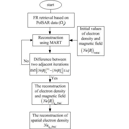
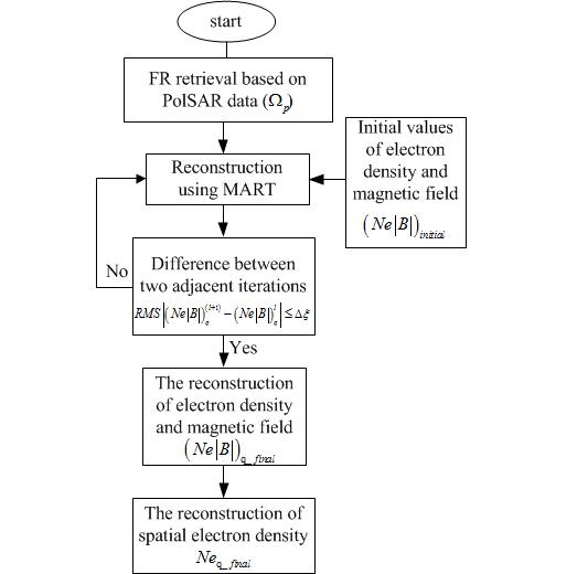
For the traditional CIT reconstruction, the TEC value is first retrieved and regarded as the input parameter. The well-known multiplicative algebraic reconstruction technique (MART) using iterative scheme is then applied to reconstruct the true electron density distribution [16,17,30]. In the iterative scheme of MART, the electron density distribution obtained from IRI model is used as the initial value. However, for the proposed CIT based on the spaceborne PolSAR data, the FR angle, rather than TEC value, is first retrieved and regarded as the input. Correspondingly, the spatial distribution of the product of electron density and the magnitude of magnetic field are used as the initial value in iteration.
The map of the proposed two-dimensional CIT technique is shown in Figure 1, where the annotations in red denote the main differences from traditional CIT due to the consideration of magnetic field [28]. The magnetic field varies in altitude and azimuth directions. The whole ionosphere region of interest is subdivided into H grids, where the product of electron density and magnetic field, rather than only electron density for traditional CIT, are constant in each grid. It is assumed that the whole synthetic aperture of PolSAR is divided into L sub-apertures and corresponding sampling position is located at the center of each sub-aperture. For traditional CIT simulations based on GPS [14,15,16,17], a set of ground-based receiver stations are required. At each sampling position of GPS, different TEC values corresponding to different receiver stations can then be obtained. From Figure 1, the explored ground scene is divided into K subimages, which is similar to the ground-based receiver. At one sub-aperture, by applying averaging within each subimage, the distorted scattering matrix can be measured and corresponding K FR angles values, which are assumed as the integration of the product of electron density and magnetic field from the sampling position to the center of each subimage, can be retrieved. That means there are FR angle values in one CIT simulation. According to Equation (1) and Figure 1, each FR value can then be estimated with a discrete sum, i.e.,
here, denotes the pth FR angles, and are the electron density and magnitude of magnetic field in grid point q, respectively. and are the projection length and angle between the pth ray path and magnetic field in grid point q, respectively. It should be noted that is not considered in traditional CIT. Figure 1 shows that both and are constants in each grid point, and both and are relative to the geometry of ray path. Thus, and as well as and can be regarded as a whole. The iterative equation is then written as
Equation (11) means the (l + 1)th iterative result of in grid q. , , and denotes the inner product, norm, and transposition, respectively. is the relaxation factor and is set to 0.5, and . The initial distribution of electron density and the magnetic field are derived from IRI and IGRF models, respectively. When the values of all grids satisfy the terminating threshold after several iterations, i.e., the root-mean-square (RMS) of the difference of two adjacent iterations is smaller than a specified value , the final spatial distribution will be reconstructed. It should be noted that the true magnetic field can be accurately obtained from the IGRF model. That means during the process of iteration, is always unchanged and equal to the initial values. Thus, the final spatial distribution of can further be obtained by removing the in . Above processes of the proposed CIT technique are also shown in the flowchart in Figure 2.
4. Error Analysis of the Proposed CIT Technique
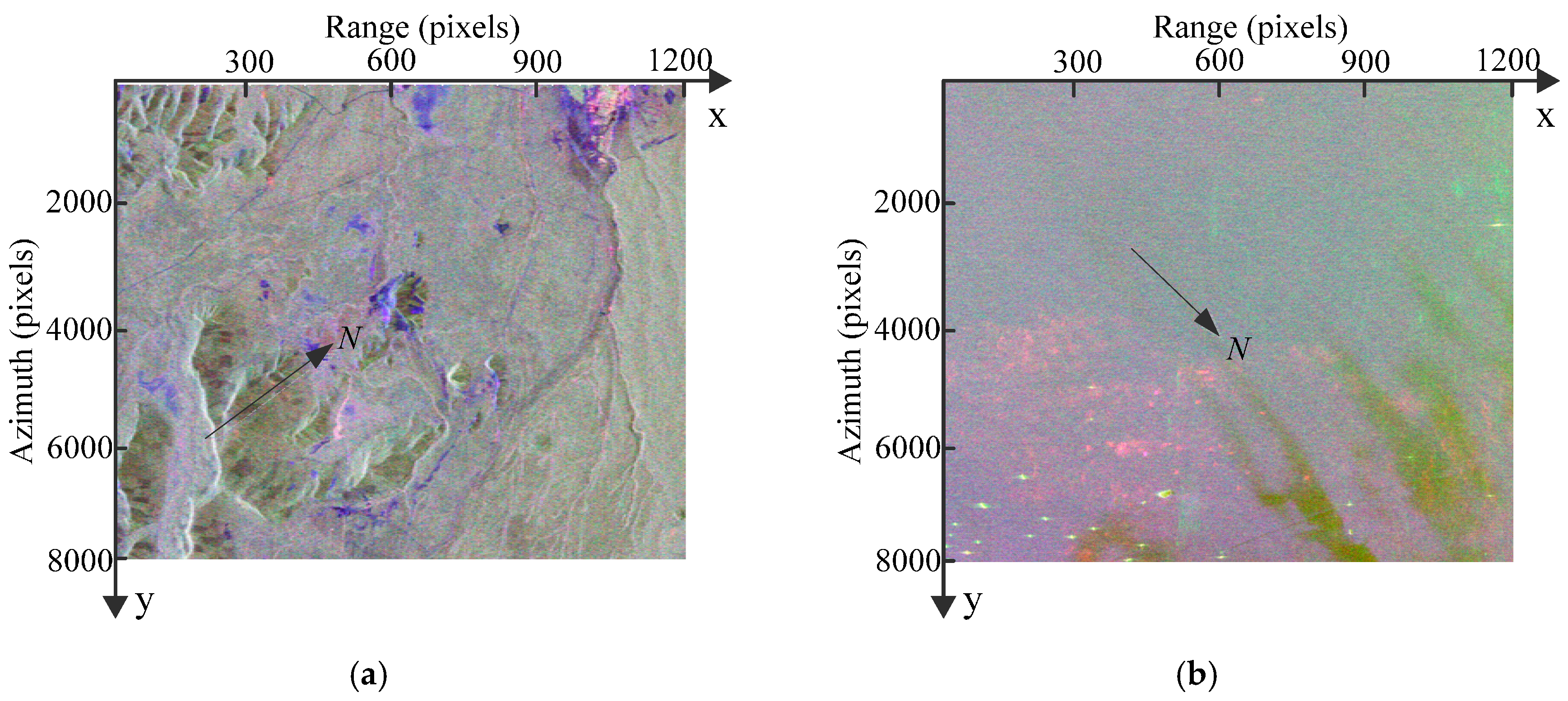
In order to analyze the effects of system errors (system noise, channel phase/amplitude imbalance, and crosstalk) on the proposed CIT individually, the semi-physical simulations using synthetic data of calibrated PALSAR full-pol data, IRI and IGRF models are required. In numerical simulations, two calibrated PALSAR full-pol data sets with different scattering types are used, namely, one from an area near Changbai Mountain (42.17°N, 128.0°E) acquired on 3 December 2007 and one from a seaside area of Qingdao (35.83°N, 120.75°E) acquired on 29 March 2011. Figure 3 shows the corresponding Pauli false-color images [31], and both data sets are composed of pixels in range (x-axis) and azimuth directions (y-axis). N denotes geographical North. The resolutions are about 9.369 m and 3.557 m in range and azimuth directions, respectively.
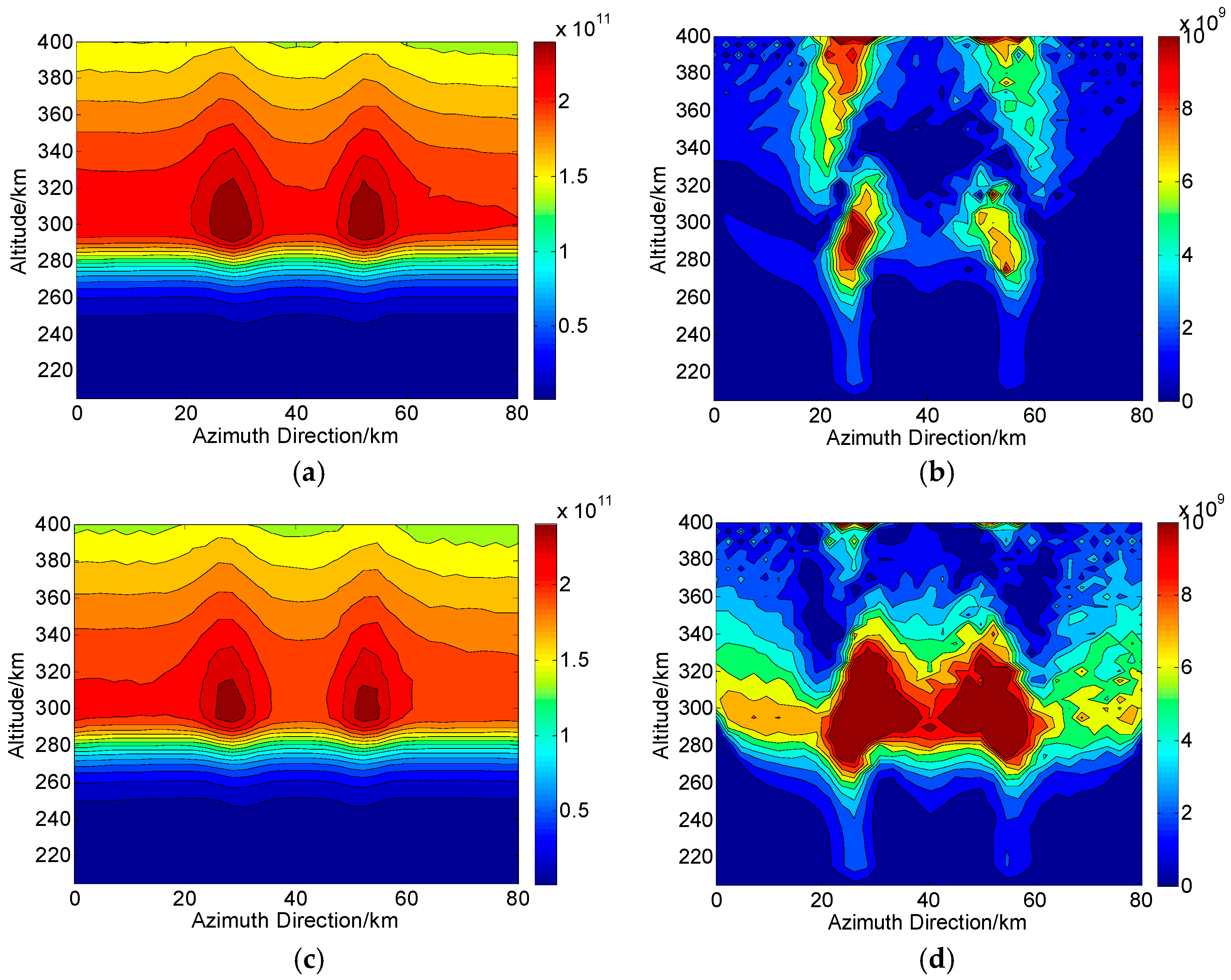
According to the operations in Figure 1, we assume that during one CIT simulation, the whole orbiting length of PolSAR along the azimuth direction is about 120 km and has 75 sampling positions (). The reconstructed area of the ionosphere is set to 80 km long and 204–400 km along azimuth and altitude directions, respectively. Correspondingly, each grid spacing is set to 5 km and 2.5 km along altitude and azimuth directions, respectively. For the distribution of the electron density, two small-scale artificial disturbances are then embedded. This new distribution with ionospheric disturbances is regarded as the “true distribution” to be reconstructed and used for comparison, as shown in Figure 4. On the ground, the imaging scene will be divided into 16 parts along azimuth direction, where each subimage is composed of pixels. Thus, according to the position of azimuth sampling, vectors of ray path and magnetic field, the can be calculated. By combining , and into Equation (10), the true corresponding to each ray path can further be determined. The scattering matrix measured for each ray path is then corrupted by the system errors and .
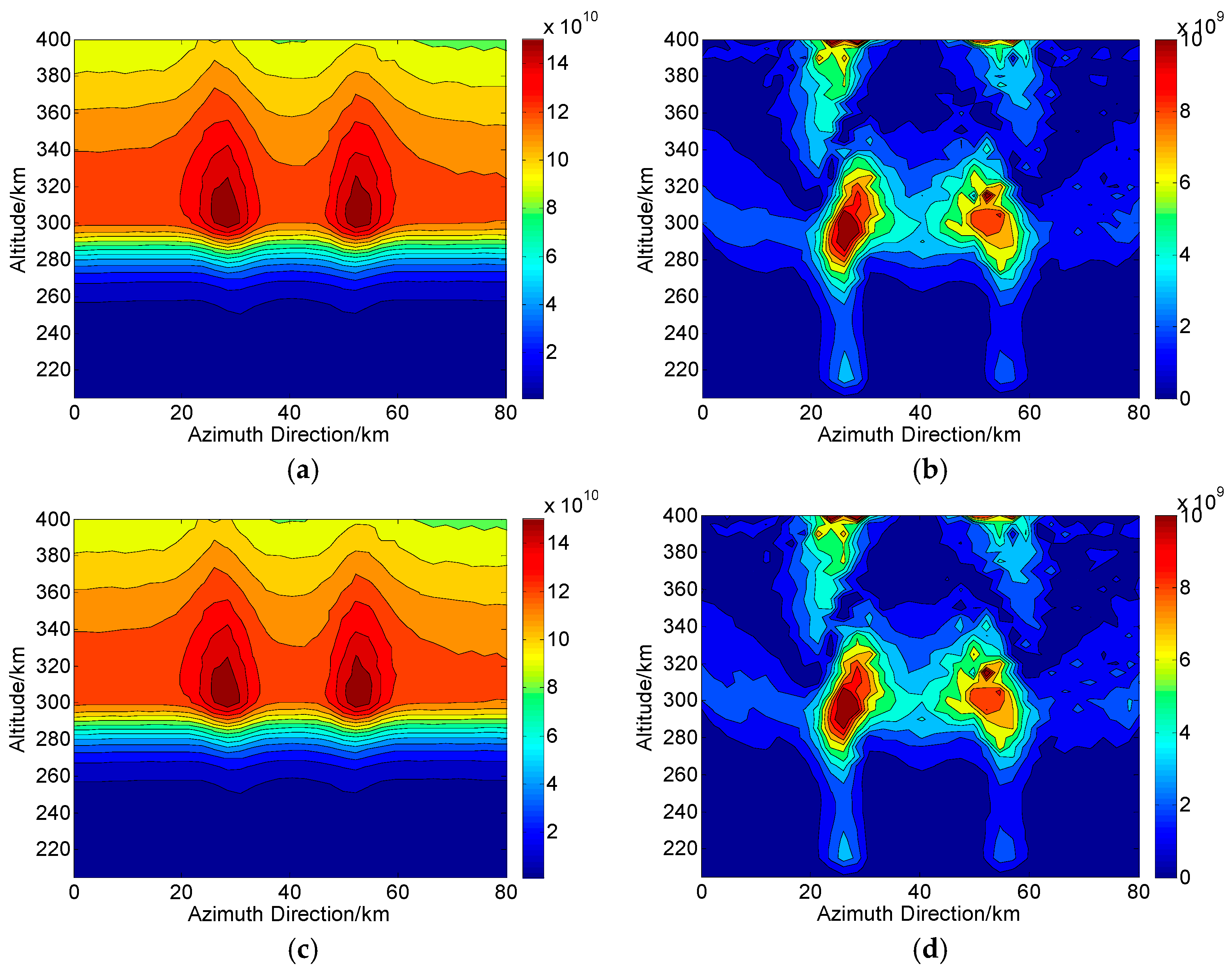
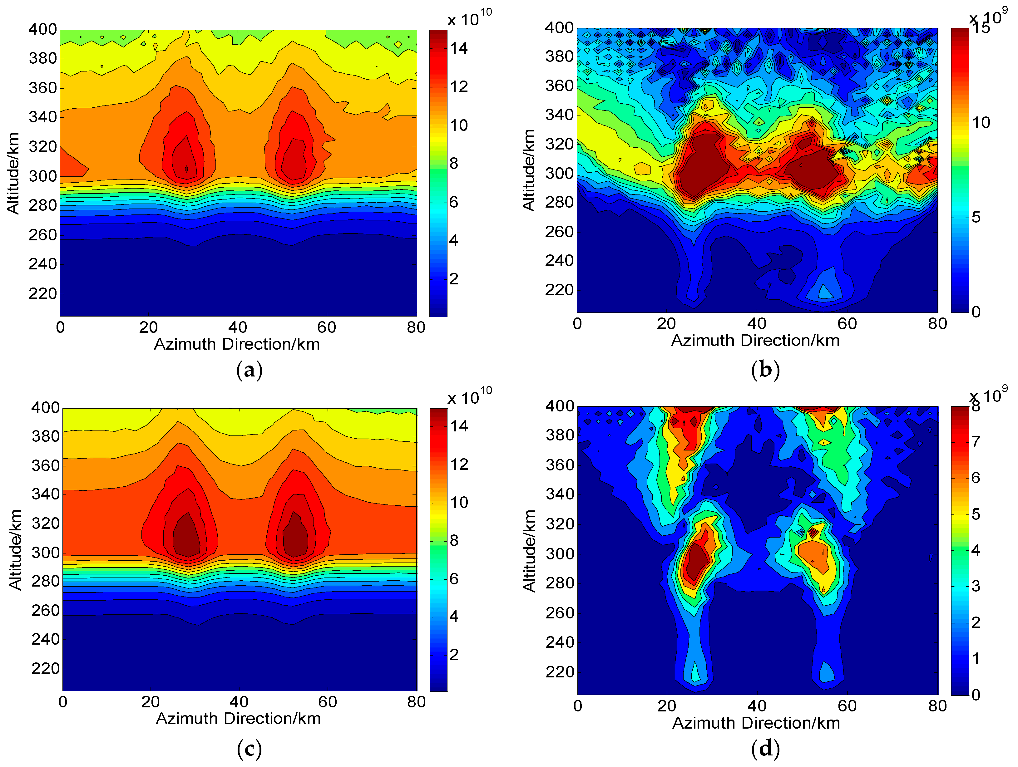
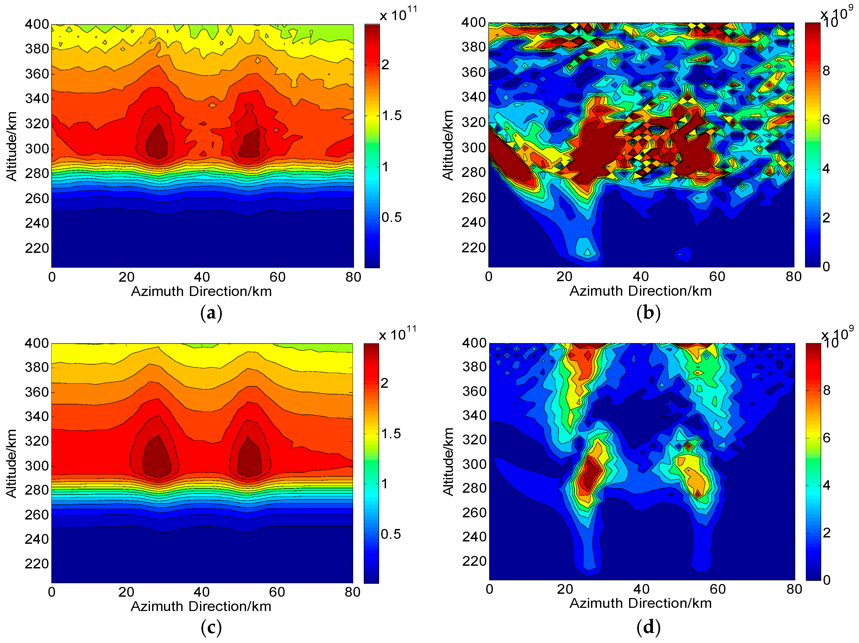
Based on the proposed CIT method without system errors, Figure 5a and Figure 6a show the two-dimensional CIT reconstructions in Changbai and Qingdao, respectively. Figure 5b and Figure 6b show the corresponding two-dimensional absolute deviations between the true (i.e., Figure 4a,b) and reconstructed distributions (i.e., Figure 5a and Figure 6a), and the RMS over the whole images are and , respectively. Similar, Figure 5c and Figure 6c are the two-dimensional CIT reconstructions based on the traditional CIT method [28], where TEC is regarded as the input and first derived from FR when the magnetic field is approximated by a fix value of 300 km. The corresponding absolute deviations are shown in Figure 5d and Figure 6d. The RMS of Figure 5d and Figure 6d are and , respectively. We can see that due to the errors caused by the approximation of magnetic field, obvious errors occur for traditional CIT. Thus, compared with traditional CIT, the proposed CIT method can avoid the approximate error of magnetic field.
4.1. CIT Reconstructions Under the Condition of System Noise
Assume the system noise and FR are the only errors, and the noise power in each channel is the same (i.e., ), the scattering matrix of Equation (2) can be written as (see Appendix A)
According to the process of CIT discussed above, we first evaluate the performances of the FR estimators, as shown in Table 1, Table 2 and Table 3. The RMS error, bias and standard deviation (SD) are defined as
where (, or ) is the retrieved FR value corresponding to each ray path. The units of , and are %. In addition, the signal-to-noise ratio (SNR) can be defined by Chen and Quegan [4]
From Table 1, Table 2 and Table 3, we can see that performs the best in Changbai while is the preferred one in Qingdao. Thus, under the condition of noise, the choice of FR estimators in CIT depends on the scattering type. For , large errors are occurred in both SAR scenes. This is because the mean FR values in areas of Changbai and Qingdao are about 0.8° and 1.45°, respectively, and the Freeman’s estimator is sensitivity to noise near [5].
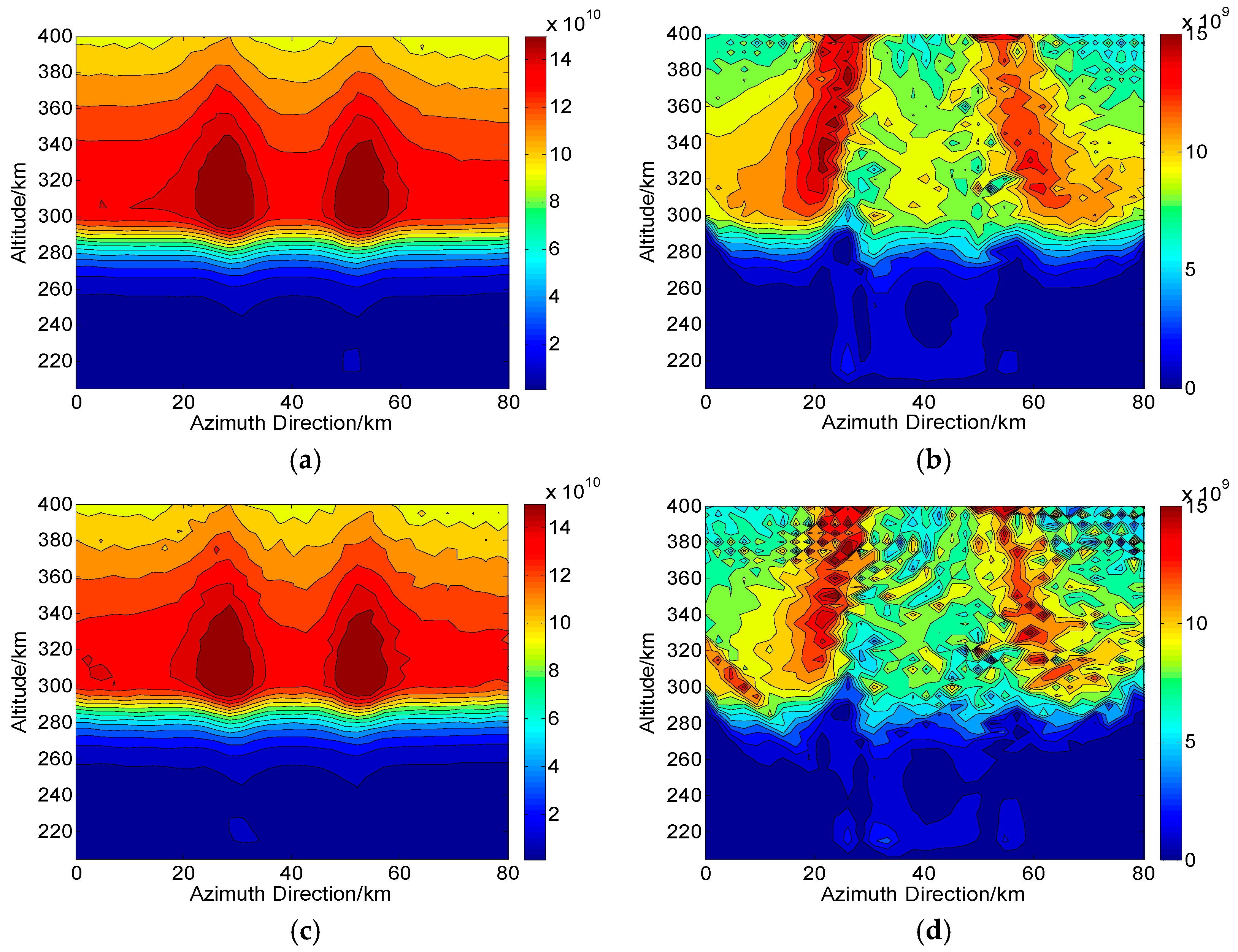
Based on the results of Table 1, Table 2 and Table 3, the final CIT reconstructions in Changbai ( is applied) and Qingdao ( is applied) are shown in Figure 7 and Figure 8, respectively. Figure 7a and Figure 8a are the reconstructed results when . Figure 7b and Figure 8b show the corresponding two-dimensional absolute deviations between the true and reconstructed distributions, and the RMS over the whole images are and , respectively. It can be seen that severe distortions are yielded when SNR is as low as , and the two small-scale disturbances are barely identified. Figure 7c and Figure 8c are the reconstructed results when , a typical condition for radar systems [4], and corresponding absolute deviations are shown in Figure 7d and Figure 8d. We can see that the performance of reconstructions is significantly improved and the two small-scale disturbances are clear. The RMS of Figure 7d and Figure 8d are and , respectively.
4.2. CIT Reconstructions Under the Condition of Channel Imbalance
When the FR and channel phase/amplitude imbalance are considered, the scattering matrix can be written as (see Appendix B)
where the channel imbalances in the receiver and transmitter are assumed to be identical (i.e., ) to simplify the analysis [2,4,32]. The effects of channel phase imbalance, i.e., , on the FR estimators are first evaluated under typical values [2,5]. By using the full-pol data sets of Changbai and Qingdao, the results are shown in Table 4, Table 5 and Table 6. We can see that when the phase imbalance is the dominant error, can perform the smallest RMS error and SD while has the smallest biases. Thus, in order to make a comparison, and are respectively regarded as the input of CIT simulations.
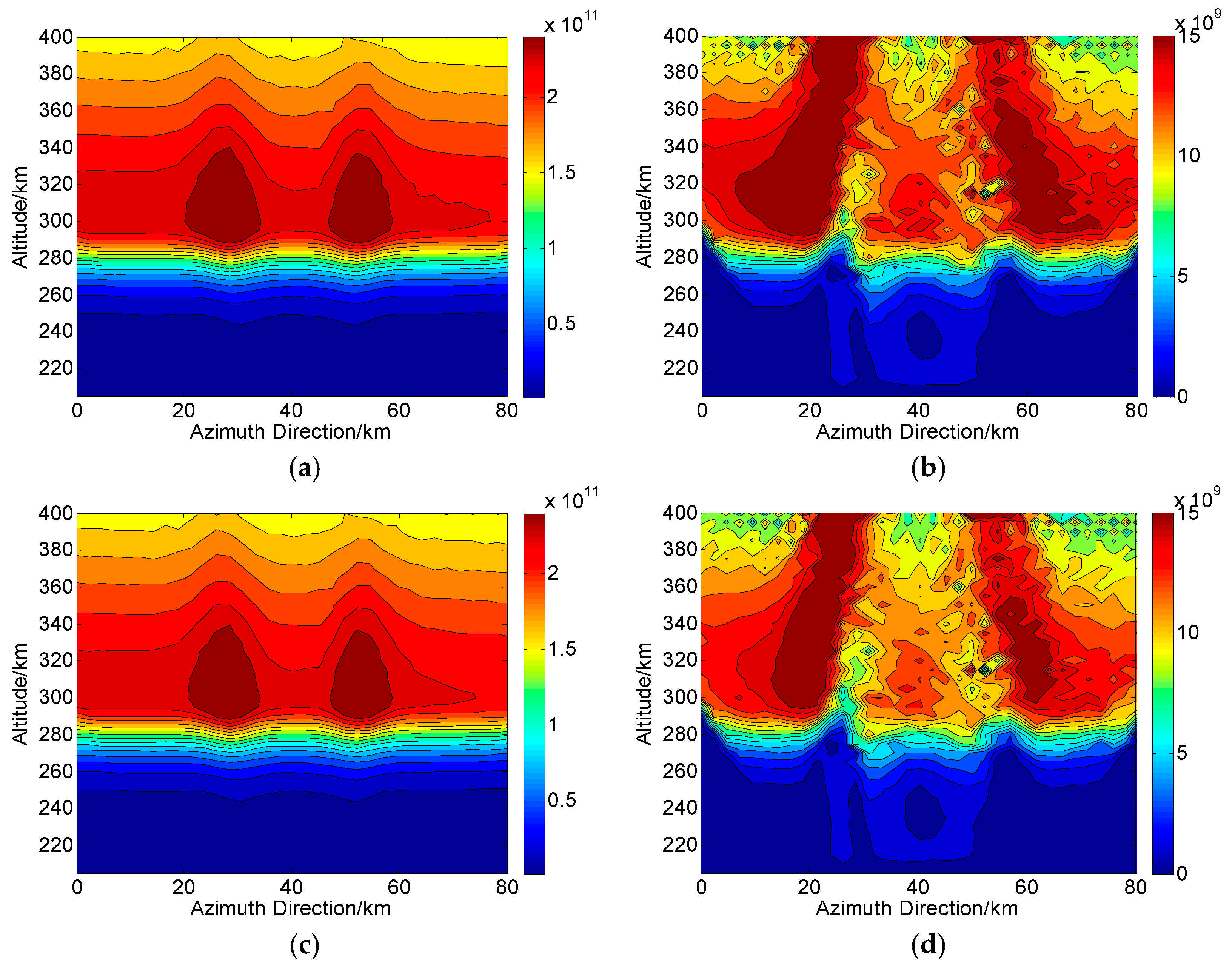
When , Figure 9 and Figure 10 are the final CIT reconstructions in Changbai and Qingdao, respectively. In Changbai, the RMS of corresponding absolute deviations based on and (i.e., Figure 9b,d are and , respectively. Similar, the RMS based on and in Qingdao (i.e., Figure 10b,d) are and , respectively. We can see that both two FR estimators can maintain good performance and the two disturbances are clearly visible. However, the CIT errors become obvious when the phase imbalance is as large as 20°, as shown in Figure 11 and Figure 12. Here, the RMS based on and in Changbai (i.e., Figure 11b,d) are and , respectively. Similar, the RMS in Figure 12b,d are and , respectively. Thus, it can be see that for all conditions, the results based on are better than that based on , especially for large phase imbalance.
Similarly, the effects of amplitude imbalance on the performances of FR estimators are shown in Table 7, Table 8 and Table 9, where the magnitude is less than . We can see that under the conditions of amplitude imbalance, is the preferred estimator in CIT reconstructions. In addition, the statistical characters of are almost unchanged both in Changbai and Qingdao. This is because according to Equation (6) and Equation (15), becomes (see Appendix C)
thus, only depends on .
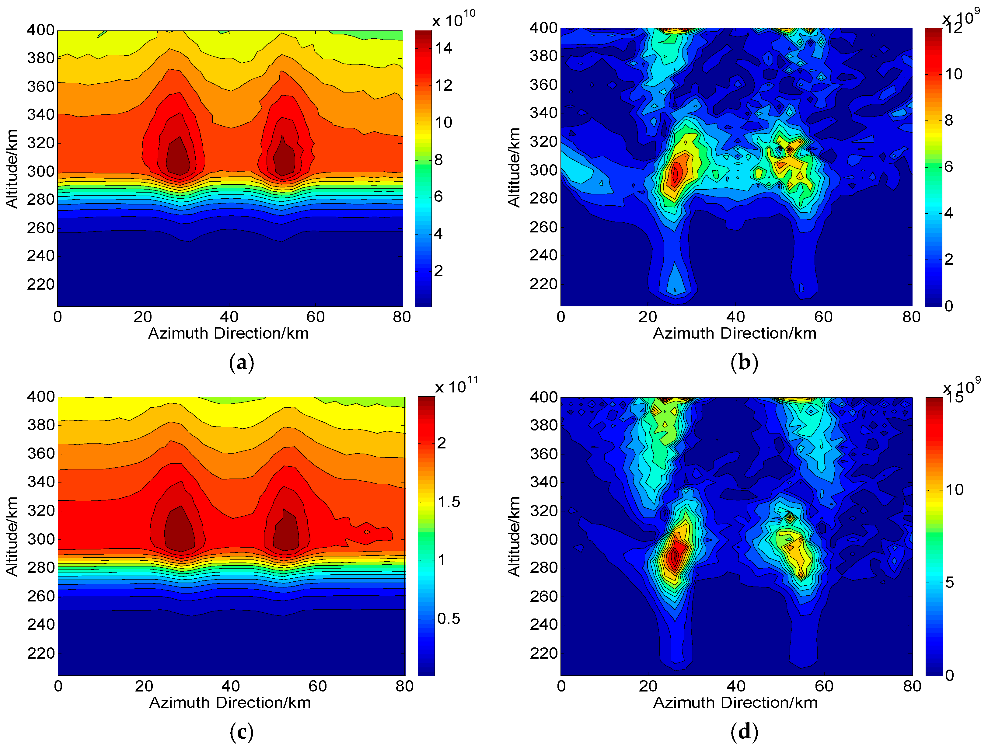
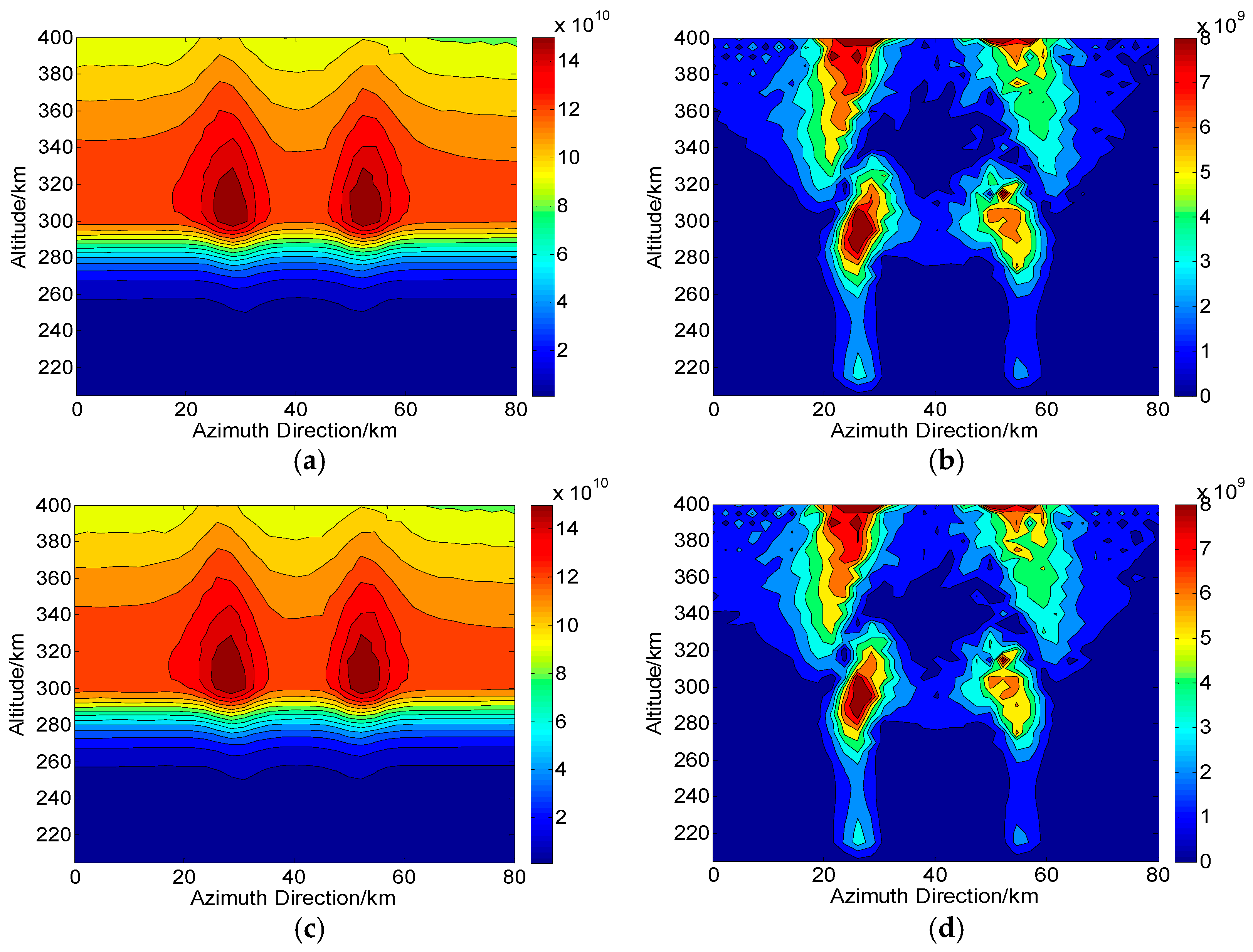
Figure 13 and Figure 14 show the final reconstructions in Changbai and Qingdao, respectively. In simulations of Figure 13a and Figure 14a, the is set to . The RMS of corresponding absolute deviations in Figure 13b and Figure 14b are and , respectively. For Figure 13c and Figure 14c, the is set to and the RMS in Figure 13d and Figure 14d are and , respectively. From the results, we can see that the CIT reconstructions still performs well even if the is as high as . Thus, it can be concluded that compared with noise and phase imbalance, amplitude imbalance is not a problem for CIT reconstruction.
4.3. CIT Reconstructions Under the Condition of Crosstalk
The last system error that should be considered is the crosstalk. Assuming for convenience [2,4,32], the scattering matrix of Equation (2) can be written as (see Appendix D)
Table 10, Table 11 and Table 12 show the performances of FR estimators under the typical values of crosstalk ranging from −15 dB to −35 dB [2,5]. We can see that in area of Changbai, performs the best and can be applied in CIT reconstructions. However, by using the full-pol data of Qingdao, the error of is smaller than that of when the crosstalk is higher than −20 dB. Thus, if the crosstalk is the domain error, the choice of FR estimator in CIT depends on the scattering type and magnitude of crosstalk. The should be applied in our CIT simulations of Qingdao when the crosstalk is equal to and , otherwise is the preferred estimator.
When the crosstalk is set to , Figure 15a and Figure 16a show the CIT reconstructions in Changbai and Qingdao, respectively. The RMS of corresponding absolute deviations in Figure 15b and Figure 16b are and , respectively. It can be seen that the small-scale distributions are difficult to be recognized in both areas when the crosstalk is as high as , an extreme value. It should be noted that from the evaluations in Table 4, the RMS error rapidly decreases with the decrease of crosstalk, which further improves the accurate of CIT reconstructions. Thus, the effect of crosstalk on the CIT is not serious in most conditions. Figure 15c and Figure 16c show the CIT reconstructions when the crosstalk is set to . We can see that significant improvements are demonstrated to clearly show the small-scale distributions. The deviations in Figure 15d and Figure 16d are and , respectively.
4.4. CIT Reconstructions Under the Combination of System Errors
For a realistic situations of the PALSAR system, these calibration errors will appear together. Thus, in order to make a practical value for our CIT technique, the system errors (i.e., noise, channel imbalance and crosstalk) are all considered in this subsection. According to the calibration accuracy of the PALSAR system [32], in simulations, we assume , channel phase imbalance is 2°, channel amplitude imbalance is , and crosstalk is . Table 13 shows the performances of FR estimators under the condition of joint errors, we can see that for the area of Changbai, will be the preferred estimator while performs the best for the area of Qingdao.
Figure 17a,c shows the CIT reconstructions in Changbai ( is used) and Qingdao ( is used), respectively. We can see that when the all system errors are considered, the true ionospehric distribution can still be accurately reconstructed based on the proposed CIT technique, and the two small-scale disturbances are clearly visible. The RMS of corresponding absolute deviations shown in Figure 17b,d are and , respectively. Thus, we can see that after calibration of the PALSAR systems, the proposed CIT technique can give an accurate ionospheric reconstruction in consideration of the residual errors.
5. Conclusions
The distribution of ionospheric electron density is an important part of solar-terrestrial space environment, which can demonstrate the solar and earth activities (magnetic storms, plasma bubbles, midlatitude troughs, ionospheric anomalies caused by earthquakes [8,15], etc.). Monitoring the ionospheric behaviors, especially small-scale ionospheric anomaly, based on the CIT technique is therefore beneficial to these studies. In order to obtain the electron density distribution with high resolution, a modified CIT technique based on the spaceborne PolSAR data is proposed in this paper, where the FR, rather than TEC, is regarded as the input. From the results in Section 4, small-scale distributions can be reconstructed by this proposed CIT technique due to the high spatial resolution of spaceborne SAR, which is inaccessible by conventionally used data source. However, the accuracy of FR retrieval will affect the final CIT reconstructions. The evaluations of three typical FR estimators considering different system errors and scattering types were made. Some conclusions are as follow:
- (1)
- The effect of system noise on FR retrieval depends on both the scattering types and SNR. According to the evaluations, and are the optimal estimators of CIT in areas of Changbai and Qingdao, respectively. The performances of CIT in both areas are improved with the increase of SNR. The small-scale distributions are visible in reconstructions when , a typical configuration for the PALSAR sensors.
- (2)
- For considering the effects of channel phase imbalance, can give the smallest error both in areas of Changbai and Qingdao. From the simulation results, it can be seen that the CIT errors are sensitive to phase imbalance. For amplitude imbalance, should be applied. However, in contrast to phase imbalance and noise, the effects of amplitude imbalance on CIT is small.
- (3)
- The choice of FR estimator considering the crosstalk depends on both scattering types and magnitude of the crosstalk. When the crosstalk is as high as , serious CIT reconstructions are shown. However, with the decrease of the crosstalk, the error of FR retrieval is sharply decreased. The effects of crosstalk on the CIT are limited when the crosstalk is equal to .
In general, the main system effects on CIT are the noise and channel phase imbalance while channel amplitude imbalance and crosstalk can be ignored for most cases. According to the calibration accuracy of the PALSAR system, we evaluate the reconstructions when all the system errors are considered. Accurate results can still be obtained by the proposed CIT technique. It should be noted that we have analyzed other full-pol SAR scenes, and the same results are obtained. In addition, there are other factors that can affect the CIT reconstructions. For example, the lack of horizontal ray paths and the choice of initial distribution in iteration also degrade the accuracy of CIT [14,15]. Combining of the PolSAR and occultation or ground-based ionosonde data can reduce these problems and will be done in our future work.
Acknowledgments
This work was supported by the National Natural Science Foundation of China (NSFC) under Grants 41604157, 41601483 and 61401022, and by the National Key Laboratory of Electromagnetic Environment.
Author Contributions
Cheng Wang, Liang Chen, Haisheng Zhao, Mingming Bian and Zheng Lu initiated the research. Under supervision of Running Zhang, Jian Feng, and Cheng Wang performed the analysis and wrote the manuscript. Liang Chen, Haisheng Zhao and Mingming Bian revised the manuscript. All authors read and approved the final version of the manuscript.
Conflicts of Interest
The authors declare no conflict of interest.
Appendix A
When the system noise and FR are the only errors, the scattering matrix of Equation (2) can be written as
Thus, each factor of M matrix can be written as
Appendix B
Similarly, if the FR and channel phase/amplitude imbalance are considered, and the channel imbalances in the receiver and transmitter are assumed to be identical (i.e., ), the scattering matrix of Equation (2) can be written as
Thus, each factor of M matrix is derived as
Appendix C
When we only consider the amplitude imbalance () in (A4), each factor of (Equations (6) and (7)) is
Then,
Appendix D
If the crosstalk is considered and is assumed, the scattering matrix of Equation (2) becomes
Thus, each factor of the M matrix is
References
- Lawrence, R.S.; Little, C.G.; Chivers, H.A. A survey of ionospheric effects upon earth-space radio propagation. Proc. IEEE 1964, 52, 4–27. [Google Scholar] [CrossRef]
- Freeman, A. Calibration of linearly polarized polarimetric SAR data subject to Faraday rotation. IEEE Trans. Geosci. Remote Sens. 2004, 42, 1617–1624. [Google Scholar] [CrossRef]
- Bickel, S.H.; Bates, R.H.T. Effects of magneto-ionic propagation on the polarization scattering matrix. Proc. IEEE 1964, 53, 1089–1091. [Google Scholar] [CrossRef]
- Chen, J.; Quegan, S. Improved estimators of Faraday rotation in spaceborne polarimetric SAR data. IEEE Geosci. Remote Sens. Lett. 2010, 7, 846–850. [Google Scholar] [CrossRef]
- Rogers, N.C.; Quegan, S. The accuracy of Faraday rotation estimation in satellite synthetic aperture radar images. IEEE Trans. Geosci. Remote Sens. 2014, 52, 4799–4807. [Google Scholar] [CrossRef]
- Meyer, F.; Bamler, R.; Jakowski, N.; Fritz, T. The potential of low-frequency SAR systems for mapping ionospheric TEC distributions. IEEE Geosci. Remote Sens. Lett. 2006, 3, 560–564. [Google Scholar] [CrossRef]
- Jehle, M.; Ruegg, M.; Zuberbuhler, L.; Small, D.; Meier, E. Measurement of ionospheric faraday rotation in simulated and real spaceborne SAR Data. IEEE Trans. Geosci. Remote Sens. 2009, 47, 1512–1523. [Google Scholar] [CrossRef] [Green Version]
- Pi, X.Q.; Freeman, A.; Chapman, B.; Rosen, P.; Li, Z.H. Imaging ionospheric inhomogeneities using spaceborne synthetic aperture radar. J. Geophys. Res. 2011, 116, 1451–1453. [Google Scholar] [CrossRef]
- Pi, X.Q. Ionospheric effects on spacebrone synthetic aperture radar and a new capability of imaging the ionosphere from space. Space Weather 2015, 13, 737–741. [Google Scholar] [CrossRef]
- Kim, J.S.; Papathanassiou, K.P.; Scheiber, R.; Quegan, S. Correcting Distortion of Polarimetric SAR Data Induced by Ionospheric Scintillation. IEEE Trans. Geosci. Remote Sens. 2015, 53, 6319–6335. [Google Scholar]
- Wang, C.; Liu, L.; Chen, L.; Feng, J.; Zhao, H.S. Improved TEC retrieval based on spaceborne PolSAR data. Radio Sci. 2017, 52, 288–304. [Google Scholar] [CrossRef]
- Yizengaw, E.; Dyson, P.L.; Essex, E.A. Ionosphere dynamics over the southern hemisphere during the 31 March 2001 severe magnetic storm using multi-instrument measurement data. Ann. Geophys. 2005, 23, 707–721. [Google Scholar] [CrossRef]
- Wen, D.B.; Yuan, Y.B.; Ou, J.K.; Zhang, K.F. Ionospheric response to the geomagnetic storm on August 21, 2003 over China using GNSS-Based tomographic technique. IEEE Trans. Geosci. Remote Sens. 2010, 48, 3212–3217. [Google Scholar]
- Zhao, H.S.; Xu, Z.W.; Wu, J.; Quegan, S. Ionospheric tomography of small-scale disturbances with a triband beacon: A numerical study. Radio Sci. 2010, 45. [Google Scholar] [CrossRef]
- Zhao, H.S.; Xu, Z.W.; Wu, J.; Wang, Z.G. Ionospheric tomography by combining vertical and oblique ionograms with TEC retrieved from a tri-band beacon. J. Geophys. Res. 2010, 115, 788–802. [Google Scholar] [CrossRef]
- Austen, J.R.; Franke, S.J.; Liu, C.H. Ionospheric imaging using computerized tomography. Radio Sci. 1988, 23, 299–307. [Google Scholar] [CrossRef]
- Pryse, S.E. Radio tomography: A new experimental technique. Surv. Geophys. 2003, 24, 1–38. [Google Scholar] [CrossRef]
- Li, L.L.; Li, F. Ionosphere tomography based on spaceborne SAR. Adv. Space Res. 2008, 42, 1187–1193. [Google Scholar] [CrossRef]
- Wang, C.; Zhang, M.; Xu, Z.W.; Zhao, H.S. TEC retrieval from spacebrone SAR data and its applications. J. Geophys. Res. 2014, 119, 8648–8659. [Google Scholar] [CrossRef]
- Hu, C.; Tian, Y.; Dong, X.; Wang, R.; Long, T. Computerized ionospheric tomography based on geosynchronous SAR. J. Geophys. Res. 2017, 122, 2686–2705. [Google Scholar] [CrossRef]
- Hu, C.; Li, Y.; Dong, X.; Cui, C.; Long, T. Impacts of temporal-spatial variant background ionosphere on repeat-track GEO D-InSAR system. Remote Sens. 2016, 8, 916. [Google Scholar] [CrossRef]
- Jehle, M.; Frey, O.; Small, D.; Meier, E. Measurement of ionospheric TEC in spaceborne SAR data. IEEE Geosci. Remote Sens. Lett. 2010, 48, 2460–2468. [Google Scholar] [CrossRef]
- Lizuka, K.; Tateishi, R. Estimation of CO2 sequestration by the forests in Japan discriminating precise tree age category using remote sensing techniques. Remote Sens. 2015, 7, 15082–15113. [Google Scholar]
- Xiong, S.; Peter, J.; Li, G. The application of ALOS/PALSAR InSAR to measure subsurface penetration depths in deserts. Remote Sens. 2017, 9, 638. [Google Scholar] [CrossRef]
- Meyer, F. Performance Requirements for Ionospheric Correction of Low-Frequency SAR Data. IEEE Trans. Geosci. Remote Sens. 2011, 49, 3694–3702. [Google Scholar] [CrossRef]
- Yuel, S.H. Estimates of Faraday rotation with passive microwave polarimetry for microwave remote sensing of Earth surfaces. IEEE Trans. Geosci. Remote Sens. 2000, 38, 2434–2438. [Google Scholar]
- Cushley, A.C.; Noel, J.M. Ionospheric tomography using ADS-B signals. Radio Sci. 2014, 49, 549–563. [Google Scholar] [CrossRef]
- Wang, C.; Chen, L.; Liu, L.; Yang, J.; Lu, Z.; Feng, J.; Zhao, H.S. Robust computerized ionospheric tomography based on spaceborne polarimetric SAR data. IEEE J. Sel. Top. Appl. Earth Obs. Remote Sens. 2017, 10, 4022–4031. [Google Scholar] [CrossRef]
- Budden, K.G. Radio Waves in the Ionosphere: The Mathematical Theory of the Reflection of Radio Waves from Stratified Ionized Layers; Cambridge University Press: Cambridge, UK, 1961. [Google Scholar]
- Bust, G.S.; Mitchell, C.N. History, current state, and future directions of ionospheric imaging. Rev. Geophys. 2008, 46, 394–426. [Google Scholar] [CrossRef]
- Lee, J.S.; Pottier, E. Polarimetric Radar Imaging: From Basics to Applications; CRC Press: Florida, FL, USA, 2009. [Google Scholar]
- Meyer, F.; Nicoll, J.B. Prediction, detection, and correction of Faraday rotation in full-polarimetic L-band SAR data. IEEE Trans. Geosci. Remote Sens. 2008, 46, 3076–3086. [Google Scholar] [CrossRef]
Figure 1.
Map of two-dimensional CIT using FR angles.
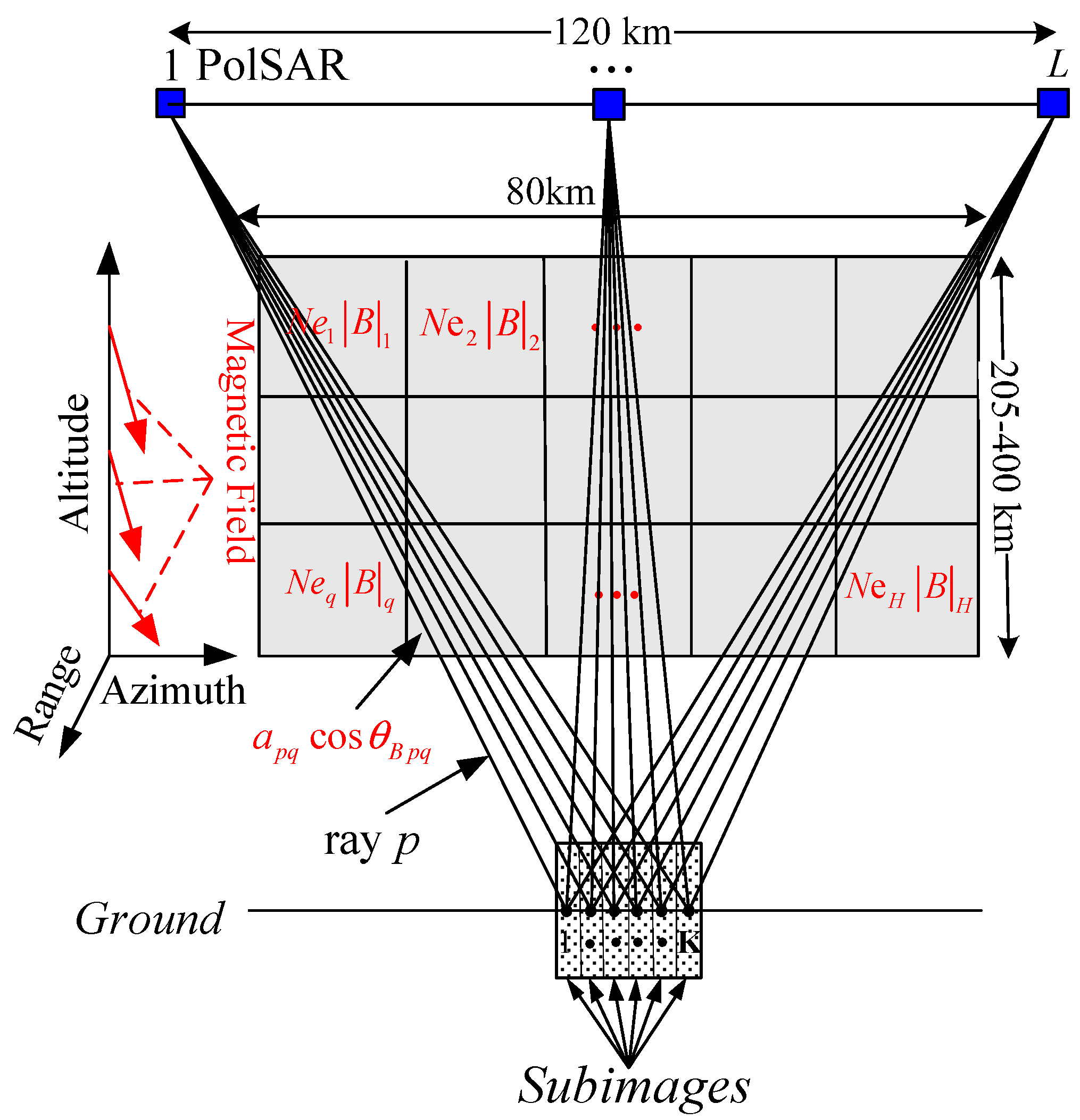
Figure 2.
The flowchart of the proposed CIT technique.

Figure 3.
The PALSAR polarimetric images in two areas. (a) Changbai Mountain (N, E) acquired on 3 December 2007 and (b) Qingdao (N, E) acquired on 29 March 2011.
Figure 3.
The PALSAR polarimetric images in two areas. (a) Changbai Mountain (N, E) acquired on 3 December 2007 and (b) Qingdao (N, E) acquired on 29 March 2011.

Figure 4.
The true distributions of electron density in areas of (a) Changbai and (b) Qingdao. The unit of the electron density is .
Figure 4.
The true distributions of electron density in areas of (a) Changbai and (b) Qingdao. The unit of the electron density is .
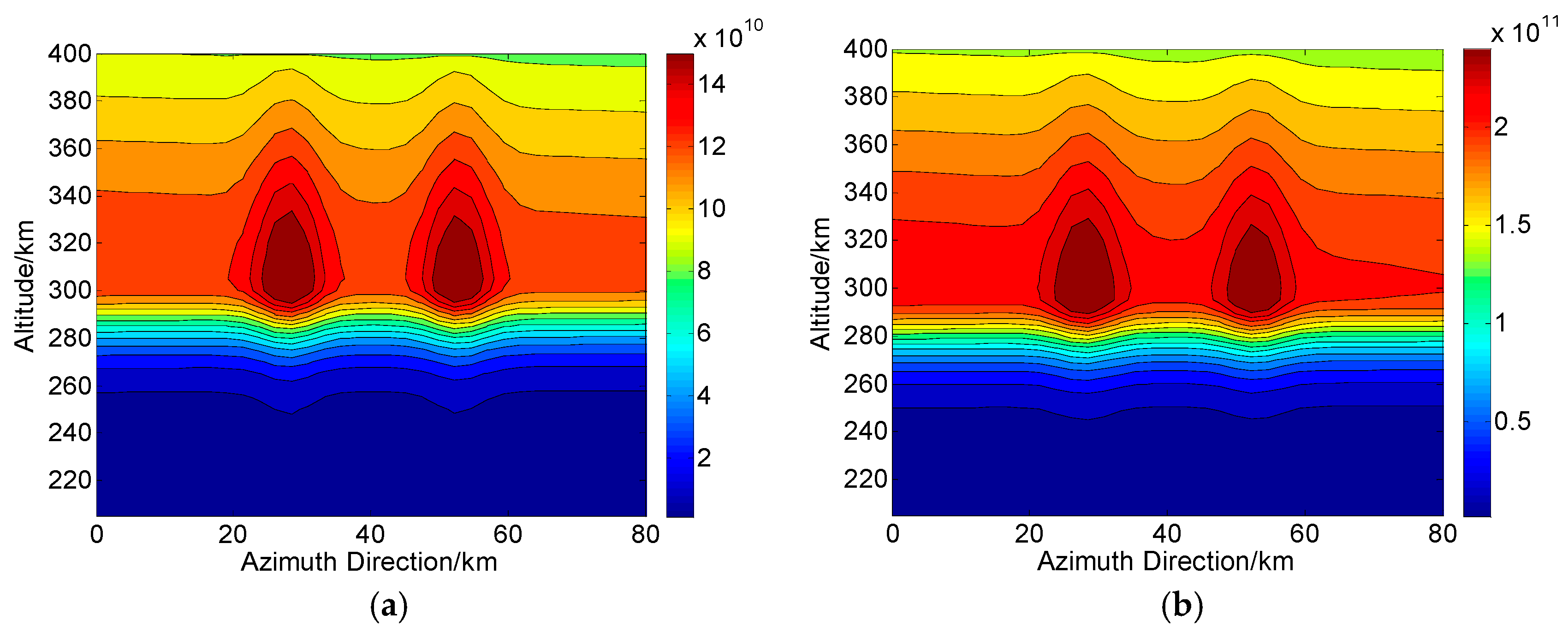
Figure 5.
Two-dimensional CIT reconstructions without system errors in Changbai. (a,c) are the reconstructed results based on proposed and traditional CIT methods, respectively. (b,d) are the corresponding absolute deviations between the true and reconstructed results. The unit of the electron density is .
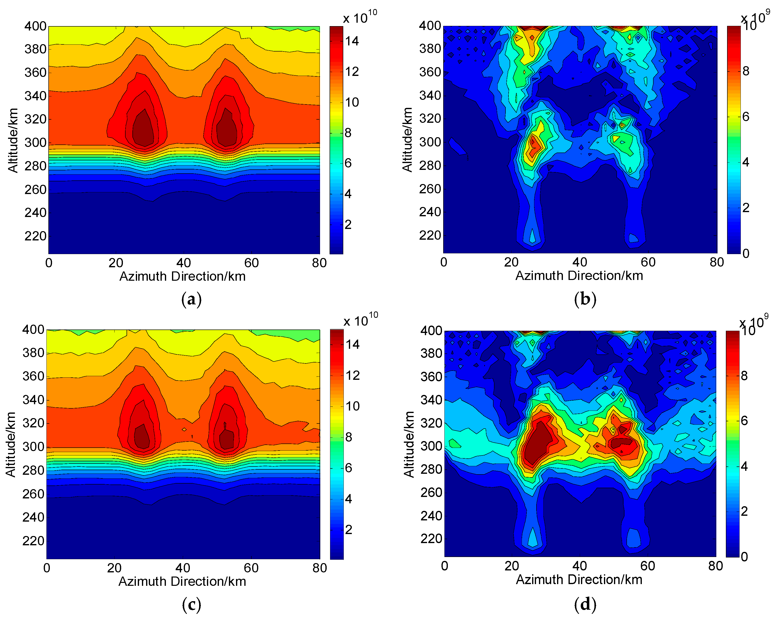
Figure 6.
Two-dimensional CIT reconstructions without system errors in Qingdao. (a,c) are the reconstructed results based on proposed and traditional CIT methods, respectively. (b,d) are the corresponding absolute deviations between the true and reconstructed results. The unit of the electron density is .

Figure 7.
Two-dimensional CIT reconstructions under the condition of system noise in Changbai ( is used). (a,c) are the reconstructed results with and , respectively. (b,d) are the corresponding absolute deviations between the true and reconstructed results. The unit of the electron density is .
Figure 7.
Two-dimensional CIT reconstructions under the condition of system noise in Changbai ( is used). (a,c) are the reconstructed results with and , respectively. (b,d) are the corresponding absolute deviations between the true and reconstructed results. The unit of the electron density is .
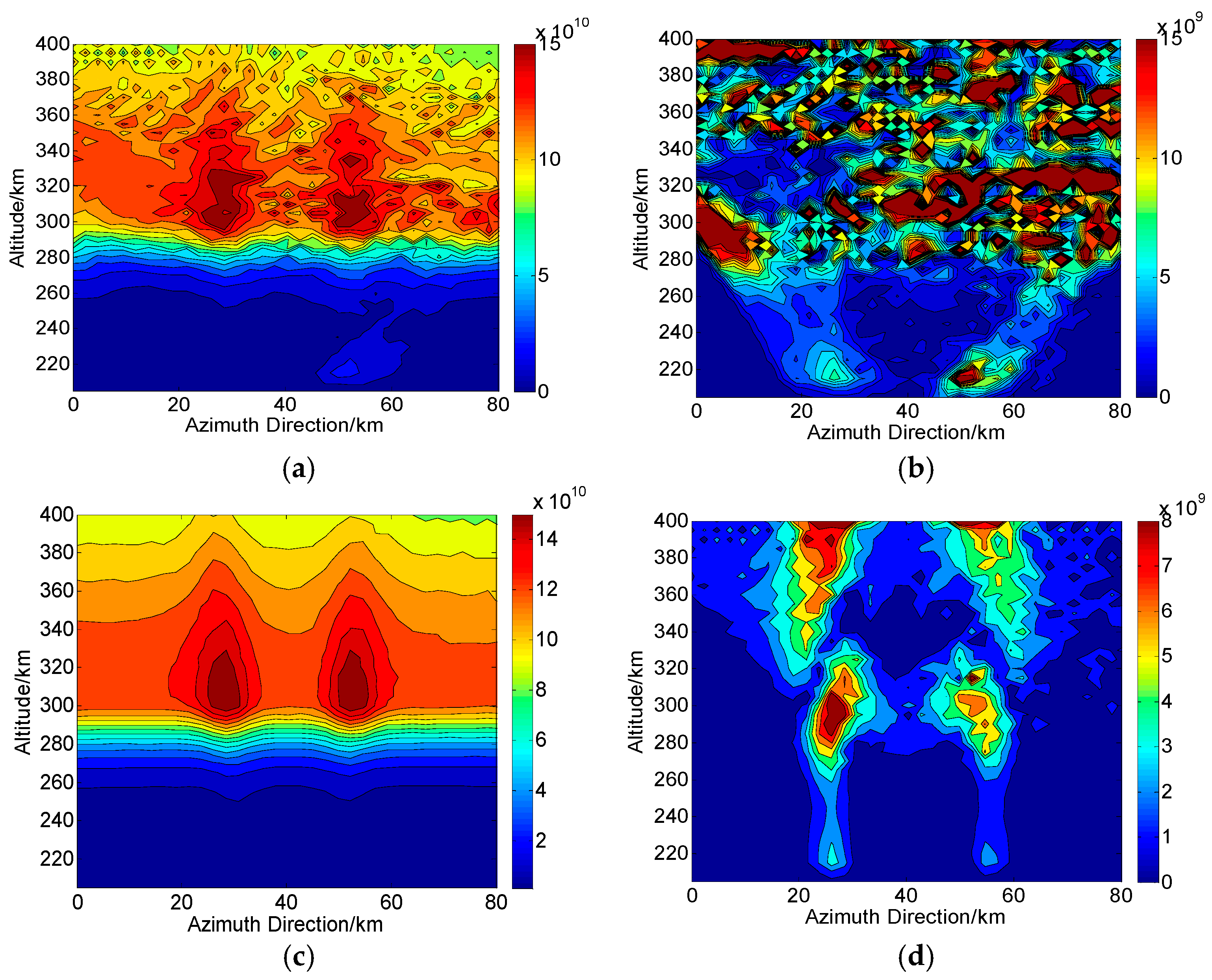
Figure 8.
Two-dimensional CIT reconstructions under the condition of system noise in Qingdao ( is used). (a,c) are the reconstructed results with and , respectively. (b,d) are the corresponding absolute deviations between the true and reconstructed results. The unit of the electron density is .
Figure 8.
Two-dimensional CIT reconstructions under the condition of system noise in Qingdao ( is used). (a,c) are the reconstructed results with and , respectively. (b,d) are the corresponding absolute deviations between the true and reconstructed results. The unit of the electron density is .
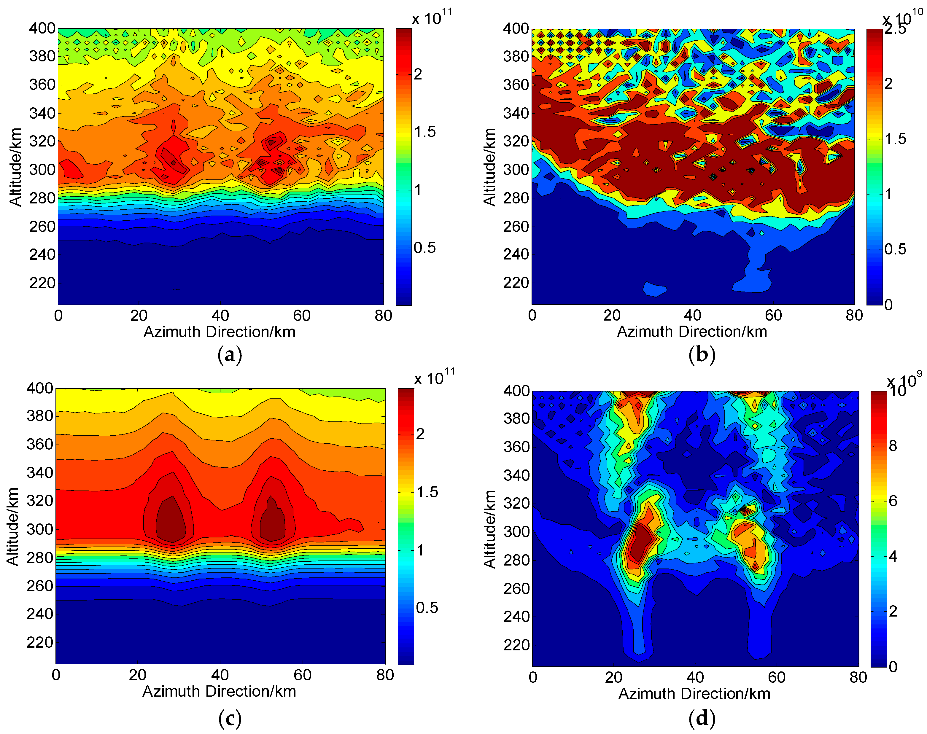
Figure 9.
Two-dimensional CIT reconstructions under the condition of channel phase imbalance () in Changbai. (a,c) are the reconstructed results based on and , respectively. (b,d) are the corresponding absolute deviations between the true and reconstructed results. The unit of the electron density is .

Figure 10.
Two-dimensional CIT reconstructions under the condition of channel phase imbalance () in Qingdao. (a,c) are the reconstructed results based on and , respectively. (b,d) are the corresponding absolute deviations between the true and reconstructed results. The unit of the electron density is .
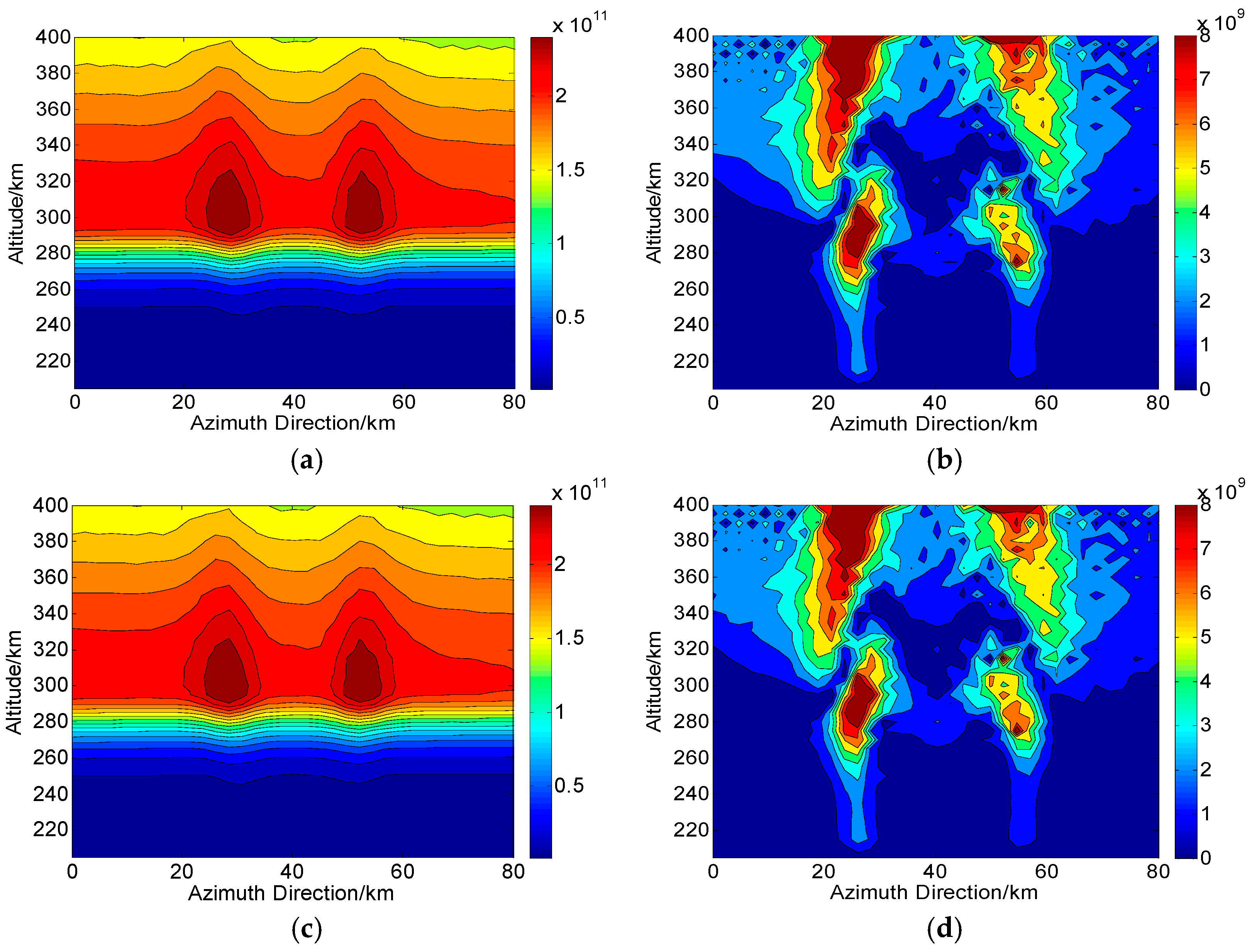
Figure 11.
Two-dimensional CIT reconstructions under the condition of channel phase imbalance () in Changbai. (a,c) are the reconstructed results based on and , respectively. (b,d) are the corresponding absolute deviations between the true and reconstructed results. The unit of the electron density is .

Figure 12.
Two-dimensional CIT reconstructions under the condition of channel phase imbalance () in Qingdao. (a,c) are the reconstructed results based on and , respectively. (b,d) are the corresponding absolute deviations between the true and reconstructed results. The unit of the electron density is .

Figure 13.
Two-dimensional CIT reconstructions under the condition of channel amplitude imbalance in Changbai ( is used). (a,c) are the reconstructed results with and , respectively. (b,d) are the corresponding absolute deviations between the true and reconstructed results. The unit of the electron density is .

Figure 14.
Two-dimensional CIT reconstructions under the condition of channel amplitude imbalance in Qingdao ( is used). (a,c) are the reconstructed results with and , respectively. (b,d) are the corresponding absolute deviations between the true and reconstructed results. The unit of the electron density is .

Figure 15.
Two-dimensional CIT reconstructions under the condition of crosstalk in Changbai ( is used). (a,c) are the reconstructed results with and , respectively. (b,d) are the corresponding absolute deviations between the true and reconstructed results. The unit of the electron density is .
Figure 15.
Two-dimensional CIT reconstructions under the condition of crosstalk in Changbai ( is used). (a,c) are the reconstructed results with and , respectively. (b,d) are the corresponding absolute deviations between the true and reconstructed results. The unit of the electron density is .

Figure 16.
Two-dimensional CIT reconstructions under the condition of crosstalk in Qingdao. (a) ( is used) and (c) ( is used) are the reconstructed results with and , respectively. (b,d) are the corresponding absolute deviations between the true and reconstructed results. The unit of the electron density is .

Figure 17.
Two-dimensional CIT reconstructions under the condition of joint errors. (a) ( is used) and (c) ( is used) are the reconstructed results in areas of Changbai and Qingdao, respectively. (b,d) are the corresponding absolute deviations between the true and reconstructed results. The unit of the electron density is .

Table 1.
RMS error () under the condition of system noise.
| SNR (dB) | RMS Error (%) | |||||
|---|---|---|---|---|---|---|
| Changbai | Qingdao | |||||
| 5 | 19.1023 | 866.7750 | 3.1956 | 10.6599 | 457.1695 | 14.1860 |
| 10 | 9.2369 | 475.1484 | 1.4204 | 4.0307 | 237.6931 | 7.8032 |
| 15 | 3.4335 | 239.2308 | 0.8279 | 1.3728 | 109.9127 | 4.0608 |
| 20 | 1.5564 | 109.0368 | 0.3182 | 0.5284 | 44.7311 | 1.9436 |
| 25 | 0.9041 | 44.1177 | 0.2153 | 0.2032 | 16.1787 | 1.4127 |
| 30 | 0.3327 | 15.9300 | 0.0991 | 0.1384 | 5.4124 | 0.5717 |
Table 2.
Bias () under the condition of system noise.
| SNR (dB) | Bias (%) | |||||
|---|---|---|---|---|---|---|
| Changbai | Qingdao | |||||
| 5 | 18.6803 | −858.3574 | 1.1071 | 7.8405 | −452.2203 | 7.8584 |
| 10 | 8.0336 | −469.8182 | −0.9973 | 3.2375 | −234.7492 | 3.3109 |
| 15 | 3.1830 | −235.7411 | 0.2154 | 1.2264 | −108.1120 | 1.3629 |
| 20 | 1.1940 | −107.1453 | −0.1585 | 0.5594 | −43.7774 | 0.6791 |
| 25 | 0.3286 | −43.1128 | −0.0424 | 0.0342 | −15.7346 | 0.2223 |
| 30 | 0.1523 | −15.4490 | 0.0385 | −0.0017 | −5.2271 | 0.0380 |
Table 3.
SD () under the condition of system noise.
| SNR (dB) | SD (%) | |||||
|---|---|---|---|---|---|---|
| Changbai | Qingdao | |||||
| 5 | 8.0833 | 121.1693 | 2.9652 | 1.2226 | 65.3801 | 17.1186 |
| 10 | 5.3539 | 70.6254 | 1.5441 | 0.8802 | 37.3999 | 7.5438 |
| 15 | 2.1559 | 39.2181 | 0.7358 | 0.4353 | 19.7724 | 4.6861 |
| 20 | 1.0907 | 20.4720 | 0.3469 | 0.2412 | 9.2965 | 1.7415 |
| 25 | 0.5715 | 9.5487 | 0.1984 | 0.1454 | 3.7366 | 1.1294 |
| 30 | 0.2959 | 3.8175 | 0.1311 | 0.1013 | 1.3163 | 0.5045 |
Table 4.
RMS error () under the condition of channel phase imbalance.
| Channel Phase Imbalance (°) | RMS Error (%) | |||||
|---|---|---|---|---|---|---|
| Changbai | Qingdao | |||||
| 5 | 1.5075 | 1.5863 | 5.0152 | 0.4340 | 0.4644 | 5.7890 |
| 10 | 3.6991 | 3.9594 | 9.2409 | 1.5537 | 1.6645 | 7.4793 |
| 15 | 6.6352 | 7.2038 | 13.9008 | 3.3994 | 3.6423 | 9.8274 |
| 20 | 10.4286 | 11.4409 | 19.5022 | 6.0230 | 6.4697 | 13.0879 |
Table 5.
Bias () under the condition of channel phase imbalance.
| Channel Phase Imbalance (°) | Bias (%) | |||||
|---|---|---|---|---|---|---|
| Changbai | Qingdao | |||||
| 5 | −1.4987 | −1.5859 | −4.8996 | −0.4337 | −0.4643 | −5.7350 |
| 10 | −3.6691 | −3.9582 | −9.0977 | −1.5528 | −1.6643 | −7.4330 |
| 15 | −6.6716 | −7.2012 | −13.7565 | −3.3974 | −3.6420 | −9.7901 |
| 20 | −10.3174 | −11.4362 | −19.3646 | −6.0199 | −6.4692 | −13.0582 |
Table 6.
SD () under the condition of channel phase imbalance.
| Channel Phase Imbalance (°) | SD (%) | |||||
|---|---|---|---|---|---|---|
| Changbai | Qingdao | |||||
| 5 | 0.1620 | 0.0371 | 1.0709 | 0.0180 | 0.0096 | 0.7895 |
| 10 | 0.4708 | 0.0983 | 1.6208 | 0.0523 | 0.0251 | 0.8311 |
| 15 | 0.9164 | 0.1910 | 1.9986 | 0.1175 | 0.0482 | 0.8558 |
| 20 | 1.5199 | 0.3261 | 2.3139 | 0.1954 | 0.0809 | 0.8814 |
Table 7.
RMS error () under the condition of channel amplitude imbalance.
| Channel Amplitude Imbalance (dB) | RMS Error (%) | |||||
|---|---|---|---|---|---|---|
| Changbai | Qingdao | |||||
| 0.1 | 0.1525 | 0.2570 | 0.0066 | 0.0688 | 0.0659 | 0.0066 |
| 0.2 | 0.2958 | 0.5045 | 0.0266 | 0.1233 | 0.1187 | 0.0266 |
| 0.3 | 0.4270 | 0.7358 | 0.0594 | 0.1632 | 0.1570 | 0.0594 |
| 0.4 | 0.5509 | 0.9570 | 0.1060 | 0.1890 | 0.1820 | 0.1060 |
| 0.5 | 0.6630 | 1.1639 | 0.1654 | 0.1982 | 0.1933 | 0.1652 |
Table 8.
Bias () under the condition of channel amplitude imbalance.
| Channel Amplitude Imbalance (dB) | Bias (%) | |||||
|---|---|---|---|---|---|---|
| Changbai | Qingdao | |||||
| 0.1 | −0.1198 | −0.2539 | −0.0066 | −0.0684 | −0.0655 | −0.0066 |
| 0.2 | −0.2281 | −0.4980 | −0.0266 | −0.1225 | −0.1178 | −0.0266 |
| 0.3 | −0.3215 | −0.7257 | −0.0594 | −0.1617 | −0.1555 | −0.0594 |
| 0.4 | −0.4041 | −0.9430 | −0.1060 | −0.1868 | −0.1796 | −0.1058 |
| 0.5 | −0.4738 | −1.1459 | −0.1654 | −0.1949 | 0.1897 | −0.1652 |
Table 9.
SD () under the condition of channel amplitude imbalance.
| Channel Amplitude Imbalance (dB) | SD (%) | |||||
|---|---|---|---|---|---|---|
| Changbai | Qingdao | |||||
| 0.1 | 0.0945 | 0.0401 | 0.00001 | 0.0072 | 0.0074 | 0.00001 |
| 0.2 | 0.1884 | 0.0811 | 0.00001 | 0.0142 | 0.0149 | 0.00001 |
| 0.3 | 0.2811 | 0.1216 | 0.00002 | 0.0222 | 0.0222 | 0.00002 |
| 0.4 | 0.3745 | 0.1629 | 0.00002 | 0.0281 | 0.0296 | 0.00003 |
| 0.5 | 0.4639 | 0.2042 | 0.00002 | 0.0356 | 0.0370 | 0.00005 |
Table 10.
RMS error () under the condition of crosstalk.
| Crosstalk (dB) | RMS Error (%) | |||||
|---|---|---|---|---|---|---|
| Changbai | Qingdao | |||||
| −15 | 8.8421 | 7.6382 | 7.7358 | 6.2014 | 6.0407 | 2.5106 |
| −20 | 3.7897 | 2.8994 | 2.9776 | 1.9464 | 1.8950 | 1.1415 |
| −25 | 1.7467 | 1.1683 | 1.2207 | 0.5906 | 0.5700 | 0.9784 |
| −30 | 0.8633 | 0.5115 | 0.5437 | 0.1698 | 0.1623 | 0.6808 |
| −35 | 0.4496 | 0.2430 | 0.2621 | 0.0437 | 0.0413 | 0.4264 |
Table 11.
Bias () under the condition of crosstalk.
| Crosstalk (dB) | Bias (%) | |||||
|---|---|---|---|---|---|---|
| Changbai | Qingdao | |||||
| −15 | 8.6232 | 7.5837 | 7.6724 | 5.4012 | 5.4406 | −1.8124 |
| −20 | 3.5849 | 2.8467 | 2.9162 | 1.6463 | 1.6949 | −1.5488 |
| −25 | 1.5885 | 1.1245 | 1.1700 | 0.5925 | 0.5669 | −0.8016 |
| −30 | 0.7551 | 0.4788 | 0.5064 | 0.1684 | 0.1612 | −0.6044 |
| −35 | 0.3811 | 0.2207 | 0.2369 | 0.0426 | 0.0416 | −0.3885 |
Table 12.
SD () under the condition of crosstalk.
| Crosstalk (dB) | SD (%) | |||||
|---|---|---|---|---|---|---|
| Changbai | Qingdao | |||||
| −15 | 1.9561 | 0.9114 | 0.9888 | 1.1464 | 1.1382 | 1.0981 |
| −20 | 1.2295 | 0.5506 | 0.6017 | 0.8232 | 0.8218 | 0.7813 |
| −25 | 0.7268 | 0.3172 | 0.3481 | 0.1390 | 0.1224 | 0.5612 |
| −30 | 0.4186 | 0.1800 | 0.1980 | 0.0832 | 0.0681 | 0.3135 |
| −35 | 0.2387 | 0.1017 | 0.1120 | 0.0393 | 0.0385 | 0.1757 |
Table 13.
The performances of FR estimators under the condition of joint errors.
| Performances | Changbai | Qingdao | ||||
|---|---|---|---|---|---|---|
| RMS error (%) | 3.6572 | 262.1338 | 1.8965 | 1.4348 | 120.5995 | 6.6420 |
| Bias (%) | 3.5491 | −258.7012 | −1.7362 | 1.3959 | −118.7056 | −5.5683 |
| SD (%) | 2.9604 | 42.3003 | 0.8634 | 0.5181 | 21.2925 | 4.9092 |
© 2017 by the authors. Licensee MDPI, Basel, Switzerland. This article is an open access article distributed under the terms and conditions of the Creative Commons Attribution (CC BY) license (http://creativecommons.org/licenses/by/4.0/).
Share and Cite
MDPI and ACS Style
Wang, C.; Chen, L.; Zhao, H.; Lu, Z.; Bian, M.; Zhang, R.; Feng, J. Ionospheric Reconstructions Using Faraday Rotation in Spaceborne Polarimetric SAR Data. Remote Sens. 2017, 9, 1169. https://doi.org/10.3390/rs9111169
AMA Style
Wang C, Chen L, Zhao H, Lu Z, Bian M, Zhang R, Feng J. Ionospheric Reconstructions Using Faraday Rotation in Spaceborne Polarimetric SAR Data. Remote Sensing. 2017; 9(11):1169. https://doi.org/10.3390/rs9111169
Chicago/Turabian StyleWang, Cheng, Liang Chen, Haisheng Zhao, Zheng Lu, Mingming Bian, Running Zhang, and Jian Feng. 2017. "Ionospheric Reconstructions Using Faraday Rotation in Spaceborne Polarimetric SAR Data" Remote Sensing 9, no. 11: 1169. https://doi.org/10.3390/rs9111169
Note that from the first issue of 2016, this journal uses article numbers instead of page numbers. See further details here.