
Mapping Radar Glacier Zones and Dry Snow Line in the Antarctic Peninsula Using Sentinel-1 Images

1
Chinese Antarctic Center of Surveying and Mapping, Wuhan University, Wuhan 430079, China
2
Key Laboratory of Polar Surveying and Mapping, National Administration of Surveying, Mapping and Geoinformation, Wuhan 430079, China
*
Author to whom correspondence should be addressed.
Remote Sens. 2017, 9(11), 1171; https://doi.org/10.3390/rs9111171
Submission received: 28 August 2017
/
Revised: 2 November 2017
/
Accepted: 10 November 2017
/
Published: 15 November 2017
(This article belongs to the Special Issue Snow Remote Sensing)
Abstract
:Surface snowmelt causes changes in mass and energy balance, and endangers the stabilities of the ice shelves in the Antarctic Peninsula (AP). The dynamic changes of the snow and ice conditions in the AP were observed by Sentinel-1 images with a spatial resolution of 40 m in this study. Snowmelt detected by the special sensor microwave/imager (SSM/I) is used to study the relationship between summer snowmelt and winter synthetic aperture radar (SAR) backscatter. Radar glacier zones (RGZs) classifications were conducted based on their differences in liquid snow content, snow grain size, and the relative elevations. We developed a practical method based on the simulations of a microwave scattering model to classify RGZs by using Sentinel-1 images in the AP. The summer snowmelt detected by SSM/I and Sentinel-1 data are compared between 2014 and 2015. The SSM/I-derived melting days is used to validate the winter dry snow line (DSL). RGZs derived from Sentinel-1 images suggest that snowmelt expanded from inland of the Larsen C Ice Shelf to the coastal area, whereas an opposite direction was found in the George VI Ice Shelf. The long melting season in the grounding zone of the Larsen C Ice Shelf may result from the adiabatically-dried föhn winds on the east side of the AP. As the uppermost limit of summer snowmelt, DSL was mapped based on the winter Sentinel-1 mosaic of the AP. Compared with the SSM/I-derived melting days, the winter DSL mainly distributed in the areas melted for one to three days in summer. DSL elevations on the Palmer Land increased from south to north.
1. Introduction
The seasonal and interannual changes of freeze–thaw cycles on ice sheets result in the formations of different glacier facies. Wet snow absorbs significantly more incident solar radiation than dry snow because of the much lower albedo. The increased solar radiation absorption leads to a positive feedback to produce more snowmelt [1]. Therefore, snowmelt plays an important role in the mass and energy balance of the polar regions. The temporal and spatial distribution of snowmelt leads to the formation of different glacier facies, and the variations in glacier facies represent the changes of climate [2,3]. The Antarctic ice shelf snowmelt is particularly sensitive to climate change [4]. As the northernmost part of the Antarctic continent, warming in the Antarctic Peninsula (AP) was reported more rapidly than in the rest of Antarctica [5].
In situ measurements of snowmelt in the polar regions are limited and difficult. Active and passive microwave remote sensing data have been used to map the spatial distribution of surface snowmelt over the Antarctic continent. Studies based on microwave radiometers, synthetic aperture radar (SAR) and scatterometers used brightness temperature (Tb) and backscattering coefficient (σ0) at different channels to estimate the snowmelt in Antarctica [6,7,8,9]. When a snowpack starts to melt, the emissivity and absorptivity increase significantly because of the abrupt increase of the dielectric constant, leading to the sudden increase of Tb and decrease of σ0 [10,11]. Methods based on thresholding Tb and σ0 time series with a constant or regionally variable were used to detect snowmelt [6,12,13,14,15]. The edges of freeze–thaw cycles can also be identified by using wavelet transform methods [16,17].
Compared with radiometer and scatterometer images, SAR images display higher spatial resolution, which enables us to study the detailed pattern of snowmelt, glacial facies, and snow line. In SAR images, backscatter from snow and ice surface is dependent on snow density, liquid water content, grain size, stratigraphy, and surface roughness [18,19]. Different snow zones on a glacier are identifiable on SAR images [2,20,21,22,23,24]. These radar glacier zones (RGZs), including wet snow, frozen percolation, dry snow, superimposed ice, and bare ice radar zone, can be classified by σ0 and elevations [8,18]. The distribution of RGZs depend on terrain and climate conditions. In the Antarctic, where air temperature is much lower than the temperature of mountain glaciers, snowmelt occurs on the flat ice shelves, and meltwater flow is limited due to the relatively high latitude. As a result, the superimposed ice radar zone is absent [16]. On the other hand, there is no dry snow zone for the places with all the snow and ice surface melting in summer.
The transient firn line is the boundary between the bare ice radar zone and wet snow radar zone (summer) or frozen percolation radar zone (winter), which documents the current uppermost limit of the ablation area. At the end of the ablation season, the transient firn line is often regarded as the equilibrium line, which is a key parameter for the glaciers’ mass balance [19]. In winter, the boundary of frozen percolation radar zone and dry snow radar zone represents the uppermost limit of the last summer snowmelt, and the position is regarded as the dry snow line (DSL) [8]. Various SAR images, including European remote sensing satellite (ERS), Radarsat, Envisat, Advanced Land Observing Satellite (ALOS), has been used in the mapping of wet snow in seasonal snow cover by using σ0, incidence angle, and polarization information [25,26,27,28]. Various methods, such as visual interpretation, supervised classification, and machine learning algorithms, have been used in the classification of RGZs for the icefields at high latitudes and altitudes [22,23,24,29,30]. In the Antarctic and Greenland ice sheet, snowmelt occurs at low latitudes and altitudes frequently. The seasonal monitoring of glacier zones is important in order to understand the impact of meteorological parameters of the stability, energy, and mass balance of the ice sheets. Clustering algorithm and region classification based on backscatter and texture properties have been used in the mapping of RGZs on the ice sheets [16,31].
In the AP, the pattern of surface snowmelt and melt ponds highlighted a potential contributing process to the collapses of ice shelves [32]. The boundaries between glacier zones were found to be climate-related in the AP. As the uppermost limit of summer snowmelt, the elevation of the DSL always indicates significant climate changes in the AP [8]. An upward significant shift of the DSL is believed to be related with the change in the snow cover properties under extreme melting conditions, while a downward shift of the DSL is a consequence of the continuous accumulation of dry and fine-grained snow and the absence of melt event for several years. During the last decade of 20th century, a significant upward shift of the DSL in the AP was interpreted as a response to the increase of high temperature events [33]. DSL elevation in the AP was found to show good correlation with the summer air temperature [34].
Sentinel-1A and Sentinel-1B were launched in 2014 and 2016, respectively, and provide continuous imagery over the polar regions. With the two-satellite constellation, six-day exact repeat pass observations can be used for the monitoring of detailed patterns of snowmelt in the AP. We developed a practical method based on the simulations of a microwave scattering model to classify summer RGZs by using Sentinel-1 images in the AP (Section 3). We compare the summer snowmelt detected by the special sensor microwave/imager (SSM/I) and Sentinel-1. The SSM/I-derived melt area is used to validate the DSL mapped by winter Sentinel-1 mosaic. The mapping of summer RGZs and winter DSL in the AP are shown in Section 4, followed by the discussion and conclusions of this study in Section 5 and Section 6.
2. Study Area and Data Sets
2.1. Study Area
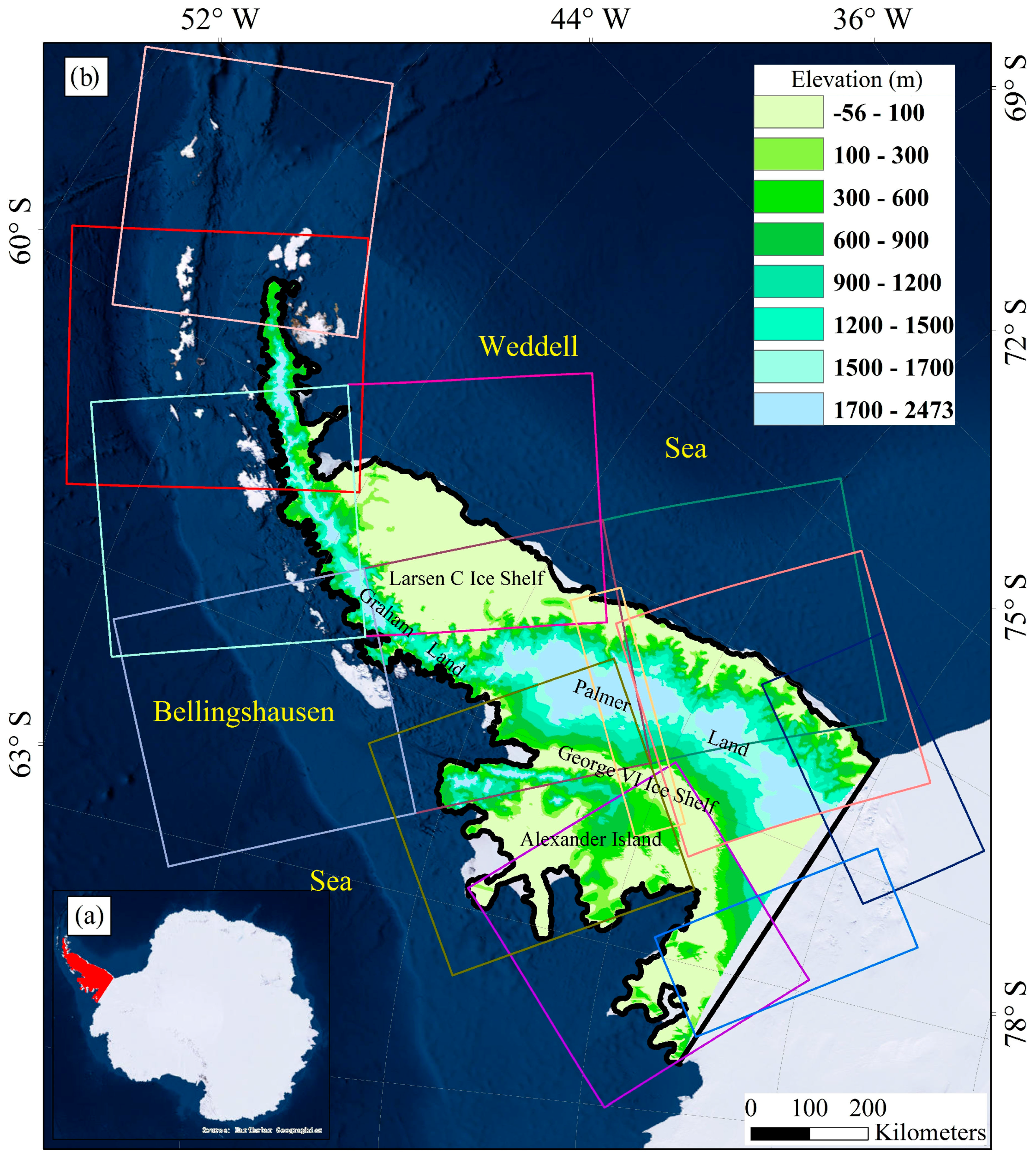
The AP is a northward extension (approximately 1300 km) of Antarctica toward the southern tip of South America (Figure 1). The AP is ice-covered and mountainous, with long melt seasons [35]. Strong rising trends in the melting conditions were found in the records of the meteorological stations in the AP, where warming was more rapid than in the rest of Antarctica [5,36]. Recent studies found that the loss of ice shelf mass in west AP is accelerating [37]. Meltwater percolated into the bottom of the ice will weaken and even disintegrate the ice shelves. Recently, some ice shelves in the AP experienced dramatic break-ups, including the catastrophic collapse of Larsen B in 2002 when the surface snowmelt was three times greater than the average [9,38].
2.2. Data Sets
2.2.1. SSM/I Passive Microwave Data
Carried aboard the Defense Meteorological Satellite Program (DMSP) satellites, SSM/I data were used to detect snowmelt since 1987 [17,39,40,41]. The Level-3 Southern Hemisphere EASE-Grid Brightness Temperature data set provided by the National Snow and Ice Data Center (NSIDC, http://nsidc.org/) was used in this study [42]. The spatial resolution is 25 km for all channels in both ascending and descending orbits. We processed the data spanning from 1 July 2014 to 30 June 2015 in Antarctica. The 19.35 GHz Tb in horizontal polarization was used to derive the daily snowmelt distribution in the AP. Snowmelt detected by the SSM/I is used in three aspects in this study: (1) to study the relationship between summer snowmelt and winter SAR backscatter; (2) to compare with the summer snowmelt detected by Sentinel-1; and (3) to validate the DSL mapped by winter Sentinel-1 mosaic.
2.2.2. Sentinel-1 Images
With the purpose of imaging all global landmasses, oceans, coastal zones, and shipping routes at high resolution, Sentinel-1A and Sentinel-1B were launched in 2014 and 2016, providing timely and easily accessible information in a six-day exact repeat [43]. The two polar-orbiting satellites operating in C-band (5.4 GHz) are able to acquire imagery regardless of the weather. The Sentinel-1 SAR instrument operates in four exclusive imaging modes, namely, the Wave, Strip Map, Extra Wide (EW) Swath, and Interferometric Wide Swath modes, with different resolutions and coverage. Sentinel-1 has single polarization (VV or HH) for the Wave mode, and dual polarization (VV + VH or HH + HV) for other modes [44]. This study used the HH polarized Ground Range Detected (GRD) imagery product in EW mode to derive RGZs and DSL in the AP (see the image frames in Figure 1b). The GRD products were multilooked and projected to ground range using an Earth ellipsoid model. Detailed information of the 22 images obtained from the European Space Agency (ESA) is listed in Table 1.
These horizontally polarized images observed the AP at a spatial resolution of 40 m. The radiometric calibration, terrain correction, Lee filter with a window size of 7 × 7, and the mosaicking of the images were conducted with the ESA’s Sentinel Application Platform. The incidence angles of the EW mode images range from 18° to 46°, resulting in the reduction of backscatter energy from near to far range. The wide range of incidence angles affects the detection and classification of RGZ. A cosine-based normalization method was applied to limit the σ0 variations [45,46]:
where σ0ref means the normalized backscattering coefficient; θ is the local incidence angle; σ0θ is the measured backscatter; and θref is the reference angle, which was set as 30° in this study.
3. Methodology
Due to the lack of in situ observation, RGZs and DSL derived from Sentinel-1 images are compared with SSM/I-derived snowmelt in this study. Snowmelt detected by the SSM/I is used to study the relationship between summer snowmelt and winter SAR backscatter. We also compare the summer snowmelt detected by the SSM/I and Sentinel-1. The SSM/I-derived melt area is used to validate the DSL mapped by winter Sentinel-1 mosaic. In this section, we present the melt detection method for the SSM/I. A practical method to classify RGZs is developed based on the simulations of a microwave scattering model.
3.1. Snowmelt Detection Using SSM/I Data
A thresholding method proposed by Zwally and Fiegles (1994) [6] was used to recognize snowmelt, which was in good agreement with snowmelt derived from air/surface temperature in Antarctica [47]. Snowmelt is identified when horizontally polarized 19.35 GHz Tb exceeds the winter mean plus 30 K, illustrated as follows:
where t is the time, Twm is the winter (from May to July) mean Tb, and m(t) represents snowmelt, with m = 1 indicating melt and m = 0 indicating freeze. Figure 2 shows the horizontally polarized 19.35 GHz Tb of a melting pixel (67.81°S, 64.64°W) on the Larsen C Ice Shelf and a frozen pixel (72.21°S, 63.63°W) on Palmer Land. Melting signals (the red line above 190 K) were clearly observed during summer in the first place, whereas no snowmelt was detected for the other one (the green line).
3.2. RGZ Classification Using Sentinel-1
RGZs show altitudinal zonation on the glaciers. In general, bare ice, wet snow, frozen percolation, and dry snow radar zones distribute successively with the elevations [8]. Melting signals were found within the areas lower than 1700 m by the SSM/I in this study. Arigony-Neto et al. [34] reported that the elevation is higher than 800 in the dry snow radar zone, and lower than 500 m for bare ice in the AP. RGZs can be also characterized by their backscattering characteristics. Dominated by specular reflection, the bare ice radar zone shows minimal change throughout the freeze/thaw cycles. The wet snow radar zone is dark because of the strong absorption and limited penetration of the C-band microwave; scattering occurs only at the wet-snow surface [28,30]. Freezing and thawing repeatedly, the frozen percolation radar zone shows high winter backscatter intensities due to the ice layers and coarse grain in the snowpacks. The wavelength of the C-band microwave is much greater than the snow grain size in dry snow packs, so the backscatter returns in the dry snow radar zone is weak, because of the low dielectric losses and deep penetration [2,48,49,50].
The MEMLS3&a developed by Proksch et al. (2015) [51] was used in this study to simulate the backscatter of RGZs due to the limited observations in the AP. As an extension of the microwave emission model of layered snowpacks (MEMLS), MEMLS3&a applies six-flux theory to describe multiple volume scattering and absorption. The model outputs Tb and σ0 in the snowpacks by inputting the snow density, thickness, salinity, temperatures of interfaces, exponential correlation length, and liquid water content of each layer. Other general model parameters are also needed, including the snow–ground reflectivity, cross-polarization ratio, and mean slope of surface undulation. Simulations were in good agreement with in situ observations [51,52,53].
A set of controlled experiments was conducted using MEMLS3&a. We assume that the snowpacks are homogeneous in the vertical direction, and both the ground and snow temperatures are 273.15 K for slight snowmelt. The incidence angle was set to 30°, and the corresponding sky brightness temperature for the C-band is 8 K [54]. Snow–ice reflectivity at 5.4 GHz was set to 0.15 and 0.6 in horizontal and vertical polarizations, respectively, according to a study on sea ice [55]. The mean slope of snow surface undulation and the cross-polarization ratio were set to 0.1 and 0.15, respectively [51]. The exponential correlation length in MEMLS3&a is used to describe the snow structure, which is a function of snow density and grain size [56,57], and is illustrated as follows:
where Pex is the exponential correlation length, ρsnow and ρice are snow and ice density, respectively, and d represents the snow grain size. Ice density was set as 917 kg/m3 in this study.
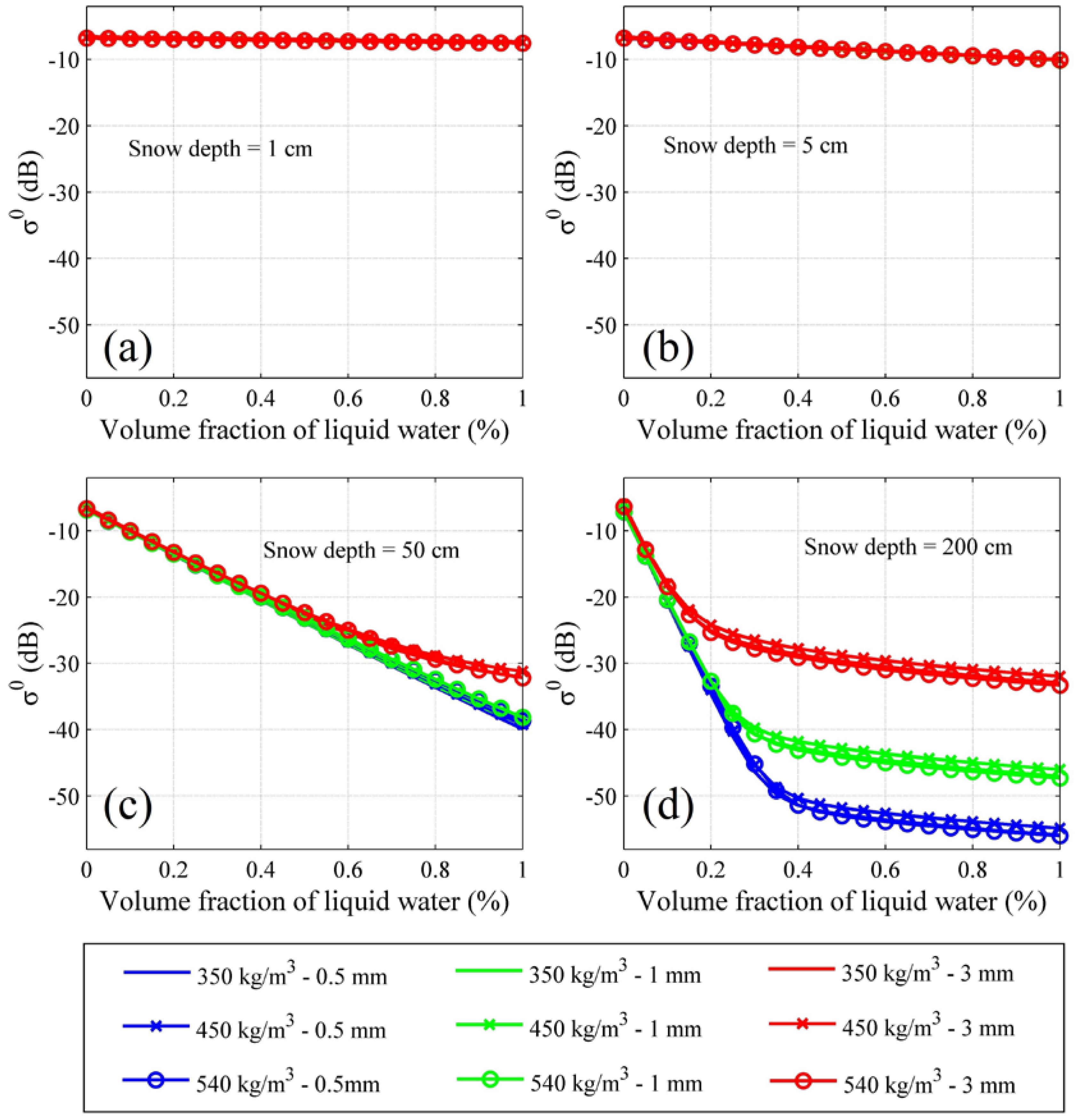
Snow profiles designed in the simulations referenced a study that links the SAR data with snow pit measurements in the AP [19]. We simulated the changes of σ0 in the transitions from dry to wet snow regimes (with snow liquid water from 0 to 1% in volume). With snow density ranging from 350 kg/m3 to 540 kg/m3 and snow grain size ranging from 0.5 mm to 3 mm, different snow profiles were designed in the simulations. As shown in Figure 3a, σ0 changes slightly and maintains less than −6.5 dB when snow depth was set as 1 cm (regarded as bare ice). The results also suggest that even minimal liquid water in shallow snowpacks (e.g., 5 cm) can lead to a sharp decrease in σ0 (Figure 3b). Much larger drops are found in the simulations of thicker snowpacks. Denser snowpacks with small grains are more sensitive to liquid water (Figure 3c,d). The spectral behavior of the wet snow can be dominated by the meltwater when the liquid water content is 1% by volume [58]. For the snowpacks thicker than 5 cm, C-band σ0 decreases by at least 4 dB in every case when liquid water reaches 1% by volume.
Grain size is more than 2 mm in coarse-grained snowpacks and less than 2 mm in fine-grained snowpacks [59], which dominate the backscatter in frozen percolation and dry snow radar zones, respectively. As shown in Figure 4, the C-band σ0 in snowpacks with coarse grain (3–8 mm) and fine grain (0.5–2 mm) increase and decrease with snow depth. The σ0 of the coarse-grained snowpacks rises above −6.5 dB quickly but keeps below −6.5 dB in the fine-grained snowpacks. The simulations suggest that a frozen percolation radar zone experiencing heavy snowmelt in summer turns bright on SAR images in winter, whereas the dry snow radar zone with high accumulation would be dark. The results indicate a clear boundary (i.e., the DSL) between the two zones on SAR images.
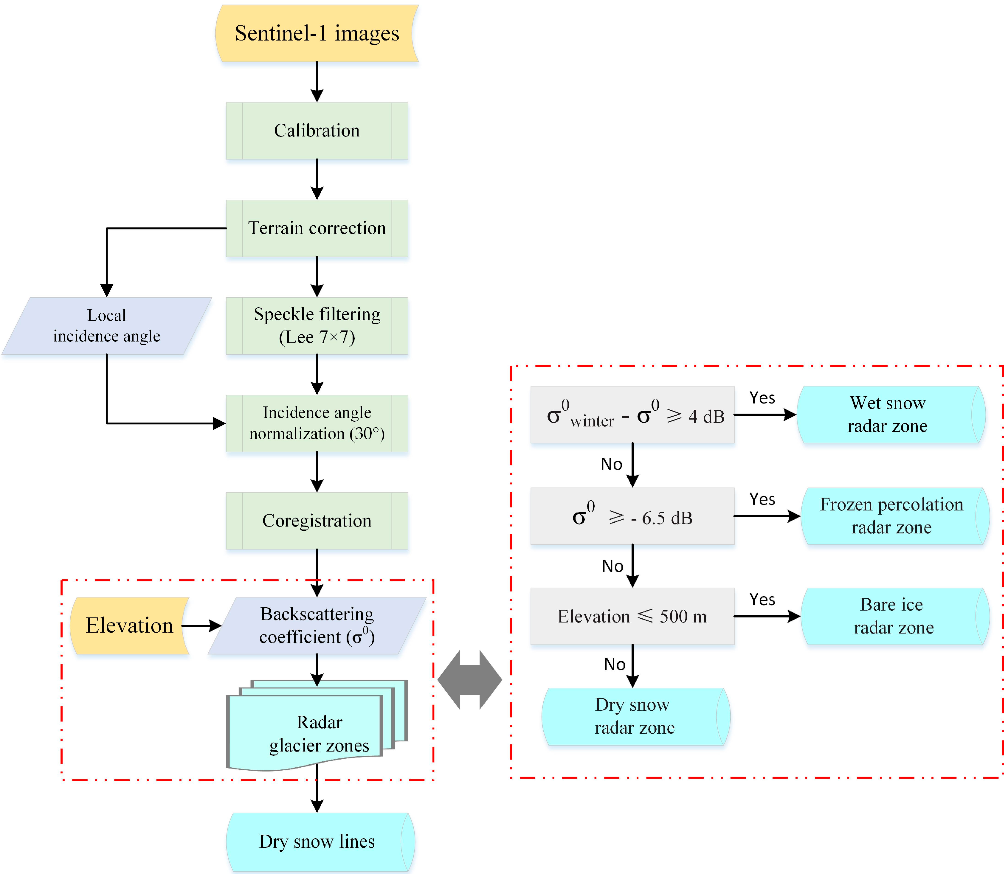
The differences in liquid snow content, snow grain size, and the relative elevations enable us to classify the RGZs based on Sentinel-1 SAR images. For the C-band Sentinel-1 images normalized to 30° incidence angle, the locations with σ0 4 dB lower than the winter observations were defined as wet snow radar zone. The brightest parts on the images (σ0 ≥ −6.5 dB) were categorized as frozen percolation radar zone. The rest of the dark patches above and below 500 m were classified as dry snow and bare ice radar zone, respectively. The flowchart for Sentinel-1 SAR image processing and rules for RGZ classification are shown in Figure 5.
4. Results
4.1. Melting Days in the AP
The winter mean SSM/I 19.35 GHz Tb in horizontal polarization varied greatly over the AP (Figure 6a). A melting day was counted when either Tb of the ascending and descending orbits pass beyond the thresholds. Heavy snowmelt was found on the Larsen Ice Shelf and Alexander Island (melting for more than two months), whereas the mountainous area of Palmer Land was frozen (Figure 6b). We also noticed that the places with long melting seasons show lower winter Tb compared with the frozen area. During refreezing, equitemperature metamorphosis results in coarse snow grains in places with a long melting season [60], leading to the stronger scattering and lower Tb compared with the places frozen all year around. As discussed in Section 3, meltwater refrozen in snowpacks also alters the morphological features, resulting in different backscattering characteristics in cold seasons.
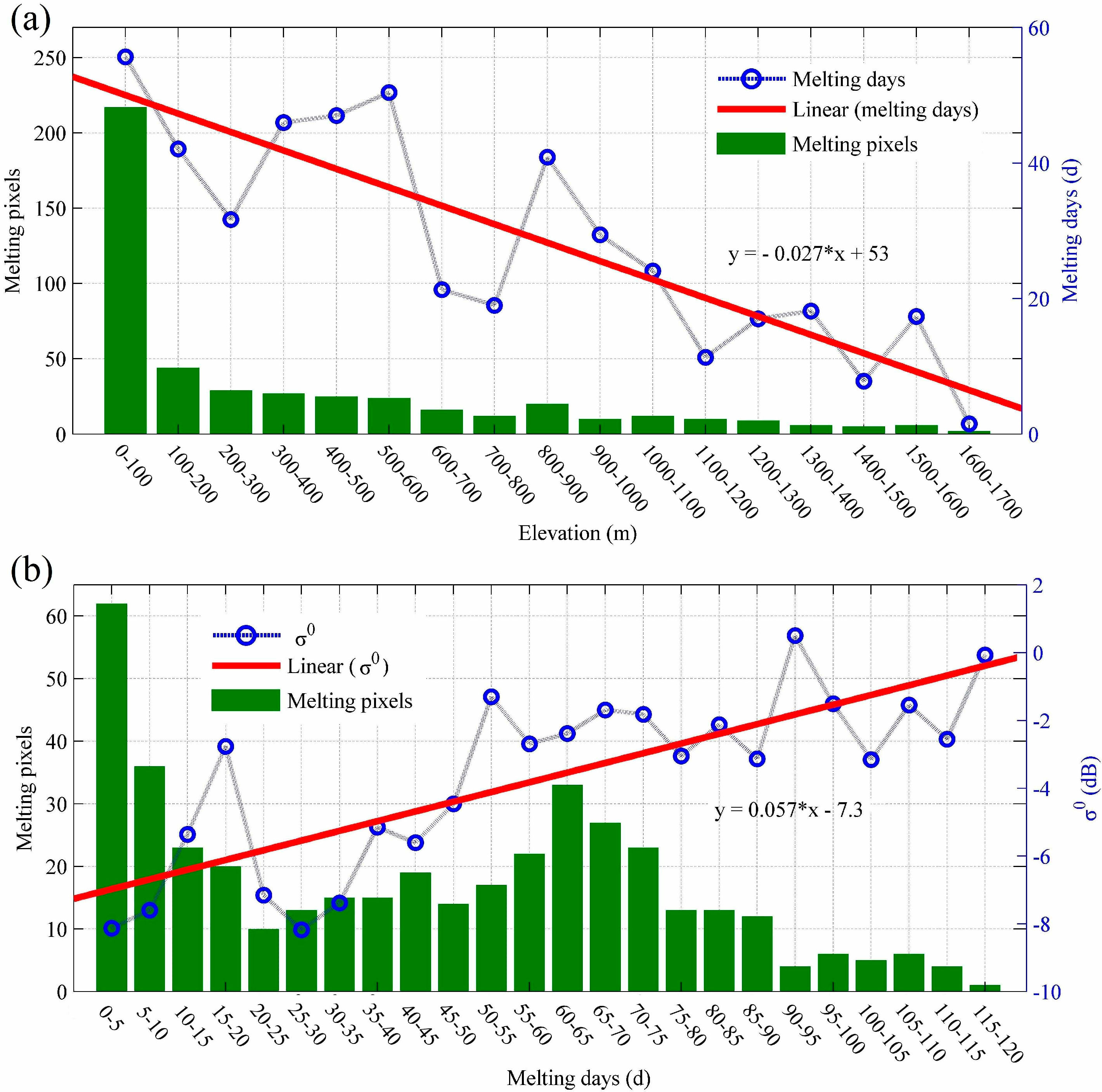
We calculated the mean melting days at 100 m elevation intervals. As shown in Figure 7a, mean melting days decreased with the increase in elevations. The correlation coefficient is −0.85. No melting signal was detected over 1700 m. The frequency of melting days showed two peaks, which represented short (0–5 days) and intense (60–65 days) melt seasons, respectively. Using the calibrated Sentinel-1 images listed in the left column of Table 1, we produced a winter mosaic of the AP from May to July in 2015 (Figure 6c). Figure 7b shows a comparison between the melting days derived from SSM/I data and σ0 derived from the winter Sentinel-1 mosaic. The Sentinel mosaic was resampled to the same size as the SSM/I data. We calculated the mean winter σ0 for every five melting days. The places with more melting days were much brighter on SAR images. The correlation coefficient is 0.78. This trend was significant for the areas where snowmelt lasts for less than 50 days, but not significant for the heavy melting places. Surface snowmelt led to the formation of ice layers and coarse grains in cold seasons, resulting in increased backscatter energy. The result supports the simulations of the frozen percolation radar zone in Section 3.2.
4.2. Mapping of RGZs
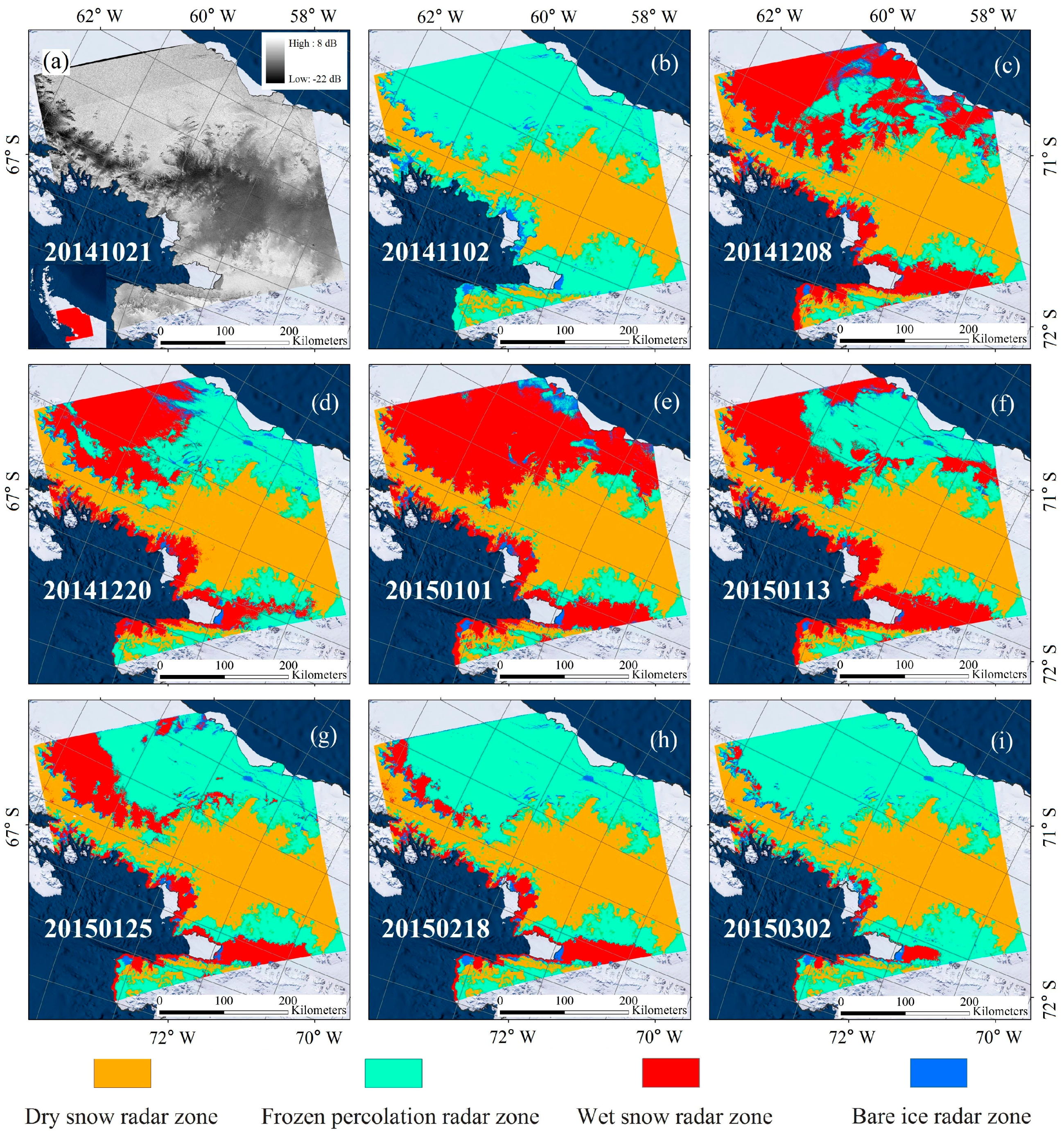
Based on the image preprocessing procedures and decision tree illuminated in Figure 5, RGZs in the middle of the AP were mapped by using the nine images listed in the right column of Table 1. These images observed the AP in the melting season from 21 October 2014 to 2 March 2015, covering the southern Larsen C Ice Shelf and Graham Land, the George VI Ice Shelf, and the north part of Palmer Land. Compared with the subsequent images, no snowmelt was interpreted on the image taken on 21 October (Figure 8a). This image served as a reference data for the detection of the wet snow radar zone, considering the absence of the earlier image.
Sentinel-1 images are effective for the interpretations of RGZs in the AP. The RGZs of this region were mapped, and are shown in Figure 8b–i. The middle AP was frozen at the beginning of November. Dry snow and frozen percolation radar zones dominated the mountains and ice shelves, respectively. Bare ice was sporadically distributed in the foothills and the edges of ice shelves (Figure 8a). Snowmelt (red area) expanded quickly in December. Most of the Larsen C and George VI ice shelves were melting at this time (Figure 8b,c). These ice shelves and the coastal areas beside the Bellingshausen Sea were almost totally melting on 1 January of the following year. Melt area retreated from the coastline to the piedmont region of the Graham Land from January to February (Figure 8e–h). The grounding zone of the Larsen C Ice Shelf showed the longest melting season. This phenomenon is consistent with the melting days, as shown in Figure 6b. The middle AP almost refroze on 2 May, except for some small patches distributed along the coastline beside the Bellingshausen Sea (Figure 8i). The wet snow radar zone and frozen percolation radar zone waxed and waned in the freeze–thaw cycle, but the dry snow radar zone remained unchanged the entire time.
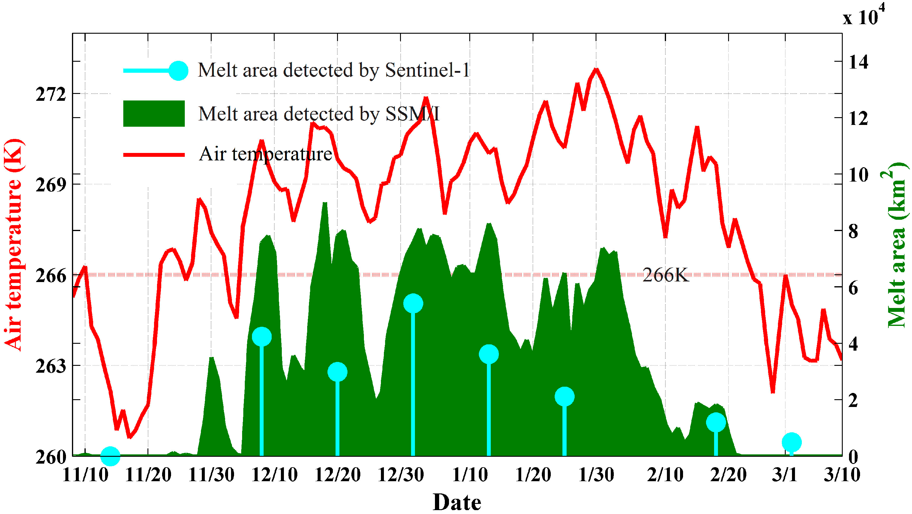
We compared the melt area detected by Sentinel-1 and the SSM/I with the ERA-Interim 2 m air temperature derived from the European Center for Medium-Range Weather Forecasting (http://www.ecmwf.int/). Melting signals were recognized by remote sensing techniques when the mean air temperature rose above 266 K (Figure 9). Melt area varied greatly with air temperature in the melting season. Wet snow radar zone detected by Sentinel-1 was smaller than the melt area derived from the SSM/I. When Sentinel-1 images were avaliable, the mean melt area identified by Sentinel-1 and the SSM/I was 2.89 × 10⁴ km2 and 5.64 × 10⁴ km2, respectively.
4.3. Mapping of DSL
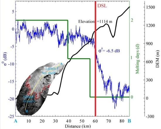
As the uppermost limit of the frozen percolation radar zone, the DSL’s position can shift significantly due to heavy snowmelt in summer. With the low temperatures in winter, very sporadic snowmelt was detected by the SSM/I in the coastal regions, indicating a stable position of winter DSL in the AP. On SAR images, the boundary between the frozen percolation and dry snow radar zone is seen as a transition from bright to dark. In Figure 10, we compared winter σ0, melting days, and the elevation of a profile across the Larsen G Ice Shelf and the upstream Swan Glacier (the green star shown in Figure 6c). Backscatter decreased significantly with the increase in elevation. SSM/I-derived melting days changed from two days to zero in the same time, indicating a summer with weak snowmelt. Backscatter was strong on the Larsen F Ice Shelf, and plummeted (under −6.5 dB) when the elevation increases above 1114 m. The σ0 decreased to −15 dB rapidly in places where no summer snowmelt was experienced. The clear boundary of the transition is the winter DSL, and the DSL elevation of profile AB is 1114 m.
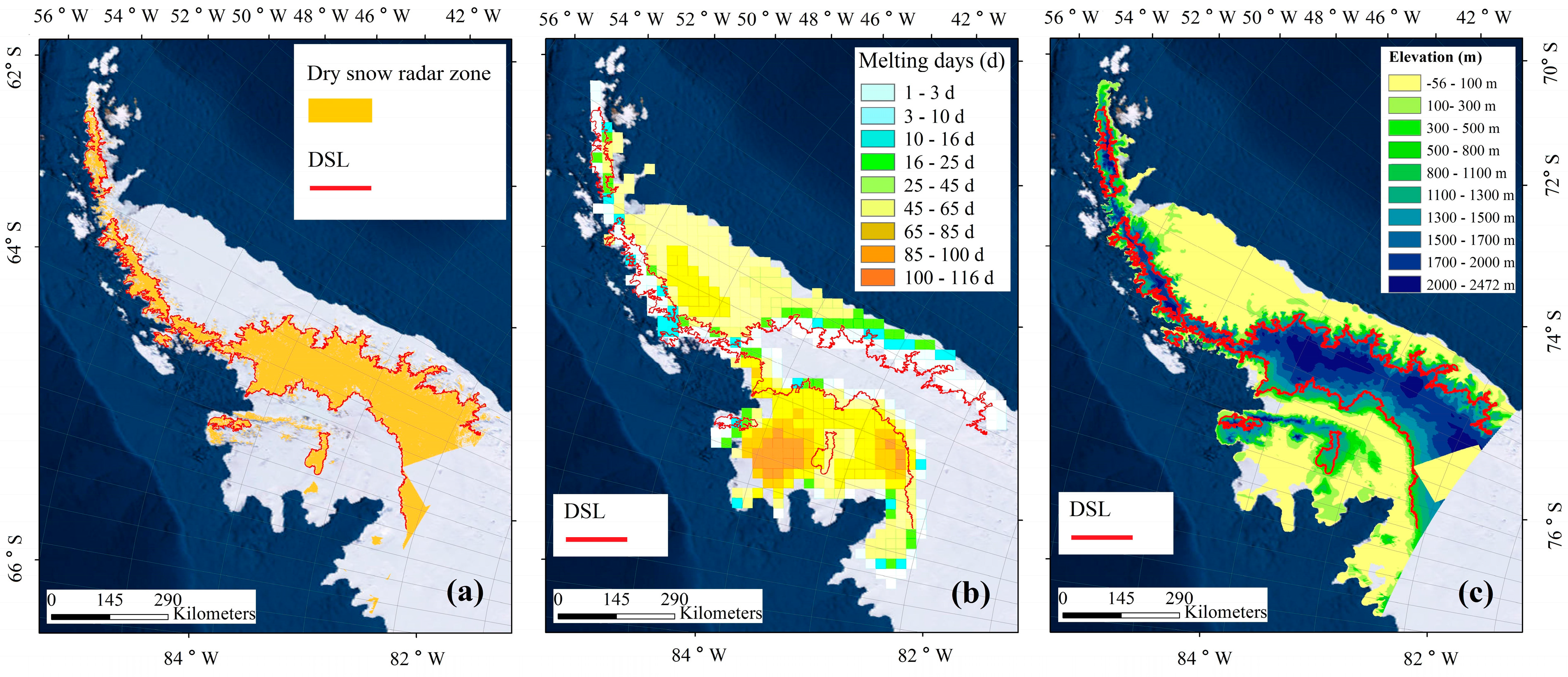
DSL in the AP was mapped by using the winter Sentinel-1 mosaic. Dry snow radar zones were mapped based on the decision tree. After clustering based on the classification aggregation in the ENVI software, the boundary of the dry snow patches larger than 25 km2 was extracted. The dry snow radar zone and DSL are shown in Figure 11a. Very good agreement was found between the dry snow regions detected by SAR and radiometer (Figure 11b). Compared with the melting days derived by SSM/I, DSL is mainly distributed in the areas melted for one to three days in summer, suggesting that the SSM/I recognized a slightly larger melt area. DSL distributed along the mountainside varied with latitudes and elevations, especially for the Palmer Land (Figure 11c).
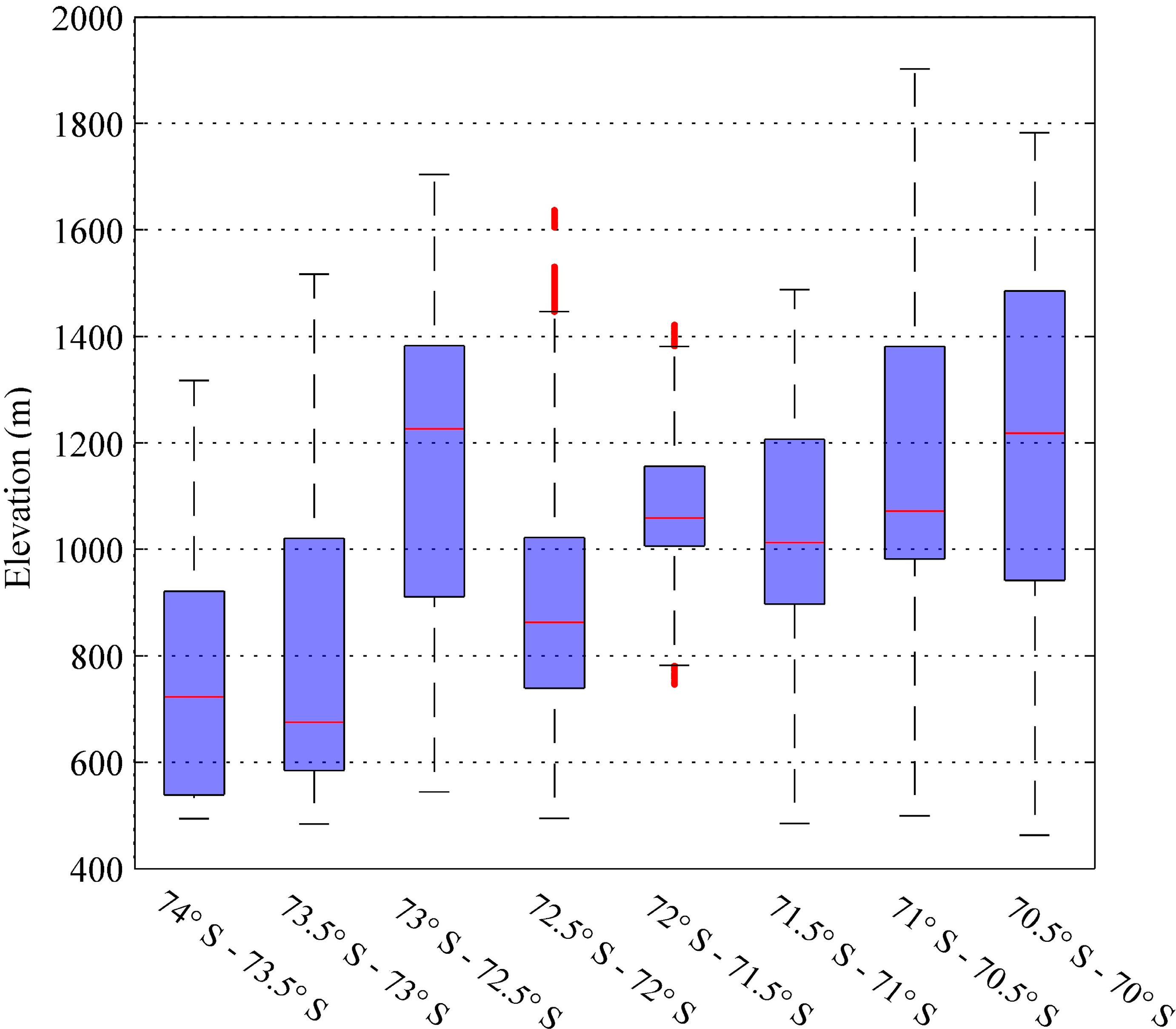
DSL agreed well with contour lines locally, but DSL elevations varied with the latitudes. The mean elevations of the DSL of the Palmer Land were calculated at a 0.5° interval of latitude from 74° S to 70° S. As shown in Figure 12, DSL elevations increased from south to north.
5. Discussion
Simulations of MEMLS3&a suggest that C-band σ0 with the incidence angle of 30° in wet snowpacks decreased for at least 4 dB compared with dry snow regime in the AP. The threshold is close to the value of 3 dB, which has been successfully used in Radarsat and ERS [32,61]. Horizontally polarized σ0 increases and decreases with snow depth in coarse-grained and fine-grained snowpacks, indicating a clear boundary between frozen percolation and dry snow radar zones. The transition from bright to dark can be easily recognized at a threshold of −6.5 dB, according to the simulations (Figure 4). This value agrees well with −6 dB used in Rau et al. (2000)’s work in the AP [62]. Backscatter decreases quickly from the frozen percolation to dry snow zone because of the differences in snow structure. As can be seen in Figure 10, σ0 drops rapidly from −5 dB to −10 dB in the transition, suggesting that the threshold is reasonable within a range. A lower threshold of −8 dB was used by Arigony–Neto et al. [8,34]. The result was supported by the higher winter σ0 with the increased summer melting days derived by SSM/I data (see in Figure 7b and Figure 10). However, this trend is not significant when the number of summer melting days is higher than 50, which may result from the increase of specular reflections from ice-saturated firn layers in winter [63]. The model error of MEMLS3&a, and some assumptions we made, may lead to the uncertainties in the simulations. For example, the model assumes that the layer interfaces are smooth. Some empirical parameters in the model also need further verification [51,53]. In the AP, snow profiles are much more complex than what we set in the simulations.
RGZs were classified on SAR images based on their differences in the liquid snow content, snow grain size, and the relative elevations. The temporal and spatial distributions of RGZs in the middle of the AP were mapped based on nine repeat-pass Sentinel-1 images. Compared with snowmelt detected by radiometer, the SAR-derived melting signals show a great improvement of spatial resolution, and can show detailed patterns of snowmelt. Snowmelt expanded from the grounding zone of the Larsen C Ice Shelf to the coastal area, but from the coastal area to the inland for the George VI Ice Shelf. The phenomenon agreed well with the melting days calculated from SSM/I data (Figure 6b). Föhn winds may explain the relatively long melting seasons in the western Larsen C Ice Shelf (Figure 6b and Figure 8). Low relative humidity of the air mass makes snowmelt or sublimation easier due to the adiabatically-dried föhn winds on the east side of the AP, leading to its ponding and thinning [32,64].
The wet snow radar zone detected by Sentinel-1 was smaller than the melt area derived from SSM/I data for several reasons. More extensive snowmelt was recognized by the SSM/I because of the dual observations. The much coarser spatial resolution of the SSM/I data also matters. A melt area of 625 km2 may be counted when only a small patch in the SSM/I pixel experiences snowmelt. The melting thin snow in periods of higher air temperatures would expose bare ice [65], leading to the underestimate of melt area on SAR images.
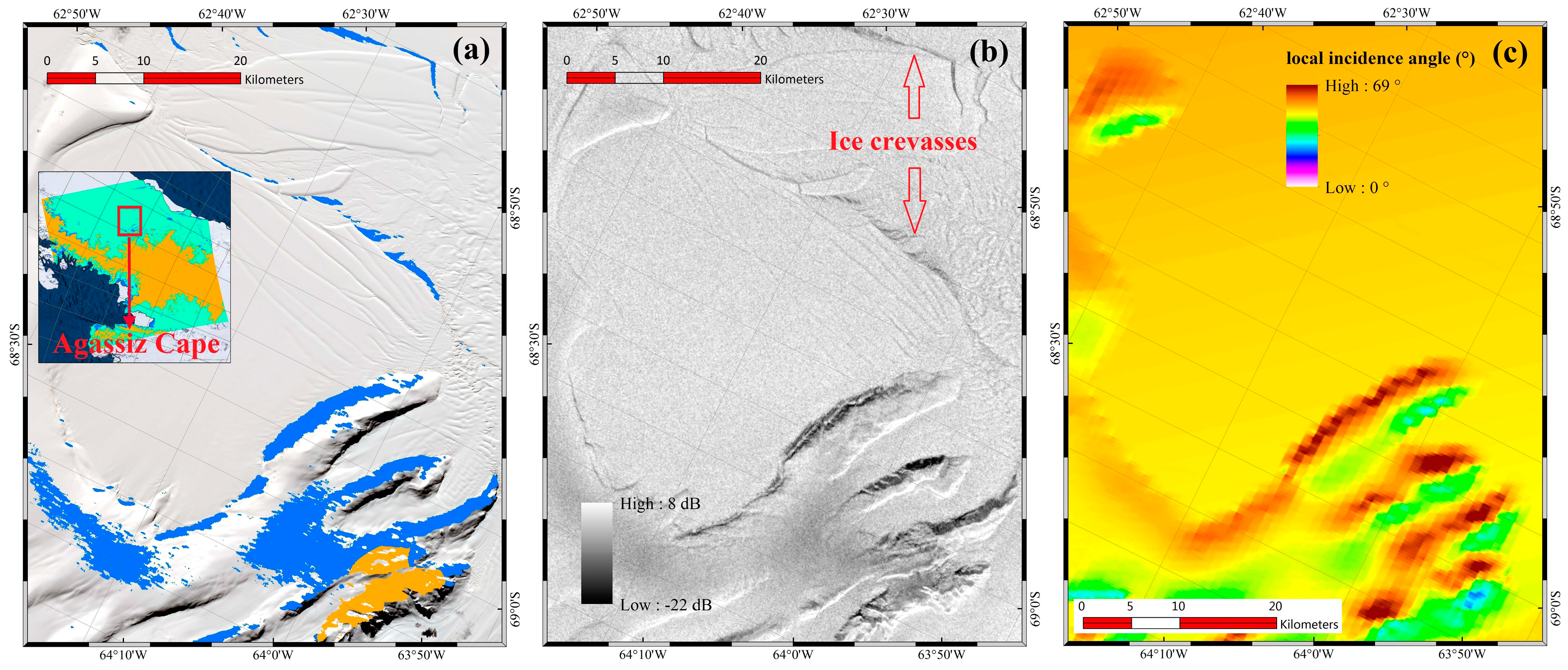
Minor misclassifications of RGZs exist in our study because of the special imaging mode of SAR. Figure 13a shows the misclassifications of the crevasses and mountains in Agassiz Cape on 14 November 2015. Crevasses with weak backscatter returns on ice shelves may be mistaken for bare ice (Figure 13b). Similarly, for the mountainous areas, the very high local incidence angles of the back slopes in the range direction lead to much lower σ0 (Figure 13c). These places were mistaken for bare ice or dry snow with the elevations below or above 500 m. It is also difficult to map the DSL in glaciers flowing through narrow valleys [34]. We hope that the addition of SAR textural features in future studies can help eliminate these misjudgments.
As the highest limit of snowmelt, winter DSL in the AP was mapped based on the SAR mosaic. DSL mainly distributed in the areas melted for one to three days in summer, indicating that a slightly larger accumulative summer melt area was recognized by the SSM/I. The largest dry snow patch was located on the Palmer Land, where the DSL elevations increased from south to north. Higher temperatures at the lower latitudes enable snowmelt to reach the higher altitudes.
6. Conclusions
This work develops a method to study the detailed melt pattern in the AP by using Sentinel-1 imagery. Based on a practical method of RGZ classification introduced in this study, the two open access Sentinel-1 satellites can provide timely accessible RGZs, as well as a way to study the dynamic changes in the detailed patterns of snowmelt at a spatial resolution of 40 m. The variances of DSL suggest the occurrences of heavy snowmelt in the AP, indicating the extreme events of polar climate. RGZ and DSL mapped by Sentinel-1 in this study are not validated directly because of the lack of in situ observations. However, the results agree well with the snowmelt detected by the SSM/I. In view of the dramatic collapses of the Larsen A and B ice shelves, the strong rising trend of the surface snowmelt threatens the stabilities of the ice shelves in the AP. With the subsequent launches of Sentinel 1C and 1D, RGZs and DSL detected by Sentinel-1 can reveal the exhaustive melting condition in the AP, and also provide input and output validations for the climate models.
Acknowledgments
The authors would like to thank the European Space Agency and the National Snow and Ice Data Center for providing the Sentinel-1 images and SSM/I brightness temperature data respectively. We also thank Martin Proksch (University of Innsbruck) for providing consultations on the MEMLS3&a. This research was supported in part by the National Natural Science Foundation of China (NSFC) (Grant no. 41531069 and 41376187) and in part by the Chinese Polar Environment Comprehensive Investigation & Assessment Programme (CHINARE2017-02-05).
Author Contributions
Chunxia Zhou and Lei Zheng conceived the study and carried out the design of the method. Chunxia Zhou processed the Sentinel-1 SAR images and conducted the manuscript preparation. Lei Zheng processed the SSM/I data and revised the manuscript.
Conflicts of Interest
The authors declare no conflict of interest.
References
- Steffen, K. Surface energy exchange at the equilibrium line on the Greenland ice sheet during onset of melt. Ann. Galciol. 1995, 21, 13–18. [Google Scholar] [CrossRef]
- Forster, R.R.; Isacks, B.L.; Das, S.B. Shuttle imaging radar (SIR-C/X-SAR) reveals near-surface properties of the South Patagonian Icefield. J. Geophys. Res. 1996, 101, 169–180. [Google Scholar] [CrossRef]
- Mortin, J.; Schrøder, T.M.; Hansen, A.W.; Holt, B.; Mcdonald, K.C. Mapping of seasonal freeze-thaw transitions across the pan-Arctic land and sea ice domains with satellite radar. J. Geophys. Res. 2012, 117, 1–19. [Google Scholar] [CrossRef]
- Hattermann, T.; Levermann, A. Response of Southern Ocean circulation to global warming may enhance basal ice shelf melting around Antarctica. Clim. Dyn. 2010, 35, 741–756. [Google Scholar] [CrossRef]
- Vaughan, D.G.; Marshall, G.J.; Connolley, W.M.; Parkinson, C.; Mulvaney, R.; Hodgson, D.A.; King, J.C.; Pudsey, C.J.; Turner, J. Recent rapid regional climate warming on the Antarctic Peninsula. Clim. Chang. 2003, 60, 243–274. [Google Scholar] [CrossRef]
- Zwally, H.J.; Fiegles, S. Extent and duration of Antarctic surface melting. J. Glaciol. 1994, 40, 463–476. [Google Scholar] [CrossRef]
- Tedesco, M.; Abdalati, W.; Zwally, H.J. Persistent surface snowmelt over Antarctica (1987–2006) from 19.35 GHz brightness temperatures. Geophys. Res. Lett. 2007, 34, 1–6. [Google Scholar] [CrossRef]
- Arigony-Neto, J.; Saurer, H.; Simões, J.C.; Rau, F.; Jaña, R.; Vogt, S.; Gossmann, H. Spatial and temporal changes in dry-snow line altitude on the Antarctic Peninsula. Clim. Chang. 2009, 94, 19–33. [Google Scholar] [CrossRef]
- Trusel, L.D.; Frey, K.E.; Das, S.B. Antarctic surface melting dynamics: Enhanced perspectives from radar scatterometer data. J. Geophys. Res. 2012, 117, 1–15. [Google Scholar] [CrossRef]
- Ashcraft, I.S.; Long, D.G. Comparison of methods for melt detection over Greenland using active and passive microwave measurements. Int. J. Remote Sens. 2006, 27, 2469–2488. [Google Scholar] [CrossRef]
- Liu, H.; Wang, L.; Jezek, K.C. Spatiotemporal variations of snowmelt in Antarctica derived from satellite scanning multichannel microwave radiometer and Special Sensor Microwave Imager data (1978–2004). J. Geophys. Res. 2006, 111, 1–20. [Google Scholar] [CrossRef]
- Wismann, V. Monitoring of seasonal snowmelt on greenland with ERS scatterometer data. IEEE Trans. Geosci. Remote Sens. 2000, 38, 1821–1826. [Google Scholar] [CrossRef]
- Picard, G.; Fily, M. Surface melting observations in Antarctica by microwave radiometers: Correcting 26-year time series from changes in acquisition hours. Remote Sens. Environ. 2006, 104, 325–336. [Google Scholar] [CrossRef]
- Liang, L.; Guo, H.; Li, X.; Cheng, X. Automated ice-sheet snowmelt detection using microwave radiometer measurements. Polar Res. 2013, 32, 89–99. [Google Scholar] [CrossRef]
- Bothale, R.V.; Rao, P.V.N.; Dutt, C.B.S.; Dadhwal, V.K.; Maurya, D. Spatio-temporal dynamics of surface melting over Antarctica using OSCAT and QuikSCAT scatterometer data (2001–2014). Curr. Sci. 2015, 109, 733–744. [Google Scholar]
- Liu, H.; Wang, L.; Jezek, K.C. Wavelet-transform based edge detection approach to derivation of snowmelt onset, end and duration from satellite passive microwave measurements. Int. J. Remote Sens. 2005, 26, 4639–4660. [Google Scholar] [CrossRef]
- Steiner, N.; Tedesco, M. A wavelet melt detection algorithm applied to enhanced-resolution scatterometer data over Antarctica (2000–2009). Cryosphere 2014, 8, 25–40. [Google Scholar] [CrossRef]
- Benson, C.S. Stratigraphic Studies in the Snow and Firn of the Greenland Ice Sheet; Research Report 70; Reprinted August 1996; U.S. Army Snow, Ice and Permafrost Research Establishment: Hanover, Germany, 1962. [Google Scholar]
- Rau, F.; Braun, M.; Friedrich, M.; Weber, F.; Goßmann, H. Radar glacier zones and their boundaries as indicators of glacier mass balance and climatic variability. In Proceedings of the 2nd EARSeL Workshop-Special Interest Group Land Ice and Snow, Dresden, Germany, 16–17 June 2000; pp. 317–327. [Google Scholar]
- Braun, M.; Rau, F.; Saurer, H.; Goßmann, H. Development of radar glacier zones on the King George Island ice cap, Antarctica, during austral summer 1996/97 as observed in ERS-2 SAR data. Ann. Galciol. 2000, 31, 357–363. [Google Scholar] [CrossRef]
- Ramage, J.M.; Isacks, B.L.; Miller, M.M. Radar glacier zones in southeast Alaska, USA: Field and satellite observations. J. Glaciol. 2000, 46, 287–296. [Google Scholar] [CrossRef]
- Langley, K.; Hamran, S.E.; Hogda, K.A.; Storvold, R.; Brandt, O.; Kohler, J.; Hagen, J.O. From glacier facies to SAR backscatter zones via GPR. IEEE Trans. Geosci. Remote Sens. 2008, 46, 2506–2516. [Google Scholar] [CrossRef]
- Huang, L.; Li, Z.; Tian, B.; Chen, Q.; Zhou, J. Monitoring glacier zones and snow/firn line changes in the Qinghai–Tibetan Plateau using C-band SAR imagery. Remote Sens. Environ. 2013, 137, 17–30. [Google Scholar] [CrossRef]
- Kundu, S.; Chakraborty, M. Delineation of glacial zones of Gangotri and other glaciers of Central Himalaya using RISAT-1 C-band dual-pol SAR. Int. J. Remote Sens. 2015, 36, 1529–1550. [Google Scholar] [CrossRef]
- Baghdadi, N.; Gauthier, Y.; Bernier, M. Capability of multitemporal ERS-1 sar data for wet-snow mapping. Remote Sens. Environ. 1997, 60, 174–186. [Google Scholar] [CrossRef]
- Magagi, R.; Bernier, M. Optimal conditions for wet snow detection using RADARSAT SAR data. Remote Sens. Environ. 2003, 84, 221–233. [Google Scholar] [CrossRef]
- Usami, N.; Muhuri, A.; Bhattacharya, A.; Hirose, A. POLSAR wet snow mapping with incidence angle information. IEEE Trans. Geosci. Remote Sens. Lett. 2016, 13, 2029–2033. [Google Scholar] [CrossRef]
- He, G.; Feng, X.; Xiao, P.; Xia, Z.; Wang, Z.; Chen, H.; Hui, L.; Guo, J. Dry and wet snow cover mapping in mountain areas using SAR and optical remote sensing data. IEEE J. Sel. Top. Appl. Earth Obs. Remote Sens. 2017, 10, 2575–2588. [Google Scholar] [CrossRef]
- Tian, B.; Li, Z.; Zhu, Y. Terrain correction of polarimetric sar data and its application in mapping mountain glacier facies with RADARSAT-2 SAR. ISPRS Int. Arch. Photogramm. Remote Sens. Spat. Inf. Sci. 2011, 3819, 319–324. [Google Scholar] [CrossRef]
- Akbari, V.; Doulgeris, A.; Eltoft, T. Non-Gaussian clustering of SAR images for glacier change detection. In Proceedings of the ESA Living Planet Symposium, Bergen, Norway, 28 June–2 July 2010. [Google Scholar]
- Rizzoli, P.; Martone, M.; Rott, H.; Moreira, A. Characterization of snow facies on the Greenland Ice Sheet observed by TanDEM-X interferometric SAR data. Remote Sens. 2017, 9, 315. [Google Scholar] [CrossRef]
- Luckman, A.; Elvidge, A.; Jansen, D.; Kulessa, B.; Kuipers Munneke, P.; King, J.; Barrand, N.E. Surface melt and ponding on Larsen C Ice Shelf and the impact of föhn winds. Antarct. Sci. 2014, 26, 625–635. [Google Scholar] [CrossRef] [Green Version]
- Rau, F. The Upward Shift of Dry Snow Line on the Northern Antarctic Peninsula. In Proceedings of the EARSel-LISSIG-Workshop Observing our Cryosphere from Space, Bern, Switzerland, 11–13 March 2002. [Google Scholar]
- Arigony-Neto, J.; Rau, F.; Saurer, H.; Jaña, R.; Simöes, J.C.; Vogt, S. A time series of SAR data for monitoring changes in boundaries of glacier zones on the Antarctic Peninsula. Ann. Galciol. 2007, 46, 55–60. [Google Scholar] [CrossRef]
- Fahnestock, M.A.; Abdalati, W.; Shuman, C.A. Long melt seasons on ice shelves of the Antarctic Peninsula: An analysis using satellite-based microwave emission measurements. Ann. Galciol. 2001, 34, 127–133. [Google Scholar] [CrossRef]
- Vaughan, D.G. Recent trends in melting conditions on the Antarctic Peninsula and their implications for ice-sheet mass balance and sea level. Arct. Antarct. Alp. Res. 2006, 38, 147–152. [Google Scholar] [CrossRef]
- Alley, K.E.; Scambos, T.A.; Siegfried, M.R.; Fricker, H.A. Impacts of warm water on Antarctic ice shelf stability through basal channel formation. Nat. Geosci. 2016, 9, 290–293. [Google Scholar] [CrossRef]
- Van den Broeke, M. Strong surface melting preceded collapse of Antarctic Peninsula ice shelf. Geophys. Res. Lett. 2005, 32, 273–280. [Google Scholar] [CrossRef]
- Steffen, K.; Abdalati, W.; Stroeve, J. Climate sensitivity studies of the Greenland ice sheet using satellite AVHRR, SMMR, SSM/I and in situ data. Meteorol. Atmos. Phys. 1993, 51, 239–258. [Google Scholar] [CrossRef]
- Abdalati, W.; Steffen, K. Snowmelt on the Greenland Ice Sheet as derived from passive microwave satellite data. J. Clim. 1997, 10, 165–175. [Google Scholar] [CrossRef]
- Fettweis, X.; van Ypersele, J.P.; Gallée, H.; Lefebre, F.; Lefebvre, W. The 1979–2005 Greenland ice sheet melt extent from passive microwave data using an improved version of the melt retrieval XPGR algorithm. Geophys. Res. Lett. 2007, 34, 247–260. [Google Scholar] [CrossRef]
- Armstrong, R.L.; Knowles, K.W.; Brodzik, M.J.; Hardman, M.A. DMSP SSM/I-SSMIS Pathfinder Daily EASE-Grid Brightness Temperatures, Version 2; National Snow and Ice Data Center (NSIDC): Boulder, CO, USA, 1994. [Google Scholar]
- Torres, R.; Snoeij, P.; Geudtner, D.; Bibby, D.; Davidson, M.; Attema, E.; Potin, P.; Rommen, B.; Floury, N.; Brown, M.; et al. GMES Sentinel-1 mission. Remote Sens. Environ. 2012, 120, 9–24. [Google Scholar] [CrossRef]
- Nagler, T.; Rott, H.; Ripper, E.; Bippus, G.; Hetzenecker, M. Advancements for Snowmelt Monitoring by Means of Sentinel-1 SAR. Remote Sens. 2016, 8, 348. [Google Scholar] [CrossRef]
- Mladenova, I.E.; Jackson, T.J.; Bindlish, R.; Hensley, S. Incidence angle normalization of radar backscatter data. IEEE Trans. Geosci. Remote Sens. 2013, 51, 1791–1804. [Google Scholar] [CrossRef]
- Topouzelis, K.; Singha, S.; Kitsiou, D. Incidence angle normalization of Wide Swath SAR data for oceanographic applications. Open Geosci. 2016, 8, 450–464. [Google Scholar] [CrossRef]
- Tedesco, M. Assessment and development of snowmelt retrieval algorithms over Antarctica from K-band spaceborne brightness temperature (1979–2008). Remote Sens. Environ. 2009, 113, 979–997. [Google Scholar] [CrossRef]
- Langley, K.; Hamran, S.E.; Hogda, K.A.; Storvold, R.; Brandt, O.; Hagen, J.O.; Kohler, J. Use of C-band ground penetrating radar to determine backscatter sources within glaciers. IEEE Trans. Geosci. Remote Sens. 2007, 45, 1236–1246. [Google Scholar] [CrossRef]
- Smith, L.C.; Forster, R.R.; Isacks, B.L.; Hall, D.K. Seasonal climatic forcing of alpine glaciers revealed with orbital synthetic aperture radar. J. Glaciol. 1997, 43, 480–488. [Google Scholar] [CrossRef]
- Rignot, E.; Echelmeyer, K.; Krabill, W. Penetration depth of interferometric synthetic-aperture radar signals in snow and ice. Geophys. Res. Lett. 2001, 28, 3501–3504. [Google Scholar] [CrossRef]
- Proksch, M.; Mätzler, C.; Wiesmann, A.; Lemmetyinen, J.; Schwank, M.; Löwe, H.; Schneebeli, M. MEMLS3&a: Microwave emission model of layered snowpacks adapted to include backscattering. Geosci. Model Dev. 2015, 8, 2611–2626. [Google Scholar]
- Mätzler, C.; Wiesmann, A. Extension of the microwave emission model of layered snowpacks to coarse-grained snow. Remote Sens. Environ. 1999, 70, 317–325. [Google Scholar] [CrossRef]
- Wiesmann, A.; Mätzler, C. Microwave emission model of layered snowpacks. Remote Sens. Environ. 1999, 70, 307–316. [Google Scholar] [CrossRef]
- Skolnik, M.I. Radar Handbook, 2nd ed.; McGraw-Hill: New York, NY, USA, 1990; p. 86. [Google Scholar]
- Svendsen, E.; Kloster, K.; Farrelly, B.; Johannessen, O.M.; Johannessen, J.A.; Campbell, W.J.; Gloersen, P.; Cavalieri, D.; Mätzler, C. Norwegian Remote Sensing Experiment: Evaluation of the Nimbus 7 scanning multichannel microwave radiometer for sea ice research. J. Geophys. Res. 1983, 88, 2781–2791. [Google Scholar] [CrossRef]
- Mätzler, C. Relation between grain-size and correlation length of snow. J. Glaciol. 2002, 48, 461–466. [Google Scholar] [CrossRef]
- Dai, L.; Che, T.; Wang, J.; Zhang, P. Snow depth and snow water equivalent estimation from AMSR-E data based on a priori snow characteristics in Xinjiang, China. Remote Sens. Environ. 2012, 127, 14–29. [Google Scholar] [CrossRef]
- Hallikainen, M.; Ulaby, F.; Abdelrazik, M. Dielectric properties of snow in the 3 to 37 GHz range. IEEE Trans. Antennas Propag. 1986, 34, 1329–1340. [Google Scholar] [CrossRef]
- Korhonen, K. Microclimate in the snow burrows of willow grouse (Lagopus lagopus). Ann. Zool. Fenn. 1980, 17, 5–9. [Google Scholar]
- Markus, T.; Stroeve, J.C.; Miller, J. Recent changes in Arctic sea ice melt onset, freezeup, and melt season length. J. Geophys. Res. 2009, 114, 1–14. [Google Scholar] [CrossRef]
- Nagler, T.; Rott, H. Retrieval of wet snow by means of multitemporal SAR data. IEEE Trans. Geosci. Remote Sens. 2000, 38, 754–765. [Google Scholar] [CrossRef]
- Rau, F.; Braun, M.; Saurer, H.; Goßmann, H.; Kothe, G.; Weber, F.; Ebel, M.; Beppler, D. Monitoring multi-year snow cover dynamics on the Antarctic Peninsula using SAR imagery. Polarforschung 2000, 67, 27–40. [Google Scholar]
- Alley, K.E.; Scambos, T.A.; Long, D.G. Assessing Antarctica’s ice shelves for vulnerability to surface-melt-induced collapse using scatterometry. In Proceedings of the American Geophysical Union Fall Meeting, San Francisco, CA, USA, 15–19 December 2014. [Google Scholar]
- Trusel, L.D.; Frey, K.E.; Das, S.B.; Kuipers Munneke, P.; van den Broeke, M. Satellite-based estimates of Antarctic surface meltwater fluxes. Geophys. Res. Lett. 2013, 40, 6148–6153. [Google Scholar] [CrossRef]
- Hui, F.; Ci, T.; Cheng, X.; Scambos, T.A.; Liu, Y.; Zhang, Y.; Chi, Z.; Huang, H.; Wang, X.; Wang, F.; et al. Mapping blue-ice areas in Antarctica using ETM+ and MODIS data. Ann. Galciol. 2014, 55, 129–137. [Google Scholar] [CrossRef]
Figure 1.
Map of the Antarctic Peninsula (AP). (a) Location of the AP on Antarctica; (b) Digital elevation model (DEM) of the AP obtained from the National Snow and Ice Data Center (NSIDC, http://nsidc.org/). The black line is the boundary of the study area, and the colored rectangles are the frames of Sentinel-1 images used in this study. The base map was obtained from Earthstar Geographics (http://www.terracolor.net/).

Figure 2.
Ascending special sensor microwave/imager (SSM/I) 19.35 GHz Tb in the horizontal polarization of two pixels from July 2014 to June 2015. The red line represents a melting pixel with a threshold of 190 K (red dot line) on the Larsen C Ice Shelf. The green line represents a frozen pixel with a threshold of 232 K (green dot line) on Palmer Land.

Figure 3.
C-band σ0 changes with liquid water content simulated by MEMLS3&a. Incidence angle was set as 30°, and snow depth was set as 1, 10, 50, and 200 cm in (a–d) respectively. Simulations with snow density ranging from 350 kg/m3 to 540 kg/m3 and snow grain size ranging from 0.5 mm to 3 mm were conducted.

Figure 4.
C-band σ0 changes along with snow depth simulated by MEMLS3&a. Incidence angle was set as 30°, coarse-grained (3–8 mm) snowpacks and fine-grained (0.5–2 mm) snowpacks of different snow densities (350–540 kg/m3) were considered.
Figure 4.
C-band σ0 changes along with snow depth simulated by MEMLS3&a. Incidence angle was set as 30°, coarse-grained (3–8 mm) snowpacks and fine-grained (0.5–2 mm) snowpacks of different snow densities (350–540 kg/m3) were considered.
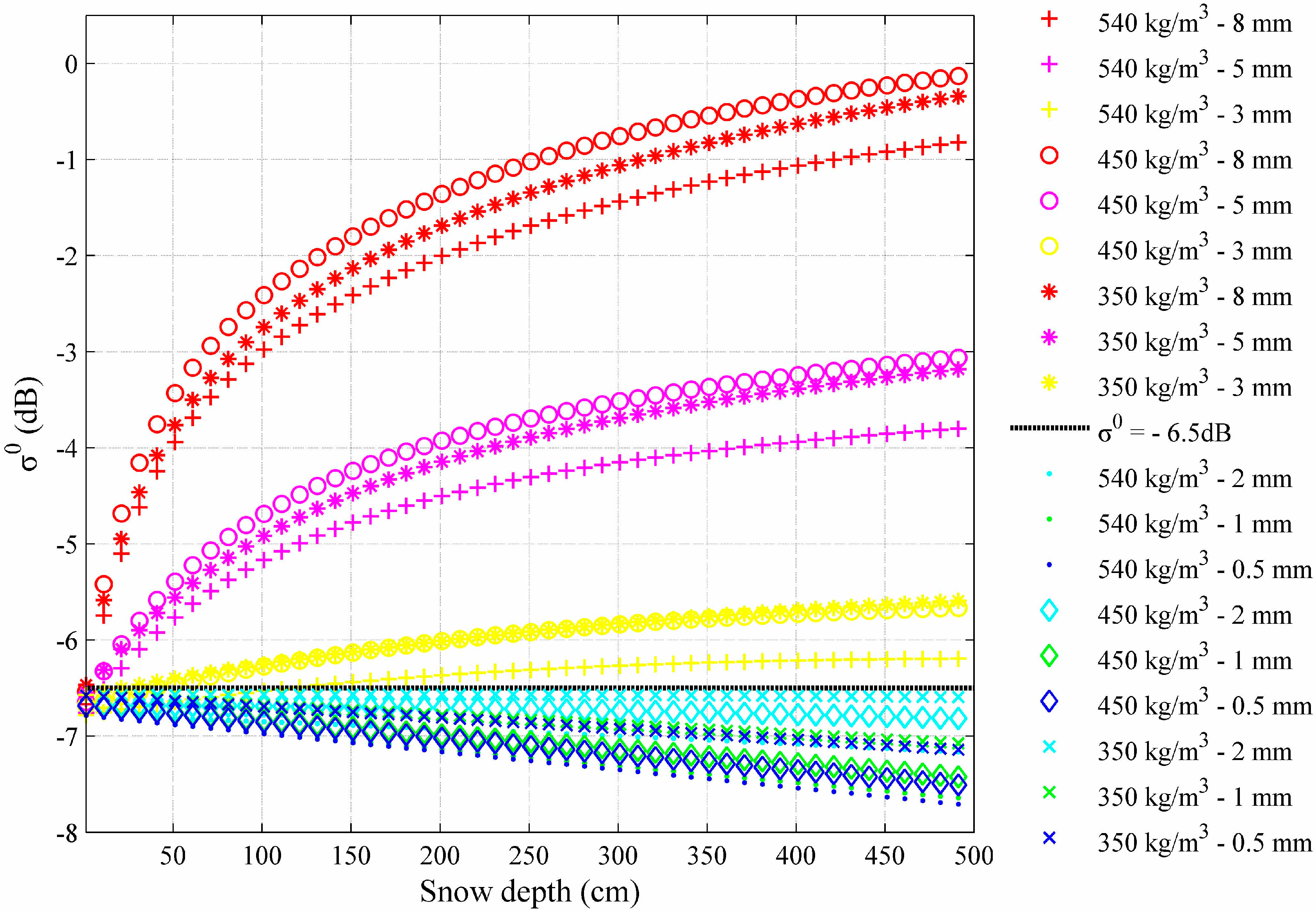
Figure 5.
Flowchart of the RGZ mapping with Sentinel-1 synthetic aperture radar (SAR) images.

Figure 6.
(a) Winter mean ascending SSM/I 19.35 GHz Tb in horizontal polarization. (b) Melting days over the AP derived from SSM/I data during 2014–2015. (c) Normalized radar backscatter of Sentinel-1 mosaic with the reference angle of 30°. The yellow star shows the location of the Larsen F Ice Shelf, and the upstream Swan Glacier.
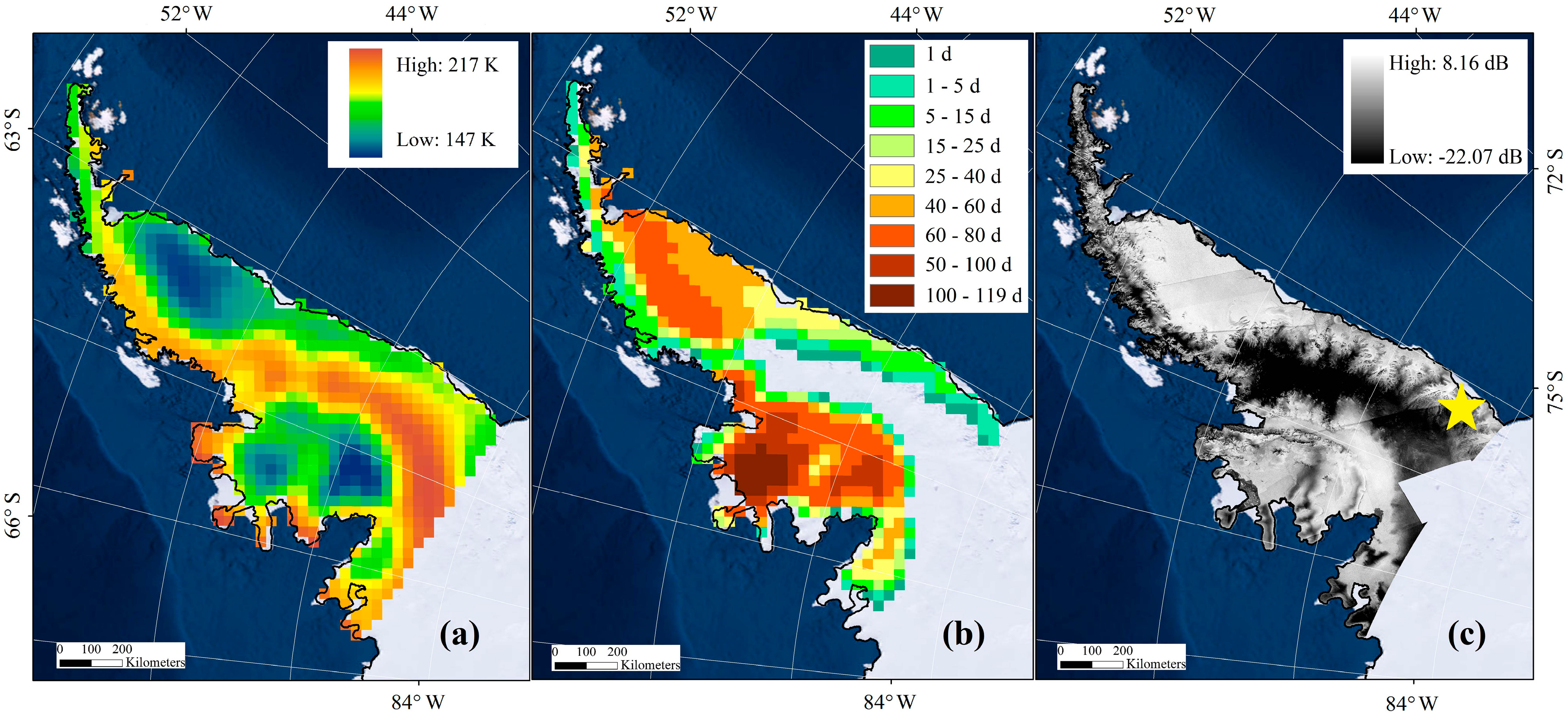
Figure 7.
Relationships between melting days, elevation, and backscatter. (a) shows the mean melting days at 100 m elevation intervals (blue empty dots). (b) shows the mean winter σ0 for every five melting days (blue empty dots). The red lines and green bars represent the linear trend and sample size, respectively.

Figure 8.
RGZs of the middle AP derived from Sentinel-1 images. (a) shows the reference image for mapping of the wet snow radar zone. The map on the bottom left shows the location of the images in the AP. (b–i) illustrate the dry snow (orange area), frozen percolation (cyan area), wet snow (red area), and bare ice radar zone (blue area) from 2 November 2014 to 2 March 2015.

Figure 9.
Comparison of 2-m air temperature (red solid line) and melt areas detected by Sentinel-1 (cyan stems) and the SSM/I (green areas). Melting signals were detected when mean air temperature rose above 266 K (red dotted line).
Figure 9.
Comparison of 2-m air temperature (red solid line) and melt areas detected by Sentinel-1 (cyan stems) and the SSM/I (green areas). Melting signals were detected when mean air temperature rose above 266 K (red dotted line).

Figure 10.
Winter σ0 (blue line), melting days (green line), and elevation (black line) along a profile across the Larsen F Ice Shelf and the upstream Swan Glacier (corresponding to the star in Figure 6c). The red line marks the location of the dry snow line (DSL). The backscatter map at the bottom left corner shows the route of profile AB (yellow line).

Figure 11.
(a) shows the dry snow radar zone (yellow area) and DSL (red line) derived by Sentinel-1. The DSL was overlapped with melting days and elevation in (b,c), respectively.
Figure 11.
(a) shows the dry snow radar zone (yellow area) and DSL (red line) derived by Sentinel-1. The DSL was overlapped with melting days and elevation in (b,c), respectively.

Figure 12.
Boxplot of the DSL elevations at a 0.5° interval of latitude on the Palmer land.

Figure 13.
Misclassifications of RGZs in Agassiz Cape on 14 November 2015. (a) shows the location of Agassiz Cape and the misclassifications of the crevasses and mountains. Blue and yellow areas represent bare ice and dry snow, respectively. The base map is a Landsat 8 image from 2 November 2015 derived from the United States Geological Survey (USGS, http://glovis.usgs.gov/). (b) illustrates the ice crevasses on the corresponding SAR image. (c) shows the local incidence angle.


Table 1.
Sentinel-1 images used in this study. RGZ: radar glacier zone.
| Images for the Winter Mosaic of the AP | Images for the RGZs Mapping | ||||
|---|---|---|---|---|---|
| Relative Orbit Number | Slice Number | Date | Relative Orbit Number | Slice Number | Date |
| 48 | 3 | 1 May 2015 | 48 | 4 | 21 October 2014 |
| 48 | 4 | 1 May 2015 | 48 | 4 | 2 November 2014 |
| 48 | 5 | 1 May 2015 | 48 | 4 | 8 December 2014 |
| 62 | 5 | 1 May 2015 | 48 | 4 | 20 December 2014 |
| 106 | 4 | 5 May 2015 | 48 | 4 | 1 January 2015 |
| 106 | 5 | 5 May 2015 | 48 | 4 | 13 January 2015 |
| 111 | 1 | 5 May 2015 | 48 | 4 | 25 January 2015 |
| 18 | 5 | 10 May 2015 | 48 | 4 | 18 February 2015 |
| 34 | 3 | 12 May 2015 | 48 | 4 | 2 March 2015 |
| 92 | 3 | 16 May 2015 | |||
| 96 | 0 | 16 May 2015 | |||
| 19 | 4 | 4 June 2015 | |||
| 165 | 1 | 20 July 2015 | |||
© 2017 by the authors. Licensee MDPI, Basel, Switzerland. This article is an open access article distributed under the terms and conditions of the Creative Commons Attribution (CC BY) license (http://creativecommons.org/licenses/by/4.0/).
Share and Cite
MDPI and ACS Style
Zhou, C.; Zheng, L. Mapping Radar Glacier Zones and Dry Snow Line in the Antarctic Peninsula Using Sentinel-1 Images. Remote Sens. 2017, 9, 1171. https://doi.org/10.3390/rs9111171
AMA Style
Zhou C, Zheng L. Mapping Radar Glacier Zones and Dry Snow Line in the Antarctic Peninsula Using Sentinel-1 Images. Remote Sensing. 2017; 9(11):1171. https://doi.org/10.3390/rs9111171
Chicago/Turabian StyleZhou, Chunxia, and Lei Zheng. 2017. "Mapping Radar Glacier Zones and Dry Snow Line in the Antarctic Peninsula Using Sentinel-1 Images" Remote Sensing 9, no. 11: 1171. https://doi.org/10.3390/rs9111171
Note that from the first issue of 2016, this journal uses article numbers instead of page numbers. See further details here.