Validation and Calibration of QAA Algorithm for CDOM Absorption Retrieval in the Changjiang (Yangtze) Estuarine and Coastal Waters


State Key Laboratory of Estuarine and Coastal Research, East China Normal University, 3663 Zhongshan N. Road, Shanghai 200062, China
*
Author to whom correspondence should be addressed.
Remote Sens. 2017, 9(11), 1192; https://doi.org/10.3390/rs9111192
Submission received: 29 August 2017
/
Revised: 9 November 2017
/
Accepted: 18 November 2017
/
Published: 21 November 2017
(This article belongs to the Special Issue Advancing Earth Surface Representation via Enhanced Use of Earth Observations in Monitoring and Forecasting Applications)
Abstract
:Distribution, migration and transformation of chromophoric dissolved organic matter (CDOM) in coastal waters are closely related to marine biogeochemical cycle. Ocean color remote sensing retrieval of CDOM absorption coefficient (ag(λ)) can be used as an indicator to trace the distribution and variation characteristics of the Changjiang diluted water, and further to help understand estuarine and coastal biogeochemical processes in large spatial and temporal scales. The quasi-analytical algorithm (QAA) has been widely applied to remote sensing inversions of optical and biogeochemical parameters in water bodies such as oceanic and coastal waters, however, whether the algorithm can be applicable to highly turbid waters (i.e., Changjiang estuarine and coastal waters) is still unknown. In this study, large amounts of in situ data accumulated in the Changjiang estuarine and coastal waters from 9 cruise campaigns during 2011 and 2015 are used to verify and calibrate the QAA. Furthermore, the QAA is remodified for CDOM retrieval by employing a CDOM algorithm (QAA_CDOM). Consequently, based on the QAA and the QAA_CDOM, we developed a new version of algorithm, named QAA_cj, which is more suitable for highly turbid waters, e.g., Changjiang estuarine and coastal waters, to decompose ag from adg (CDOM and non-pigmented particles absorption coefficient). By comparison of matchups between Geostationary Ocean Color Imager (GOCI) retrievals and in situ data, it reveals that the accuracy of retrievals from calibrated QAA is significantly improved. The root mean square error (RMSE), mean absolute relative error (MARE) and bias of total absorption coefficients (a(λ)) are lower than 1.17, 0.52 and 0.66 m−1, and ag(λ) at 443 nm are lower than 0.07, 0.42 and 0.018 m−1. These results indicate that the calibrated algorithm has a better applicability and prospect for highly turbid coastal waters with extremely complicated optical properties. Thus, reliable CDOM products from the improved QAA_cj can advance our understanding of the land-ocean interaction process by earth observations in monitoring spatial-temporal distribution of the river plume into sea.
1. Introduction
Remote sensing of oceans and coastal zones is a key technology for monitoring spatial-temporal distribution of the river plume into sea and understanding of the land-ocean interaction processes. Satellite retrievals of inherent optical parameters (IOPs) of waters such as absorption and scattering characteristics is one of the most important applications of ocean color remote sensing [1]. Furthermore, chlorophyll, chromophoric dissolved organic matter (CDOM), suspended sediment and other water component concentrations can be derived from IOPs, which leads to further estimations of phytoplankton biomass, primary productivity and heat flux [2]. The IOPs mainly include absorption coefficient (a(λ), see Table 1 for symbols and definitions) and backscattering coefficient. They are the source of the satellite remote sensing to quantify ocean water information [3], and key parameters of bio-optical models [4]. CDOM absorption coefficient is often used as a tracer to evaluate the amount of nutrients carried by Changjiang diluted water. Numerous applications of remote sensing have allowed to retrieve main components of water (i.e., phytoplankton, non-pigmented particles and CDOM) worldwide [5,6,7]. In CDOM-rich regions, such as North America and northern Europe, CDOM determines the optical properties of marine waters to a large extent and its existence can affect marine biogeochemical processes by the light absorption. Bricaud et al. [8] pointed out that even low concentrations of CDOM in the open sea may have an effect on absorption and hence on ocean color similar to that of low or moderate algal biomass; Nieke et al. [9] supported the possibility of using light absorption characteristics of CDOM in coastal waters strongly influenced by freshwater runoff in the Estuary and Gulf of St. Lawrence system (Canada); Darecki et al. [10] found a strong influence of CDOM absorption on the quantitative and qualitative features of spectral reflectance of in two different water bodies with similar chlorophyll content in the Baltic Sea; Hu et al. [11] estimated ag to study occurrence and distribution of red tides in coastal waters off South Florida; Bowers et al. [12] used salinity to determinate ag in an estuary for exploring the river discharge.
A number of algorithms were proposed to quantify ag(λ) from spectral measurements of ocean water. Empirical algorithms [13,14,15,16,17,18,19] were mostly based on spectral reflectance ratios to calculate ag(λ), and these algorithms required adequate data to parameterize the model and may only be valid for specific locations. Algorithms based on statistical modeling [18,20,21,22,23,24], such as optimization (Garver-Siegel-Maritorena, GSM), matrix inversion algorithm, artificial neural network (aNN) and Linear Matrix Inversion (LMI) algorithm, used some semi-analytical methodologies, but required knowledge about specific biochemical parameters [5]. Semi-analytical algorithms [25,26,27] mostly use Rrs(λ) to calculate IOPs and further to estimate biochemical parameters, which incorporate both empirical parameters and bio-optical models. The quasi-analytical algorithm (QAA) developed by Lee et al. [28] was widely applied during the last decade. Several updated versions were presented in following years [29,30,31]. Recent version (QAA_v6) has been presented online by Lee [31].
Although the QAA algorithm is widely used [30,32,33,34,35], some researches pointed out that there are still large uncertainties in deriving optical properties for optically complex Case 2 waters [36,37,38]. Under the joint influences of river runoffs, tidal currents, marine circulations, etc., the hydrodynamic and biogeochemical environment in the Changjiang estuary and its adjacent coastal waters is unique, characterizing by high turbidity and complicated optical properties [39,40,41]. Among these drivers, the Changjiang diluted water with low salinity and high levels of nutrients and suspended sediment [42,43,44,45] makes greatest contribution to the optical complexity in the region of Changjiang River mouth due to its obvious seasonal changes. Compared to the clear oceanic waters, due to the lack of in situ data support, an application of QAA in the Changjiang estuarine and coastal waters is rarely reported in the literature.
Therefore, improvements to QAA over optically complex and highly turbid waters is in great demand considering successful absorption retrieval from ocean color remote sensing would provide a considerable advance in the release of satellite product and estimation of water components in the future. The objective of this study is to improve QAA algorithm and enhance an accuracy of QAA retrieval from satellite data in the Changjiang estuarine and coastal waters. The applicability of QAA is tested in the study area at first and then we perform a verification and calibration of QAA based on large amounts of in situ data accumulated during 9 voyage surveys from 2011 to 2015. Moreover, we calibrate the QAA_v6 and propose QAA_cj for retrieving both total and CDOM spectral absorption coefficients. Through applying to GOCI level-1 products, QAA_cj is finally validated with in situ data and compared with QAA_v6.
2. Materials and Methods
2.1. Shipborne Samplings and Measurements
Water samples were collected during nine cruise campaigns in the Changjiang estuarine and coastal waters from 2011 to 2015. Spectral radiometric parameters (i.e., spectral downwelling irradiance, Ed, spectral incident radiance, Ls, total spectral upwelling radiance, Ltot) for estimating Rrs(λ) were measured by Hyperspectral surface acquisition system (HyperSAS, Satlantic Inc.®, Halifax, NS, Canada). A total of 371 surface data samples was collected. Two radiance sensors were pointed to the sea and sky, respectively, at an optimal zenith angle of 40°, and at an optimal azimuth angle of 135° away from the sun, in order to maximally avoid the wind speed impact and minimize solar glitter effects [46].
Spectral absorption coefficients a(λ, z) and attenuation coefficients c(λ, z) (z is the depth in meters) were measured in situ by WETLabs® absorption and attenuation meter (ac-s) during downcasts and upcasts as water flowed through the ac-s meter. A total of 479 data samples of a was obtained. bb(λ, z) values were measured simultaneously by WETLabs® ECO-BB9 backscattering sensors (at wavelengths of 412, 440, 488, 510, 532, 595, 650, 676, and 715 nm, and at a scattering angle of 117°). 515 data samples of bbp were collected.
CDOM water samples were obtained through filtration on shipboard using a 0.22 µm polycarbonate membrane (Millipore, 47 mm diameter, MilliporeSigma, Burlington, MA, USA) under low vacuum immediately after sampling. The membranes were soaked in 10% HCl for 15 min and then rinsed by Milli-Q water three times before filtration. The filtered CDOM samples were collected in borosilicate glass vials, and then stored in a −40 °C refrigerator. All vials were pre-soaked in 10% HCl for 24 h, rinsed by Milli-Q water for three times, and pre-combusted at 450 °C for 5 h. A total of 551 data samples were obtained.
Data processing methods were detailed in Section 2.2. A total of 181 matchups containing simultaneous data of Rrs, a and bb were obtained. Furthermore, SPSS software (IBM®, version 22.0) was used to control data quality. Excluding the sampling data deviating from the mean values more than ±3σ, 144 matchup data were reserved for the analysis. In addition, 159 matchup data of ag and Rrs were collected. All matchup locations are shown in Figure 1a. Meanwhile, two sets of matchup data were randomly divided into two parts, of which 70% were used to calibrate algorithm, and 30% to validate algorithm.
Typical spectra of remote-sensing reflectance collected in the Changjiang estuarine and its adjacent coastal waters are shown in Figure 2a,b shows the sun zenith angle and weather conditions of in situ Rrs(λ) validation data.
2.2. Data Processing
Through in situ measurements of downwelling spectral irradiance, Ed(λ), incident spectral radiance, Ls(λ), total upwelling spectral radiance, Ltot(λ), Rrs(λ) is estimated by Sokoletsky and Shen [47]:
where ρsky(λ) stands for a ratio of spectral reflected sky radiance, and Ls,sky(λ) for incident spectral sky radiance. The estimations of ρsky(λ), Ls,sky(λ) and Rrs(λ) were detailed in Sokoletsky and Shen [47].
Because a(λ) is affected by temperature, salinity, pure water absorption and total scattering, it must be corrected [47,48,49]. For the most important and simultaneously the most difficult scattering correction procedure for the anw(λ), we have used a modified Boss’s method (MBM) which was described in Sokoletsky and Shen [47]. The average of a(λ, z) in depths of 0.5~1.5 m is adopted for the surface data. bbp(λ) is calculated using a scale factor supplied by the WETLabs Inc. [48]. The specific correction method of bbp is described in Sokoletsky and Shen [47]. In turbid waters, bbp at λ < 488 nm measured by ECO-BB9 is generally too low due to absorption effects. Therefore, a spectral power function fitting was conducted, based on bbp(λ, z) values measured at λ ≥ 488 nm [47]. In this study, the average of bbp(λ, z) in depths of 0.5 to 1.5 m is adopted for the surface values.
In laboratory, CDOM samples were unfrozen and warmed to room temperature under dark light conditions. CDOM absorbance spectra, D(λ), were measured by PerkinElmer Lambda 1050 UV/VIS spectrophotometer. ag(λ) was derived as follows [39]:
where a′g(λ) represent uncorrected values of ag(λ) at wavelength λ, λ in nm; l is the length of cuvette, l = 0.1 m. Further, these initial values were scattering corrected as follows [8]:
where ag(λ) is the final CDOM absorption coefficient.
2.3. Satellite Images
Satellite images were captured by the Geostationary Ocean Color Imager (GOCI) launched by Korean Ocean Satellite Center, which is the world’s first geostationary ocean color observation sensor [50]. GOCI image covers 2500 × 2500 square kilometers, including Bohai Sea, Yellow Sea and East China Sea. GOCI collects eight images per day between 8:00 to 15:00 (Beijing time) at each hour, in a 500 m spatial resolution. GOCI has 6 visible wavebands centered at 412, 443, 490, 555, 660, 680 nm, and two near-infrared wavebands centered at 745 and 865 nm. GOCI data and products can be downloaded from official website (http://kosc.kiost.ac). This study used GOCI level-1 top-of-atmosphere (TOA) radiance data. Through performing atmospheric correction method proposed by Pan et al. [51], which is applicable for the Changjiang estuarine and coastal waters, the TOA radiance data are then inversed into the water surface remote-sensing spectral reflectance Rrs(λ). Afterwards, GOCI images Rrs(λ) were used for CDOM retrieval. Quasi-synchronous matchups between GOCI overpass observations and ground samplings were available during 6 March 2012 and 22 March 2015. A time window between in situ and satellite data was set at ±3 h for the Changjiang estuary, and ±24 h for the outer oceanic area. A mean value from a 3 × 3 pixel box centered at each sampling site is used aiming to reduce sensor and algorithm noise. A total of 28 images were obtained. Locations and time intervals of matchup samples are shown in Figure 1b.
2.4. QAA_v6
The QAA_v6 is developed from QAA that is based on the relationship between rrs and IOPs from Gordon et al. [52]:
where the values of g0 = 0.089 and g1 = 0.1245 were accepted in this study in accordance with the QAA_v6. rrs(λ) has a computable relation with Rrs(λ) according to the following Equation (1) (QAA_v6, step 0),which can be derived from Rrs to obtain IOPs:
The QAA_v6 algorithm was divided into two parts: in the first part, reference wavelength λ0 was selected, and then bbp(λ) and a(λ) were estimated by semi-analytical and analytical algorithms. In this process, aph(λ), ag(λ), and ad(λ) were not taken into account. In the second part, the total absorption coefficient which was derived from the first part was decomposed into absorption coefficients of its major components.
In the first part of the algorithm, two reference wavelengths were used in QAA_v6, which are 55X (here X means any number from 0 to 9; for example, it was 5 in previous versions of the QAA (version 1, 2, 3 and 4)) and 670 nm, designed for oceanic and coastal waters, respectively. The a(λ0) could be estimated from Rrs(443), Rrs(490), Rrs(55X), and Rrs(670) according to empirical formula (QAA_v6, step 2):
If Rrs(670) < 0.0015 sr−1:
where a(λ0) is an empirical coefficient relating to the specific study area, h0 = −1.146, h1 = −1.366, h2 = −0.469. Therefore, it is calibrated by fitting Equation (7) by using in situ data in the study area, which is detailed in Section 3.1.
bb(λ) is expressed by Lee [31] (QAA_v6, step 5):
where Y is an empirical coefficient relating to the specific study area. Therefore, it is calibrated by fitting Equation (8) using in situ data in the study area, which is detailed in Section 3.1.
In the second part, a(λ), was decomposed into two partial absorption coefficients: adg(λ) and aph(λ). The expression for adg is given by Lee [31] (QAA_v6, step 9):
where S is the exponential slope for adg(λ). According to QAA_v6, S values can be estimated by spectral ratio (QAA_v6, step 8):
Since S values are influenced by CDOM and phytoplankton detritus, they are difficult to estimate accurately. In this study, we reestablished the empirical formula based on in situ data, which is detailed in Section 3.1.
2.5. QAA_CDOM
To retrieve ag, the mixture variable adg needs to be further decomposed to ag and ad. However, the QAA_v6 cannot separate ag from adg so far. In this study, we use QAA_CDOM algorithm proposed by Zhu and Yu [26] and Zhu et al. [27] to separate ag(443) and ad(443) by:
where j1 and j2 are calculated by fitting Equation (11) by using in situ data in the study area, which is detailed in Section 3.1.
Zhu and Yu [26] and Zhu et al. [27] used the in situ data (water types vary from clear Case 1 to turbid Case 2) to prove the effectiveness of this algorithm. The algorithm takes an advantage of bbp(555) to estimate ap(443). Therefore, ag(443) can eventually be obtained by subtracting ap(443) and aw(443) from a(443) estimated by the QAA_v6.
2.6. Accuracy Assessment
The accuracy of calibration algorithm can be evaluated by four statistical indices, root-mean-square-error (RMSE), mean absolute relative error (MARE), bias and the coefficient of determination (R2). These indices are defined as follows (N is the number of samples):
where Xest,i and Xmea,i are predicted and in situ values of optical parameters, respectively.
3. Results
3.1. QAA_cj Calibration
In this work, QAA_cj which is a combination of QAA_v6 and QAA_CDOM, is proposed especially for CDOM retrieval in highly turbid waters, i.e., the Changjiang estuarine and its adjacent coastal waters. Considering the QAA_v6 algorithms contain several empirical formula that depends on datasets (i.e., original QAA, IOCCG and NOMAD datasets), IOPs were obtained mostly from oceanic waters and partly from coastal waters, which is significantly different from IOPs data in the Changjiang estuarine and coastal waters. By comparison, IOPs of the Changjiang estuarine and coastal waters have a large variability (Table 2).
In order to enhance the applicability of QAA_v6 in highly turbid waters, five empirical equations, namely, Equations (6)–(10) have to be calibrated with our in situ data. More specifically, the following five parameters were estimated: calculated parameters α(λ) and β(λ) instead of 0.52 and 1.7 in Equation (6), a(λ) at reference wavelength λ0 = 680 nm in Equation(7), Y in Equation (8), adg(443) in Equation (9) and S in Equation (10). Details of calibration are described as follows.
(1) Calculating new values for spectral parameters α(λ) and β(λ) instead of the spectrally-independent constants 0.52 and 1.7 (step 0 in Table 3). According to Yang et al. [53], α(λ) and β(λ) are wavelength dependent, which are calculated by:
where α(λ) = 0.3638 + 8.776 × 10⁻⁴λ − 9.193 × 10⁻⁷λ2 + 3.174 × 10⁻¹⁰λ3, β(λ) = 1.357 + 8.608 × 10⁻⁴λ − 6.347 × 10⁻⁷λ2, λ in nm. Equation (17) was derived from the Aas-Højerslev radiative transfer model [47,54,55] at solar zenith angle θ0 = 40°, wind speed = 5 m·s−1, and the wavelength range of 400 to 800 nm with R2 = 0.9995 and R2 = 0.9903 for α(λ) and β(λ), respectively.
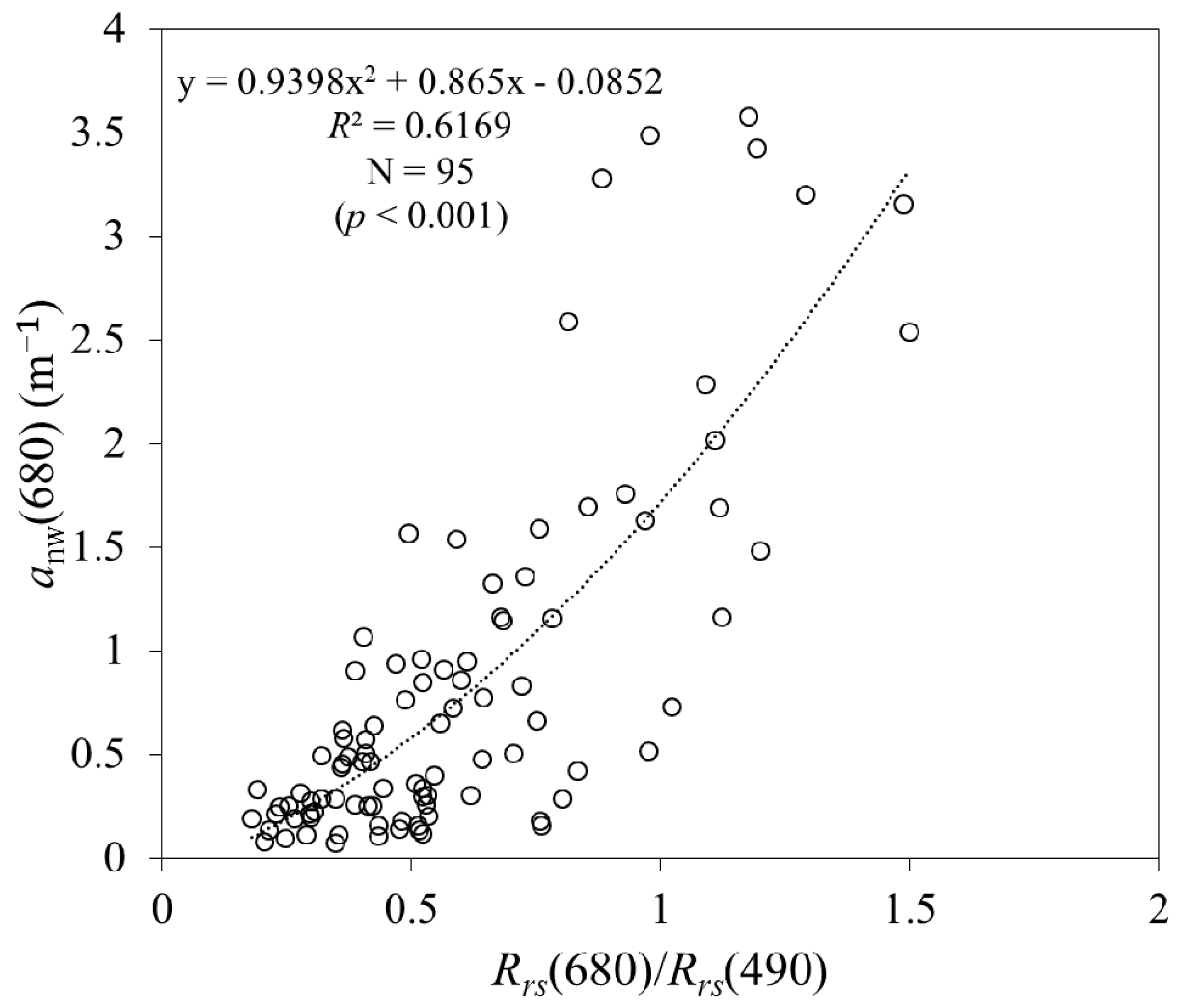
(2) Calibrating a(λ0) formula (step 2 in Table 3). a(λ) was significantly underestimated, when reference wavelength in Equation (7) was accepted as 55X or 670 nm. Through the correlation analysis, it was found that λ0 = 680 nm is the optimal reference wavelength. Based on our in situ data, the following equation relating non-water absorption at 680 nm, anw(680), with the spectral ratio Rrs(680)/Rrs(490) was derived as follows (Figure 3):
(3) Step 3 is from QAA_v6 (step 3 in Table 3).
(4) Calibrating the Y in Equation (8) (step 4 in Table 3). The unknown parameters m and n were obtained by fitting a power regression with 466 sets of individual in situ measured data including bbp(680) and its corresponding Y values derived from Equation (8). The power regression is:
where it was found that m = 1.75 and n = −0.05, with the significance level p < 0.001 (Figure 4).
(5) Step 5 is from QAA_v6 (step 5 in Table 3).
(6) Step 6 is from QAA_v6 (step 6 in Table 3).
(7) Establishing ag(λ) formula (step 7 in Table 3). Though regression analysis, Equation (11) is fitted by in situ data, where it was found that j1 = 4.802 and j2 = 0.8055, with the significance level p < 0.001 (Figure 5).
(8) Step 8 is from QAA_CDOM (step 8 in Table 3). The unknown parameters p and q were obtained by fitting a power regression with in situ measured data including spectral ratio Rrs(555)/Rrs(490) and its corresponding S values derived from Equation (10). The power regression is:
where it was found that p = 0.0112 and q = 1.0401, with the significance level p < 0.001.
3.2. In Situ Data for QAA_cj Validation
Both QAA_cj and QAA_v6 algorithms are applied separately to test an accuracy of retrieved optical parameters in the Changjiang estuarine and coastal waters. A reference wavelength λ0 = 670 nm has been selected for the Rrs(λ) dependence in Equation (7) following the QAA_v6 spectral criterion.
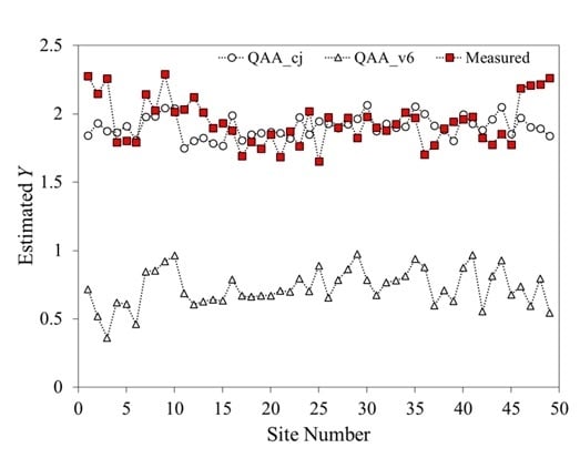
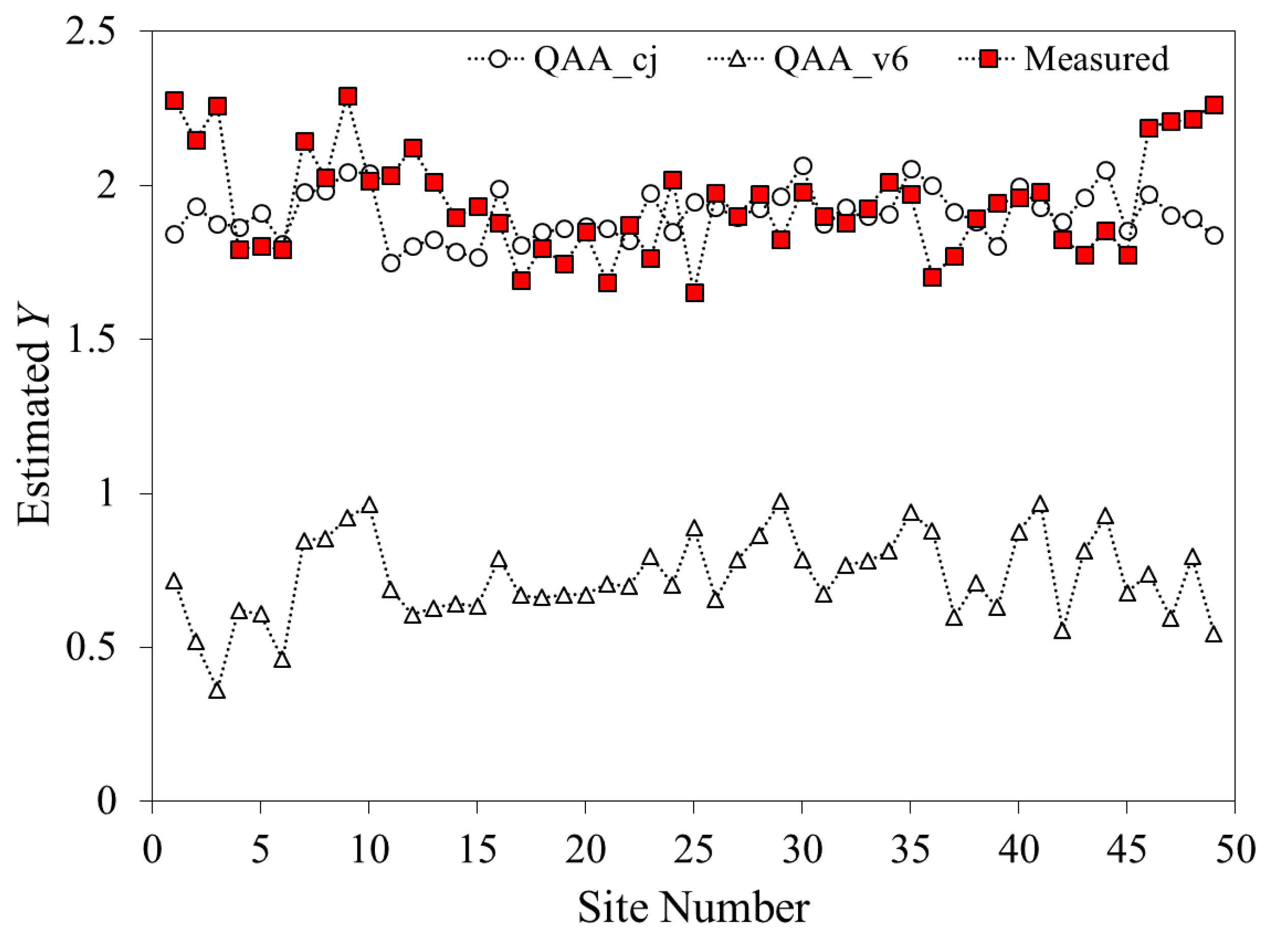
Figure 6 shows the comparison of Y values derived from in situ bbp(λ) by the QAA_v6 (triangles) and QAA_cj (circles) algorithms based on the validation database. It is clear to be seen that values of Y estimated by QAA_cj range from 1.7 to 2.3, which is much closer to the measured values, whereas, the QAA_v6 estimation is largely underestimated (0.3~1).
Figure 7 shows the comparison of in situ and retrieval results of a(λ), in which two short wavelengths (e.g., 443 or 555 nm) and two long wavelengths (e.g., 680 or 715 nm) were compared. Compared with in situ data, QAA_cj has good consistency in short wavelength and long wavelength bands; however, there is a slight overestimation in the short wavelength spectral range. In comparison, QAA_v6 has an obvious underestimation, especially in the long wavelength range. The assessment results for retrieved total absorption from 412 to 715 nm are summarized in Table 4. Statistical results show that two algorithms are similar in the short wavelength range (412, 443, 490, 555 nm), but QAA_cj is more accurate than QAA_v6 in the long wavelength domain (660, 680, 715 nm). Specifically, QAA_cj has a better accuracy in estimating a(λ) than QAA_v6 at 715 nm, for which R2 are 0.73 and 0.30, respectively. Poor RMSE and bias results are mainly caused by the bias of Y value estimation. In addition, the QAA_v6 algorithm performed better than QAA_cj at 412 and 443 nm, which could be explained by the inaccuracies caused by the empirical Equation (18).
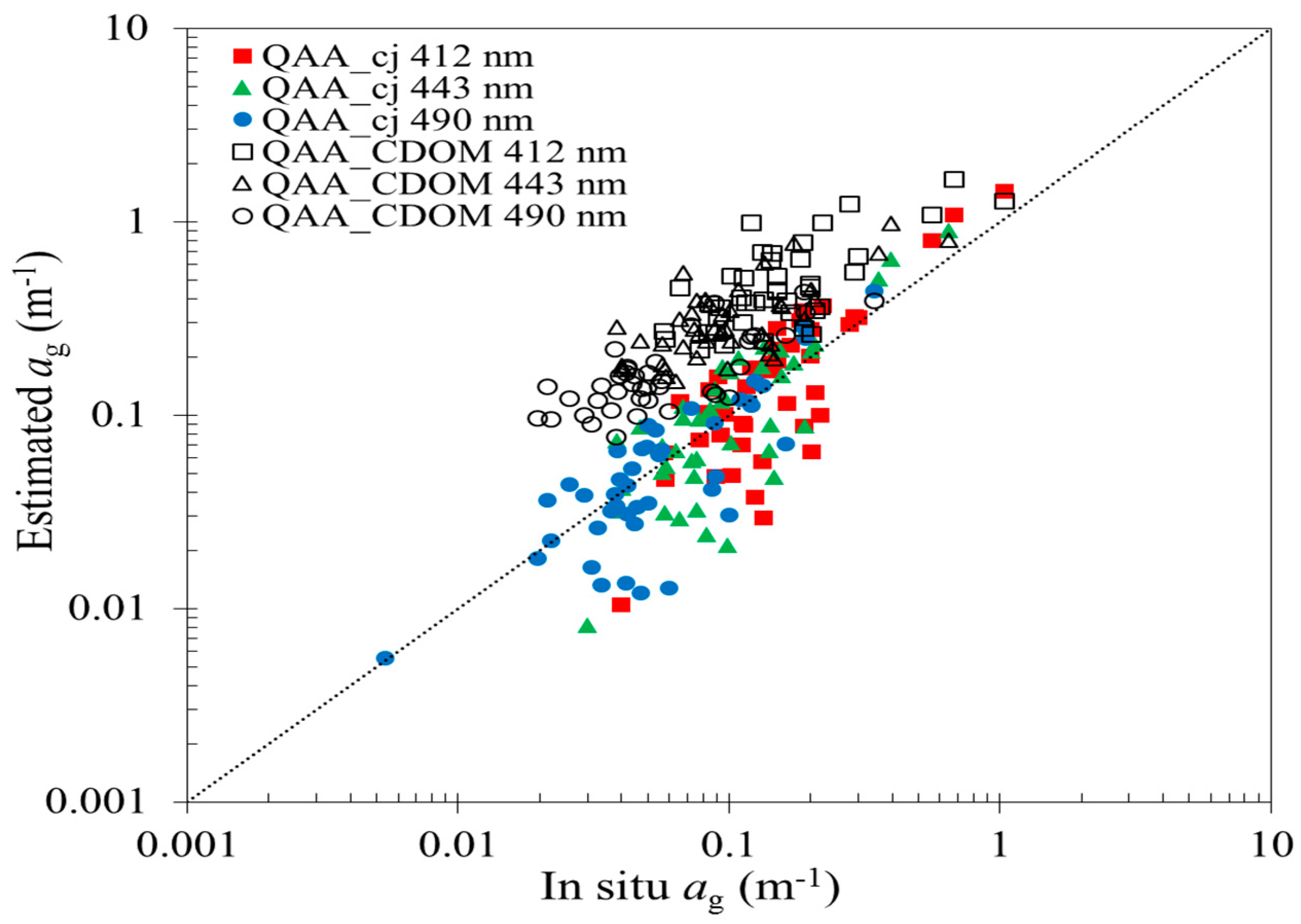
Since ag and ad have similar absorption features, ag cannot be extracted from the adg by the QAA_v6 algorithm. Therefore, QAA_cj-derived ag(λ) values were compared only with the QAA_CDOM-derived ag(λ) values (Figure 8), and the assessment results are shown in Table 5. QAA_cj has a better accuracy in estimating ag(443) with RMSE, MARE and bias of 0.07, 0.42 and 0.018 m−1 compared with those of 0.25, 2.39 and 0.22 m−1, respectively, from QAA_CDOM. The retrival accuracy of ag(λ) at wavelengths of 412 and 490 nm is improved as well (Table 5).
3.3. Satellite Data for QAA_cj Validation
QAA_cj (Table 3, steps 0 to 6) and QAA_v6 (steps 0 to 6) are applied toGOCI to validate the accuracy of a(λ) based on the in situ data (Figure 9, Table 6). When applying to GOCI, QAA_cj has a consistency with in situ data at 443, 555, 680 nm, of which R2 is larger than 0.8 at 680 nm. It shows that the QAA_cj yielded a better accuracy in estimating a(680) with RMSE and bias of −0.025 and 0.10 m−1, compared with those of 0.62 and 0.31 m−1 from QAA_v6. However, the inversion result is slightly poor at 745 nm (Figure 9, Table 6).
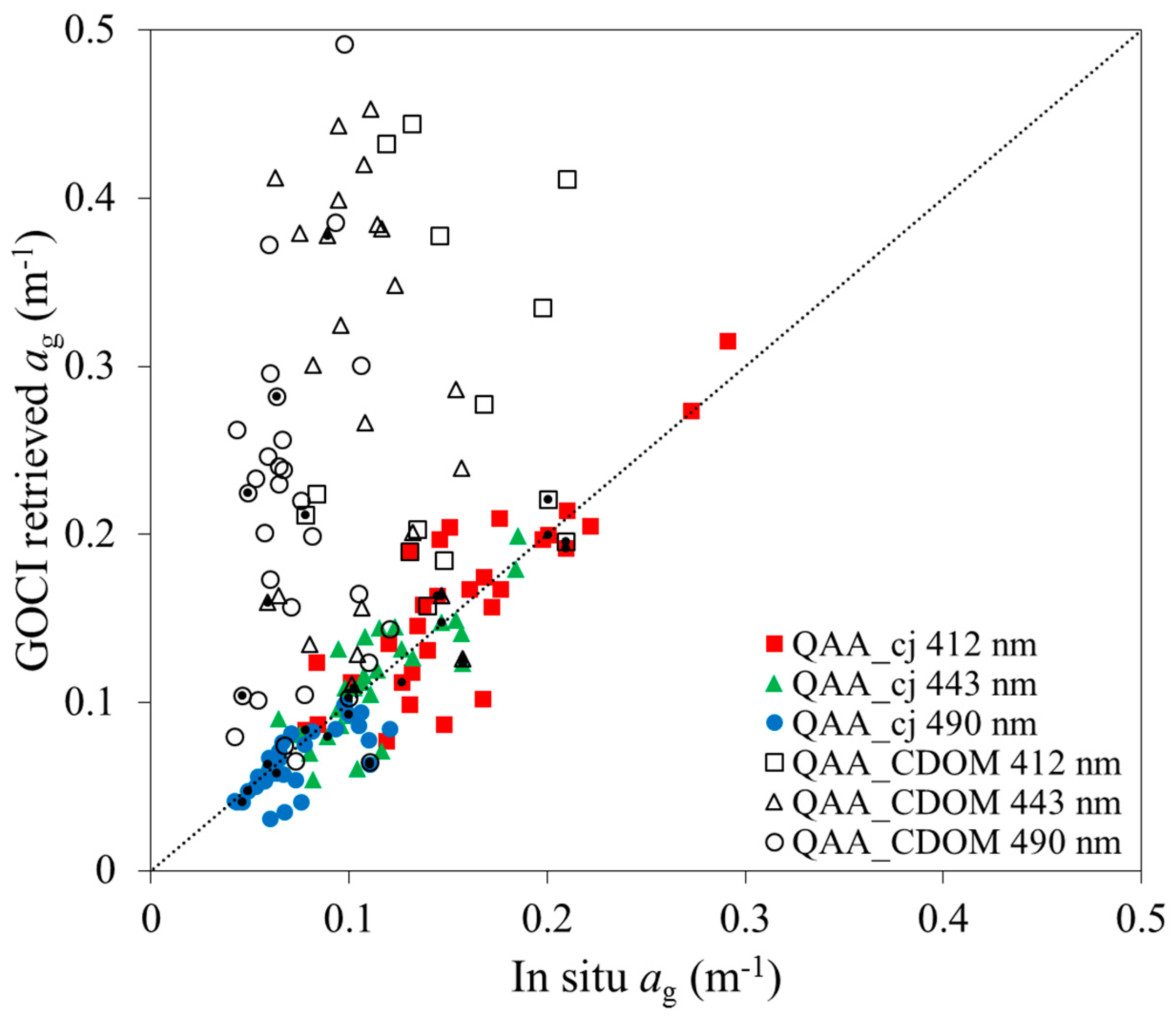
QAA_cj (Table 3, Steps 7 and 8) and QAA_CDOM algorithms are applied to GOCI to validate the accuracy of ag(λ), compared with in situ data (Figure 10). It is indicated that estimations from the QAA_CDOM have lower agreement with the in situ values. Meanwhile, QAA_cj has a better consistency in estimating ag(λ) at 412, 443 and 490 nm, compared with the QAA_CDOM. Remarkably, the retrieval accuracy is optimal at wavelength of 443 nm, at which MARE is 0.14, R2 is 0.70, whereas QAA_CDOM yields MARE = 2.34 and R2 = 0.11 (Table 7).
4. Discussion
CDOM absorption is a major variable in remote sensing algorithms for deriving concentrations of optically active components of sea water [56]. Based on the spectral absorption characteristic of CDOM, Del Castillo and Miller [14], D’Sa and Miller [18] and Ficek et al. [13] established statistical relationships between ag and Rrs ratio (using different wavelengths) in Mississippi River and the Baltic. Using Rrs(λ) to calculate a and further to separate out adg and aph, semi-analytical models, such as GSM [23] and QAA [28], were developed based on IOCCG dataset and in situ data, while Brando and Dekker [5] and Hoge and Lyon [22] developed models using in situ data in Fitzroy Estuary and U.S. Middle Atlantic Bight.
The QAA_cj algorithm was developed to give an opportunity to obtain more accurate estimates for both total and partial absorption coefficients in highly turbid waters, such as the Changjiang estuarine and coastal waters. For this purpose, we calibrated empirical parameters of the QAA_v6 and QAA_CDOM algorithms. Proofs of improvement made in these algorithms are shown in Table 4, Table 5, Table 6 and Table 7 and Figure 6, Figure 7, Figure 8, Figure 9 and Figure 10. For example, a total absorption coefficient a(λ) retrieved by QAA_v6 was underestimated in highly turbid waters, while QAA_cj-based values were closer to in situ data (Table 4, Figure 7). As for CDOM spectral absorption ag(λ), on the one hand it could not be estimated by the QAA algorithm and on the other hand it was overestimated by the QAA_CDOM algorithm (Figure 8), while the QAA_cj retrieved value of ag(443) has RMSE and R2 of 0.07 m−1 and 0.90, respectively, compared with in situ data (Table 5). Nevertheless, the accuracy of ag(λ) derived from the QAA_cj in highly turbid waters still remains to be a challenge.
We also wish to note that our findings may have great values not only for numerous scientists and for decision makers working for the East China estuarine and coastal waters, but also for many other investigators. As it has been found by Sokoletsky et al. [57], the biogeochemistry-optical relationships for the East China estuarine and coastal waters are very similar to that of the Gironde Estuary [58] and the Southern North Sea [59]. Thus, these findings really allow generalizing all conclusions of our study.
Since the aim of the study was the investigation of underwater IOPs, we used a conversion from the surface remote-sensing reflectance Rrs(λ) to its underwater analog, rrs(λ). Therefore, in this study, we used the formula proposed by Sokoletsky et al. [57] to calculate rrs(λ) from Rrs(λ). Sokoletsky and Shen [47] showed that although relations between Rrs(λ) and rrs(λ) are close for different models, the particular model parameters may play an important role in the inversion results. In addition, we have used only clear and cloudless sky conditions to measure Rrs(λ) to do calculations more simple and closer to remote-sensing results, Figure 2b.
Equation (4) is an approximation to the exact solution of the radiative transfer equation [60], which may cause a normalized (to the mean value) root-mean-square error of about 20% [61]. Moreover, it is inappropriate to regard parameters of this equation (i.e., g0 and g1) as constants. These parameters are associated with the solar zenith angle and water properties, and vary with water composition scattering properties [62]. Consequently, g0 and g1 have influence on bb(λ), when using QAA, it will further affect the inversion accuracy of a(λ). Lee et al. [62] partitioned and weighted parameter g according to the molecular (water itself) and particulate contributions to the backscattering coefficient. In this study, however, this approach was not exploited.
According to Lee et al. [63], the a(λ0) and Y have an impact on performance of the QAA. Y is a parameter which describes spectral variation of bbp(λ) [64], and the variation of Y depends on water composition and size of particles according to the Mie theory [65]. Yang et al. [38] found that Y values have a great impact on the retrieval results, particularly in the shorter spectral bands. Figure 6 shows that the QAA_v6 algorithm has a low accuracy in estimating Y, which perhaps caused by the insufficient capability of this algorithm considering the complex optical features of the Changjiang estuarine and coastal waters. The ranges of Y values derived from the QAA_cj and the QAA_v6 are from 1.5 to 2.5 and from 0.3 to 1, respectively (Figure 6). Even though our algorithm for Y (Equation 19) does not yield a reasonable correlation with the measured values (Figure 6), we have chosen to keep it for generalization purposes, and we are planning to improve the Y model in the following study.
In this study, we have changed the reference wavelength from 670 nm to 680 nm. Although it is an insignificant change of spectral, the retrieval accuracy of calibrated formula was improved effectively when applied to Changjiang estuarine and coastal waters (Table 4 and Table 5). We reproduced a(λ) and ag(λ) from the GOCI images using the QAA_v6, QAA_CDOM and QAA_cj algorithms, and presented the comparison results in Figure 9 and Figure 10. As shown in Figure 9, differences between our algorithm and in situ data is smaller than those between the QAA_v6 and in situ data for the whole blue to near infrared spectral range. Similar findings were found for the ag(λ) retrieving in the blue spectral domain (Figure 10).
Some contradicting results derived from QAA algorithm were discovered from existing literature as well. For example, investigations by Qin et al. [66] and Shanmugam et al. [67] have shown that there is a lower accuracy for retrieving absorption components in some regions of the ocean by QAA. Zheng et al. [68] have also shown that the accuracy of QAA algorithm (v5) varied greatly in deriving a(λ) (from 2% to 28%) and bb(λ) (from 8% to 14%) depending on wavelength and ocean site. In addition, Zhu et al. [69] compared and verified 15 CDOM retrieval algorithms (empirical, semi-analytical, optimization, and matrix inversion algorithms), and pointed out that the QAA_CDOM algorithm was optimal. The reason of this is that CDOM has negligible backscattering, whereas inorganic particles have strong backscattering, even in longer wavelength [27]. Several researches find that QAA_CDOM has a good accuracy in obtaining the ap(λ) from bbp(λ) [26,27,69]. However, QAA_CDOM has some empirical parameters, which are required to be calibrated according to specific study area. Figure 10 shows that after calibration, ag(λ) has a significant improvement at 412, 443, 490 nm. It seems obvious that better accuracy in ag(λ) leads to improvement of a retrieval accuracy for aph and ad.
5. Conclusions
Through calibration and validation, we improved empirical parameters of QAA_v6 and QAA_CDOM IOPs algorithms, and thus developed a new algorithm, namely, QAA_cj, which is suitable for the highly turbid Changjiang estuary and adjacent areas. Results of validation prove that QAA_cj has a better accuracy in retrieving a(λ) and ag(λ), compared with the QAA_v6 and QAA_CDOM. a(λ) derived from QAA_cj is in a good agreement with in situ and GOCI data, where RMSE ranges from 0.35 to 1.17 m−1, MARE from 0.11 to 0.52, bias from −1.23 to 0.66 m−1 and R2 is from 0.28 to 0.82. As for ag(λ), RMSE ranges from 0.035 to 0.12 m−1, MARE from 0.14 to 0.42, bias from −0.0086 to 0.033 m−1 and R2 is from 0.53 to 0.92.
The improvement of a(λ) and ag(λ) retrieval accuracy will help to provide theoretical basis for the release of satellite product and further study on optical properties. Reliable CDOM products can provide information on the internal movements and nutrients structure of Changjiang diluted water and mechanisms of hydrodynamics in the Changjiang estuarine and coastal waters. The trace of CDOM can advance our understanding of the land-ocean interaction processes through monitoring spatial-temporal distribution of the river plume into sea. In the future, we will focus on exploring the relationships between environmental factors and optical parameters, in combination with satellite data and physical models.
Acknowledgments
Massive field cruise campaigns were funded by the National Natural Science Foundation of China (NSFC) joint cruise programmes. This study is supported by the NSFC projects (no. 41771378 and no. 41271375), Ministry of Science and Technology of China (no. 2016YFE0103200) and the research foundation of SKLEC (Grant no. 2015KYYW04). The authors would like to thank the crew members of the “Runjiang” ship and all young scientists participating in the collection of samples. We also thank the KORDI/KOSC for providing GOCI data. We acknowledge contributors to data accumulation and data processing including Xiaodao Wei, Pei Shang and Yanqun Pan. The insightful and constructive comments from the editor and three anonymous reviewers are also greatly appreciated.
Author Contributions
Yongchao Wang and Fang Shen conceived and designed the study. Fang Shen provided part of the in situ data. Yongchao Wang wrote the programs and performed the experiments, the results were examined by Fang Shen. All authors contributed to the writing and approved the final manuscript.
Conflicts of Interest
The authors declare no conflict of interest.
References
- Mobley, C.D. Light and Water: Radiative Transfer in Natural Waters; Academic Press: Cambridge, MA, USA, 1994. [Google Scholar]
- Lee, Z.P.; Carder, K.L.; Peacock, T.G.; Davis, C.O.; Mueller, J.L. Method to derive ocean absorption coefficients from remote-sensing reflectance. Appl. Opt. 1996, 35, 453–462. [Google Scholar] [CrossRef] [PubMed]
- Stramski, D.; Boss, E.; Bogucki, D.; Voss, K.J. The role of seawater constituents in light backscattering in the ocean. Prog. Oceanogr. 2004, 61, 27–56. [Google Scholar] [CrossRef]
- Le, C.F.; Li, Y.M.; Zha, Y.; Sun, D.; Yin, B. Validation of a quasi-analytical algorithm for highly turbid eutrophic water of Meiliang Bay in Taihu Lake, China. IEEE Trans. Geosci. Remote Sens. 2009, 47, 2492–2500. [Google Scholar]
- Brando, V.E.; Dekker, A.G. Satellite hyperspectral remote sensing for estimating estuarine and coastal water quality. IEEE Trans. Geosci. Remote Sens. 2003, 41, 1378–1387. [Google Scholar] [CrossRef]
- Giardino, C.; Brando, V.E.; Dekker, A.G.; Strömbeck, N.; Candiani, G. Assessment of water quality in Lake Garda (Italy) using Hyperion. Remote Sens. Environ. 2007, 109, 183–195. [Google Scholar] [CrossRef]
- Yang, W.; Matsushita, B.; Chen, J.; Fukushima, T. A relaxed matrix inversion method for retrieving water constituent concentrations in case II waters: The case of Lake Kasumigaura, Japan. IEEE Trans. Geosci. Remote Sens. 2011, 49, 3381–3392. [Google Scholar] [CrossRef] [Green Version]
- Bricaud, A.; Morel, A.; Prieur, L. Absorption by dissolved organic matter of the sea (yellow substance) in the UV and visible domains. Limnol. Oceanogr. 1981, 26, 43–53. [Google Scholar] [CrossRef]
- Nieke, B.; Reuter, R.; Heuermann, R.; Wang, H.; Babin, M.; Therriault, J.C. Light absorption and fluorescence properties of chromophoric dissolved organic matter (CDOM), in the St. Lawrence Estuary (Case 2 waters). Cont. Shelf Res. 1997, 17, 235–252. [Google Scholar] [CrossRef]
- Darecki, M.; Weeks, A.; Sagan, S.; Kowalczuk, P.; Kaczmarek, S. Optical characteristics of two contrasting Case 2 waters and their influence on remote sensing algorithms. Cont. Shelf Res. 2003, 23, 237–250. [Google Scholar] [CrossRef]
- Hu, C.; Muller-Karger, F.E.; Taylor, C.J.; Carder, K.L.; Kelble, C.; Johns, E.; Heil, C.A. Red tide detection and tracing using MODIS fluorescence data: A regional example in SW Florida coastal waters. Remote Sens. Environ. 2005, 97, 311–321. [Google Scholar] [CrossRef]
- Bowers, D.G.; Brett, H.L. The relationship between CDOM and salinity in estuaries: An analytical and graphical solution. J. Mar. Syst. 2008, 73, 1–7. [Google Scholar] [CrossRef]
- Ficek, D.; Zapadka, T.; Dera, J. Remote sensing reflectance of Pomeranian lakes and the Baltic. Oceanologia 2011, 53, 959–970. [Google Scholar] [CrossRef]
- Del Castillo, C.E.; Miller, R.L. On the use of ocean color remote sensing to measure the transport of dissolved organic carbon by the Mississippi River Plume. Remote Sens. Environ. 2008, 112, 836–844. [Google Scholar] [CrossRef]
- Griffin, C.G.; Frey, K.E.; Rogan, J.; Holmes, R.M. Spatial and interannual variability of dissolved organic matter in the Kolyma River, East Siberia, observed using satellite imagery. J. Geophys. Res. Biogeosci. 2011, 116. [Google Scholar] [CrossRef]
- Kutser, T.; Pierson, D.C.; Tranvik, L.; Reinart, A.; Sobek, S.; Kallio, K. Using satellite remote sensing to estimate the colored dissolved organic matter absorption coefficient in lakes. Ecosystems 2005, 8, 709–720. [Google Scholar] [CrossRef]
- Mannino, A.; Russ, M.E.; Hooker, S.B. Algorithm development and validation for satellite-derived distributions of DOC and CDOM in the US Middle Atlantic Bight. J. Geophys. Res. Oceans 2008, 113. [Google Scholar] [CrossRef]
- D’Sa, E.J.; Miller, R.L. Bio-optical properties in waters influenced by the Mississippi River during low flow conditions. Remote Sens. Environ. 2003, 84, 538–549. [Google Scholar] [CrossRef]
- Carder, K.L.; Chen, F.R.; Lee, Z.P.; Hawes, S.K.; Kamykowski, D. Semianalytic Moderate-Resolution Imaging Spectrometer algorithms for chlorophyll a and absorption with bio-optical domains based on nitrate-depletion temperatures. J. Geophys. Res. Oceans 1999, 104, 5403–5421. [Google Scholar] [CrossRef]
- Wang, P.; Boss, E.S.; Roesler, C. Uncertainties of inherent optical properties obtained from semianalytical inversions of ocean color. Appl. Opt. 2005, 44, 4074–4085. [Google Scholar] [CrossRef] [PubMed]
- Babin, M.; Stramski, D.; Ferrari, G.M.; Claustre, H.; Bricaud, A.; Obolensky, G.; Hoepffner, N. Variations in the light absorption coefficients of phytoplankton, nonalgal particles, and dissolved organic matter in coastal waters around Europe. J. Geophys. Res. Oceans 2003, 108. [Google Scholar] [CrossRef]
- Hoge, F.E.; Lyon, P.E. Satellite retrieval of inherent optical properties by linear matrix inversion of oceanic radiance models: An analysis of model and radiance measurement errors. J. Geophys. Res. Oceans 1996, 101, 16631–16648. [Google Scholar] [CrossRef]
- Maritorena, S.; Siegel, D.A.; Peterson, A.R. Optimization of a semianalytical ocean color model for global-scale applications. Appl. Opt. 2002, 41, 2705–2714. [Google Scholar] [CrossRef] [PubMed]
- Roesler, C.S.; Perry, M.J. In situ phytoplankton absorption, fluorescence emission, and particulate backscattering spectra determined from reflectance. J. Geophys. Res. Oceans 1995, 100, 13279–13294. [Google Scholar] [CrossRef]
- Lee, Z.; Weidemann, A.; Kindle, J.; Arnone, R.; Carder, K.L.; Davis, C. Euphotic zone depth: Its derivation and implication to ocean-color remote sensing. J. Geophys. Res. Oceans 2007, 112. [Google Scholar] [CrossRef]
- Zhu, W.; Yu, Q. Inversion of Chromophoric Dissolved Organic Matter from EO-1 Hyperion Imagery for Turbid Estuarine and Coastal Waters. Geosci. Remote Sens. IEEE Trans. 2013, 51, 3286–3298. [Google Scholar] [CrossRef]
- Zhu, W.; Yu, Q.; Tian, Y.Q.; Chen, R.F.; Gardner, G.B. Estimation of chromophoric dissolved organic matter in the Mississippi and Atchafalaya river plume regions using above-surface hyperspectral remote sensing. J. Geophys. Res. Oceans 2011, 116. [Google Scholar] [CrossRef]
- Lee, Z.; Carder, K.L.; Arnone, R.A. Deriving inherent optical properties from water color: A multiband quasi-analytical algorithm for optically deep waters. Appl. Opt. 2002, 41, 5755–5772. [Google Scholar] [CrossRef] [PubMed]
- Lee, Z. Diffuse attenuation coefficient of downwelling irradiance: An evaluation of remote sensing methods. J. Geophys. Res. 2005, 110. [Google Scholar] [CrossRef]
- Lee, Z. Remote Sensing of Inherent Optical Properties: Fundamentals, Tests of Algorithms, and Applications. In Reports of the International Ocean-Colour Coordinating Group; Lee, Z.-P., Ed.; IOCCG: Dartmouth, NS, Canada, 2006. [Google Scholar]
- Lee, Z. Update of the Quasi-Analytical Algorithm (QAA_v6). 2014. Available online: http://www.ioccg.org/groups/Software_OCA/QAA_v6_2014209.pdf (accessed on 19 November 2017).
- Lee, Z.; Carder, K.L. Absorption spectrum of phytoplankton pigments derived from hyperspectral remote-sensing reflectance. Remote Sens. Environ. 2004, 89, 361–368. [Google Scholar] [CrossRef]
- Lee, Z.; Shang, S.; Hu, C.; Lewis, M.; Arnone, R.; Li, Y.; Lubac, B. Time series of bio-optical properties in a subtropical gyre: Implications for the evaluation of interannual trends of biogeochemical properties. J. Geophys. Res. Oceans 2010, 115. [Google Scholar] [CrossRef]
- Lee, Z.; Lance, V.P.; Shang, S.; Vaillancourt, R.; Freeman, S.; Lubac, B.; Hargreaves, B.R.; del Castillo, C.; Miller, R.; Twardowski, M. An assessment of optical properties and primary production derived from remote sensing in the Southern Ocean (SO GasEx). J. Geophys. Res. Oceans 2011, 116. [Google Scholar] [CrossRef]
- Shang, S.; Lee, Z.; Wei, G. Characterization of MODIS-derived euphotic zone depth: Results for the China Sea. Remote Sens. Environ. 2011, 115, 180–186. [Google Scholar] [CrossRef]
- Wang, W.; Dong, Q.; Shang, S.; Wu, J.; Lee, Z. An evaluation of two semi-analytical ocean color algorithms for waters of the South China Sea. J. Trop. Oceanogr. 2009, 28, 35–42. [Google Scholar]
- Li, S.; Song, K.; Mu, G.; Zhao, Y.; Ma, J.; Ren, J. Evaluation of the Quasi-Analytical Algorithm (QAA) for Estimating Total Absorption Coefficient of Turbid Inland Waters in Northeast China. IEEE J. Sel. Top. Appl. Earth Obs. Remote Sens. 2016, 9, 4022–4036. [Google Scholar] [CrossRef]
- Yang, W.; Matsushita, B.; Chen, J.; Yoshimura, K.; Fukushima, T. Retrieval of Inherent Optical Properties for Turbid Inland Waters From Remote-Sensing Reflectance. IEEE Trans. Geosci. Remote Sens. 2013, 51, 3761–3773. [Google Scholar] [CrossRef]
- Yu, X.; Shen, F.; Liu, Y. Light absorption properties of CDOM in the Changjiang (Yangtze) estuarine and coastal waters: An alternative approach for DOC estimation. Estuar. Coast. Shelf Sci. 2016, 181, 302–311. [Google Scholar] [CrossRef]
- Shen, F.; Zhou, Y.; Hong, G. Absorption Property of Non-algal Particles and Contribution to Total Light Absorption in Optically Complex Waters, a Case Study in Yangtze Estuary and Adjacent Coast. In Advances in Computational Environment Science; Springer: Berlin/Heidelberg, Germany, 2012; pp. 61–66. [Google Scholar]
- Shen, F.; Salama, M.S.; Zhou, Y.; Li, J.; Su, Z.; Kuang, D. Remote-sensing reflectance characteristics of highly turbid estuarine waters—A comparative experiment of the Yangtze River and the Yellow River. Int. J. Remote Sens. 2010, 31, 2639–2654. [Google Scholar] [CrossRef]
- Yuan, R.; Wu, H.; Zhu, J.; Li, L. The response time of the Changjiang plume to river discharge in summer. J. Mar. Syst. 2016, 154, 82–92. [Google Scholar] [CrossRef]
- Wu, H.; Shen, J.; Zhu, J.; Zhang, J.; Li, L. Characteristics of the Changjiang plume and its extension along the Jiangsu Coast. Cont. Shelf Res. 2014, 76, 108–123. [Google Scholar] [CrossRef]
- Chang, P.H.; Isobe, A. A numerical study on the Changjiang diluted water in the Yellow and East China Seas. J. Geophys. Res. Oceans 2003, 108. [Google Scholar] [CrossRef]
- Zhu, J.; Ding, P.; Hu, D. Observation of the diluted water and plume front off the changjiang river estuary during august 2000. Oceanol. Limnol. Sin. 2003, 34, 249–255. [Google Scholar]
- Mobley, C.D. Estimation of the remote-sensing reflectance from above-surface measurements. Appl. Opt. 1999, 38, 7442–7455. [Google Scholar] [CrossRef] [PubMed]
- Sokoletsky, L.G.; Shen, F. Optical closure for remote-sensing reflectance based on accurate radiative transfer approximations: The case of the Changjiang (Yangtze) River Estuary and its adjacent coastal area, China. Int. J. Remote Sens. 2014, 35, 4193–4224. [Google Scholar] [CrossRef]
- Moore, C.; Barnard, A.; Hankins, D. Scattering Meter (BB9) User’s Guide, Revision A; WET Labs Inc.: Philomath, OR, USA, 2005; pp. 2–13. [Google Scholar]
- Pegau, W.S.; Gray, D.; Zaneveld, J.R.V. Absorption and attenuation of visible and near-infrared light in water: Dependence on temperature and salinity. Appl. Opt. 1997, 36, 6035–6046. [Google Scholar] [CrossRef] [PubMed]
- Choi, J.K.; Park, Y.J.; Ahn, J.H.; Lim, H.S.; Eom, J.; Ryu, J.H. GOCI, the world’s first geostationary ocean color observation satellite, for the monitoring of temporal variability in coastal water turbidity. J. Geophys. Res. Oceans 2012, 117. [Google Scholar] [CrossRef]
- Pan, Y.; Shen, F.; Verhoef, W. An improved spectral optimization algorithm for atmospheric correction over turbid coastal waters: A case study from the Changjiang (Yangtze) estuary and the adjacent coast. Remote Sens. Environ. 2017, 191, 197–214. [Google Scholar] [CrossRef]
- Gordon, H.R.; Brown, O.B.; Evans, R.H.; Brown, J.W.; Smith, R.C.; Baker, K.S.; Clark, D.K. A semianalytic radiance model of ocean color. J. Geophys. Res. Atmos. 1988, 93, 10909–10924. [Google Scholar] [CrossRef]
- Yang, X.; Sokoletsky, L.; Wei, X.; Shen, F. Suspended sediment concentration mapping based on the MODIS satellite imagery in the East China inland, estuarine, and coastal waters. Chin. J. Oceanol. Limnol. 2017, 35, 39–60. [Google Scholar] [CrossRef]
- Højerslev, N.K. Analytic remote-sensing optical algorithms requiring simple and practical field parameter inputs. Appl. Opt. 2001, 40, 4870–4874. [Google Scholar] [CrossRef] [PubMed]
- Aas, E. Estimates of radiance reflected towards the zenith at the surface of the sea. Ocean Sci. 2010, 6, 861. [Google Scholar] [CrossRef] [Green Version]
- Kowalczuk, P.; Olszewski, J.; Darecki, M.; Kaczmarek, S. Empirical relationships between coloured dissolved organic matter (CDOM) absorption and apparent optical properties in Baltic Sea waters. Int. J. Remote Sens. 2005, 26, 345–370. [Google Scholar] [CrossRef]
- Sokoletsky, L.; Fang, S.; Yang, X.; Wei, X. Evaluation of empirical and semianalytical spectral reflectance models for surface suspended sediment concentration in the highly variable estuarine and coastal waters of East China. IEEE J. Sel. Top. Appl. Earth Obs. Remote Sens. 2016, 9, 5182–5192. [Google Scholar] [CrossRef]
- Doxaran, D.; Froidefond, J.M.; Castaing, P. A reflectance band ratio used to estimate suspended matter concentrations in sediment-dominated coastal waters. Int. J. Remote Sens. 2002, 23, 5079–5085. [Google Scholar] [CrossRef]
- Nechad, B.; Ruddick, K.G.; Park, Y. Calibration and validation of a generic multisensor algorithm for mapping of total suspended matter in turbid waters. Remote Sens. Environ. 2010, 114, 854–866. [Google Scholar] [CrossRef]
- Lee, Z.; Ahn, Y.; Mobley, C.; Arnone, R. Removal of surface-reflected light for the measurement of remote-sensing reflectance from an above-surface platform. Opt. Express 2010, 18, 26313–26324. [Google Scholar] [CrossRef] [PubMed]
- Sokoletsky, L.G.; Lunetta, R.S.; Wetz, M.S.; Paerl, H.W. Assessment of the water quality components in turbid estuarine waters based on radiative transfer approximations. Isr. J. Plant Sci. 2012, 60, 209–229. [Google Scholar] [CrossRef]
- Lee, Z.; Carder, K.L.; Du, K. Effects of molecular and particle scatterings on the model parameter for remote-sensing reflectance. Appl. Opt. 2004, 43, 4957–4964. [Google Scholar] [CrossRef] [PubMed]
- Lee, Z.; Arnone, R.; Hu, C.; Werdell, P.J.; Lubac, B. Uncertainties of optical parameters and their propagations in an analytical ocean color inversion algorithm. Appl. Opt. 2010, 49, 369–381. [Google Scholar] [CrossRef] [PubMed]
- Gordon, H.R.; Morel, A.Y. Remote Assessment of Ocean Color for Interpretation of Satellite Visible Imagery: A Review; Springer Science & Business Media: New York, NY, USA, 1983; p. 114. [Google Scholar]
- Aurin, D.A.; Dierssen, H.M. Advantages and limitations of ocean color remote sensing in CDOM-dominated, mineral-rich coastal and estuarine waters. Remote Sens. Environ. 2012, 125, 181–197. [Google Scholar] [CrossRef]
- Qin, Y.; Brando, V.E.; Dekker, A.G.; Patissier, D.B. Validity of SeaDAS water constituents retrieval algorithms in Australian tropical coastal waters. Geophys. Res. Lett. 2007, 34. [Google Scholar] [CrossRef]
- Shanmugam, P.; Ahn, Y.; Ryu, J.; Sundarabalan, B. An evaluation of inversion models for retrieval of inherent optical properties from ocean color in coastal and open sea waters around Korea. J. Oceanogr. 2010, 66, 815–830. [Google Scholar] [CrossRef]
- Zheng, G.; Stramski, D.; Reynolds, R.A. Evaluation of the Quasi-Analytical Algorithm for estimating the inherent optical properties of seawater from ocean color: Comparison of Arctic and lower-latitude waters. Remote Sens. Environ. 2014, 155, 194–209. [Google Scholar] [CrossRef]
- Zhu, W.; Yu, Q.; Tian, Y.Q.; Becker, B.L.; Zheng, T.; Carrick, H.J. An assessment of remote sensing algorithms for colored dissolved organic matter in complex freshwater environments. Remote Sens. Environ. 2014, 140, 766–778. [Google Scholar] [CrossRef]
Figure 1.
Location of sampling stations in the Changjiang estuarine and coastal waters. (a) Samples were collected from 9 cruises in summer (May, July 2011, August 2013 and July 2015) and winter (February, March 2012, March 2013, February 2014 and March 2015); (b) Matchup stations selected for in situ and GOCI images (empty circles and stars represent the matchup time windows within ±24 h, filled circles and stars within ±3 h).
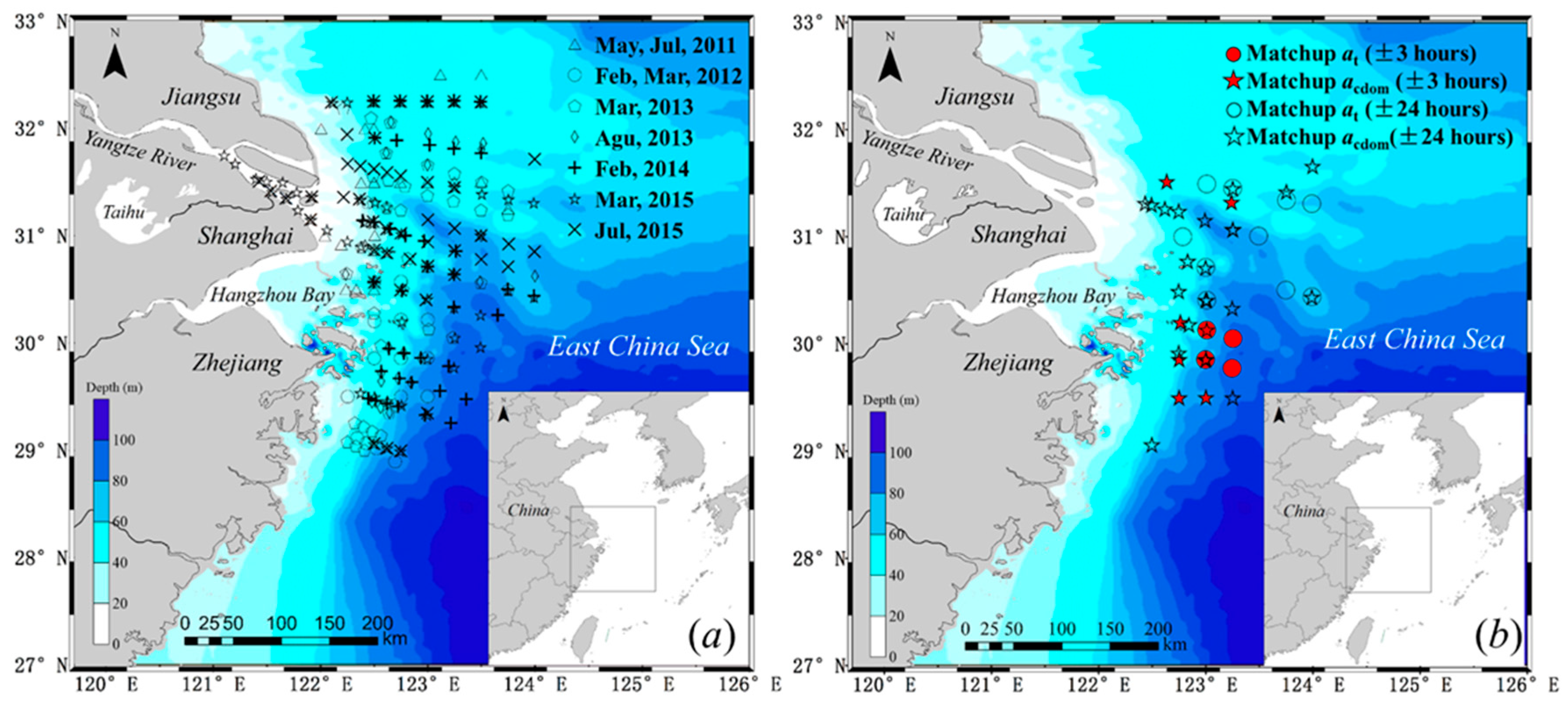
Figure 2.
(a) Typical spectra of remote-sensing reflectance collected in the Changjiang estuarine and its adjacent coastal waters; (b) The sun zenith angle and weather conditions of in situ Rrs(λ) validation data.
Figure 2.
(a) Typical spectra of remote-sensing reflectance collected in the Changjiang estuarine and its adjacent coastal waters; (b) The sun zenith angle and weather conditions of in situ Rrs(λ) validation data.
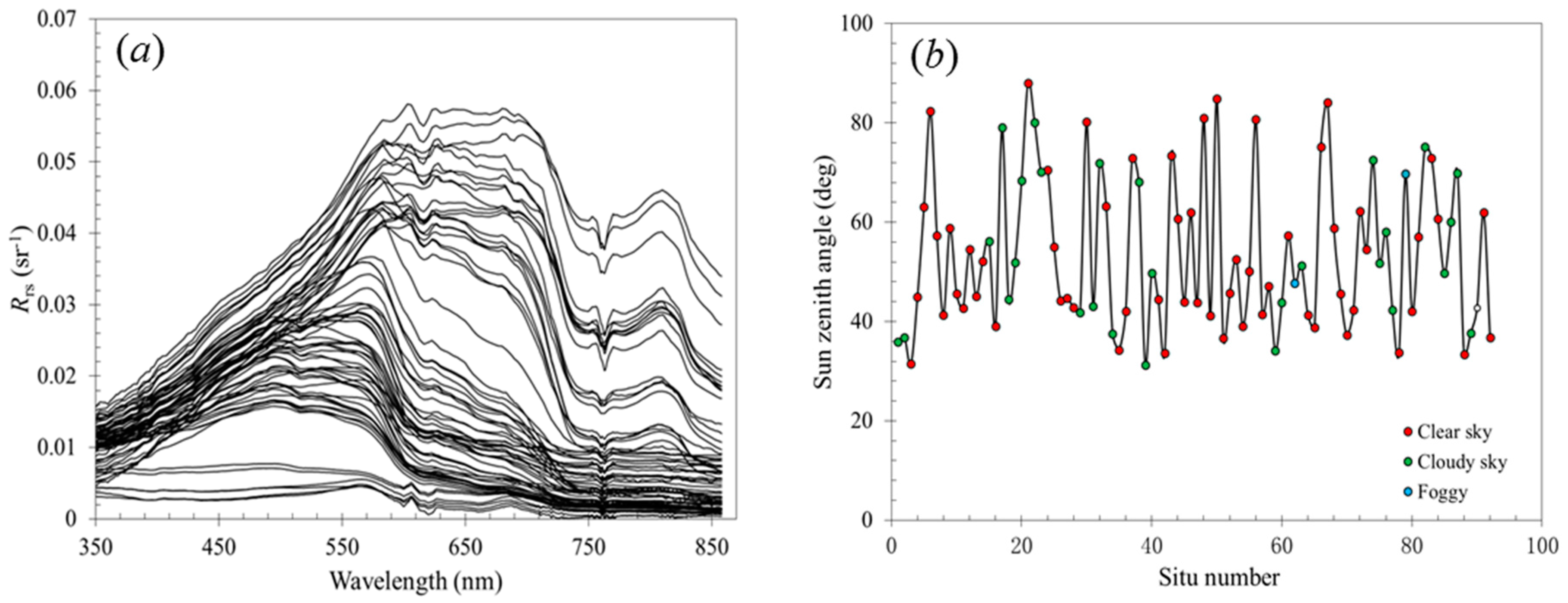
Figure 3.
Scatter plot of in situ measured anw(680) values versus Rrs(680)/Rrs(490) spectral ratios.
Figure 3.
Scatter plot of in situ measured anw(680) values versus Rrs(680)/Rrs(490) spectral ratios.

Figure 4.
Scatter plot of the Y versus bbp(680) in situ values.
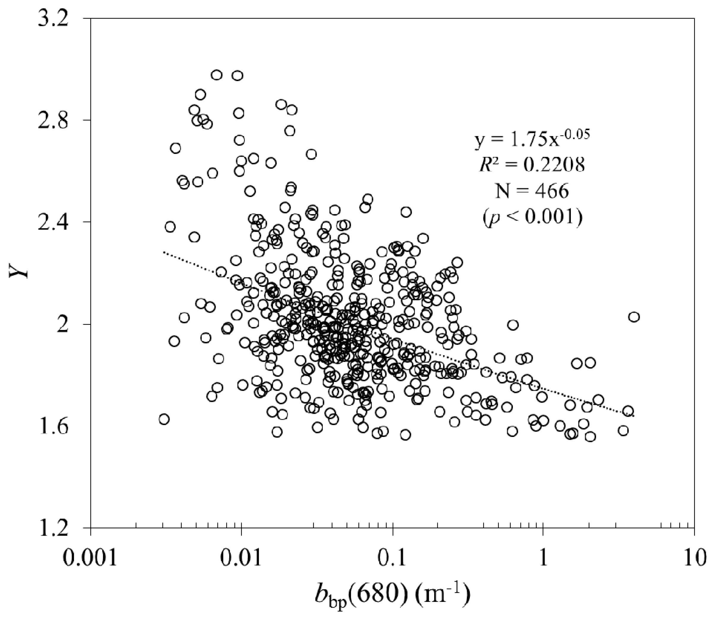
Figure 5.
Scatter plot of in situ ap(443) values plotted versus bbp(680) values.
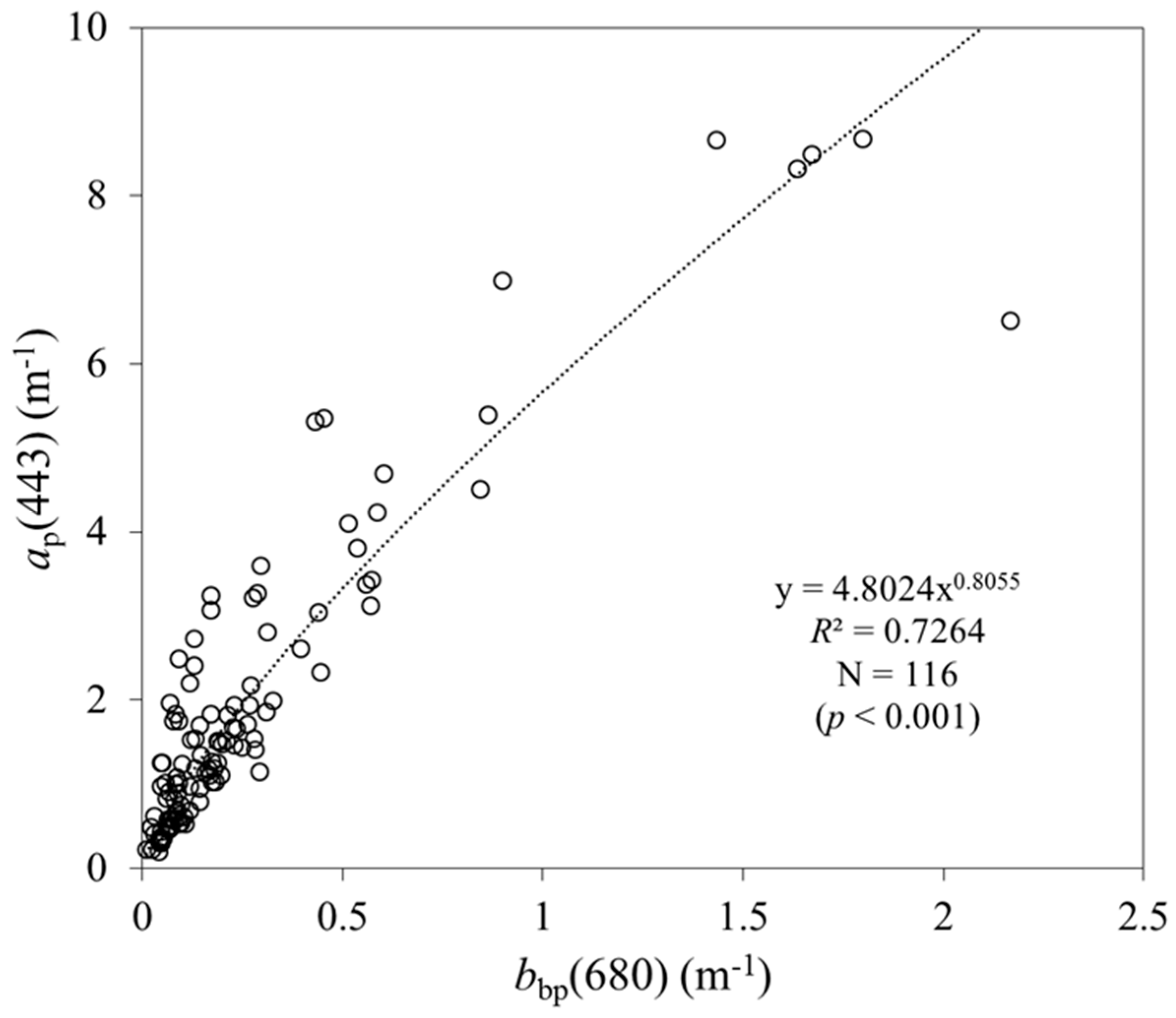
Figure 6.
Comparison of in situ and predicted Y values. The filled squares are in situ Y values, empty circles and triangles denote Y values derived from QAA_cj and QAA_v6, respectively.
Figure 6.
Comparison of in situ and predicted Y values. The filled squares are in situ Y values, empty circles and triangles denote Y values derived from QAA_cj and QAA_v6, respectively.

Figure 7.
Comparison of in situ and predicted a(λ) at 443, 555, 680 and 715 nm based on an in situ data set collected from the Changjiang estuarine and coastal waters. The filled circles and empty symbols denote retrievals from algorithms QAA_cj and QAA_v6, respectively.
Figure 7.
Comparison of in situ and predicted a(λ) at 443, 555, 680 and 715 nm based on an in situ data set collected from the Changjiang estuarine and coastal waters. The filled circles and empty symbols denote retrievals from algorithms QAA_cj and QAA_v6, respectively.
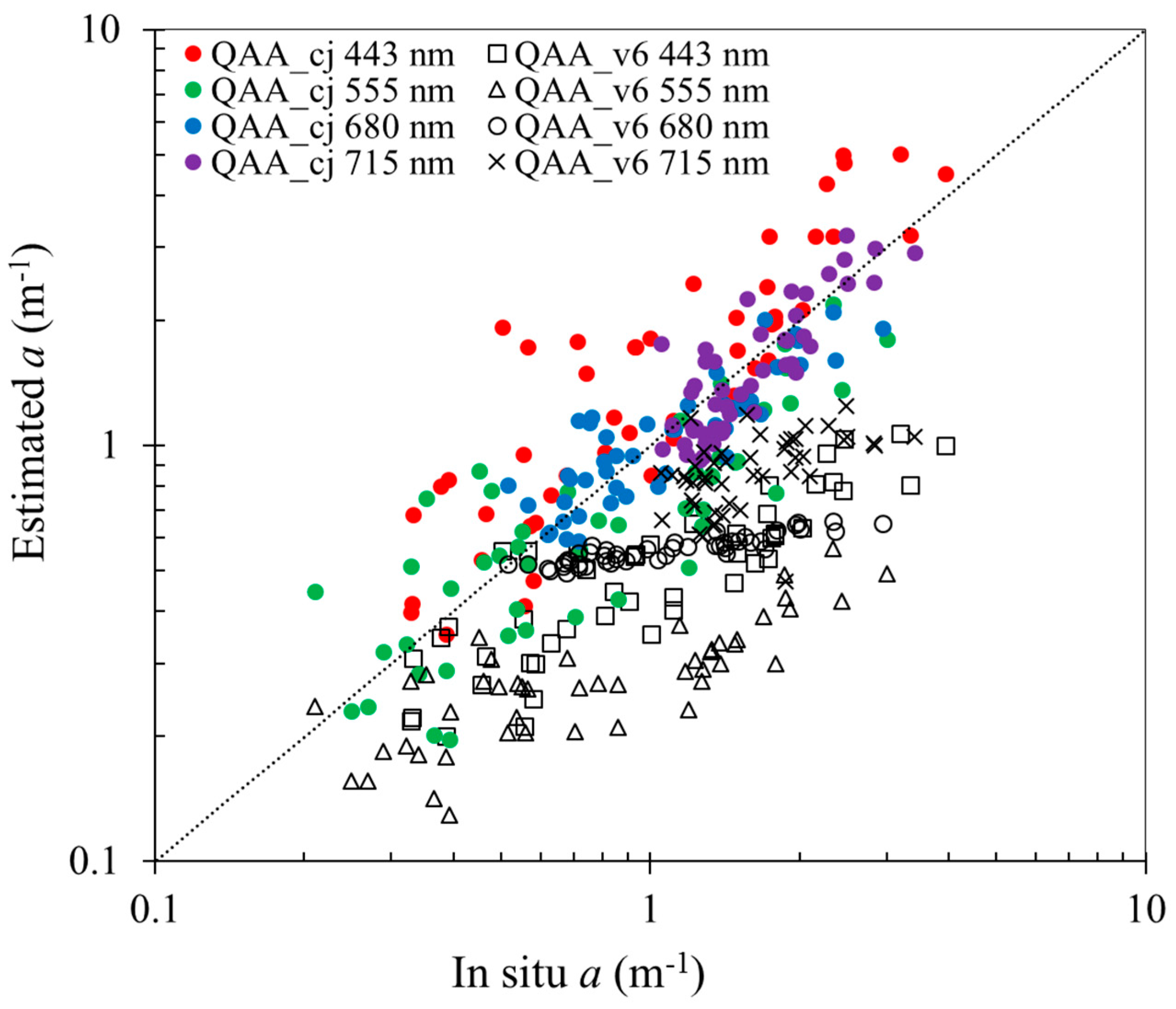
Figure 8.
Comparison of in situ and predicted ag(λ) based on an in situ data set collected from the Changjiang estuarine and its adjacent coastal waters. The filled and empty symbols denote retrievals following QAA_cj and QAA_CDOM algorithms, respectively.
Figure 8.
Comparison of in situ and predicted ag(λ) based on an in situ data set collected from the Changjiang estuarine and its adjacent coastal waters. The filled and empty symbols denote retrievals following QAA_cj and QAA_CDOM algorithms, respectively.

Figure 9.
A scattering plot of GOCI retrieved a(λ) vs. in situ a(λ) data with using the QAA_cj algorithm (filled symbols) and QAA_v6 algorithm (open symbols) at wavelengths of 443, 555, 680, and 745 nm. The symbol with a filled dot inside represents the match point within the time window of ±3 h.
Figure 9.
A scattering plot of GOCI retrieved a(λ) vs. in situ a(λ) data with using the QAA_cj algorithm (filled symbols) and QAA_v6 algorithm (open symbols) at wavelengths of 443, 555, 680, and 745 nm. The symbol with a filled dot inside represents the match point within the time window of ±3 h.
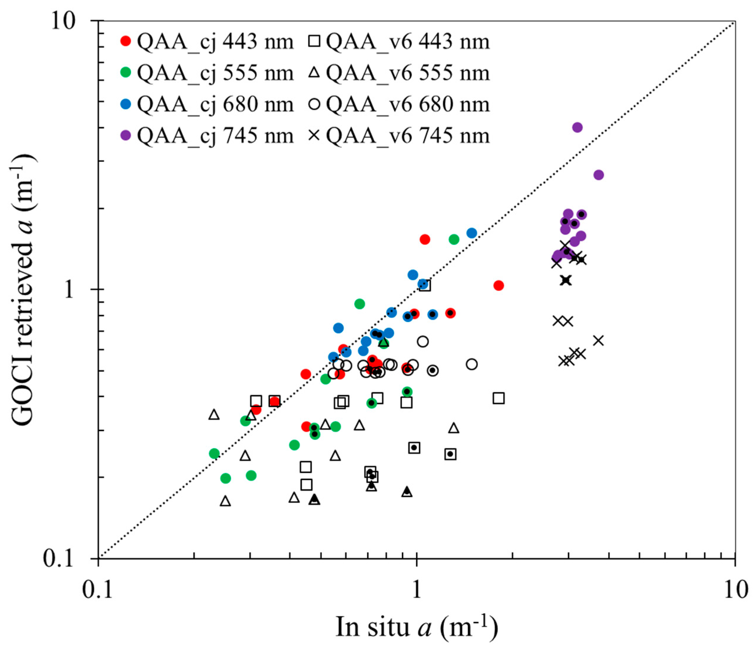
Figure 10.
A scattering plot of GOCI retrieved ag(λ) vs. in situ ag(λ) data with using the QAA_cj algorithm (filled symbols) and QAA_CDOM algorithm (open symbols) at wavelengths of 412, 443, and 490 nm. The symbol with a filled dot inside represents the match point within the time window of ±3 h.
Figure 10.
A scattering plot of GOCI retrieved ag(λ) vs. in situ ag(λ) data with using the QAA_cj algorithm (filled symbols) and QAA_CDOM algorithm (open symbols) at wavelengths of 412, 443, and 490 nm. The symbol with a filled dot inside represents the match point within the time window of ±3 h.

Table 1.
Symbols and definitions.
| Symbol | Description | Unit |
|---|---|---|
| a | Total absorption coefficient, aw + aph + ag + ad | m−1 |
| anw | Non-water absorption coefficient, a − aw = aph + ag + ad | m−1 |
| aw | Pure water absorption coefficients | m−1 |
| aph | Phytoplankton absorption coefficients | m−1 |
| ag | CDOM absorption coefficients | m−1 |
| ad | Non-phytoplankton particulate absorption coefficients | m−1 |
| ap | Particulate absorption coefficients, aph + ad | m−1 |
| adg | Combined CDOM and non-pigmented particulate absorption coefficient, ag + ad | m−1 |
| bbp | Particulate backscattering coefficient | m−1 |
| bbw | Pure seawater backscattering coefficient | m−1 |
| bb | Total backscattering coefficient, bbw + bbp | m−1 |
| Y | Power of the spectral particulate backscattering coefficient | |
| Rrs | Above-surface remote-sensing reflectance | sr−1 |
| rrs | Below-surface remote-sensing reflectance | sr−1 |
| S | Exponential slope of the CDOM spectral absorption coefficient | nm−1 |
| u | Ratio of backscattering coefficient to the sum of absorption and backscattering coefficients, bb/(a + bb) | |
| λ0 | Reference wavelength | nm |
Table 2.
Descriptive statistics of water constituent concentrations for the Changjiang estuarine and its adjacent coastal waters (CV is the ratio of standard deviation to the mean).
Table 2.
Descriptive statistics of water constituent concentrations for the Changjiang estuarine and its adjacent coastal waters (CV is the ratio of standard deviation to the mean).
| Min | Max | Median | Mean | Standard Deviation | CV | |
|---|---|---|---|---|---|---|
| a(443) (m−1) | 0.27 | 8.58 | 1.02 | 1.53 | 1.46 | 0.95 |
| bbp(443) (m−1) | 0.014 | 6.85 | 0.14 | 0.38 | 0.77 | 2.05 |
| ag(443) (m−1) | 0.029 | 0.65 | 0.12 | 0.17 | 0.13 | 0.74 |
| Chl-a (μg·L−1) | 0.082 | 20.32 | 0.95 | 2.02 | 3.19 | 1.58 |
| TSM (mg·L−1) | 0.61 | 475 | 13.27 | 40.78 | 63.12 | 1.55 |
Table 3.
A QAA_cj algorithm’s calibration for the Changjiang estuarine and coastal waters.
| Steps | Property | Derivation | Approach |
|---|---|---|---|
| Step 0 | Semi-analytical | ||
| Step 1 | Semi-analytical | ||
| Step 2 | Empirical | ||
| Step 3 | Analytical | ||
| Step 4 | Y | Empirical | |
| Step 5 | Semi-analytical | ||
| Step 6 | Analytical | ||
| Step 7 | Empirical | ||
| Step 8 | , where | Semi-analytical |
Table 4.
Comparison statistics of QAA_cj and QAA_v6 based on in situ dataset collected from the Changjiang estuarine and coastal waters (N is the number of validation data).
Table 4.
Comparison statistics of QAA_cj and QAA_v6 based on in situ dataset collected from the Changjiang estuarine and coastal waters (N is the number of validation data).
| Algorithms | N | RMSE (m−1) | MARE | Bias (m−1) | R2 | |
|---|---|---|---|---|---|---|
| QAA_cj | 49 | 1.09 | 0.50 | 0.66 | 0.82 | |
| QAA_v6 | 49 | 1.08 | 0.48 | −0.79 | 0.71 | |
| QAA_cj | 49 | 0.91 | 0.52 | 0.50 | 0.75 | |
| QAA_v6 | 49 | 0.99 | 0.49 | −0.74 | 0.61 | |
| QAA_cj | 49 | 0.42 | 0.34 | 0.027 | 0.73 | |
| QAA_v6 | 49 | 0.93 | 0.56 | −0.71 | 0.78 | |
| QAA_cj | 49 | 0.64 | 0.33 | −0.23 | 0.73 | |
| QAA_v6 | 49 | 0.93 | 0.60 | −0.68 | 0.53 | |
| QAA_cj | 49 | 0.71 | 0.22 | −0.085 | 0.72 | |
| QAA_v6 | 49 | 0.80 | 0.44 | −0.62 | 0.33 | |
| QAA_cj | 49 | 0.54 | 0.18 | −0.084 | 0.75 | |
| QAA_v6 | 49 | 0.88 | 0.44 | −0.62 | 0.61 | |
| QAA_cj | 49 | 0.56 | 0.17 | −0.057 | 0.73 | |
| QAA_v6 | 49 | 0.95 | 0.44 | −0.78 | 0.30 |
Table 5.
Comparison statistics between the QAA_cj and QAA_v6 algorithms based on in situ dataset collected from Changjiang estuarine and its adjacent coastal waters (N is the number of validation data).
Table 5.
Comparison statistics between the QAA_cj and QAA_v6 algorithms based on in situ dataset collected from Changjiang estuarine and its adjacent coastal waters (N is the number of validation data).
| Algorithms | N | RMSE (m−1) | MARE | Bias (m−1) | R2 | |
|---|---|---|---|---|---|---|
| QAA_cj | 43 | 0.12 | 0.41 | 0.033 | 0.92 | |
| QAA_CDOM | 43 | 0.41 | 2.40 | 0.34 | 0.61 | |
| QAA_cj | 43 | 0.07 | 0.42 | 0.018 | 0.90 | |
| QAA_CDOM | 43 | 0.25 | 2.39 | 0.22 | 0.56 | |
| QAA_cj | 43 | 0.035 | 0.35 | 0.0023 | 0.84 | |
| QAA_CDOM | 43 | 0.01 | 2.48 | 0.11 | 0.55 |
Table 6.
Comparison statistics of QAA_cj and QAA_v6 based on in situ dataset and GOCI-derived at a(443), a(555), a(680), a(745) (N is the number of validation data).
Table 6.
Comparison statistics of QAA_cj and QAA_v6 based on in situ dataset and GOCI-derived at a(443), a(555), a(680), a(745) (N is the number of validation data).
| Algorithms | N | RMSE (m−1) | MARE | Bias (m−1) | R2 | |
|---|---|---|---|---|---|---|
| QAA_cj | 14 | 0.56 | 0.25 | −0.14 | 0.50 | |
| QAA_v6 | 14 | 0.76 | 0.49 | −0.42 | 0.046 | |
| QAA_cj | 14 | 0.46 | 0.29 | −0.10 | 0.69 | |
| QAA_v6 | 14 | 0.64 | 0.50 | −0.29 | 0.038 | |
| QAA_cj | 14 | 0.35 | 0.11 | −0.025 | 0.80 | |
| QAA_v6 | 14 | 0.62 | 0.34 | −0.32 | 0.096 | |
| QAA_cj | 14 | 1.17 | 0.44 | −1.23 | 0.28 | |
| QAA_v6 | 14 | 1.47 | 0.68 | −2.11 | 0.029 |
Table 7.
Comparison statistics of QAA_cj and QAA_v6 based on in situ dataset and GOCI-derived at ag(412), ag(443), ag(490). (N is the number of validation data).
Table 7.
Comparison statistics of QAA_cj and QAA_v6 based on in situ dataset and GOCI-derived at ag(412), ag(443), ag(490). (N is the number of validation data).
| Algorithms | N | RMSE (m−1) | MARE | Bias (m−1) | R2 | |
|---|---|---|---|---|---|---|
| QAA_cj | 30 | 0.029 | 0.16 | 0.0026 | 0.72 | |
| QAA_CDOM | 30 | 0.46 | 2.37 | 0.36 | 0.26 | |
| QAA_cj | 30 | 0.02 | 0.14 | −0.00025 | 0.70 | |
| QAA_CDOM | 30 | 0.31 | 2.34 | 0.25 | 0.11 | |
| QAA_cj | 30 | 0.017 | 0.15 | −0.0086 | 0.53 | |
| QAA_CDOM | 30 | 0.17 | 2.06 | 0.13 | 0.0001 |
© 2017 by the authors. Licensee MDPI, Basel, Switzerland. This article is an open access article distributed under the terms and conditions of the Creative Commons Attribution (CC BY) license (http://creativecommons.org/licenses/by/4.0/).
Share and Cite
MDPI and ACS Style
Wang, Y.; Shen, F.; Sokoletsky, L.; Sun, X. Validation and Calibration of QAA Algorithm for CDOM Absorption Retrieval in the Changjiang (Yangtze) Estuarine and Coastal Waters. Remote Sens. 2017, 9, 1192. https://doi.org/10.3390/rs9111192
AMA Style
Wang Y, Shen F, Sokoletsky L, Sun X. Validation and Calibration of QAA Algorithm for CDOM Absorption Retrieval in the Changjiang (Yangtze) Estuarine and Coastal Waters. Remote Sensing. 2017; 9(11):1192. https://doi.org/10.3390/rs9111192
Chicago/Turabian StyleWang, Yongchao, Fang Shen, Leonid Sokoletsky, and Xuerong Sun. 2017. "Validation and Calibration of QAA Algorithm for CDOM Absorption Retrieval in the Changjiang (Yangtze) Estuarine and Coastal Waters" Remote Sensing 9, no. 11: 1192. https://doi.org/10.3390/rs9111192
Note that from the first issue of 2016, this journal uses article numbers instead of page numbers. See further details here.