Soil Moisture Retrieval and Spatiotemporal Pattern Analysis Using Sentinel-1 Data of Dahra, Senegal

State Key Laboratory of Information Engineering in Surveying, Mapping and Remote Sensing (LIESMARS), Wuhan University, Wuhan 430079, China
*
Author to whom correspondence should be addressed.
Remote Sens. 2017, 9(11), 1197; https://doi.org/10.3390/rs9111197
Submission received: 16 September 2017
/
Revised: 15 November 2017
/
Accepted: 18 November 2017
/
Published: 21 November 2017
(This article belongs to the Section Remote Sensing in Geology, Geomorphology and Hydrology)
Abstract
:The spatiotemporal pattern of soil moisture is of great significance for the understanding of the water exchange between the land surface and the atmosphere. The two-satellite constellation of the Sentinel-1 mission provides C-band synthetic aperture radar (SAR) observations with high spatial and temporal resolutions, which are suitable for soil moisture monitoring. In this paper, we aim to assess the capability of pattern analysis based on the soil moisture retrieved from Sentinel-1 time-series data of Dahra in Senegal. The look-up table (LUT) method is used in the retrieval with the backscattering coefficients that are simulated by the advanced integrated equation Model (AIEM) for the soil layer and the Michigan microwave canopy scattering (MIMICS) model for the vegetation layer. The temporal trend of Sentinel-1A soil moisture is evaluated by the ground measurements from the site at Dahra, with an unbiased root-mean-squared deviation (ubRMSD) of 0.053 m3/m3, a mean average deviation (MAD) of 0.034 m3/m3, and an R value of 0.62. The spatial variation is also compared with the existing microwave products at a coarse scale, which confirms the reliability of the Sentinel-1A soil moisture. The spatiotemporal patterns are analyzed by empirical orthogonal functions (EOF), and the geophysical factors that are affecting soil moisture are discussed. The first four EOFs of soil moisture explain 77.2% of the variance in total and the primary EOF explains 66.2%, which shows the dominant pattern at the study site. Soil texture and the normalized difference vegetation index are more closely correlated with the primary pattern than the topography and temperature in the study area. The investigation confirms the potential for soil moisture retrieval and spatiotemporal pattern analysis using Sentinel-1 images.
1. Introduction
Soil moisture is a key variable of the energy and water cycle in the ecological system; it also has great significances in drought monitoring, meteorology, hydrology, and other application fields [1]. The spatiotemporal patterns of soil moisture and their evolution are controlled by the geophysical parameters (e.g., topography, rainfall, soil texture, and vegetation) and are of great importance to the understanding of the water exchange between the land surface and atmosphere [2,3]. When compared with ground-based measurements, the remote sensing technique can capture the soil moisture information of a large spatial extent within a snapshot, which is less time- and labor-consuming. Due to their high sensitivity to soil permittivity and their flexible all-weather and all-time sensing abilities, the use of microwave remote sensing for soil moisture retrieval has attracted much attention [4,5,6,7]. The on-going projects such as the Soil Moisture and Ocean Salinity (SMOS) mission [8], the Soil Moisture Active Passive (SMAP) mission [9], the Advanced SCATterometer (ASCAT) [10], and the Advanced Microwave Scanning Radiometer-2 (AMSR-2) [11] can provide near-daily soil moisture products with spatial resolutions varying from 9 to 36 km, which is of benefit for large-scale studies. As a typical active microwave remote sensor, synthetic aperture radar (SAR) has a finer spatial resolution than the passive microwave remote sensors [12,13]. SAR data have also been widely used in soil moisture retrieval, especially for small-scale studies.
Soil moisture retrieval using SAR data is confronted with challenges. Apart from the soil dielectric properties, the backscattering signal of SAR is also impacted by the soil roughness and the parameters of the vegetation layer. The complex and non-linear relationship between the signal and the surface properties makes soil moisture retrieval an ill-posed problem [14,15,16]. Previous studies have found that using multi-frequency, multi-polarization, and multi-temporal observations can improve the retrieval results [17,18,19,20]. Since 2014, the two-satellite constellation of the Sentinel-1 mission, as designed by the European Space Agency (ESA) has provided a six-day repeat cycle, together with a high spatial resolution, large swath width, long-term continuity, and rapid data dissemination [21]. With shorter revisit time, the Sentinel-1 mission is expected to reduce the ill-posed retrieving using the time-series data. Methods such as change detection [22], Bayesian approach [23], and Artificial Neural Nets (ANN) [24] have been developed for the Sentinel-1—before launching. These researches conceived to process systematically the Sentinel-1 data and produce the soil moisture products at 1 km resolution or less in near real time (NRT). After the official release of the Sentinel-1 data, Bai et al. [4] assessed the Sentinel-1A soil moisture over Tibetan Plateau using the look-up table (LUT) of water cloud model (WCM) and advanced integrated equation model (AIEM), which reached the root-mean-square deviation varying from 0.05 to 0.15 m3/m3 in different stations; the authors also investigated the effective roughness parameters and uncertainties in the LAI on soil moisture retrieval. Alexakis et al. [25] tested soil moisture retrieving by ANN with multi-temporal Sentinel-1 and Landsat 8 images, yielding R2 values between 0.7 and 0.9, and the estimated soil moisture were used for the hydrologic simulation of a flow event. Up to now, Sentinel-1 has shown its potential on soil moisture retrieval, while the retrieving performances still need more evaluations. As the data continue to accumulate, studies of soil moisture retrieval using Sentinel-1 data will increase and attract more and more attentions.
The Sentinel-1 mission also provides us with an opportunity to investigate the spatiotemporal patterns of soil moisture. Methods such as geostatistical analysis, wavelet analysis, temporal stability analysis, and empirical orthogonal functions (EOF) analysis have been used to characterize and analyze the spatial and temporal variability of soil moisture [26]. Among these different methods, the EOF method can detect the spatiotemporal patterns of large multidimensional datasets by reducing the dimensionality of the data sets while retaining most of the information. As a result, the EOF method has been widely used in meteorology, geology, and hydrology [27]. However, previous studies of the spatiotemporal patterns of soil moisture have generally focused more on ground-based measurements rather than remote sensing datasets, as in situ point observation is considered as the most straightforward and accurate approach [28,29]. The remote sensing datasets used in soil moisture spatiotemporal studies are mostly from research-oriented field campaigns. Joshi and Mohanty [30] used the EOF method to analyze the physical controls on near surface soil moisture variability at the field scale during the Soil Moisture Experiments in 2002 (SMEX02) campaign, and found that 81% of the total variability could be explained by the four EOFs that are related to soil texture, vegetation, rainfall, and topography. Yoo and Kim [31] analyzed soil moisture patterns also by EOF in two field sites during the Southern Great Plains (SGP) 1997 hydrology experiment and showed that the patterns are mostly controlled by topography-related factors. Gaur and Mohanty [32] used wavelet analysis to determine the contribution of biophysical factors to the redistribution of soil moisture across varying ranges of scales with airborne soil moisture data collected during the SMEX02, SMEX04, and SGP1997 campaigns, and found that the dominant contribution differs with the study areas. Su et al. [33] investigated the controls of precipitation and temperature on the Essential Climate Variable Soil Moisture (ECV_SM) in the Tarim River basin of China and found that precipitation is a more important factor than temperature in the controlling of soil moisture at a large scale. As the soil moisture spatiotemporal variability is determined by the complex interaction of various geophysical controls, the subject still needs debating in further research.
The main objective of this study was to analyze the spatiotemporal patterns and the physical controls of soil moisture derived from the Sentinel-1A data in the study site. A LUT method was adopted to estimate soil moisture from the time-series Sentinel-1A images. When considering that the number of ground-based measurements in the study site was not sufficient, we used the ongoing microwave products to assist with the evaluation of the Sentinel-1A soil moisture at a coarse scale. The EOF method was then conducted to derive the spatiotemporal patterns of the Sentinel-1A soil moisture. The relationships between the spatiotemporal patterns and factors including topography, soil texture, vegetation, and temperature were finally analyzed at last to investigate the contributions to the soil moisture variability in our study site.
2. Materials and Methods
2.1. Study Area and In-Situ Measurements
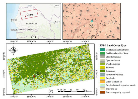
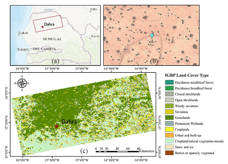
Dahra is a town of commune status located in the Louga region of Senegal at roughly 264 km from Dakar, with a center latitude of 15°21′N and a center longitude of 15°36′W. The region has a tropical climate with pleasant heat throughout the year, with well-defined dry and humid seasons that result from the northeast winter winds and the southwest summer winds. The dry season is from December to April and the wet season is from roughly May to October. Located in the northwest part of the Ferlo Basin, our study area, as shown in Figure 1, is a sandy pastoral region, where the predominant soil types are red-brown sandy soils and ferruginous tropical sandy soils, which is covered by open shrub steppes and grasslands. According to Tappan et al. and Cissé et al. [34,35], tree and shrub canopy cover does not exceed 5% of the total area on average, and the pseudo-steppe consists of a discontinuous herbaceous cover of annual grasses.
The in situ measurements of surface soil moisture were provided by the International Soil Moisture Net (ISMN [36]), and measured by the ThetaProbe ML2x sensor. The precision of the volumetric soil moisture is approximately ±1%. Together with precipitation and soil temperature, the values were recorded with a 1-h interval at the study site from 4 July 2002 to 1 January 2016. Both the soil temperature and the volumetric soil moisture from a depth of 5 cm at 19:00 UTC were used in the experiment, which coincidence with the acquisition time of Sentinel-1A.
2.2. Remote Sensing Datasets
2.2.1. Sentinel-1A Dataset
Sentinel-1 is a C-band (5.4 GHz) imaging radar mission consisting of two polar orbiting satellites. Sentinel-1A was first launched on 3 April 2014 followed by Sentinel-1B two years later. From 2 March 2015 to 27 November 2016, 47 scenes of Level 1 Sentinel-1A (S1A) Ground Range Detected (GRD) products were acquired in interferometric wide swath (IW) mode, with a swath width of 250 km, a ground resolution of 5 × 20 m2, dual polarization (VV-HV), and an incident angle ranges from 31 to 46°. All of the observations are on descending orbits, which pass over the study site at around 19:00 UTC. The acquired images were first radiometrically corrected to retrieve the backscattering coefficients and then processed by a 7 × 7 refined Lee filter to suppress the speckle noise. When considering the processing efficiency, the images were resampled to a 1-km pixel spacing. Image registration was the last step.
2.2.2. Global Soil Moisture Products
To better evaluate the performance of the soil moisture retrieved by the Sentinel-1A dataset, several typical microwave soil moisture products were selected for comparison and evaluation at a coarse resolution, including SMOS, SMAP, ASCAT, and AMSR-2. To ensure that the different products were compatible, the above products were resampled to 0.25° and were registered to the AMSR2 grid.
Launched on 2 November 2009, SMOS’s L-band Microwave Imaging Radiometer with Aperture Synthesis (MIRAS) radiometer picks up microwave emissions from the Earth’s surface to map levels of land soil moisture and ocean salinity. SMOS scans the global surface twice every three days at 6:00 a.m. (ascending) and 6:00 p.m. (descending) equatorial local crossing time [37]. The SMOS Level 3 daily soil moisture product with a resolution of 25 km on descending orbit was used in this study (http://www.catds.fr/Products/Products-access).
SMAP was launched on 31 January 2015 with radar and radiometer sensors both in the L-band at full polarization carried on the spacecraft. The instruments share a rotating 6-m mesh reflector antenna on a platform in a 685-km sun-synchronous near-polar orbit, viewing the Earth’s surface at a constant 40-degree incidence angle with a 1000-km swath width [38]. The mission intends to provide a capability for the global mapping of soil moisture and landscape freeze/thaw state with a maximum revisit time of three days. However, the radar sensor failed in July 2015. Therefore, only the SMAP Level 3 passive soil moisture product with a resolution of 36 km at 6:00 A.M. local time was used in this study (https://nsidc.org/data/smap/smap-data.html).
AMSR2, which continues the observations of AMSR-E, was launched on 18 May 2012 on the Global Change Observation Mission (GCOM)-W1 satellite. It operates at multiple dual-polarized frequencies ranging from 6.9 to 89 GHz in an ascending (13:30 local time) and descending (01:30 local time) mode. When compared with AMSR-E, the new mission has a larger main reflector (2.0 m), additional channels at the C-band (7.3 GHz), an improved calibration system, and an increased reliability [39,40]. The AMSR-2 Level 3 soil moisture product in descending mode was used in this study (http://gcom-w1.jaxa.jp/index.html).
The Advanced SCATterometer (ASCAT) is a radar instrument onboard the Meteorological Operational Platform (Metop) series of satellites: Metop-A was launched in October 2006 and Metop-B in September 2012; the third and last satellite (Metop-C) is expected to be launched in 2018 superseding Metop-A [41]. The radar operates in the C-band (5.255 GHz) at VV polarization and scans the Earth’s surface in a descending (9:30 local time) and ascending (21:30 local time) mode. The ASCAT soil moisture is estimated using the method developed by Technische Universität Wien (TU Wien) [42,43,44], which provides a soil moisture fraction between completely dry conditions (0%) and full saturation (100%) for the topsoil. The ASCAT Level 2 soil moisture product with a resolution of 25 km on ascending orbit was used in this study (https://www.eumetsat.int/website/home/Data/Products/Land/index.html). To allow for a comparison with the other products, the ASCAT measurements were converted to volumetric soil moisture using the soil texture information.
2.2.3. Auxiliary Datasets
The auxiliary datasets that were used in the study included soil texture, temperature, elevation, normalized difference vegetation index (NDVI), and land-cover classification datasets. The soil texture information was obtained from the Harmonized World Soil Database (HWSD [45]) provided by the Food and Agriculture Organization (FAO), which is a 30 arc-second raster database with over 15,000 different soil mapping units that combines existing regional and national updates of soil information worldwide. The bulk density and the fraction of clay and sand were extracted from the database for the experiments, and registered to the Sentinel-1A images with a resolution of 1 km. Temperature, NDVI, and land-cover classification information of the study site were extracted from Moderate Resolution Imaging Spectroradiometer (MODIS) Level 3 products. The MODIS products were the Terra surface temperature product of 1 km resolution, the Terra 16-day composite NDVI product of 250 m resolution, and the combined International Geosphere Biosphere Programme (IGBP) land-cover product of 500 m resolution. The Shuttle Radar Topography Mission (SRTM) [46] 90 m digital elevation data were used to acquire the elevation information. All of the above auxiliary data were resampled and registered to the Sentinel-1A images with a resolution of 1 km.
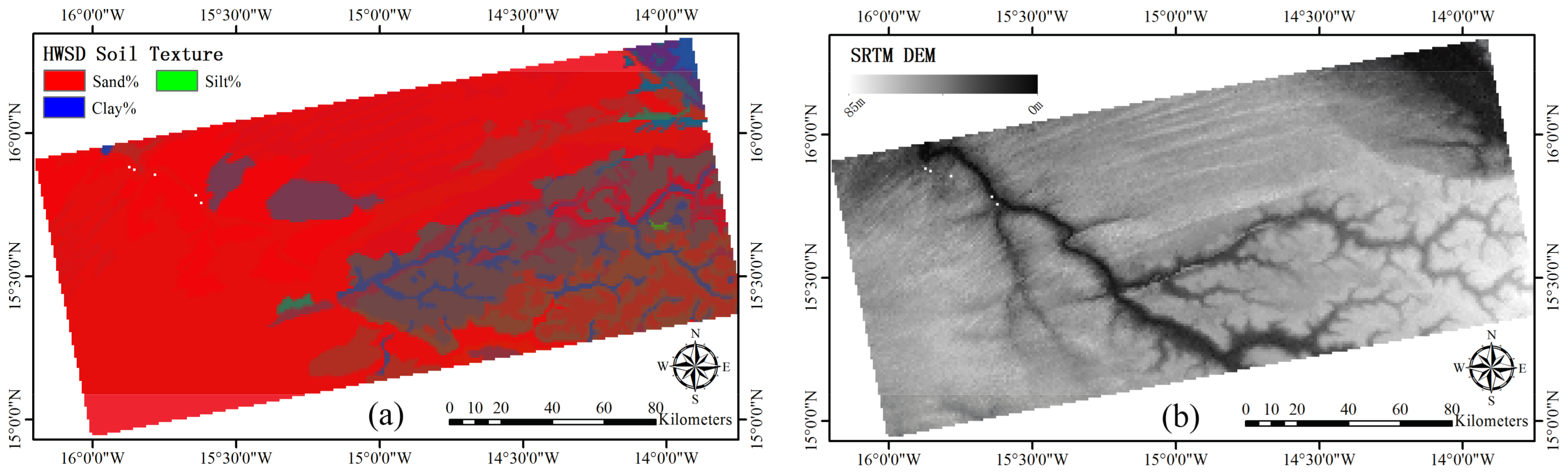
To help with the understanding of the following spatiotemporal analysis, statistical metrics, and spatial distribution of the soil texture and elevation are shown in Table 1 and Figure 2, respectively. The region is dominated by sandy soil, for which the maximum fraction of sand reaches as high as 94%. The fraction of clay in the soil is higher in the southeast and northeast. The terrain is relatively flat with an average elevation of 46.2 m and a standard deviation of 12.9 m in the study site.
2.3. Soil Moisture Retrieving Algorithm
The LUT representation of a complicated forward model has been demonstrated to be an accurate and fast tool for retrieval [47]. This approach is also applied in the SMAP mission as a baseline algorithm for the radar observations [47], and it simplifies the forward model by the soil dielectric constant, the soil surface roughness, and the vegetation water content due to the limited observation channels. By adopting a fine interval of LUT axis, this approach avoids the rather complex retrieval process of the numerical or analytical methods, while achieving similar retrieval accuracy and retaining the same retrieval formula as the forward model. Therefore, we used the LUT approach to estimate the soil moisture of the S1A images, which is similar to the baseline algorithm of the SMAP mission. The approach is divided into the following two steps: Step one: Construct the simulated data cube. In this study, the backscattering coefficients were simulated by the AIEM [48] and the Michigan microwave canopy scattering (MIMICS) [49] model for the soil and vegetation layers, respectively. Only the VV polarization was simulated for the data cube because the HV polarization is not well simulated by the AIEM. The radar configurations in the forward models were a frequency of 5.4 GHz and incident angles ranging from 30 to 46°, with an interval of 2°. Instead of characterizing the soil roughness by just the root-mean-squared height (), a discrete combination of and correlation length () was set as one axis of the data cube, where ranged from 0.5 to 5 cm with an interval of 0.1 cm, and the ranged from 5 to 55 cm with an interval of 10 cm. The volumetric soil moisture ranged from 0.03 to 0.45 m3/m3, with an interval of 0.01 m3/m3, and was converted to the soil dielectric constant using the Hallikainen method [50]. The vegetation factor was characterized by the vegetation water content (VWC), which ranged from 0.02 to 3.6 kg/m2.
Step two: Retrieve the soil moisture based on the LUT approach. The cost function is constructed as follows:
where and are the backscattering coefficients of the VV polarization from the S1A images and the data cube, respectively; and, are the soil dielectric constants of the S1A time-series. In the function, VWC is estimated using a set of land-cover–based equations for the NDVI and stem factors. The full details of the VWC estimation are available in the SMAP Vegetation Water Content Ancillary Data Report [51]. Supposing that soil roughness and are time-invariant throughout the observation period, then corresponding to the minimal value of the cost function are the desired soil dielectric constants. The obtained dielectric constants were then converted to volumetric soil moisture with the Hallikainen method using the soil texture information from the HWSD.
2.4. Evaluation Method
The S1A soil moisture was evaluated in both the temporal and spatial dimensions. In-situ measurements are normally considered as the reference and are used in the evaluation of the original 1-km resolution S1A soil moisture (S1A_1K) in the temporal dimension. When considering that there is only one observation station in our study, the microwave products of SMAP, SMOS, ASCAT, and AMSR2 were used in the evaluation of the S1A soil moisture in the spatial dimension. Due to the differences in resolutions, an average of S1A_1K in the AMSR-2 0.25° grid (S1A_0.25) was produced to match the coarse resolutions of the products in the evaluation. The root-mean-square difference (RMSD), which signifies the closeness of two independent datasets representing the same phenomenon, is the most commonly used error characterization in the evaluations of retrieved soil moisture. As reported by Willmott et al. [52] and Pratola et al. [53], RMSD varies with the variability within the distribution of the error magnitudes and with the square root of the number of data, as well as with the mean average deviation (MAD). Due to the differences in spatial scale representativity and the number of observations of the microwave soil moisture, the RMSD is generally affected by bias. Therefore, in addition to MAD measuring the absolute deviation from the in situ reference and the Pearson’s correlation coefficient (R) for the correlation analysis, the unbiased root-mean-squared deviation (ubRMSD) was also used in the evaluation to achieve a more reliable and comprehensive estimation of the error. The metrics are formulated as follows, where and are the soil moisture acquired from retrieval and in situ, respectively; is the number of coincident observations:
2.5. Spatiotemporal Analysis
EOF analysis was used in this study to characterize the soil moisture pattern. EOF analysis decomposes a dataset into a series of orthogonal spatial patterns, which can be correlated with regional characteristics, such as soil texture, vegetation fraction, and topography factors [26,54]. A dataset for EOF analysis typically consists of a set of observations (e.g., soil moisture) for locations that have been observed times. The dataset is described by a matrix with dimensions (). An eigenanalysis is conducted using the covariance matrix of the dataset. The principal components (PCs) are given in the columns of vector , which is calculated using:
where is obtained from the equation with , is the matrix containing the eigenvalues and is the matrix containing the eigenvectors. The eigenvectors, which are also called EOFs for simplicity, are treated as the spatial patterns in the analysis. The PCs describe how aligned the spatial patterns are with the variability at each time point. As in principal component analysis, the first EOF explains the largest portion of the total soil moisture variance, followed by the second, third, and the remaining EOFs. The portion of the variance explained by an EOF is obtained by dividing the respective eigenvalue by the sum of all the eigenvalues. To decide the reasonable number of significant EOFs that are used in this study, a North test [55] for the statistical significance of each EOF was conducted. A significance test with a 95% confidence interval was used to determine the error range of the eigenvalues :
where is the number of the time series. If the difference between the two adjacent eigenvalues is not less than the error range above, the corresponding EOF is considered as effective.
To investigate the soil moisture patterns and their relationships with geophysical factors, all of the time-varying observations, i.e., soil moisture, NDVI, and temperature datasets, were applied in the EOF analysis. With each EOF representing a spatial pattern, the percentage of variance that an EOF explains indicates the relative importance of this spatial pattern when compared with the others. When associated with PCs, we can determine the relative importance of the corresponding spatial pattern (EOF) over time: the higher the PC value, the more important the corresponding EOF at the specific time. Finally, the correlation analysis was carried out between the EOFs of soil moisture and the geophysical factors to study the controls on the retrieved soil moisture in this region.
3. Results
3.1. Evaluation of Sentinel-1A Soil Moisture
3.1.1. Microwave Soil Moisture vs. In Situ Measurements
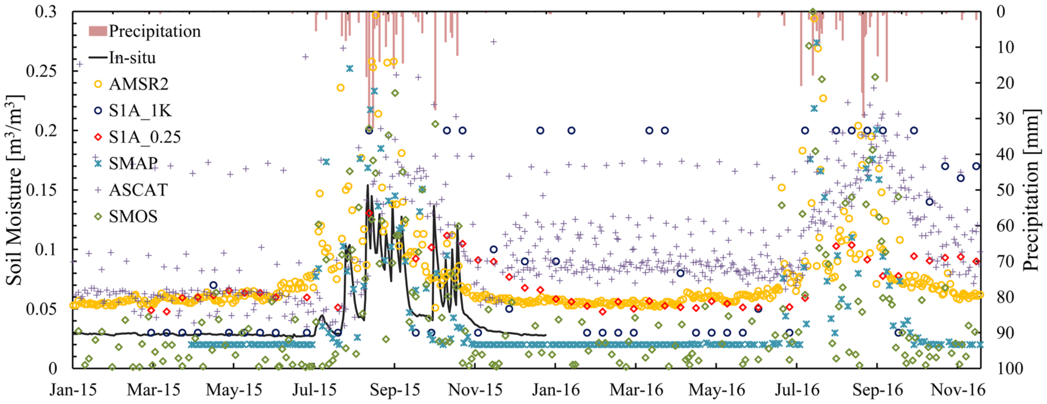
The temporal evolutions of the different soil moisture products and the daily accumulated precipitation at the test site are shown in Figure 3. The wet and dry season in our study site can be clearly identified by the precipitation and the in situ soil moisture: high values occur from July to November and low values occur from December to June. In general, the microwave soil moisture, including S1A, shows similar trends to the in situ measurements. SMAP and SMOS are the most similar among all of the soil moisture products, and they also have a better agreement with the in situ soil moisture over the whole period. ASCAT, AMSR2, and S1A_0.25 match the in situ measurements well in the wet season, but they overestimate the soil moisture by about 0.03 m3/m3 in the dry season. The finer-resolution soil moisture, i.e., S1A_1K, shows a good agreement most of the time, but shows some overestimations during the dry season. The correlation and error of the microwave soil moisture products are shown in Table 2. High agreements with the in situ measurements can be seen for SMAP, SMOS, and S1A_0.25, with R values of greater than 0.7 and a ubRMSE of less than 0.04 m3/m3, among which S1A_0.25 has the lowest ubRMSE of 0.018 m3/m3. S1A_1K has a ubRMSE of 0.053 m3/m3, which is comparable with AMSR2 and ASCAT.
3.1.2. S1A Soil Moisture vs. Microwave Products
As the ground measurements were insufficient for spatial evaluation, a comparison with the coarse resolution products was conducted to examine the performance of the S1A soil moisture using S1A_0.25 maps. The first two columns in Figure 4 show the soil moisture of S1A_0.25, SMAP, SMOS, ASCAT, and AMSR2, as averaged in the dry and wet seasons, respectively. All of the products show higher soil moisture in the wet season, as expected. The SMAP and SMOS soil moisture show lower values than the other products, especially in the dry season. While the soil moisture of ASCAT and AMSR2 appears to be homogeneous, the S1A_0.25 soil moisture shares a similar spatial pattern to SMAP and SMOS, in that the southeast is higher than the northwest in both the dry and wet seasons. In the dry season, the global products generally have soil moisture values of below 0.10 m3/m3, while the southeast of S1A_0.25 reaches 0.15 m3/m3. In the wet season, ASCAT and AMSR2 increase by about 0.10 m3/m3 over the whole region. The increment of SMAP and SMOS is more obvious in the east, while S1A_0.25 shows a larger increment in the west side.
The latter two columns in Figure 4 show the ubRMSD and R values of the microwave products, calculated with S1A_0.25 point by point. ASCAT, SMAP, and SMOS generally have ubRMSD values of under 0.06 m3/m3, while AMSR2 shows higher values in the west. Among the products, SMAP obtains the lowest ubRMSD, especially in the west, which shows the good temporal agreement with S1A_0.25. The Pearson’s correlation coefficient (R) maps show similar results: the correlations between SMAP and S1A_0.25 are higher than 0.8 in most of the pixels, followed by SMOS, with half of the pixels showing high correlations. AMSR2 and ASCAT seem to be less correlated with S1A_0.25 as the R values generally range from 0.2 to 0.6. The results indicate that the S1A soil moisture has better agreements in both the spatial and temporal dimensions with SMAP and SMOS.
3.2. EOF Analysis with Geophysical Data
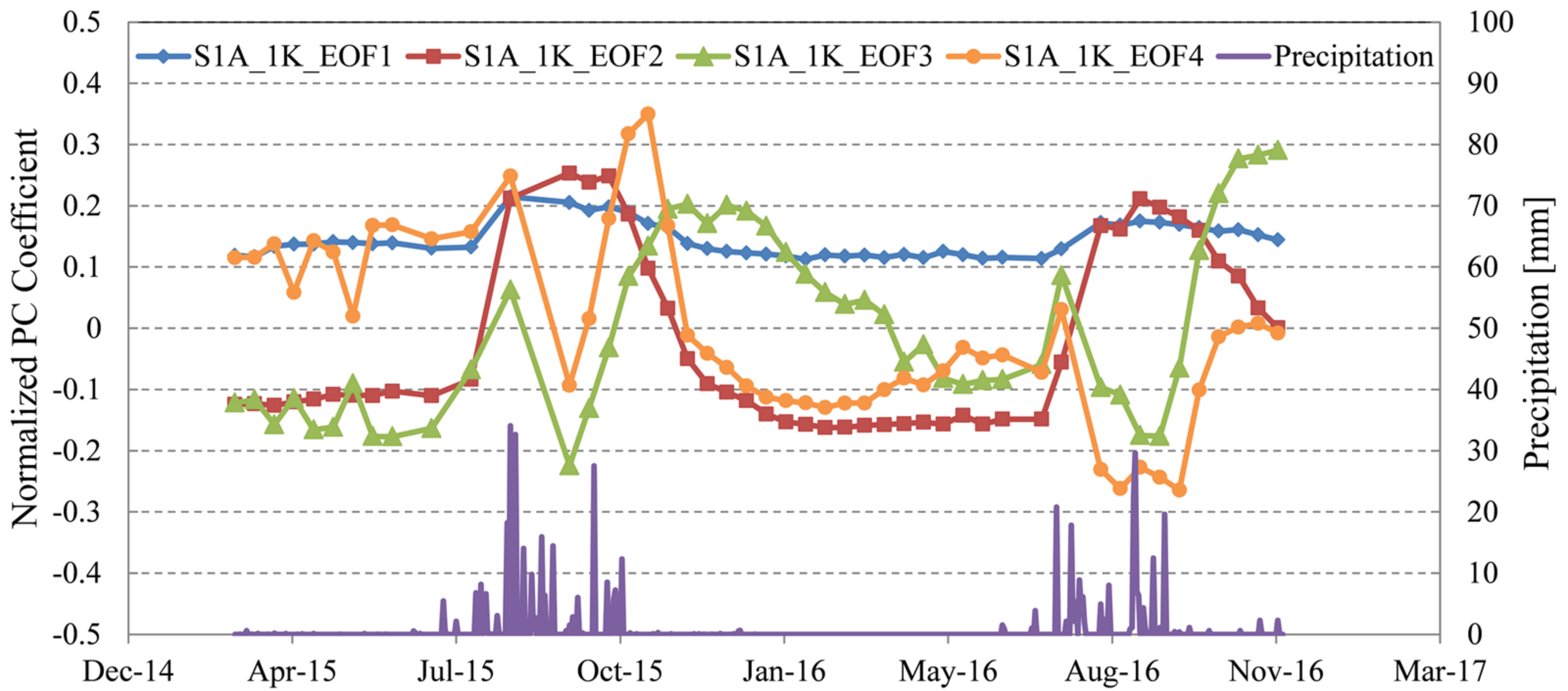
Four EOFs of the S1A_1K soil moisture, two EOFs of the MODIS NDVI, and three EOFs of the MODIS temperature remain significant after the North test. The EOFs and the corresponding PCs are shown in Figure 5, Figure 6 and Figure 7, respectively. The first four EOFs of the soil moisture explain 77.2% of the variance in total, and the primary EOF alone captures 66.2%. The results indicate that the complex pattern of S1A_1K soil moisture can be largely explained by a small number of underlying spatial structures. As the corresponding PC in Figure 6 shows no significant fluctuations, the first EOF of S1A_1K represents an averaged pattern of soil moisture: higher values gather in the southeast and northeast corner, while the southwest part shows lower values. EOF2 explains 6.2% of the total variance and is the dominant EOF in the wet seasons of 2015 and 2016, which indicates the pattern that higher soil moisture values in the northwest are more likely to occur with the increase of precipitation. The third structure, EOF3, which shows a balanced distribution, explains 2.9% of the total variance and dominates the soil moisture pattern immediately after the wet seasons. EOF4 explains 1.9% of the total variance and also shows a relatively balanced distribution, but only has a comparable dominance to EOF1 during the dry season and part of the wet season in 2015.
The primary EOF of the MODIS NDVI explains 98.3% of the total variance, which indicates that this averaged pattern dominates over the whole period. Higher values tend to concentrate in the southwest of the NDVI map. EOF2 of the NDVI only explains 0.6% of the variance and dominates the NDVI patterns in September. The temperature pattern can also be largely explained by the primary EOF with 83.4%, where the values show an increasing trend from the west to the east. This tendency is the opposite in the second EOF, which explains only 3.0% of the variance. EOF3 of the temperature shows a descending trend from the south to the north, and explains only 1.4% of the variance. As none of the three EOFs shows a significant dominance over the observation period, the spatial pattern of temperature is more complex than soil moisture and the NDVI.
The correlations between the EOFs of S1A_1K and geophysical factors were estimated by Pearson’s correlation coefficients (R), and the results are shown in Table 3. For all of the EOFs of S1A_1K, the correlations of EOF1 with the geophysical factors are obviously higher than the others, although none of the correlations are particularly high. The results show that the percentage of clay and sand show relatively higher correlations with SM_EOF1, and the EOFs of the NDVI take second place. Elevation appears to have no significant correlations with the soil moisture patterns.
4. Discussion
To better understand the spatiotemporal behavior, the evaluation of the S1A soil moisture should be as thorough as possible. However, with only one soil moisture observation station in the study site, the evaluation using the in situ measurements is limited in the spatial dimension. Therefore, comparisons with four satellite soil moisture products were adopted in this study to further evaluate the S1A soil moisture, especially in the spatial dimension. Before this could be done, an assessment needed to be undertaken to determine which of the products could better represent the in situ measurements. As is shown in the results of Section 3.1.1, SMAP and SMOS are closer to the in situ soil moisture than ASCAT and AMSR2. ASCAT has a higher ubRMSD in grassland than SMOS and SMAP [56,57,58], and more fluctuations of ASCAT soil moisture are observed in desert regions [57]. Similar fluctuations can also be seen in the temporal trend of Figure 3, especially in the dry season. AMSR2 has been reported [57] to show some overestimation in dry regions, and shows a poor performance in semiarid areas when compared with SMAP and SMOS. It also appears to largely disagree with SMAP in the soil moisture spatial patterns [37,57,59], which is a phenomenon that is also observed in both the dry and wet seasons in our study. SMAP and SMOS have been reported to be the most similar, exhibiting the lowest ubRMSD values and the highest R values overall [57,60]. In this paper, SMAP and SMOS obtain ubRMSD values of 0.038 and 0.029 m3/m3, respectively, and R values of 0.79 and 0.77, respectively, which are the lowest ubRMSD values and the highest R values among all of the products. Combining the results of previous studies [37,56,57,58,59,60], we can conclude that SMAP and SMOS are better indicators of in situ measurements for the further evaluation of S1A soil moisture in the spatial dimension.
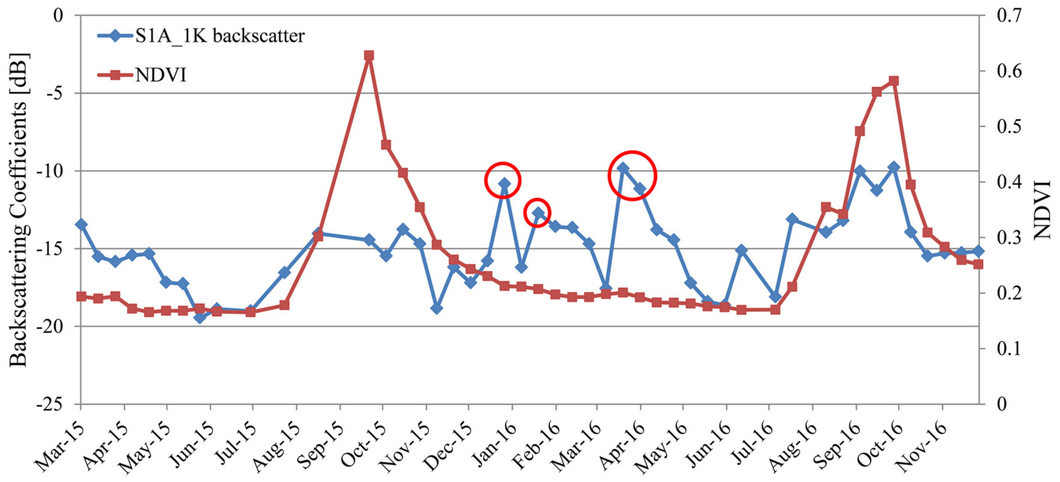
Although S1A_1K soil moisture is expected to be closer to in situ measurements because of the spatial scale, S1A_1K does not perform as well as SMAP and SMOS. As the dominant land-cover class at the Dahra site is grassland, the performance of S1A_1K could be mainly affected by the vegetation. Figure 8 shows the evolution of the backscattering coefficients and NDVI of the Dahra site, where the values in red circles correspond to severe overestimations of S1A_1K. While the NDVI is generally low in the dry seasons, the marked backscattering coefficients are even higher than the values in the wet seasons, which leads to the overestimations of S1A_1K. Nevertheless, S1A_1K reaches an acceptable accuracy, with a ubRMSD of 0.053 m3/m3 (RMSD of 0.061 m3/m3), when compared with other studies of soil moisture retrieval by Sentinel-1 images, where the RMSD of the Sentinel-1 soil moisture has ranged from 0.05 to 0.15 m3/m3 and the R value has ranged from 0.7 to 0.9. S1A_0.25 has a comparable high accuracy, although the deviations are largely eliminated by the averaging. Both S1A_1K and S1A_0.25 show good agreements of temporal trend with the precipitation and microwave products in 2016 when there are no in situ measurements. Meanwhile, S1A_0.25 shows a similar spatial distribution to SMAP and SMOS in Figure 4, which indicates that the S1A soil moisture can be considered as close enough to the real condition in the spatial dimension. The performances of the S1A soil moisture not only proves the effectiveness of the retrieval method used in this study, which does not need training or calibration, but it also shows the potential for retrieving soil moisture using time-series Sentinel-1 data.
After the evaluations in both the temporal and spatial dimensions, the spatiotemporal analysis using the EOF method could be applied to S1A_1K. According to Figure 5a and Figure 6, the primary pattern of soil moisture distribution indicates that the southwest part is drier than the others, especially in the wet seasons. This pattern has higher correlations with soil texture than the other factors and the wetter pixels tend to have a higher fraction of clay, as shown in Figure 2a and Figure 5a. The fraction of clay and sand define the infiltration and water holding capacity of the soil, and a higher proportion of clay in the soil will slow down the process of infiltration and hold more water content [32], which might be the reason for the clayey pixels having higher soil moisture values when the precipitation increases in the wet seasons. Since gravity is a driving force of the vertical flows of water into deeper levels of the ground, the topographic complexity of the study area can be assumed to impact the soil moisture pattern: for example, wetter locations tend to occur in the valley bottoms [61]. In this study site, the elevation shows no significant correlation with the distribution pattern of soil moisture. The main reason for this may be that the study area has a relatively smooth topography, which is not enough to impact the local accumulation or evaporation pattern of soil moisture. The vegetation factor is represented by the NDVI derived from MODIS. For a vegetated region, the vegetation layer covering the ground will restrict the evaporation of soil moisture and intercept the input water by the leaf, but it can also cause soil moisture loss by evaporation [32]. Medium but negative correlation is observed between the primary EOF of soil moisture and the NDVI. The primary EOF of the NDVI is dominant in the dry seasons and most of the wet seasons, with the pattern that higher values correspond to lower soil moisture pixels in the southwest and lower values correspond to higher soil moisture pixels in the other areas. This phenomenon may indicate that the loss of soil moisture is the dominant process in the vegetation region of this study area, whether by the interception of rain or restraining of the water into the soil through stem flow. Since the impact of vegetation on soil moisture is observed in Figure 8, this conclusion needs further validations. As for the temperature, it is the key factor that influences the loss of water by evaporation from soil or vegetation. However, the EOFs of temperature appear to have no significant correlations with the distribution pattern of soil moisture. Although the explanation rate of the primary EOF of temperature is rather high, no large differences in PC coefficients among the EOFs are observed. This means that there is no dominant pattern of temperature in this study area, which may result in the reduced contribution to soil moisture patterns. Previous studies have generally considered that soil moisture spatial variability is mainly affected by meteorological forcings, such as precipitation and temperature at the scale from 50 to 400 km [62,63,64], which is contradictory to the result in our study. As reported by Seneviratne et al. and Wang et al. [27,65], the effect of meteorological forcings on regional soil moisture spatial variability might become more important in regions with larger climate gradients or more homogeneous soil textures. Therefore, further studies are still necessary for the understanding of the geophysical controls on soil moisture patterns.
Although the ongoing microwave products were used for evaluation, we still cannot provide a comprehensive evaluation of S1A soil moisture (especially at 1-km resolution) due to the difference in the spatial resolution. The robustness of the retrieval algorithm that was used in this study can be further investigated using soil moisture from a land surface model or a well-designed ground sensor network as the reference. As long-term ground observations of soil moisture are increasing in number [66,67], the optimization of the sensor network starts to attract more attention. The ground measurements can be expected to represent the variability of the soil moisture in the study site [68]. Since the spatial and temporal soil moisture variability is affected by the heterogeneity of soil, vegetation, and topography [26,69], the sensor network should also have the ability of capturing the distribution of these factors. In our study area, the locations of additional sensors should be selected according to the distribution of soil moisture, soil texture, vegetation, and land covers, because the terrain is relatively flat and both the elevation and temperature have little impact on the patterns of soil moisture. Apart from different types of soil texture and land covers, the locations of the sensors could be selected with different soil moisture and NDVI levels, based on the primary spatial patterns of S1A_1K and NDVI, shown in Figure 5a,e. Vachaud et al. [70] suggested that if the measurements of soil moisture at the field were repeatedly observed, certain locations could be identified as being temporally stable. Thus, a sensor network with a temporal persistence of more than one year might provide more reliable records when considering the seasonal changes of some meteorological and geophysical factors (e.g., precipitation and vegetation, as shown in Figure 3 and Figure 8). To identify the representative locations for the validation of remote sensing soil moisture, temporal stability analysis (TSA) has been widely used in previous research [71,72,73]. The basic principle of TSA is that a location that demonstrates the ability to capture the mean of the field with a small bias (low mean relative difference: MRD) and low variability (i.e., low standard deviation of the relative difference: SDRD) would be a representative station [74]. Since the EOFs and the corresponding PCs of S1A_1K represent different spatial patterns and their variability in the observation period, the EOF analysis might also be able to characterize the temporal stability of soil moisture. Therefore, further evaluation of Sentinel-1 soil moisture based on a well-designed sensor network will be investigated in our future work.
5. Conclusions
In this study, the soil moisture at Dahra in Senegal was retrieved using S1A time-series data. The LUT method was used for the retrieval, with the backscattering coefficients being simulated based on the MIMICs and the AIEM. The evaluation of S1A soil moisture with regard to the temporal trend and spatial variation was conducted based on ground measurements and microwave products, respectively. The S1A soil moisture shows a good agreement with the temporal trend of ground measurements at the Dahra site and shows a similar spatial pattern at a coarse resolution to SMAP and SMOS, which are regarded as the best representatives of ground measurements among the microwave products. Because of the insufficient ground measurements, the retrieving algorithm needs more data to confirm its robustness over various land covers. Despite this, the preliminary results will support further studies of Sentinel-1 for soil moisture monitoring. The EOF analysis was conducted to investigate the spatiotemporal pattern of S1A soil moisture. For the geophysical control factors, it was found that the local factors of soil and vegetation are more correlated with the primary soil moisture pattern, while none of these factors have dominant controls on the soil moisture patterns in this area, due to the complexity of the regional water cycle. The discussion in this paper confirms that it is possible to retrieve and study the spatiotemporal patterns of soil moisture using time-series Sentinel-1 data, which will become more time continuous with the constellation of Sentinel-1A and Sentinel-1B.
Acknowledgments
The authors would like to thank the National Natural Science Foundation of China (No. 91438203, No. 61371199, No. 41501382, No. 41601355, No. 41771377); Hubei Provincial Natural Science Foundation (No. 2015CFB328, No. 2016CFB246); National Basic Technology Program of Surveying and Mapping (No. 2016KJ0103); and Technology of target recognition based on GF-3(No. 03-Y20A10-9001-15/16). The authors would also like to thank the reviewers and editors for their professional suggestions.
Author Contributions
Pingxiang Li contributed materials; Zhiqu Liu and Jie Yang conceived and designed the experiments; Zhiqu Liu performed the experiments; Zhiqu Liu, Jie Yang and Pingxiang Li analyzed the data; Zhiqu Liu and Jie Yang wrote the paper. All of the authors contributed to the editing of the manuscript.
Conflicts of Interest
The authors declare no conflict of interest.
References
- Pierdicca, N.; Fascetti, F.; Pulvirenti, L.; Crapolicchio, R.; Muñoz-Sabater, J. Analysis of ASCAT, SMOS, in-situ and land model soil moisture as a regionalized variable over Europe and North Africa. Remote Sens. Environ. 2015, 170, 280–289. [Google Scholar] [CrossRef]
- Gherboudj, I.; Magagi, R.; Berg, A.A.; Toth, B. Characterization of the spatial variability of in-situ soil moisture measurements for upscaling at the spatial resolution of RADARSAT-2. IEEE J. Sel. Top. Appl. Earth Obs. Remote Sens. 2017, 10, 1813–1823. [Google Scholar] [CrossRef]
- Rötzer, K.; Montzka, C.; Vereecken, H. Spatio-temporal variability of global soil moisture products. J. Hydrol. 2015, 522, 187–202. [Google Scholar] [CrossRef]
- Bai, X.; He, B.; Li, X.; Zeng, J.; Wang, X.; Wang, Z.; Zeng, Y.; Su, Z. First assessment of Sentinel-1A data for surface soil moisture estimations using a coupled Water Cloud Model and Advanced Integral Equation Model over the Tibetan Plateau. Remote Sens. 2017, 9, 714. [Google Scholar] [CrossRef]
- Kornelsen, K.C.; Coulibaly, P. Advances in soil moisture retrieval from synthetic aperture radar and hydrological applications. J. Hydrol. 2013, 476, 460–489. [Google Scholar] [CrossRef]
- Petropoulos, G.P.; Ireland, G.; Barrett, B. Surface soil moisture retrievals from remote sensing: Current status products & future trends. Phys. Chem. Earth 2015, 83, 36–56. [Google Scholar] [CrossRef]
- Barrett, B.W.; Dwyer, E.; Whelan, P. Soil moisture retrieval from active spaceborne microwave observations: An evaluation of current techniques. Remote Sens. 2009, 1, 210–242. [Google Scholar] [CrossRef]
- Kerr, Y.H.; Waldteufel, P.; Wigneron, J.P.; Delwart, S.; Cabot, F.; Boutin, J.; Escorihuela, M.J.; Font, J.; Reul, N.; Gruhier, C.; et al. The SMOS mission: New tool for monitoring key elements of the global water cycle. Proc. IEEE 2010, 98, 666–687. [Google Scholar] [CrossRef] [Green Version]
- Entekhabi, D.; Njoku, E.G.; O’Neill, P.E.; Kellogg, K.H.; Crow, W.T.; Edelstein, W.N.; Entin, J.K.; Goodman, S.; Jackson, T.; Johnson, J.; et al. The soil moisture active passive (SMAP) mission. Proc. IEEE 2010, 98, 704–716. [Google Scholar] [CrossRef]
- Bartalis, Z.; Wagner, W.; Naeimi, V.; Hasenauer, S.; Scipal, K.; Bonekamp, H.; Figa, J.; Anderson, C. Initial soil moisture retrievals from the METOP-A Advanced Scatterometer (ASCAT). Geophys. Res. Lett. 2007, 34. [Google Scholar] [CrossRef]
- Su, C.H.; Ryu, D.; Young, R.I.; Western, A.W.; Wagner, W. Inter-comparison of microwave satellite soil moisture retrievals over the Murrumbidgee Basin, southeast Australia. Remote Sens. Environ. 2013, 134, 1–11. [Google Scholar] [CrossRef]
- Wang, H.; Allain-Bailhache, S.; Méric, S.; Pottier, E. Soil parameter retrievals over bare agricultural fields using multiangular RADARSAT-2 dataset. IEEE J. Sel. Top. Appl. Earth Obs. Remote Sens. 2016, 9, 5666–5676. [Google Scholar] [CrossRef]
- Jagdhuber, T.; Hajnsek, I.; Papathanassiou, K.P. An iterative generalized hybrid decomposition for soil moisture retrieval under vegetation cover using fully polarimetric SAR. IEEE J. Sel. Top. Appl. Earth Obs. Remote Sens. 2015, 8, 3911–3922. [Google Scholar] [CrossRef]
- Bertoldi, G.; Della Chiesa, S.; Notarnicola, C.; Pasolli, L.; Niedrist, G.; Tappeiner, U. Estimation of soil moisture patterns in mountain grasslands by means of SAR RADARSAT2 images and hydrological modeling. J. Hydrol. 2014, 516, 245–257. [Google Scholar] [CrossRef]
- Ali, I.; Greifeneder, F.; Stamenkovic, J.; Neumann, M.; Notarnicola, C. Review of machine learning approaches for biomass and soil moisture retrievals from remote sensing data. Remote Sens. 2015, 7, 16398–16421. [Google Scholar] [CrossRef]
- He, L.; Qin, Q.; Panciera, R.; Tanase, M.; Walker, J.P.; Hong, Y. An extension of the Alpha approximation method for soil moisture estimation using time-series SAR data over bare soil surfaces. IEEE Geosci. Remote Sens. Lett. 2017, 14, 1328–1332. [Google Scholar] [CrossRef]
- Pierdicca, N.; Pulvirenti, L.; Bignami, C. Soil moisture estimation over vegetated terrains using multitemporal remote sensing data. Remote Sens. Environ. 2010, 114, 440–448. [Google Scholar] [CrossRef]
- Baghdadi, N.; Gaultier, S.; King, C. Retrieving surface roughness and soil moisture from synthetic aperture radar (SAR) data using neural networks. Can. J. Remote Sens. 2002, 28, 701–711. [Google Scholar] [CrossRef]
- Moran, M.S.; Hymer, D.C.; Qi, J.; Sano, E.E. Soil moisture evaluation using multi-temporal synthetic aperture radar (SAR) in semiarid rangeland. Agric. For. Meteorol. 2000, 105, 69–80. [Google Scholar] [CrossRef]
- Zhang, X.; Chen, B.; Fan, H.; Huang, J.; Zhao, H. The Potential Use of Multi-Band SAR Data for Soil Moisture Retrieval over Bare Agricultural Areas: Hebei, China. Remote Sens. 2016, 8, 7. [Google Scholar] [CrossRef]
- Torres, R.; Snoeij, P.; Geudtner, D.; Bibby, D.; Davidson, M.; Attema, E.; Potin, P.; Rommen, B.; Floury, N.; Brown, M.; et al. GMES Sentinel-1 mission. Remote Sens. Environ. 2010, 120, 9–24. [Google Scholar] [CrossRef]
- Hornacek, M.; Wagner, W.; Sabel, D.; Truong, H.L.; Snoeij, P.; Hahmann, T.; Diedrich, E.; Doubková, M. Potential for high resolution systematic global surface soil moisture retrieval via change detection using Sentinel-1. IEEE J. Sel. Top. Appl. Earth Obs. Remote Sens. 2012, 5, 1303–1311. [Google Scholar] [CrossRef]
- Pierdicca, N.; Pulvirenti, L.; Pace, G. A prototype software package to retrieve soil moisture from Sentinel-1 data by using a bayesian multitemporal algorithm. IEEE J. Sel. Top. Appl. Earth Obs. Remote Sens. 2014, 7, 153–166. [Google Scholar] [CrossRef]
- Paloscia, S.; Pettinato, S.; Santi, E.; Notarnicola, C.; Pasolli, L.; Reppucci, A. Soil moisture mapping using Sentinel-1 images: Algorithm and preliminary validation. Remote Sens. Environ. 2013, 134, 234–248. [Google Scholar] [CrossRef]
- Alexakis, D.D.; Mexis, F.D.K.; Vozinaki, A.E.K.; Daliakopoulos, I.N.; Tsanis, I.K. Soil Moisture Content Estimation Based on Sentinel-1 and Auxiliary Earth Observation Products. A Hydrological Approach. Sensors 2017, 17, 1455. [Google Scholar] [CrossRef] [PubMed]
- Vereecken, H.; Huisman, J.A.; Pachepsky, Y.; Montzka, C.; Van Der Kruk, J.; Bogena, H.; Weihermüller, L.; Herbst, M.; Martinez, G.; Vanderborght, J. On the spatio-temporal dynamics of soil moisture at the field scale. J. Hydrol. 2014, 516, 76–96. [Google Scholar] [CrossRef]
- Wang, T.; Franz, T.E.; Li, R.; You, J.; Shulski, M.D.; Ray, C. Evaluating climate and soil effects on regional soil moisture spatial variability using EOFs. Water Resour. Res. 2017, 53, 4022–4035. [Google Scholar] [CrossRef]
- Famiglietti, J.S.; Rudnicki, J.W.; Rodell, M. Variability in surface moisture content along a hillslope transect: Rattlesnake Hill, Texas. J. Hydrol. 1998, 210, 259–281. [Google Scholar] [CrossRef]
- Zucco, G.; Brocca, L.; Moramarco, T.; Morbidelli, R. Influence of land use on soil moisture spatial–temporal variability and monitoring. J. Hydrol. 2014, 516, 193–199. [Google Scholar] [CrossRef]
- Joshi, C.; Mohanty, B.P. Physical controls of near-surface soil moisture across varying spatial scales in an agricultural landscape during SMEX02. Water Resour. Res. 2010, 46. [Google Scholar] [CrossRef]
- Yoo, C.; Kim, S. EOF analysis of surface soil moisture field variability. Adv. Water Resour. 2004, 27, 831–842. [Google Scholar] [CrossRef]
- Gaur, N.; Mohanty, B.P. Land-surface controls on near-surface soil moisture dynamics: Traversing remote sensing footprints. Water Resour. Res. 2015, 52, 6365–6385. [Google Scholar] [CrossRef]
- Su, B.; Wang, A.; Wang, G.; Wang, Y.; Jiang, T. Spatiotemporal variations of soil moisture in the Tarim River basin, China. Int. J. Appl. Earth Obs. Geoinf. 2016, 48, 122–130. [Google Scholar] [CrossRef]
- Tappan, G.G.; Sall, M.; Wood, E.C.; Cushing, M. Ecoregions and land cover trends in Senegal. J. Arid Environ. 2004, 59, 427–462. [Google Scholar] [CrossRef]
- Cissé, S.; Eymard, L.; Ottlé, C.; Ndione, J.A.; Gaye, A.T.; Pinsard, F. Rainfall Intra-Seasonal Variability and Vegetation Growth in the Ferlo Basin (Senegal). Remote Sens. 2016, 8, 66. [Google Scholar] [CrossRef] [Green Version]
- International Soil Moisture Network. Available online: https://ismn.geo.tuwien.ac.at/ismn/ (accessed on 12 April 2017).
- Chen, Y.; Yang, K.; Qin, J.; Cui, Q.; Lu, H.; La, Z.; Han, M.; Tang, W. Evaluation of SMAP, SMOS and AMSR2 soil moisture retrievals against observations from two networks on the Tibetan Plateau. J. Geophys. Res. Atmos. 2017, 122, 5780–5792. [Google Scholar] [CrossRef]
- Colliander, A.; Jackson, T.J.; Bindlish, R.; Chan, S.; Das, N.; Kim, S.B.; Cosh, M.H.; Dunbar, R.S.; Dang, L.; Pashaian, L.; et al. Validation of SMAP surface soil moisture products with core validation sites. Remote Sens. Environ. 2017, 191, 215–231. [Google Scholar] [CrossRef]
- Imaoka, K.; Maeda, T.; Kachi, M.; Kasahara, M.; Ito, N.; Nakagawa, K. Status of AMSR2 instrument on GCOM-W1. In Proceeding of the SPIE 8528, Earth Observing Missions and Sensors: Development, Implementation, and Characterization II, Kyoto, Japan, 9 November 2012. [Google Scholar]
- Zeng, J.; Li, Z.; Chen, Q.; Bi, H.; Qiu, J.; Zou, P. Evaluation of remotely sensed and reanalysis soil moisture products over the Tibetan Plateau using in-situ observations. Remote Sens. Environ. 2015, 163, 91–110. [Google Scholar] [CrossRef]
- Brocca, L.; Crow, W.T.; Ciabatta, L.; Massari, C.; de Rosnay, P.; Enenkel, M.; Hahn, S.; Amarnath, G.; Camici, S.; Tarpanelli, A.; et al. A review of the applications of ASCAT soil moisture products. IEEE J. Sel. Top. Appl. Earth Obs. Remote Sens. 2017, 10, 2285–2306. [Google Scholar] [CrossRef]
- Naeimi, V.; Scipal, K.; Bartalis, Z.; Hasenauer, S.; Wagner, W. An improved soil moisture retrieval algorithm for ERS and METOP scatterometer observations. IEEE Trans. Geosci. Remote Sens. 2009, 47, 1999–2013. [Google Scholar] [CrossRef]
- Naeimi, V.; Bartalis, Z.; Wagner, W. ASCAT soil moisture: An assessment of the data quality and consistency with the ERS scatterometer heritage. J. Hydrometeorol. 2009, 10, 555–563. [Google Scholar] [CrossRef]
- Naeimi, V.; Leinenkugel, P.; Sabel, D.; Wagner, W.; Apel, H.; Kuenzer, C. Evaluation of soil moisture retrieval from the ERS and Metop scatterometers in the lower Mekong Basin. Remote Sens. 2013, 5, 1603–1623. [Google Scholar] [CrossRef] [Green Version]
- Harmonized World Soil Database v 1.2. Available online: http://www.fao.org/soils-portal/soil-survey/soil-maps-and-databases/harmonized-world-soil-database-v12/en/ (accessed on 11 April 2017).
- SRTM 90 m Digital Elevation Database v4.1. Available online: http://www.cgiar-csi.org/data/srtm-90m-digital-elevation-database-v4-1 (accessed on 11 April 2017).
- Kim, S.B.; Moghaddam, M.; Tsang, L.; Burgin, M.; Xu, X.; Njoku, E.G. Models of L-band radar backscattering coefficients over global terrain for soil moisture retrieval. IEEE Trans. Geosci. Remote Sens. 2014, 52, 1381–1396. [Google Scholar] [CrossRef]
- Wu, T.D.; Chen, K.S. A reappraisal of the validity of the IEM model for backscattering from rough surfaces. IEEE Trans. Geosci. Remote Sens. 2004, 42, 743–753. [Google Scholar] [CrossRef]
- Ulaby, F.T.; Sarabandi, K.; McDonald, K.; Whitt, M.; Dobson, M.C. Michigan microwave canopy scattering model. Int. J. Remote Sens. 1990, 11, 1223–1253. [Google Scholar] [CrossRef]
- Hallikainen, M.T.; Ulaby, F.T.; Dobson, M.C.; El-Rayes, M.A.; Wu, L.K. Microwave dielectric behavior of wet soil-part 1: Empirical models and experimental observations. IEEE Trans. Geosci. Remote Sens. 1985, 25–34. [Google Scholar] [CrossRef]
- Soil Moisture Active Passive. Available online: https://smap.jpl.nasa.gov/documents/ (accessed on 29 December 2016).
- Willmott, C.; Matsuura, K. Advantages of the mean absolute error (MAE) over the root mean square error (RMSE) in assessing average model performance. Clim. Res. 2005, 30, 79–82. [Google Scholar] [CrossRef]
- Pratola, C.; Barrett, B.; Gruber, A.; Kiely, G.; Dwyer, E. Evaluation of a global soil moisture product from finer spatial resolution SAR data and ground measurements at Irish sites. Remote Sens. 2014, 6, 8190–8219. [Google Scholar] [CrossRef]
- Jawson, S.D.; Niemann, J.D. Spatial patterns from EOF analysis of soil moisture at a large scale and their dependence on soil, land-use, and topographic properties. Adv. Water Resour. 2007, 30, 366–381. [Google Scholar] [CrossRef]
- North, G.R.; Bell, T.L.; Chalan, R.F.; Moeng, F.J. Sampling errors in the estimation of empirical orthogonal functions. Mon. Weather Rev. 1982, 110, 699–706. [Google Scholar] [CrossRef]
- Kerr, Y.H.; Al-Yaari, A.; Rodriguez-Fernandez, N.; Parrens, M.; Molero, B.; Leroux, D.; Bircher, S.; Mahmoodi, A.; Mialon, A.; Richaume, P.; et al. Overview of SMOS performance in terms of global soil moisture monitoring after six years in operation. Remote Sens. Environ. 2016, 180, 40–63. [Google Scholar] [CrossRef]
- Burgin, M.S.; Colliander, A.; Njoku, E.G.; Chan, S.K.; Cabot, F.; Kerr, Y.H.; Bindlish, R.; Jackson, T.J.; Entekhabi, D.; Yueh, S.H. A comparative study of the SMAP passive soil moisture product with existing satellite-based soil moisture products. IEEE Trans. Geosci. Remote Sens. 2017, 55, 2959–2971. [Google Scholar] [CrossRef]
- Leroux, D.J.; Kerr, Y.H.; Al Bitar, A.; Bindlish, R.; Jackson, T.J.; Berthelot, B.; Portet, G. Comparison between SMOS, VUA, ASCAT, and ECMWF soil moisture products over four watersheds in US. IEEE Trans. Geosci. Remote Sens. 2014, 52, 1562–1571. [Google Scholar] [CrossRef] [Green Version]
- Zhang, X.; Zhang, T.; Zhou, P.; Shao, Y.; Gao, S. Validation Analysis of SMAP and AMSR2 Soil Moisture Products over the United States Using Ground-Based Measurements. Remote Sens. 2017, 9, 104. [Google Scholar] [CrossRef]
- Cui, H.; Jiang, L.; Du, J.; Zhao, S.; Wang, G.; Lu, Z.; Wang, J. Evaluation and analysis of AMSR-2, SMOS, and SMAP soil moisture products in the Genhe area of China. J. Geophys. Res. Atmos. 2017, 122, 8650–8666. [Google Scholar] [CrossRef]
- Coleman, M.L.; Niemann, J.D. Controls on topographic dependence and temporal instability in catchment-scale soil moisture patterns. Water Resour. Res. 2013, 49, 1625–1642. [Google Scholar] [CrossRef]
- Vinnikov, K.Y.; Robock, A.; Speranskaya, N.A.; Schlosser, C.A. Scales of temporal and spatial variability of mid latitude soil moisture. J. Geophys. Res. 1996, 101, 7163–7174. [Google Scholar] [CrossRef]
- Robock, A.; Schlosser, C.A.; Vinnikov, K.Y.; Speranskaya, N.A.; Entin, J.K.; Qiu, S. Evaluation of the AMIP soil moisture simulations. Glob. Planet. Chang. 1998, 19, 181–208. [Google Scholar] [CrossRef]
- Entin, J.K.; Robock, A.; Vinnikov, K.Y.; Hollinger, S.E.; Liu, S.; Namkhai, A. Temporal and spatial scales of observed soil moisture variations in the extratropics. J. Geophys. Res. 2000, 105, 11865–11877. [Google Scholar] [CrossRef]
- Seneviratne, S.I.; Corti, T.; Davin, E.L.; Hirschi, M.; Jaeger, E.B.; Lehner, I.; Orlowsky, B.; Teuling, A.J. Investigating soil moisture-climate interactions in a changing climate: A review. Earth Sci. Rev. 2010, 99, 125–161. [Google Scholar] [CrossRef]
- Robock, A.; Vinnikov, K.Y.; Srinivasan, G.; Entin, J.K.; Hollinger, S.E.; Speranskaya, N.A.; Liu, S.; Namkhai, A. The global soil moisture data bank. Bull. Am. Meteorol. Soc. 2000, 81, 1281–1299. [Google Scholar] [CrossRef]
- Dorigo, W.A.; Wagner, W.; Hohensinn, R.; Hahn, S.; Paulik, C.; Xaver, A.; Gruber, A.; Drusch, M.; Mecklenburg, S.; van Oevelen, P.; et al. The international soil moisture network: A data hosting facility for global in situ soil moisture measurements. Hydrol. Earth Syst. Sci. 2011, 15, 1675–1698. [Google Scholar] [CrossRef]
- Kerkez, B.; Glaser, S.D.; Bales, R.C.; Meadows, M.W. Design and performance of a wireless sensor network for catchment-scale snow and soil moisture measurements. Water Resour. Res. 2012, 48. [Google Scholar] [CrossRef]
- Wang, X.P.; Pan, Y.X.; Zhang, Y.F.; Dou, D.; Hu, R.; Zhang, H. Temporal stability analysis of surface and subsurface soil moisture for a transect in artificial revegetation desert area, China. J. Hydrol. 2013, 507, 100–109. [Google Scholar] [CrossRef]
- Vachaud, G.; De Silans Passerat, A.; Balabanis, P.; Vauclin, M. Temporal stability of spatial measured soil water probability density function. Soil Sci. Soc. Am. J. 1985, 49, 822–827. [Google Scholar] [CrossRef]
- Penna, D.; Brocca, L.; Borga, M.; Dalla Fontana, G. Soil moisture temporal stability at different depths on two alpine hillslopes during wet and dry periods. J. Hydrol. 2013, 477, 55–71. [Google Scholar] [CrossRef]
- Gao, X.; Wu, P.; Zhao, X.; Wang, J.; Shi, Y.; Zhang, B.; Tian, L.; Li, H. Estimation of spatial soil moisture averages in a large gully of the Loess Plateau of China through statistical and modeling solutions. J. Hydrol. 2013, 486, 466–478. [Google Scholar] [CrossRef]
- Hu, W.; Tallon, L.K.; Si, B.C. Evaluation of time stability indices for soil water storage upscaling. J. Hydrol. 2012, 475, 229–241. [Google Scholar] [CrossRef]
- Yee, M.S.; Walker, J.P.; Monerris, A.; Rüdiger, C.; Jackson, T.J. On the identification of representative in situ soil moisture monitoring stations for the validation of SMAP soil moisture products in Australia. J. Hydrol. 2016, 537, 367–381. [Google Scholar] [CrossRef]
Figure 1.
Information of the study area: (a) map of Senegal; (b) Google Earth image of the Dahra study site; and (c) International Geosphere Biosphere Programme (IGBP) land-cover types of the study area.
Figure 1.
Information of the study area: (a) map of Senegal; (b) Google Earth image of the Dahra study site; and (c) International Geosphere Biosphere Programme (IGBP) land-cover types of the study area.
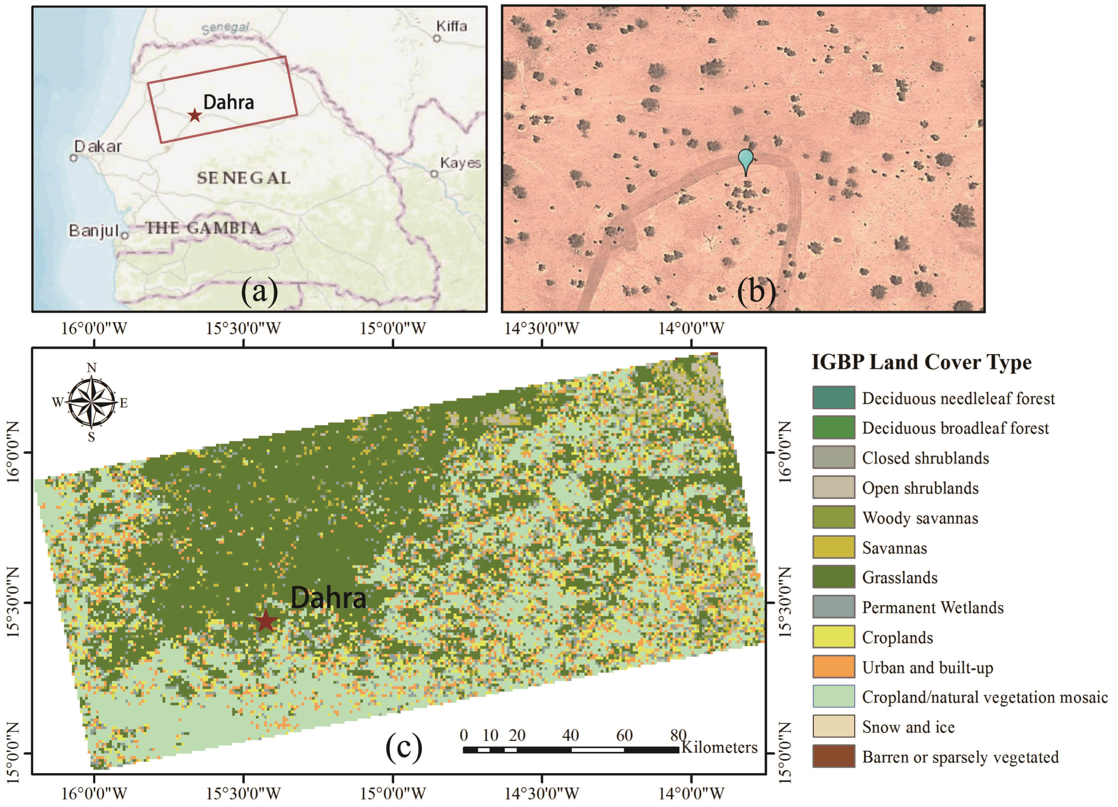
Figure 2.
Soil texture and DEM information of the Dahra study site: (a) the false-color map of soil texture taking the sandy portion as red, the silty portion as green and the clayey portion as blue; (b) Shuttle Radar Topography Mission (SRTM) DEM map.
Figure 2.
Soil texture and DEM information of the Dahra study site: (a) the false-color map of soil texture taking the sandy portion as red, the silty portion as green and the clayey portion as blue; (b) Shuttle Radar Topography Mission (SRTM) DEM map.

Figure 3.
The total daily precipitation and temporal trends of the soil moisture measurements.

Figure 4.
Comparison between S1A_0.25 and the microwave soil moisture. Column 1: the averaged soil moisture in the wet seasons; Column 2: the averaged soil moisture in the dry seasons; Column 3: the ubRMSD of the microwave products calculated with S1A_0.25 pointwise; Column 4: Pearson’s correlation coefficient (R) of the microwave products calculated with S1A_0.25 pointwise.
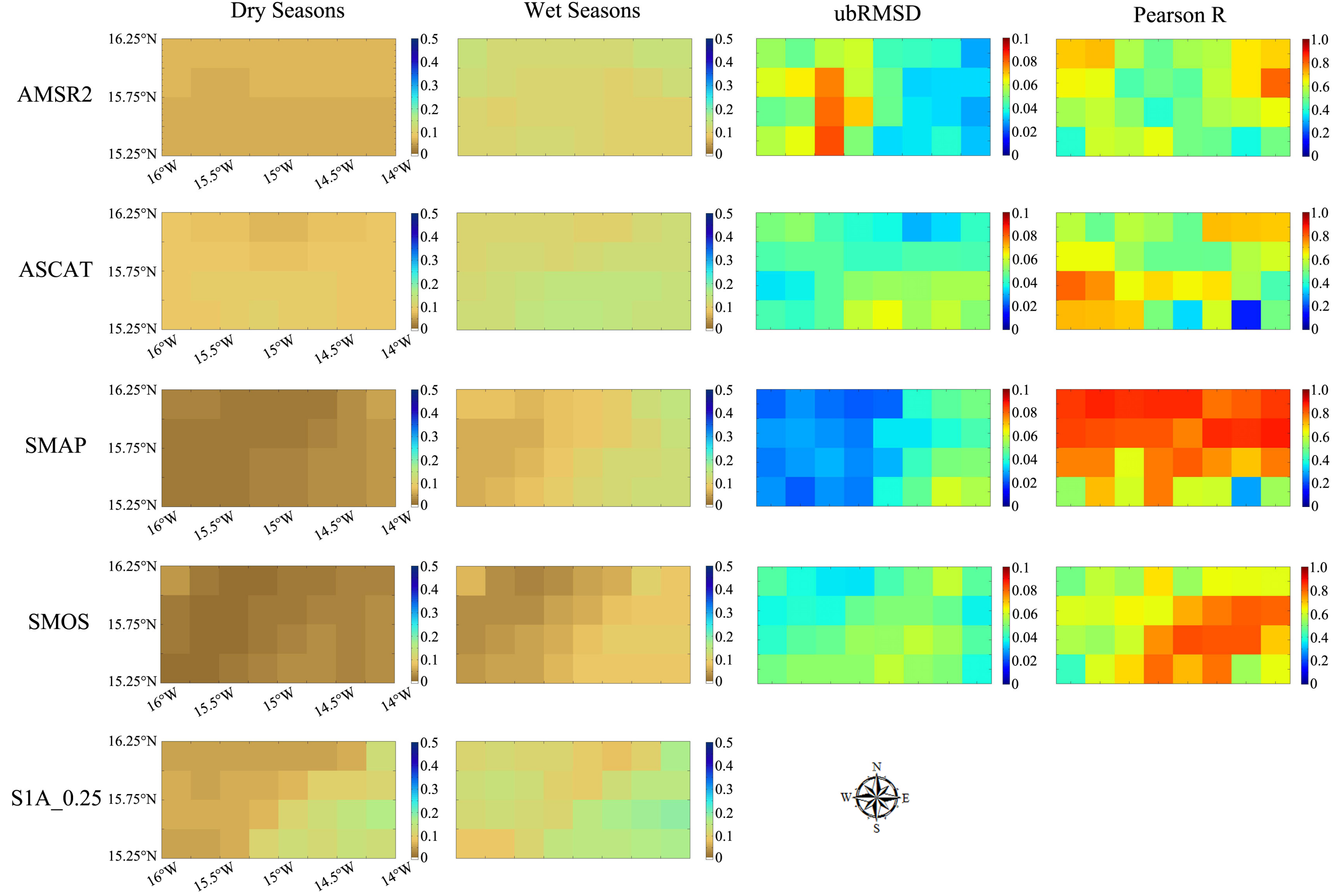
Figure 5.
The significant EOFs of S1A_1K, NDVI, and temperature. (a) The primary EOF of S1A_1K, with 66.2% of the total variance explained; (b) the 2nd EOF of S1A_1K, with 6.2% of the total variance explained; (c) the 3rd EOF of S1A_1K, with 2.9% of the total variance explained; (d) the 4th EOF of S1A_1K, with 1.9% of the total variance explained; (e) the primary EOF of NDVI, with 98.3% of the total variance explained; (f) the 2nd EOF of NDVI, with 0.6% of the total variance explained; (g) the primary EOF of temperature, with 83.4% of the total variance explained; (h) the 2nd EOF of temperature, with 3.0% of the total variance explained; and (i) the 3rd EOF of temperature, with 1.4% of the total variance explained.
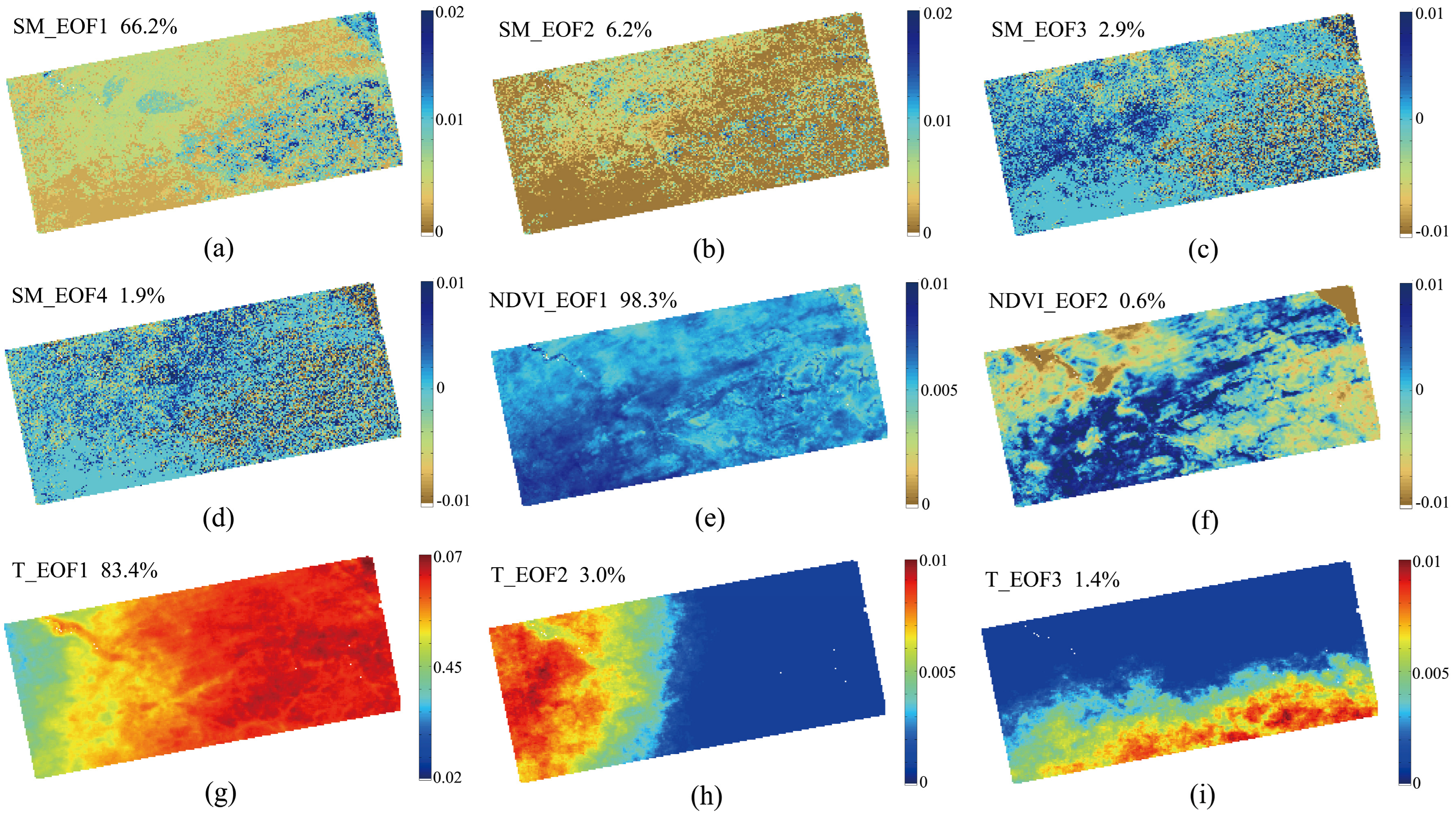
Figure 6.
The temporal evolution of corresponding principal components (PCs) for EOFs of S1A_1K.

Figure 7.
The temporal evolution of the corresponding PCs for the EOFs of normalized difference vegetation index (NDVI) and temperature.
Figure 7.
The temporal evolution of the corresponding PCs for the EOFs of normalized difference vegetation index (NDVI) and temperature.

Figure 8.
The backscattering coefficients of S1A and the NDVI at the Dahra study site. The red circles correspond to overestimations of S1A_1K.
Figure 8.
The backscattering coefficients of S1A and the NDVI at the Dahra study site. The red circles correspond to overestimations of S1A_1K.

Table 1.
The minimum (Min), maximum (Max), average (Mean), and standard deviation (SD) of the elevation and soil texture in the study area.
Table 1.
The minimum (Min), maximum (Max), average (Mean), and standard deviation (SD) of the elevation and soil texture in the study area.
| Min | Max | Mean | SD | |
|---|---|---|---|---|
| Clay | 4.0% | 63.0% | 13.2% | 11.3% |
| Sand | 11.0% | 94.0% | 74.9% | 20.4% |
| Elevation | 1.0 m | 85.0 m | 46.2 m | 12.9 m |
Table 2.
The statistical metrics of the microwave soil moisture products vs. the in situ measurements.
Table 2.
The statistical metrics of the microwave soil moisture products vs. the in situ measurements.
| S1A_1K | S1A_0.25 | SMAP | SMOS | AMSR2 | ASCAT | |
|---|---|---|---|---|---|---|
| ubRMSD | 0.053 | 0.018 | 0.038 | 0.029 | 0.052 | 0.047 |
| MAD | 0.034 | 0.035 | 0.025 | 0.024 | 0.043 | 0.055 |
| R | 0.62 * | 0.78 * | 0.77 * | 0.79 * | 0.65 * | 0.41 * |
| N | 21 | 21 | 100 | 149 | 224 | 252 |
* Significant at p < 0.05.
Table 3.
Pearson’s correlation coefficients (R)s between the empirical orthogonal functions (EOFs) of S1A_1K and geophysical factors.
Table 3.
Pearson’s correlation coefficients (R)s between the empirical orthogonal functions (EOFs) of S1A_1K and geophysical factors.
| SM_EOF1 | SM_EOF2 | SM_EOF3 | SM_EOF4 | |
|---|---|---|---|---|
| Clay | 0.48 * | −0.08 | −0.09 | −0.03 |
| Sand | −0.49 * | 0.10 | 0.10 | 0.03 |
| Elevation | 0.08 | −0.10 | −0.01 | 0.03 |
| NDVI_EOF1 | −0.40 * | −0.10 | 0.23 * | 0.10 |
| NDVI_EOF2 | −0.42 * | −0.02 | 0.10 | 0.10 |
| Temp_EOF1 | 0.28 * | −0.11 | −0.16 * | 0.02 |
| Temp_EOF2 | −0.34 * | 0.18 * | 0.16 * | 0.01 |
| Temp_EOF3 | 0.04 | −0.19 * | 0.08 | 0.01 |
* Significant at p < 0.05.
© 2017 by the authors. Licensee MDPI, Basel, Switzerland. This article is an open access article distributed under the terms and conditions of the Creative Commons Attribution (CC BY) license (http://creativecommons.org/licenses/by/4.0/).
Share and Cite
MDPI and ACS Style
Liu, Z.; Li, P.; Yang, J. Soil Moisture Retrieval and Spatiotemporal Pattern Analysis Using Sentinel-1 Data of Dahra, Senegal. Remote Sens. 2017, 9, 1197. https://doi.org/10.3390/rs9111197
AMA Style
Liu Z, Li P, Yang J. Soil Moisture Retrieval and Spatiotemporal Pattern Analysis Using Sentinel-1 Data of Dahra, Senegal. Remote Sensing. 2017; 9(11):1197. https://doi.org/10.3390/rs9111197
Chicago/Turabian StyleLiu, Zhiqu, Pingxiang Li, and Jie Yang. 2017. "Soil Moisture Retrieval and Spatiotemporal Pattern Analysis Using Sentinel-1 Data of Dahra, Senegal" Remote Sensing 9, no. 11: 1197. https://doi.org/10.3390/rs9111197
Note that from the first issue of 2016, this journal uses article numbers instead of page numbers. See further details here.