
An Improved Rotation Forest for Multi-Feature Remote-Sensing Imagery Classification

1
College of Geomatics, Shandong University of Science and Technology, Qingdao 266590, China
2
School of Remote Sensing and Information Engineering, Wuhan University, Wuhan 430079, China
*
Author to whom correspondence should be addressed.
Remote Sens. 2017, 9(11), 1205; https://doi.org/10.3390/rs9111205
Submission received: 21 September 2017
/
Revised: 19 November 2017
/
Accepted: 21 November 2017
/
Published: 22 November 2017
Abstract
:Multi-feature, especially multi-temporal, remote-sensing data have the potential to improve land cover classification accuracy. However, sometimes it is difficult to utilize all the features efficiently. To enhance classification performance based on multi-feature imagery, an improved rotation forest, combining Principal Component Analysis (PCA) and a boosting naïve Bayesian tree (NBTree), is proposed. First, feature extraction was carried out with PCA. The feature set was randomly split into several disjoint subsets; then, PCA was applied to each subset, and new training data for linear extracted features based on original training data were obtained. These steps were repeated several times. Second, based on the new training data, a boosting naïve Bayesian tree was constructed as the base classifier, which aims to achieve lower prediction error than a decision tree in the original rotation forest. At the classification phase, the improved rotation forest has two-layer voting. It first obtains several predictions through weighted voting in a boosting naïve Bayesian tree; then, the first-layer vote predicts by majority to obtain the final result. To examine the classification performance, the improved rotation forest was applied to multi-feature remote-sensing images, including MODIS Enhanced Vegetation Index (EVI) imagery time series, MODIS Surface Reflectance products and ancillary data in Shandong Province for 2013. The EVI imagery time series was preprocessed using harmonic analysis of time series (HANTS) to reduce the noise effects. The overall accuracy of the final classification result was 89.17%, and the Kappa coefficient was 0.71, which outperforms the original rotation forest and other classifier ensemble results, as well as the NASA land cover product. However, this new algorithm requires more computational time, meaning the efficiency needs to be further improved. Generally, the improved rotation forest has a potential advantage in remote-sensing classification.
1. Introduction
Frequently updated land cover data provide useful information for multi-temporal studies and are also required inputs for land cover change models, climate change models or post-catastrophe analysis [1,2]. Benefits of high-temporal frequency, remote-sensing imagery include the unique opportunity for acquiring land cover information through the process of imagery interpretation and classification [3]. To generate updated land cover data at different scales, researchers have proposed a series of remote sensing imagery classification techniques. Using the individual pixel as the basic analytical unit, the techniques can be grouped into one of three categories: unsupervised classification methods (i.e., ISODATA and K-means), supervised classification methods (i.e., decision trees, naive Bayesian, support vector machine, artificial neural network, and maximum likelihood), and hybrid classification methods (i.e., semi-supervised and fusion of supervised and unsupervised learning) [4,5]. As the spatial resolution increases quickly, object-based classification methods are proposed to address high-resolution remote-sensing images. In these methods, the pixels with homogeneous properties are grouped into basic units instead of individual pixels and the spatial contextual information is considered [6,7,8].
With the development of remote-sensing data acquisition technology, remote-sensing imagery can be easily obtained through various sensors [9]. Under these circumstances, remote-sensing classification technology faces new challenges of processing multi-source data and obtaining higher accuracy predictions [10]. The current classification techniques have respective merits and shortcomings, but different classifiers have complementary information for the correct classification results [1,11,12,13]. Therefore, one effective solution is to design classifier combinations that are either based on the same base classifiers trained on different data subsets or based on different classifiers trained on the same dataset. Schapire [14] proved that classifier combinations with a weak learning algorithm could achieve arbitrarily high accuracy. These multiple classifier systems are called classifier ensembles or multiple classifier systems (MCS) [15,16,17]. Bagging and boosting are two classical approaches for creating classifier ensembles at present. Bagging takes bootstrap samples of original objects to generate base classifiers that are used to combine the accurate ensembles. The classification result is obtained by majority voting [18]. Boosting tries to boost the performance of a “weak” classifier by using it within an ensemble structure [19]. The classifiers in the ensembles are added one at a time so that each subsequent classifier is trained on data that have been “hard” for the previous ensemble members [20]. Within this scheme, a pixel in remotely-sensed imagery could be classified using classifier ensembles to improve the accuracy. A comparison of classification performance between random forest classifier ensembles and support vector machines (SVMs) by Pal [21] indicated that random forest performs equally well to SVMs in terms of classification accuracy and training time and has even more advantages in certain aspects. Foody et al. [22] used a simple voting procedure to combine various binary classifier outputs to separate a specific class of interest from all others. Maulik and Chakraborty [23] proposed multiple classifier ensembles combining k-NN, a SVM and an incremental learning algorithm (IL) by majority voting to obtain a more accurate classification result for land cover data compared to any of the single classifiers.
Furthermore, researchers have tried many approaches to improve the performance of the classifier ensemble method. Instead of using the weights of the objects to train the next classifier, García-Pedrajas [24] used the distribution given by the weighting scheme of boosting to construct a non-linear supervised projection of the original variables. This method has been proved to achieve a better generalization error while being more robust to noise. Zhang and Zhou [25] proposed a semi-supervised ensemble method, in which the accuracy of basic learners based on labeled data was maximized, whereas the diversity among them on unlabeled data was also maximized. This method has been demonstrated to be highly competitive to other semi-supervised ensemble methods. Kim and Kang [26] utilized a neural network as a base classifier for a bagging ensemble method to obtain an improved performance over the traditional method. Rodríguez et al. [27] proposed a new classifier ensemble called rotation forest, in which the original data are projected into a new feature space using Principal Component Analysis (PCA); then, each base classifier (decision tree) is trained using the new training data for linear extracted features. The feature extraction by PCA encourages the diversity of each base classifier. The experimental results, based on hyperspectral remote-sensing imagery, revealed that rotation forest could produce more accurate results than bagging, AdaBoost, or random forest [28]. These previous studies indicate that the accuracy and diversity of base classifiers are two key features that affect the performance of the classifier ensembles [27,28,29].
Based on this finding, an improved ensemble method, drawing upon the rotation forest framework, is proposed that aims to further improve the diversity and accuracy of base classifiers. To increase the diversity of base classifiers in the ensemble, feature extraction to the subsets of features was applied by PCA, which outperforms non-parametric discriminant analysis (NDA) or random projections [29], and a full feature set for each classifier was reconstructed. The feature extraction was repeated several times, and each processing instance was able to generate different new training datasets. On each new training dataset, a boosting naïve Bayesian tree was introduced as a base classifier instead of a decision tree in the original classifier ensembles. In this new method, two-layers of voting were applied in the classification phase. We first obtained predictions using the weighted vote boosting naïve Bayesian tree; then, the majority-voting rule was used to integrate the first-layer results to obtain the final result as the prediction of the classifier ensembles. To evaluate performance, this method was applied to 2013 multi-feature remote-sensing imagery classification in Shandong Province, China.
The remainder of this paper is arranged as follows. In Section 2, we introduce the study area, data source and data filtering processing. Section 3 describes the improved classifier ensembles. Section 4 presents the experimental results and the analysis. Section 5 provides the discussion. Section 6 offers conclusions and addresses future work.
2. Study Area and Data Source
2.1. Study Area
Shandong Province is located on the eastern coast of China, and in the lower reaches of the Yellow River (34°25′–38°23′N, 114°36′–122°43′E) (Figure 1). To the east is the Bohai Sea and Huanghai Sea. The study area covers 157,100 km2, which is 1.6% of China’s total area. The western and northern area of the province is flatland plains, the central area is mountainous, and the eastern area is gentle hills. The main terrain in Shandong Province is plains, which cover 63% of the total area, followed by mountains and hills, which account for a combined 33%. This province is in a warm temperate humid and semi-humid monsoon climate. The characteristics of a marine climate are obvious in the eastern area, and the western area exhibits a continental climate. There are 17 cities in Shandong Province, and the population was 97.33 million in 2013. Industrialization and urbanization are relatively high in China. Furthermore, it is one of the major food and cotton producing areas of China.
2.2. Data Source
The MODIS datasets for Shandong Province from 2013 include the following: MOD13Q1 data version 005, MOD09Q1 data version 005 and MOD09A1 data version 005 from NASA’s Earth Observing System Data and Information System (EOSDIS). Because the Normalized Difference Vegetation Index (NDVI) in MOD13Q1 is easily saturated in the plant growth period [30], the Enhanced Vegetation Index (EVI), which overcomes this disadvantage, was chosen to track the phenological changes. The EVI has a time intervals of 16 days, so there are 23 periods of EVI data throughout the year. The land surface reflectance data consist of bands 1–2 in MOD09Q1 and bands 3–7 in MOD09A1, which were selected from September since the spectrum varies greatly during this period. Since the Normalized Differences Water Index (NDWI) has been proven to be effective in land classification in some studies [31], it was used as a feature in this study. The data are projected with the Albers Conical Equal Area format using a WGS84 coordinate system.
The ancillary data included digital elevation model (DEM) data, vegetation phenological documents and vegetation distribution imagery. The DEM data collected from a Shuttle Radar Topography Mission (SRTM) in a 90-m pixel size was resampled into a 500-m size. Vegetation phenological documents were collected from a Chinese phenology observation website. Vegetation distribution imagery on a scale of 1:1,000,000 describes the distribution of indigenous vegetation in China [32]. In this paper, the imagery was classified into six kinds of land cover categories: crop land, forest land, grass land, built-up land, water body and unused land.
2.3. EVI Data Preprocessing
In addition to cloud cover, there are other random factors, such as azimuth and elevation of the sun, moisture in the atmosphere, and aerosols, that affect the EVI data. Since the 16-day composite imagery processing cannot fully correct for these errors, the EVI images are frequently discontinuous. The errors reduce the EVI imagery accuracy and result in a lack of obvious change trends. This makes it difficult to extract useful information from the EVI.
To reduce the noise effects, harmonic analysis of time series (HANTS) [33,34,35] was performed to construct a noise-free imagery time series that is close to the reality. The fundamental principles of this filter include the notions of Fourier series and Fourier transforms. It consists of two sub-processes. One is an abnormal value identification process during which abnormal values are excluded. The other is a reconstruction process during which time series are reconstructed based on the remaining valid data.
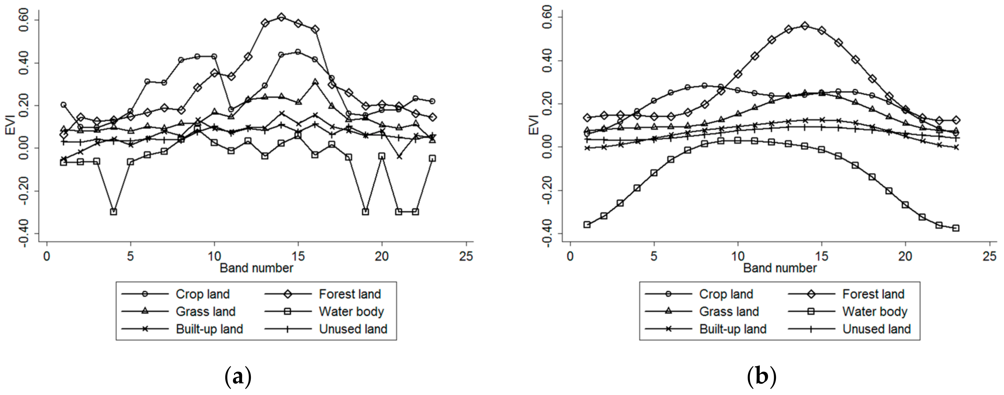
Taking the first period of EVI imagery an example, Figure 2 shows how the imagery can become much smoother after HANTS processing. The abnormal spatial patches in the original imagery are effectively filtered, and the imagery contrast is well smoothed. EVI time-varying curves (Figure 3) indicate that the noise is effectively restrained after HANTS processing while retaining the original variation trend. Moreover, the characteristics of EVI time-varying curves indicate different phenological characteristics of land cover and provide useful information to distinguish the land cover.
Based on the 32 multi-feature images (including 23 EVI images, 7 land surface reflectance images, an NDWI image and a DEM data image), the training data were selected. The Jeffries-Matusita (J-M) distance is a widely-used metric to measure the separability between classes. A J-M distance greater than 1.8 indicates good separation and less than 1.5 indicates poor separation. Table 1 and Table 2 show the J-M distance of a different couple of land cover types before and after HANTS processing. The separability between classes was significantly improved after processing, especially between vegetation classes. The J-M distance of crop-forest increased from 1.56 to 1.96. And the crop-grass J-M distance increased from 1.49 to 1.83. The forest and grass had a similar growth rhythm, so the J-M distance was lower than 1.8 but still increased higher than 1.5. The water body, built-up land and unused land all had a slight increase of separability from other classes. On the whole, the samples can be used for supervised classification.
3. Method
The rotation forest is a successful method for generating classifier ensembles based on feature extraction [27,36]. In this method, the feature set of all training samples is randomly split into K subsets (K is a parameter of the algorithm), and PCA is applied to rotate the original feature set. All of the principal components are retained to preserve the variability of information in the data. Furthermore, K-axis rotations occur to form new features for a base classifier. The diversity of each base classifier increases by feature extraction. Furthermore, the accuracy is also promoted by keeping all principal components and using the whole data set to train the base classifier.
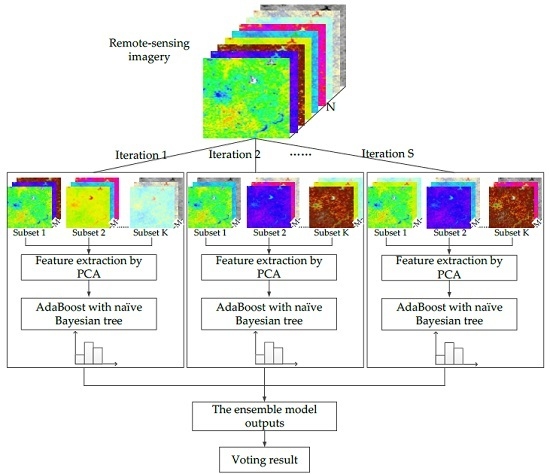
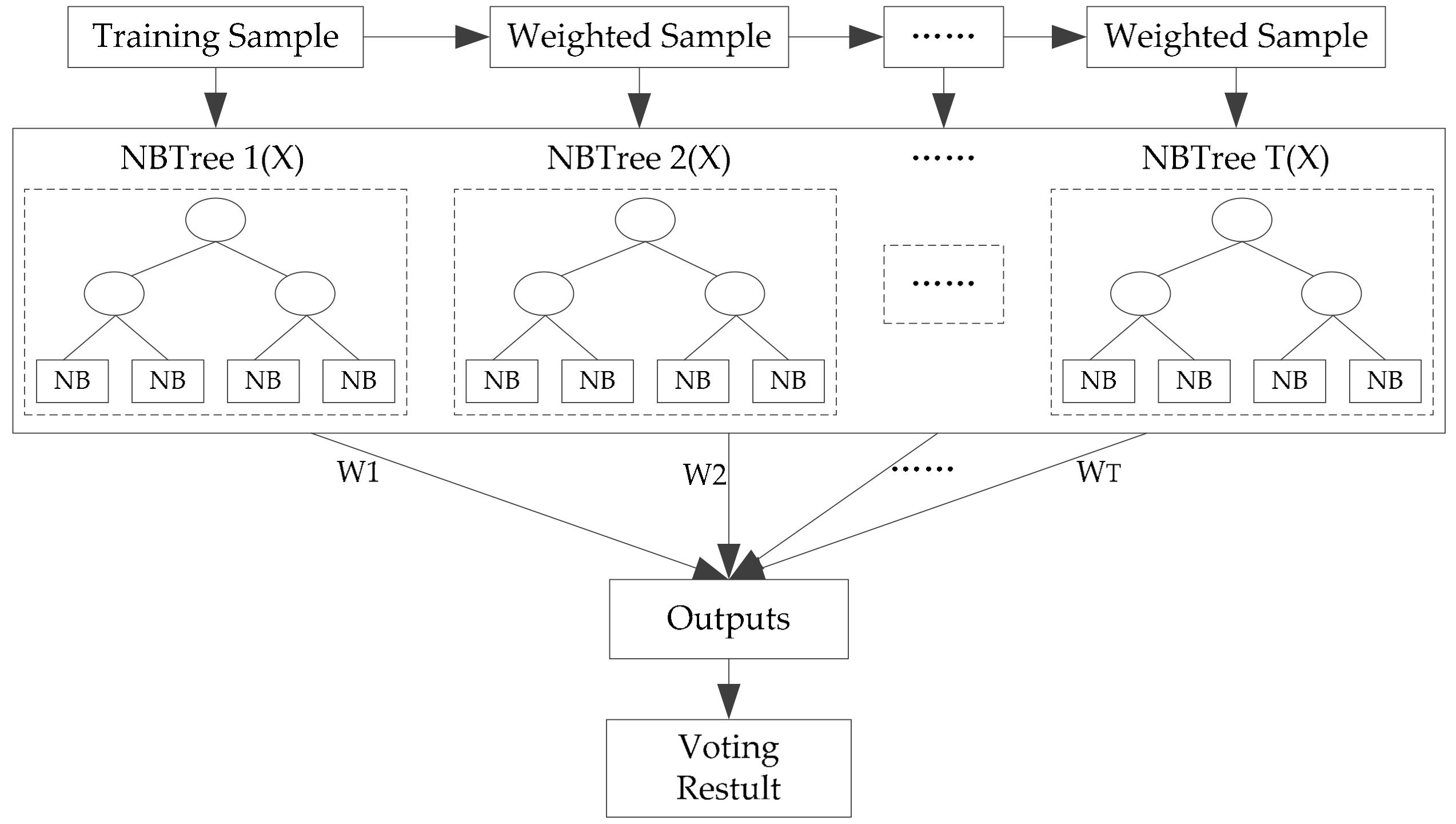
Drawing upon the rotation forest, the modified ensemble method also uses feature extraction to increase the diversity of the base classifier (Figure 4). However, different from rotation forest that employing a decision tree as a base classifier, we used the boosting naïve Bayesian tree classifier as the base classifier. The classifier ensemble, as a base classifier, could further encourage individual accuracy and achieve lower prediction error. In the classification task, we first obtained several predictions by weighted voting within a boosting naïve Bayesian tree. Then, the several prediction results were voted on to obtain the final classification result. In other words, the modified ensemble method contained two layers of voting to obtain the final result.
To simplify the notations, consider the training set containing N training objects, in which each object (xi, yi) is described by a feature vector xi = [xi1, xi2, xi3, …, xin] and a class label yi that takes a value from the set of class labels Y = {1, 2, 3, …, J}. Let C1, C2, …, CS denote S (number of classifiers) base classifiers in the ensemble, and let F denote the feature set.
To promote individual diversity within the ensemble, the reconstruction of the training set by feature extraction for classifier Cs (s = 1, 2, …, S) is conducted as follows:
- F is randomly split into K subsets (K is a number of feature subsets). The disjoint subsets are selected to maximize the diversity. Suppose K is a factor of n; then, each feature subset consists of M = n/K features.
- Xsj denotes one subset of the training dataset, which contains M features. A bootstrap sample from Xsj of 75 percent of the data count is drawn. Then, PCA is used to calculate the principal component of the new dataset. The coefficients of the principal components are stored in , an M × 1 matrix.
- Dsj is placed on the main diagonal of a zero matrix to obtain a sparse “rotation” matrix Rs as follows:
- Rearrange the columns of Rs in order to correspond to the original features order. Let denote the rearranged matrix; then, the training subset for classifier Cs is .
The feature extraction steps above are repeated S times to construct a corresponding number of classifiers.
Based on the new training dataset, for which individual diversity has been promoted, a boosting naïve Bayesian tree classifier (Figure 5) is used as the base classifier. The motivation was to increase the individual accuracy of base classifiers with the first layer voting within the ensemble. First, we briefly review the naïve Bayesian tree.
As indicated by many researchers, the instability of base classifiers is a critical factor limiting classifier ensemble accuracy [37,38,39]. To introduce instability into the boosting method, the NBTree algorithm was selected. NBTree is a hybrid of the naïve Bayesian and the Decision Tree algorithm, which integrates the advantages of the two algorithms [40,41,42]. It has the same tree-growing procedure, but the leaf nodes are a naïve Bayesian classifier. In other words, it first segments the training data by building a Top-Down Decision Tree and then builds a naïve Bayesian classifier in each subset. In this study, similar to C4.5, NBTree also uses the information gain ratio criterion to select the best test at each decision node, and the maximum depth of the tree, d, is predefined. Furthermore, NBTree does not perform pruning in this study. Because the classification of the dataset at the leaf node is not completed as the maximum depth of the tree has been predefined, the naive Bayesian method is used as the classifier. In the naïve Bayesian approach, the features are assumed to be mutually independent of each other. With this assumption, the probability of a pixel x belonging to class c can be expressed as in Equation (2):
where m is the number of features, aj is the jth feature value of x, P(c) is the prior probability and P(aj|c) is the conditional probability.
where n is the number of training objects, nc is the number of classes, ci is the class label of the ith training object, nj is the frequency of values of the jth feature, and aij is the jth feature value of the ith training object.
Taking NBTree as the base classifier, AdaBoost was used as the boosting method. AdaBoost is a sequential algorithm in which multiple classifiers are induced by adaptively changing the distribution of the training dataset based on the performance of the previously generated classifiers. Denote by Aa the new training set (, Y). Dt = [wt(1), wt(2), …, wt(M)] denotes the weight of M objects at the tth trial, where all of the mth (m = 1, 2, …, M) objects at the tth trail, wt(m), are set to be equal at first. At each trial t = 1, …, T, the boosting procedure is as follows:
- A classification model is constructed using the NBTree from Aa under the weight distribution Dt.
- In the results from step 1, if the nth object in Aa is classified correctly, let δ(m) = 0, otherwise δ(m) = 1, where δ() is part of Equation (5). The error rate of the NBTree at the tth trail is defined as follows:If εt > 0.5 or εt = 0, then the classification result is unsatisfactory; wt(m) will be reinitialized using bootstrap sampling from Aa with equal weight for each sampled object, and the boosting process continues from step 1.
- The weight vector wt+1 for the next trial is created based on the former wt.
If the mth object is classified correctly by wt(m), then
otherwise,
where Zt is a normalization factor chosen so that Dt+1 has a probability distribution over Aa. If wt+1(m) < 10−10, wt+1(m) is set to 10−10 in order to address the numerical underflow problem [43].
After T trials, the T NBTree models are combined to form a classifier ensemble. The result of each boosting NBTree is summed up by weighted voting of the predicted class in every NBTree. This is the first-layer result. Based on the obtained first-layer results, equal weight voting, which belongs to the second-layer voting, is carried out, and the final result is obtained. These classification algorithms are all run with Matlab software version 2013b.
4. Results and Analysis
In this section, the values of parameters S and T, which represent the number of iterations for feature extraction and boosting NBTree, respectively, for the improved rotation forest are first decided. Then, the effect of EVI preprocessing on classification performance is analyzed. After that, the performances of feature extraction (in this case PCA) and feature selection (in this case forward and random feature selection) in the ensemble method are compared. Last, the classification result of the improved rotation forest is compared with other classifier ensembles, as well as the corresponding NASA MODIS land cover product.
The land cover map in vector format from the land resources sectors was collected as the truthing reference data (a sample area is shown in Figure 6b). To avoid the errors caused by different classification systems, we combined the land cover types into 6 types, including crop land, forest land, grass land, built-up land, water body and unused land. Furthermore, to guarantee the accuracy and representation of reference data and to avoid the errors due to pixel resampling, approximately 25% of each land cover type of pixels were randomly selected as the sample to evaluate the accuracy of the classification result.
4.1. Optimal Combination of S and T
To investigate the effects of S and T on the performance of the improved rotation forest, we conducted experiments choosing values 1, 2, 3, …, 10 (named ST Si × Tj). For the two parameters, for example, comparison ST 2 × 3 means S = 2 and T = 3. The accuracy of the classifier with different combinations of the values for S and T were evaluated five times. The means and deviations of each different combination’s accuracy are shown in Table 3. From these results, we determined that ST 1 × 1 achieved the lowest mean accuracy. It is easy to see that ST 1 × 1 is identical to a normal naïve NBTree. With the increase in S and T, the means improved and the deviations reduced. When controlling one parameter and changing the other one, we observed that S and T have a similar effect on accuracy improvement. After ST 4 × 4, the overall accuracy tended to gradually stabilize. For the sake of prudence, we chose the combination ST 10 × 4, which has a higher mean value and less deviation than the parameters in the classification algorithm.
4.2. Effect of EVI Preprocessing
In this paper, HANTS filtering was used to construct a noise-free imagery time series that is close to the reality. The J-M distance of a different couple of land cover types before and after EVI preprocessing shows that HANTS can improve the separability between land classes. In order to verify the effects of EVI preprocessing to classification performance, two multiple-feature data (with original EVI data and with preprocessed EVI data, respectively) were classified using an improved rotation forest with the comparison ST 10 × 4. The confusion matrix between the improved rotation forest results and the reference data are shown in Table 4 and Table 5.
From both the overall accuracy and Kappa coefficient, the data with preprocessed EVI achieved better classification result. As can be seen from Table 4 and Table 5, the overall accuracy was increased by 8.07% after preprocessing. The Kappa coefficient increased from 0.59 to 0.71. For certain classes, such as forest land and grass land, the classification accuracies were greatly improved. These classes have confusing spectral changing information with original EVI, but can be well distinguished after EVI preprocessed (as shown in Figure 3). According to the results, we can clearly see that EVI preprocessing played an important role in improving classification accuracy.
4.3. Comparison between PCA and Feature Selection
In the proposed ensemble method, PCA was used as the feature extraction technique and all the multi-feature information was completely preserved in the new space of extracted features. However, an alternative approach, feature selection, can be used to select a subset [44]. The feature selection approach (like forward and random feature selection, for instance) is a special case of feature extraction. This approach represents the information in the original feature space.
In order to verify the advantage of feature extraction, we compared the performance of the feature extraction (in this case PCA) and feature selection. In this study, we considered two examples of feature selection: the forward feature selection (FFS) and the random feature selection (RFS). In the forward feature selection, we sequentially selected a number of optimal feature subsets which had the same size. For random feature selection we first randomly permuted features in the original feature set and then we split the feature set into several subsets which also had the same size. In order to ensure all features were used, the subset size was set to 4, 8 and 16, respectively. In addition, one feature set without EVI data was selected as a contrast and the subset size was set to 4. The performances were assessed by overall accuracy and Kappa coefficient (Table 6).
In Table 6, the feature sets with EVI data all performed better than those without EVI data, because the EVI data contained useful information for discrimination between land classes. With EVI data, the accuracy of random feature selection was slightly higher than forward selection technique. It might be explained that random feature selection could select more independent feature subsets than the forward feature selection. However, no large difference was noticed between the two feature selection approaches. PCA performed much better than forward and random feature selection approaches, and the best result was obtained at subset size of 8. The increasing subset size seemed not significant change the accuracy.
4.4. Comparison with Other Classification Results
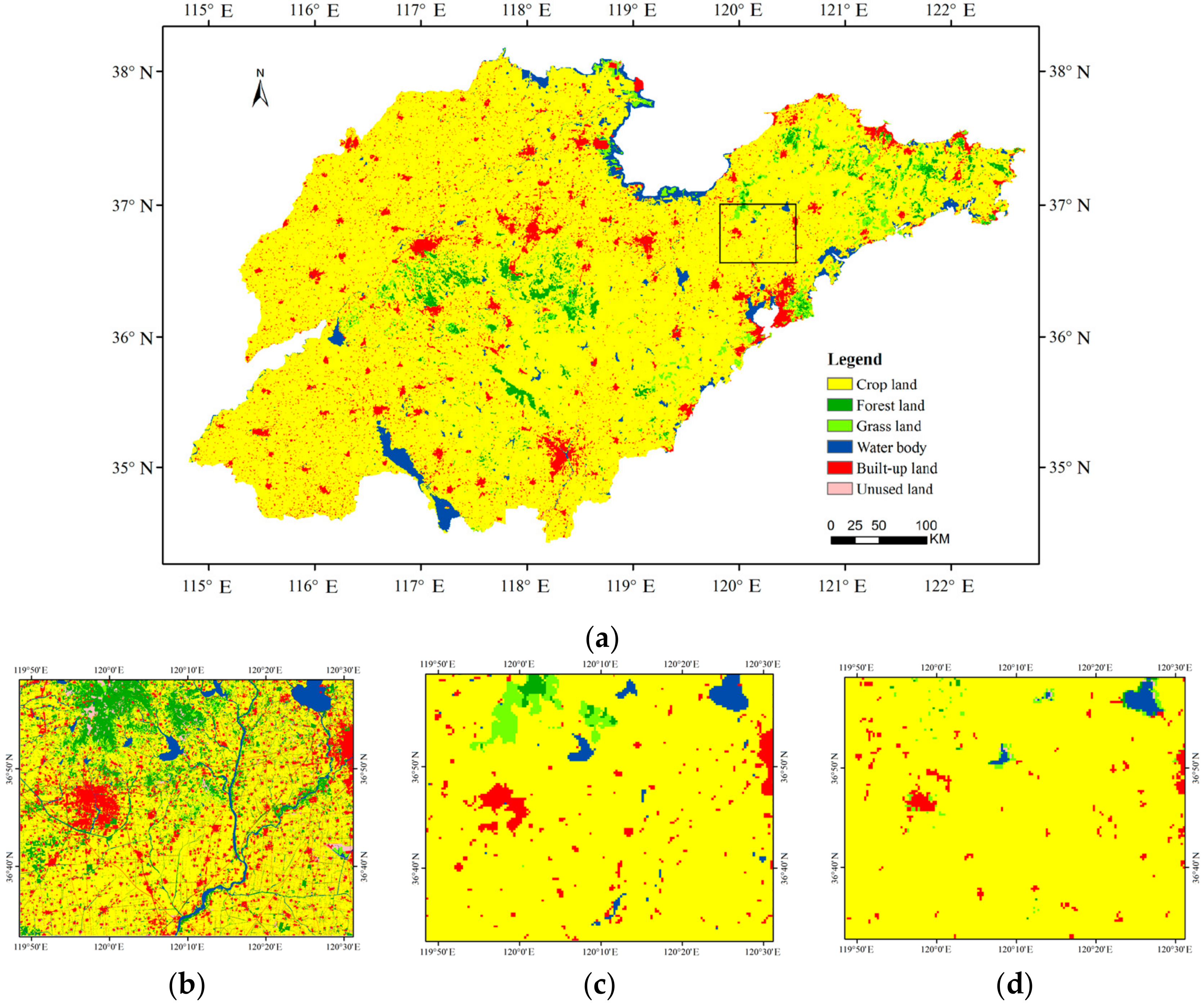
The classification result of an improved rotation forest using the comparison ST 10 × 4 is shown in Figure 6a. Crop land is the dominant land cover type and is located mainly in the plains area; because Shandong is one of the major grain-producing areas. Forest land is distributed mainly in the middle area, at higher elevations, near the Tai Mountains, and a small fraction is found on the eastern Peninsula. Large patches of built-up land aggregate in the center of every city, and rural built-up land is scattered around the cities. The proportion of grassland is small and it mainly occurs in the eastern hilly area.
Using a confusion matrix, our classification result is compared with the truthing reference data. Table 5 shows the class distribution by pixel number for each class in the reference map. The overall accuracy of our results was 89.17%, and the Kappa coefficient was 0.71. Crop land had the highest user’s accuracy, and the unused land had the lowest. This is because crop land is the main land cover type. Many built-up lands in small patches were not identified and were mistaken for crop land, as they occupy a smaller proportion in the mixed pixels in the coarse resolution imagery. Furthermore, the river having a small width was also hard to identify due to the limitation of the resolution, as sample area shown in Figure 6c.
The performances of other classifier ensembles were compared with the improved rotation forest. Furthermore, 500-m MODIS land cover product for Shandong Province from NASA (National Aeronautics and Space Administration) in 2013 was also collected (a sample area is shown in Figure 6d). The total number of iterations for the classifier ensembles was the same as for the improved rotation forest. The overall accuracy, Kappa coefficient and computation time were tested, as reported in Table 7. The computation time was measured by the native Matlab functions and was expressed in seconds. Since the MODIS land cover product is produced by NASA, the computation time is not available.
As can be seen in Table 7, the improved rotation forest obtains the highest accuracy among the compared algorithms. Using the accuracy to rank these algorithms from best to worst is the following: improved rotation forest, rotation forest, AdaBoost, Random forest, NBTree and NASA product. By comparing the results between random forest and rotation forest, we can see that feature extraction had an obvious effect on the classification accuracy improvement. However, taking into account the computation time, it has a negative effect on the efficiency because the rotation forest and improved rotation forest require the longest computation time. Because there are more procedures in the classification algorithm, the computation time increased.
The accuracy of the NASA classification result was evaluated using a confusion matrix against the reference data (Table 8). The overall accuracy was 65.96%, and the Kappa coefficient was 0.33. It is a fair agreement according to the interpretation of Kappa coefficient [45]. At the same time, the accuracy of NASA land cover data was the lowest among these classification results. In this data, the crop land was also the main land cover type. However, the forest lands in the middle of the province were not identified, and neither were the built-up lands and grass lands. Most of them were misclassified as crop land. Some water bodies near the shore were mistakenly classified as grass land or crop land. By analyzing the performance of these classification results, we found that the accuracy of the improved rotation forest result was the highest, and this improved method can provide more accurate data for land change research.
5. Discussion
In view of the fact that classifier ensembles, such as rotation forest and AdaBoost, that have been successfully applied in some remote-sensing imagery classification researches, it is plausible that a combination of the two methods may achieve lower prediction error than either of them. This paper proposed an improved rotation forest which was constructed by integrating the ideas of rotation forest and AdaBoost. The NBTree was used as the base classifier because it was more accurate than decision tree, yet sufficiently sensitive to rotation of the axes.
The high temporal resolution MODIS EVI time series, as well as ancillary geospatial and other MODIS data, were selected as the basic data. HANTS filtering was used to preprocess the EVI data. This strategy significantly increased the separability between land classes, especially the vegetation classes, and helped to improve the classification accuracy.
In order to find out which of the parameters and the feature extraction/selection methods are responsible for the good performance of improved rotation forest, multi-group comparison experiments were carried out. The sensitivity of the parameters S and T in the proposed method was investigated and the best parameters combination was selected. However, the best combination of parameters S and T was selected by enumeration. Whether there is a solution to automatically selecting an optimal combination requires further study. Then we compared the performance of feature extraction (in this study PCA) and feature selection (in this study forward and random feature selection). According to the results, no large difference was noticed between random and forward feature selection. It might be explained that in both cases all original features participated in the combined decision. Moreover, the PCA outperformed the two feature selection methods. This was because the PCA succeeded in extracting good features. When the feature extraction approach was used, all original features contribute in the new extracted feature set. The extracted features contained more useful information for discrimination between data classes. Moreover, the feature extraction encouraged individual diversity within the ensemble. On the contrary, the FFS, for instance, selected features sequentially one by one. The union of the first best feature selected with the second best one did not necessarily represent the best discriminative pair of features. By this, the selected feature subset might be not the most advantageous one. The comparison analysis demonstrated that feature extraction with PCA was more advantageous than applying feature selection techniques in the improved rotation forest. It also indicated that the dataset in this study need quite many principal components in order to obtain a classification rule that performs well due to the data distribution. However, if the first principal components succeeded in good discrimination between data classes, the classifier ensemble method on top of PCA may be not the best choice.
In addition, the increasing of the subset size from 4 to 8, and then 16 did not make the classification accuracy change significantly. Kuncheva and Rodríguez [29] had tested the impact of subset size on the rotation forest and found that there was no consistent relationship between the ensemble accuracy and subset size. In their experiment, the patterns for different data sets vary from decrease of the error with subset size, through almost horizontal lines, to increase of the error with subset size. In our study, the increasing of the subset size also did not make significant accuracy change. This was consistent with their finding. Generally, the performance of almost classifiers depends on the relation between the training sample size and the data dimensionality. The chances are the size of the training set in this study was much larger than feature space dimensionality. There is spacing between parameters of subset size in this experiment. For a thorough comparison, evaluation of the response of the improved rotation forest to the choice of each subset size is needed in the future study.
The classification result of the improved rotation forest was compared with other classifier ensembles (that is, NBTree, AdaBoost, random forest, and rotation forest). The result showed that improved rotation forest outperformed all other four methods. In fact, the improved rotation forest has a potential computational advantage over other methods in that it could parallel execute feature extraction, which preserves the variability information for the base classifier; furthermore, it combines the advantages of boosting NBTree, which could obtain an accurate result as a base classifier. An inadequacy of the method is the higher computational costs. The NASA land cover product was also collected, which had an overall accuracy of 65.96% and a Kappa coefficient of 0.33. It was unsatisfactory according to the interpretation of Kappa coefficient. The reason for this lies in two facts: one is the poor ecosystem representation of the 40–60 test sites, and the other is the implementation of algorithms that overcome previously unconsidered challenges involved in classifying high data volumes with complex feature attributes at global scales [46,47,48]. On the whole, the comparison result indicates that our classification data is more useful for land cover applications.
6. Conclusions
Multi-feature, especially multi-temporal, remote-sensing data increase the potential for discriminating different land cover types. However, addressing multiple features remains a challenge in remote-sensing classification. Satisfactory classification results not only depend on basic data with little noise but also on a classification method that performs well.
In this paper, an improved rotation forest was developed to make full use of multiple feature information. HANTS processing was applied for EVI preprocessing to increase the separability between land classes and help to improve classification accuracy. Different feature extraction/selection methods were investigated for the construction of improved rotation forests. It was shown that PCA is more advantageous than feature selection techniques to create training data for a base classifier. Based on the newly generated dataset, AdaBoost with NBTree was adopted as the base classifier to further promote the accuracy. Finally, the classification result was obtained using two-step voting. The classification result of improved rotation forest was compared with other similar classifier ensembles and NASA land cover product. The results showed that improved rotation forest outperformed the other methods. The improvement of prediction accuracy was obtained with negligible increase in computational costs. Generally, the good performance that we identified mainly depended on a high-precision pixel-wise classifier, as well as a better understanding of local land systems, including the phenological rules and the terrain data.
Nevertheless, there are still some shortcomings and problems requiring further investigation. In this study, the pixels were treated as the objects, while neglecting the spatial information effects on the rotation analysis of the remote-sensing images [49,50]. Future studies could incorporate spatial information into the improved rotation forest. Furthermore, there are other unstable algorithms, such as a neural network, that could be adopted as the base classifier in AdaBoost. It would be worthwhile to evaluate the effect of other base classifiers in the classifier ensemble on the classification accuracy.
Acknowledgments
The paper was supported by the National Statistical Science Research Project (No. 2016LY76), the China Postdoctoral Science Foundation (No. 2015M572061) and the General Program of Shandong Natural Science Foundation (No. ZR2015FM014).
Author Contributions
Yingchang Xiu designed the methodology of research, coordinated the implementation of the proposed approach, and wrote the paper; Wenbao Liu and Wenjing Yang contributed to implementing the approach and preparing the data and illustrative figures.
Conflicts of Interest
The authors declare that there is no conflict of interests regarding the publication of this article.
References
- Jia, K.; Li, Q.Z.; Tian, Y.C.; Wu, B.F. A review of classification methods of remote sensing imagery. Spectrosc. Spectr. Anal. 2011, 31, 2618–2623. [Google Scholar] [CrossRef]
- Li, M.; Zang, S.; Zhang, B.; Li, S.; Wu, C. A review of remote sensing image classification techniques: The role of spatio-contextual information. Eur. J. Remote Sens. 2014, 47, 389–411. [Google Scholar] [CrossRef]
- Alajlan, N.; Bazi, Y.; Melgani, F.; Yager, R.R. Fusion of supervised and unsupervised learning for improved classification of hyperspectral images. Inform. Sci. 2012, 217, 39–55. [Google Scholar] [CrossRef]
- Zhang, G.; Cao, Z.; Gu, Y. A hybrid classifier based on rough set theory and support vector machines. Fuzzy Syst. Knowl. Discov. 2005, 3613, 1287–1296. [Google Scholar] [CrossRef]
- Atkinson, P.M.; Lewis, P. Geostatistical classification for remote sensing: An introduction. Comput. Geosci. 2000, 26, 361–371. [Google Scholar] [CrossRef]
- Myint, S.W.; Gober, P.; Brazel, A.; Grossman-Clarke, S.; Weng, Q. Per-pixel vs. object-based classification of urban land cover extraction using high spatial resolution imagery. Remote Sens. Environ. 2011, 115, 1145–1161. [Google Scholar] [CrossRef]
- Xia, J.; Chanussot, J.; Du, P.; He, X. Spectral-spatial classification for hyperspectral data using rotation forests with local feature extraction and Markov random fields. IEEE Trans. Geosci. Remote 2015, 53, 2532–2546. [Google Scholar] [CrossRef]
- Kalra, K.; Goswami, A.K.; Gupta, R. A comparative study of supervised image classification algorithms for satellite images. Int. J. Electr. Electron. Data Commun. 2013, 1, 10–16. [Google Scholar]
- Al-Ahmadi, F.S.; Hames, A.S. Comparison of four classification methods to extract land use and land cover from raw satellite images for some remote arid areas, kingdom of Saudi Arabia. Earth 2009, 20, 167–191. [Google Scholar] [CrossRef]
- Nair, M.; Bindhu, J.S. Supervised techniques and approaches for satellite image classification. Int. J. Comput. Appl. 2016, 134, 1–6. [Google Scholar] [CrossRef]
- Zhang, Y. Ten years of technology advancement in remote sensing and the research in the CRC-AGIP lab in GCE. Geomatica 2010, 64, 173–189. [Google Scholar]
- Lu, D.; Weng, Q. A survey of image classification methods and techniques for improving classification performance. Int. J. Remote Sens. 2007, 28, 823–870. [Google Scholar] [CrossRef]
- Allwein, E.L.; Schapire, R.E.; Singer, Y. Reducing multiclass to binary: A unifying approach for margin classifiers. J. Mach. Learn. Res. 2000, 1, 113–141. [Google Scholar] [CrossRef]
- Schapire, R.E. The strength of weak learnability. Mach. Learn. 1990, 5, 197–227. [Google Scholar] [CrossRef]
- Benediktsson, J.A.; Chanussot, J.; Fauvel, M. Multiple classifier systems in remote sensing: From basics to recent developments. Mult. Classif. Syst. 2007, 4472, 501–512. [Google Scholar] [CrossRef]
- Steele, B.M. Combining multiple classifiers: An application using spatial and remotely sensed information for land cover type mapping. Remote Sens. Environ. 2000, 74, 545–556. [Google Scholar] [CrossRef]
- Doan, H.T.X.; Foody, G.M. Increasing soft classification accuracy through the use of an ensemble of classifiers. Int. J. Remote Sens. 2007, 28, 4609–4623. [Google Scholar] [CrossRef]
- Breiman, L. Bagging predictors. Mach. Learn. 1996, 24, 123–140. [Google Scholar] [CrossRef]
- Freund, Y.; Schapire, R.E. A decision-theoretic generalization of on-line learning and an application to boosting. J. Comput. Syst. Sci. 1997, 55, 119–139. [Google Scholar] [CrossRef]
- Bailly, J.S.; Arnaud, M.; Puech, C. Boosting: A classification method for remote sensing. Int. J. Remote Sens. 2007, 28, 1687–1710. [Google Scholar] [CrossRef]
- Pal, M. Random forest classifier for remote sensing classification. Int. J. Remote Sens. 2005, 26, 217–222. [Google Scholar] [CrossRef]
- Foody, G.M.; Boyd, D.S.; Sanchez-Hernandez, C. Mapping a specific class with an ensemble of classifiers. Int. J. Remote Sens. 2007, 28, 1733–1746. [Google Scholar] [CrossRef]
- Maulik, U.; Chakraborty, D. A robust multiple classifier system for pixel classification of remote sensing images. Fundam. Inform. 2010, 101, 286–304. [Google Scholar] [CrossRef]
- García-Pedrajas, N. Supervised projection approach for boosting classifiers. Pattern Recogn. 2009, 42, 1742–1760. [Google Scholar] [CrossRef]
- Zhang, M.L.; Zhou, Z.H. Exploiting unlabeled data to enhance ensemble diversity. Data Min. Knowl. Discov. 2013, 26, 98–129. [Google Scholar] [CrossRef]
- Kim, M.J.; Kang, D.K. Ensemble with neural networks for bankruptcy prediction. Expert Syst. Appl. 2010, 37, 3373–3379. [Google Scholar] [CrossRef]
- Rodríguez, J.J.; Kuncheva, L.I.; Alonso, C.J. Rotation forest: A new classifier ensemble method. IEEE Trans. Pattern Anal. 2006, 28, 1619–1630. [Google Scholar] [CrossRef] [PubMed]
- Xia, J.; Du, P.; He, X.; Chanussot, J. Hyperspectral remote sensing image classification based on rotation forest. IEEE Geosci. Remote Sens. 2014, 11, 239–243. [Google Scholar] [CrossRef]
- Kuncheva, L.I.; Rodríguez, J.J. An experimental study on rotation forest ensembles. In Multiple Classifier Systems. MCS 2007. Lecture Notes in Computer Science; Haindl, M., Kittler, J., Roli, F., Eds.; Springer: Berlin/Heidelberg, Germany, 2007; Volume 4472, pp. 459–468. ISBN 978-3-54-072481-0. [Google Scholar]
- Huete, A.; Didan, K.; Miura, T.; Rodriguez, E.P.; Gao, X.; Ferreira, L.G. Overview of the radiometric and biophysical performance of the modis vegetation indices. Remote Sens. Environ. 2002, 83, 195–213. [Google Scholar] [CrossRef]
- Lu, L.; Li, X.; Dong, Q.H.; Swinnen, E.; Veroustraete, F.; Wang, J.H.; Wang, Y.M. The mapping and validation of land cover in northwest china from SPOT4-VEGETATION. J. Remote Sens. 2003, 7, 214–220. [Google Scholar] [CrossRef]
- Shixin, Z. Vegetation and Its Geographical Pattern in China: Illustration of the Vegetation Map of China (1:1000000), 1st ed.; Geological Publishing House: Beijing, China, 2007; pp. 73–80. ISBN 978-7-11-605146-1. [Google Scholar]
- Menenti, M.; Azzali, S.; Verhoef, W.; Van Swol, R. Mapping agroecological zones and time lag in vegetation growth by means of Fourier analysis of time series of NDVI images. Adv. Space Res. 1993, 13, 233–237. [Google Scholar] [CrossRef]
- Verhoef, W.; Menenti, M.; Azzali, S. Cover A colour composite of NOAA-AVHRR-NDVI based on time series analysis (1981–1992). Int. J. Remote Sens. 1996, 17, 231–235. [Google Scholar] [CrossRef]
- Jakubauskas, M.E.; Legates, D.R.; Kastens, J.H. Crop identification using harmonic analysis of time-series AVHRR NDVI data. Comput. Electron. Agric. 2002, 37, 127–139. [Google Scholar] [CrossRef]
- Zhang, C.X.; Zhang, J.S. Rotboost: A technique for combining rotation forest and adaboost. Pattern Recogn. Lett. 2008, 29, 1524–1536. [Google Scholar] [CrossRef]
- Baumgartner, D.; Serpen, G. Performance of global–local hybrid ensemble versus boosting and bagging ensembles. Int. J. Mach. Learn. Cybern. 2013, 4, 301–317. [Google Scholar] [CrossRef]
- Breiman, L. Arcing classifiers. Ann. Stat. 1998, 26, 801–824. [Google Scholar]
- Dietterich, T.G. An experimental comparison of three methods for constructing ensembles of decision trees: Bagging, boosting, and randomization. Mach. Learn. 2000, 40, 139–157. [Google Scholar] [CrossRef]
- Kohavi, R. Scaling Up the Accuracy of Naive-Bayes Classifiers: A Decision-Tree Hybrid. In Proceedings of the Second International Conference on Knowledge Discovery and Data Mining, Portland, OR, USA, 2–4 August 1996; AAAI Press: Menlo Park, CA, USA, 1996; pp. 202–207. [Google Scholar]
- Ting, K.M.; Zheng, Z. A study of adaboost with naive bayesian classifiers: Weakness and improvement. Comput. Intell. 2003, 19, 186–200. [Google Scholar] [CrossRef]
- Hssina, B.; Merbouha, A.; Ezzikouri, H.; Erritali, M. A comparative study of decision tree ID3 and C4.5. Int. J. Adv. Comput. Sci. Appl. 2014, 4, 13–19. [Google Scholar] [CrossRef]
- Bauer, E.; Kohavi, R. An empirical comparison of voting classification algorithms: Bagging, boosting, and variants. Mach. Learn. 1999, 36, 105–139. [Google Scholar] [CrossRef]
- Skurichina, M.; Duin, R.P. Combining feature subsets in feature selection. Mult. Classif. Syst. 2005, 3541, 165–175. [Google Scholar] [CrossRef]
- Viera, A.J.; Garrett, J.M. Understanding interobserver agreement: The kappa statistic. Fam. Med. 2005, 37, 360–363. [Google Scholar] [PubMed]
- Friedl, M.A.; Muchoney, D.; Mclver, D.; Gao, F.; Hodges, J.C.F.; Strahler, A.H. Characterization of north american land cover from NOAA-ABVHRR data using the EOS MODIS land cover classification algorithm. Geophys. Res. Lett. 2000, 27, 977–980. [Google Scholar] [CrossRef]
- Zhang, X.; Sun, R.; Zhang, B.; Tong, Q. Land cover classification of the North China Plain using MODIS_EVI time series. ISPRS J. Photogramm. 2008, 63, 476–484. [Google Scholar] [CrossRef]
- Friedl, M.A.; Mclver, D.K.; Hodges, J.C.; Zhang, X.Y.; Muchoney, D.; Strahler, A.H.; Woodcock, C.E.; Gopal, S.; Schneider, A.; Cooper, A.; et al. Global land cover mapping from MODIS: Algorithms and early results. Remote Sens. Environ. 2002, 83, 287–302. [Google Scholar] [CrossRef]
- Tarabalka, Y.; Benediktsson, J.A.; Chanussot, J. Spectral-spatial classification of hyperspectral imagery based on partitional clustering techniques. IEEE Trans. Geosci. Remote 2009, 47, 2973–2987. [Google Scholar] [CrossRef]
- Tarabalka, Y.; Chanussot, J.; Benediktsson, J.A. Segmentation and classification of hyperspectral images using watershed transformation. Pattern Recogn. 2010, 43, 2367–2379. [Google Scholar] [CrossRef]
Figure 1.
Study area location map.
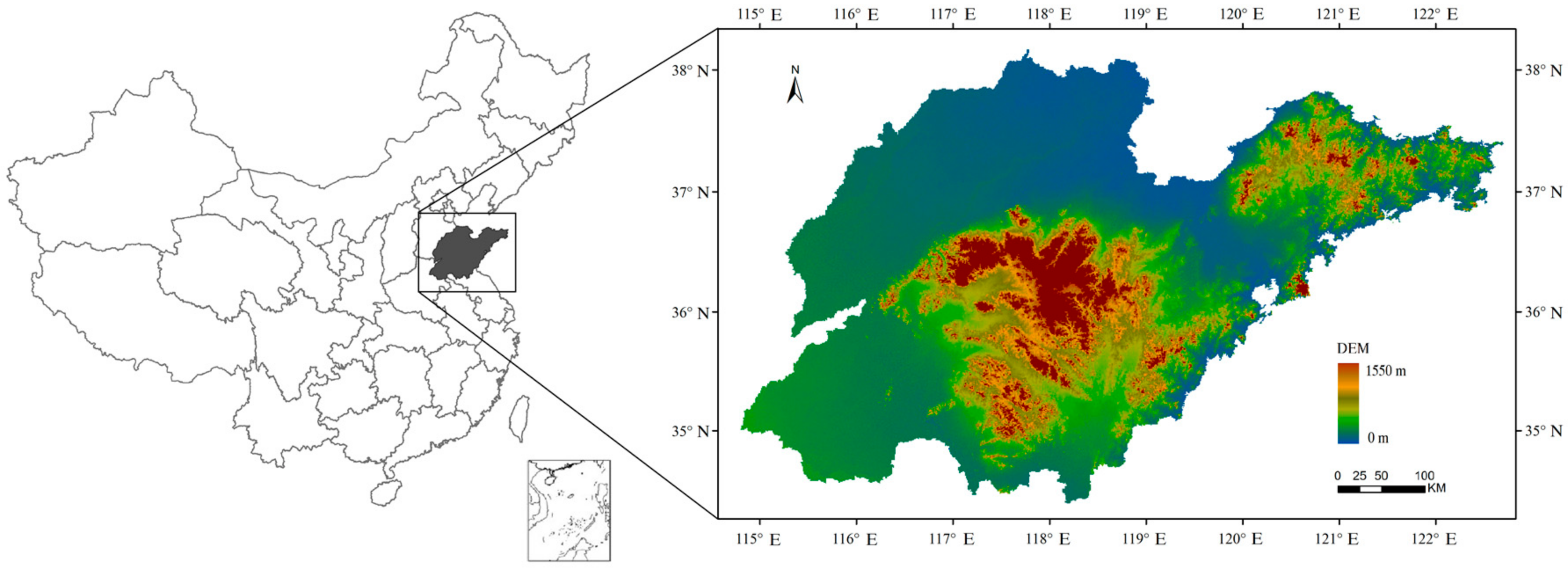
Figure 2.
Sample of imagery smoothing using HANTS processing: (a) original EVI imagery; (b) HANTS-corrected EVI imagery.
Figure 2.
Sample of imagery smoothing using HANTS processing: (a) original EVI imagery; (b) HANTS-corrected EVI imagery.
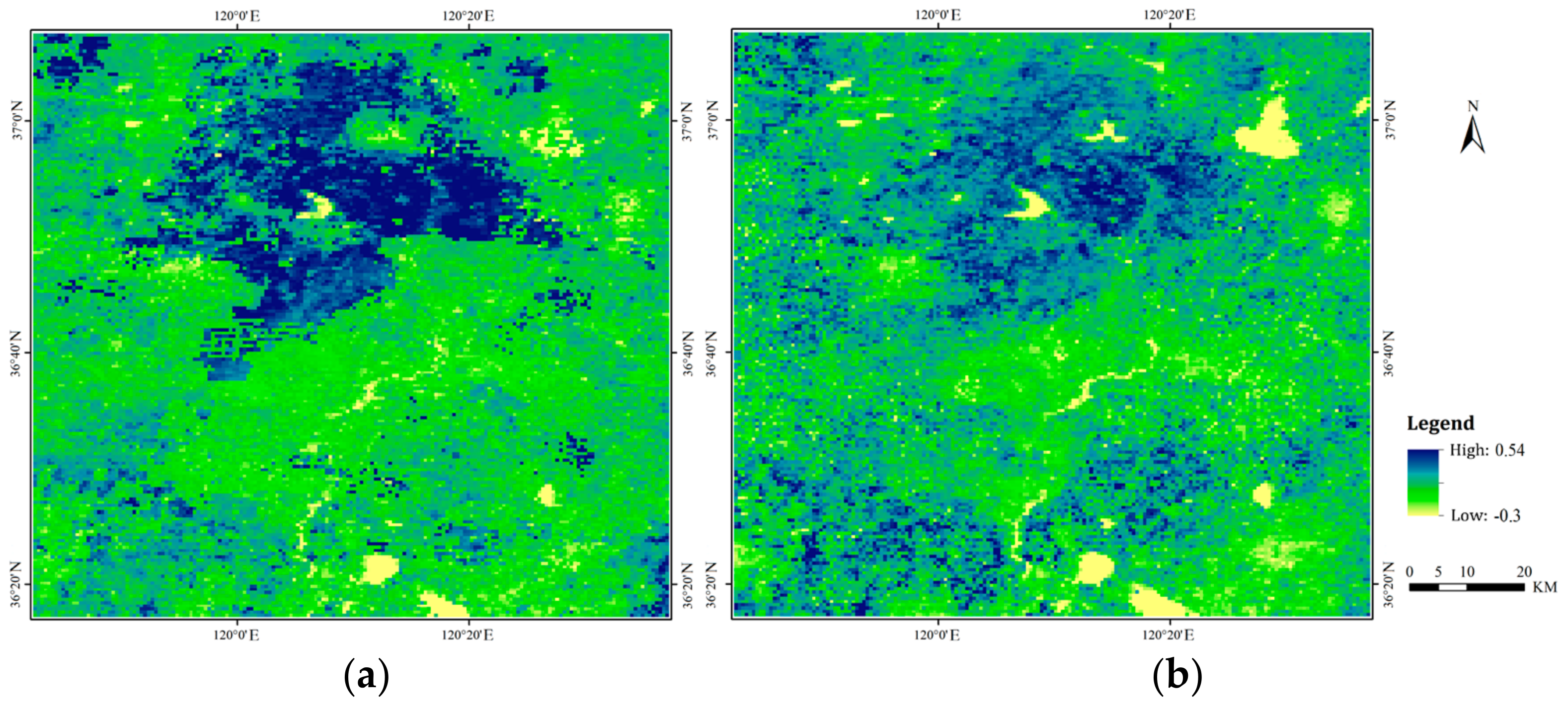
Figure 3.
EVI curves of different land cover types before and after HANTS processing: (a) original EVI curves; (b) HANTS-corrected EVI curves.
Figure 3.
EVI curves of different land cover types before and after HANTS processing: (a) original EVI curves; (b) HANTS-corrected EVI curves.

Figure 4.
Illustration of the improved rotation forest.
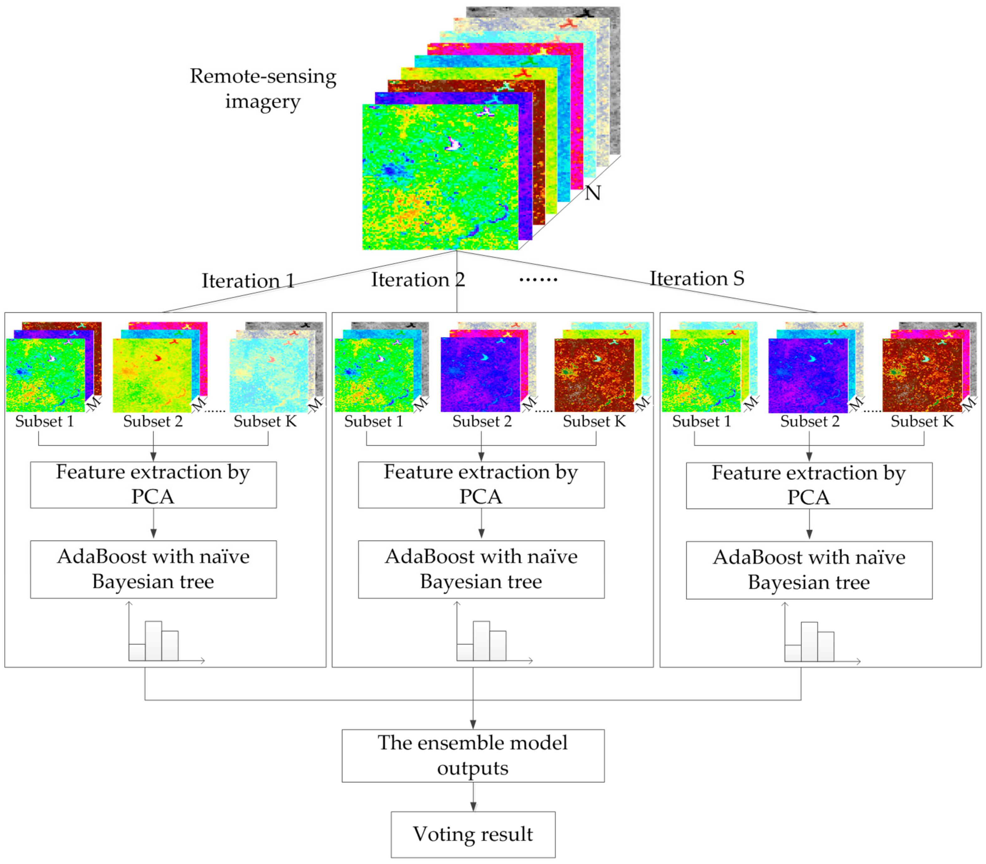
Figure 5.
Flowchart of AdaBoost with naïve Bayesian trees.

Figure 6.
Land cover classification maps: (a) improved rotation forest results for Shandong Province; (b) sample area of truthing reference map; (c) sample area of improved rotation forest results; and (d) sample area for the NASA product.
Figure 6.
Land cover classification maps: (a) improved rotation forest results for Shandong Province; (b) sample area of truthing reference map; (c) sample area of improved rotation forest results; and (d) sample area for the NASA product.

Table 1.
J-M distance between different land cover types before HANTS processing.
| Land Cover Type | Crop Land | Forest Land | Grass Land | Water Body | Built-up Land | Unused Land |
|---|---|---|---|---|---|---|
| Crop land | 1.56 | 1.49 | 1.76 | 1.75 | 1.78 | |
| Forest land | 1.53 | 1.87 | 1.76 | 1.78 | ||
| Grass land | 1.86 | 1.75 | 1.65 | |||
| Water body | 1.70 | 1.55 | ||||
| Built-up land | 1.42 | |||||
| Unused land |
Table 2.
J-M distance between different land cover types after HANTS processing.
| Land Cover Type | Crop Land | Forest Land | Grass Land | Water Body | Built-up Land | Unused Land |
|---|---|---|---|---|---|---|
| Crop land | 1.96 | 1.83 | 1.97 | 1.95 | 1.98 | |
| Forest land | 1.53 | 1.97 | 1.96 | 1.98 | ||
| Grass land | 1.96 | 1.85 | 1.85 | |||
| Water body | 1.68 | 1.65 | ||||
| Built-up land | 1.52 | |||||
| Unused land |
Table 3.
Means and deviations of test accuracy with different combinations of S and T.
| T | 1 | 2 | 3 | 4 | 5 | 6 | 7 | 8 | 9 | 10 | |
|---|---|---|---|---|---|---|---|---|---|---|---|
| S | |||||||||||
| 1 | 78.79 ± 3.37 | 80.45 ± 3.12 | 71.71 ± 6.34 | 82.93 ± 0.53 | 82.67 ± 0.70 | 81.67 ± 4.06 | 79.76 ± 5.15 | 83.13 ± 1.51 | 80.50 ± 3.08 | 79.80 ± 2.79 | |
| 2 | 77.77 ± 2.39 | 82.00 ± 1.91 | 86.39 ± 0.36 | 88.07 ± 1.17 | 87.90 ± 0.70 | 89.18 ± 0.43 | 87.09 ± 1.32 | 87.78 ± 0.35 | 88.11 ± 0.81 | 88.04 ± 0.93 | |
| 3 | 76.12 ± 1.31 | 86.81 ± 1.97 | 84.18 ± 0.53 | 85.87 ± 0.60 | 84.99 ± 0.88 | 86.11 ± 0.45 | 85.21 ± 0.91 | 87.05 ± 0.42 | 86.10 ± 0.89 | 86.33 ± 1.16 | |
| 4 | 80.32 ± 3.00 | 86.12 ± 2.34 | 85.05 ± 2.45 | 88.05 ± 0.37 | 87.73 ± 0.11 | 87.85 ± 0.86 | 87.55 ± 0.64 | 88.01 ± 0.53 | 88.45 ± 0.58 | 87.50 ± 0.11 | |
| 5 | 76.16 ± 4.22 | 86.99 ± 0.34 | 83.98 ± 2.40 | 87.26 ± 0.15 | 86.92 ± 0.28 | 87.53 ± 0.50 | 86.52 ± 0.56 | 87.42 ± 0.74 | 87.54 ± 0.33 | 86.38 ± 0.29 | |
| 6 | 81.51 ± 1.49 | 86.25 ± 1.60 | 87.16 ± 0.43 | 88.50 ± 0.17 | 88.50 ± 0.44 | 88.38 ± 0.32 | 88.04 ± 0.82 | 88.33 ± 0.74 | 88.36 ± 0.32 | 87.45 ± 0.84 | |
| 7 | 79.85 ± 0.50 | 86.13 ± 0.16 | 86.87 ± 0.39 | 88.32 ± 0.14 | 86.88 ± 1.02 | 87.31 ± 0.71 | 87.53 ± 0.43 | 87.90 ± 0.11 | 87.43 ± 0.66 | 87.07 ± 0.78 | |
| 8 | 81.29 ± 2.96 | 86.20 ± 2.49 | 86.51 ± 0.76 | 89.16 ± 0.33 | 88.03 ± 0.84 | 88.36 ± 0.50 | 88.25 ± 0.23 | 87.90 ± 0.26 | 87.95 ± 0.12 | 88.34 ± 0.32 | |
| 9 | 81.66 ± 3.11 | 87.45 ± 1.05 | 86.91 ± 0.71 | 88.70 ± 0.42 | 87.67 ± 0.69 | 88.37 ± 0.14 | 87.97 ± 0.74 | 88.16 ± 0.38 | 87.58 ± 0.17 | 88.17 ± 0.38 | |
| 10 | 83.23 ± 1.34 | 87.52 ± 0.80 | 88.00 ± 0.42 | 89.09 ± 0.10 | 88.67 ± 0.25 | 88.70 ± 0.38 | 87.88 ± 0.17 | 88.11 ± 0.34 | 88.25 ± 0.11 | 87.76 ± 0.41 | |
Table 4.
Confusion matrix between the improved rotation forest result and the reference data before EVI preprocessing.
Table 4.
Confusion matrix between the improved rotation forest result and the reference data before EVI preprocessing.
| Reference Map | ||||||||
|---|---|---|---|---|---|---|---|---|
| Result map | Land cover type | Crop land | Forest land | Grass land | Water body | Built-up land | Unused land | User’s accuracy (%) |
| Crop land | 180,735 | 5763 | 9526 | 1192 | 2417 | 154 | 90.46 | |
| Forest land | 3128 | 9929 | 1482 | 463 | 371 | 267 | 63.48 | |
| Grass land | 10,125 | 2547 | 11,918 | 1008 | 529 | 723 | 44.39 | |
| Water body | 1529 | 985 | 1028 | 9019 | 145 | 89 | 70.49 | |
| Built-up land | 4365 | 525 | 882 | 179 | 12,927 | 105 | 68.10 | |
| Unused land | 838 | 198 | 1556 | 271 | 223 | 1231 | 28.52 | |
| Producer’s accuracy (%) | 90.04 | 49.78 | 45.16 | 74.34 | 77.82 | 47.92 | ||
Overall accuracy = 81.10%; Kappa coefficient = 0.59.
Table 5.
Confusion matrix between the improved rotation forest result and the reference data after EVI preprocessing.
Table 5.
Confusion matrix between the improved rotation forest result and the reference data after EVI preprocessing.
| Reference Map | ||||||||
|---|---|---|---|---|---|---|---|---|
| Result map | Land cover type | Crop land | Forest land | Grass land | Water body | Built-up land | Unused land | User’s accuracy (%) |
| Crop land | 210,172 | 770 | 1882 | 921 | 6902 | 921 | 94.86 | |
| Forest land | 989 | 9089 | 776 | 17 | 119 | 106 | 81.91 | |
| Grass land | 2123 | 171 | 8643 | 314 | 220 | 262 | 73.66 | |
| Water body | 1360 | 557 | 1423 | 9602 | 393 | 717 | 68.33 | |
| Built-up land | 7525 | 378 | 330 | 497 | 15,157 | 116 | 63.15 | |
| Unused land | 614 | 125 | 80 | 21 | 99 | 421 | 30.96 | |
| Producer’s accuracy (%) | 94.34 | 81.96 | 65.81 | 84.44 | 66.24 | 16.56 | ||
Overall accuracy = 89.17%; Kappa coefficient = 0.71.
Table 6.
The accuracy and Kappa coefficient for FFS, RFS and PCA.
| Subset Size of 4 (Without EVI) | Subset Size of 4 | Subset Size of 8 | Subset Size of 16 | |||||
|---|---|---|---|---|---|---|---|---|
| Accuracy (%) | Kappa | Accuracy (%) | Kappa | Accuracy (%) | Kappa | Accuracy (%) | Kappa | |
| FFS | 70.88 | 0.434 | 82.63 | 0.617 | 82.67 | 0.622 | 82.68 | 0.623 |
| RFS | 71.33 | 0.472 | 82.87 | 0.621 | 82.90 | 0.627 | 82.90 | 0.625 |
| PCA | 74.48 | 0.527 | 89.12 | 0.709 | 89.17 | 0.712 | 89.16 | 0.711 |
Table 7.
Comparison of accuracy and computation time for each algorithm.
| Algorithm | Overall Accuracy (%) | Kappa Coefficient | Computation Time (s) |
|---|---|---|---|
| NASA product | 65.96 | 0.33 | N/A |
| NBTree | 79.36 | 0.55 | 0.86 |
| AdaBoost | 83.95 | 0.61 | 2.28 |
| Random forest | 83.26 | 0.60 | 3.93 |
| Rotation forest | 86.78 | 0.67 | 5.27 |
| Improved rotation forest | 89.17 | 0.71 | 7.91 |
Table 8.
Confusion matrix between the NASA product and the reference data.
| Reference Map | ||||||||
|---|---|---|---|---|---|---|---|---|
| Result map | Land cover type | Crop land | Forest land | Grass land | Water body | Built-up land | Unused land | User’s accuracy (%) |
| Crop land | 151,471 | 9177 | 8741 | 1023 | 938 | 83 | 88.36 | |
| Forest land | 3049 | 7424 | 1514 | 167 | 219 | 405 | 58.01 | |
| Grass land | 46,210 | 4146 | 9109 | 1641 | 438 | 248 | 14.74 | |
| Water body | 2560 | 767 | 1428 | 3993 | 82 | 35 | 45.04 | |
| Built-up land | 6965 | 536 | 594 | 81 | 9630 | 9 | 54.06 | |
| Unused land | 1651 | 101 | 1802 | 79 | 78 | 1978 | 34.77 | |
| Producer’s accuracy (%) | 71.48 | 33.52 | 39.28 | 57.17 | 84.59 | 71.72 | ||
Overall accuracy = 65.96%; Kappa coefficient = 0.33.
© 2017 by the authors. Licensee MDPI, Basel, Switzerland. This article is an open access article distributed under the terms and conditions of the Creative Commons Attribution (CC BY) license (http://creativecommons.org/licenses/by/4.0/).
Share and Cite
MDPI and ACS Style
Xiu, Y.; Liu, W.; Yang, W. An Improved Rotation Forest for Multi-Feature Remote-Sensing Imagery Classification. Remote Sens. 2017, 9, 1205. https://doi.org/10.3390/rs9111205
AMA Style
Xiu Y, Liu W, Yang W. An Improved Rotation Forest for Multi-Feature Remote-Sensing Imagery Classification. Remote Sensing. 2017; 9(11):1205. https://doi.org/10.3390/rs9111205
Chicago/Turabian StyleXiu, Yingchang, Wenbao Liu, and Wenjing Yang. 2017. "An Improved Rotation Forest for Multi-Feature Remote-Sensing Imagery Classification" Remote Sensing 9, no. 11: 1205. https://doi.org/10.3390/rs9111205
Note that from the first issue of 2016, this journal uses article numbers instead of page numbers. See further details here.