Combining Remote Sensing and Water-Balance Evapotranspiration Estimates for the Conterminous United States


1
Hydrologic Remote Sensing Branch, U.S. Geological Survey, Reston, VA 20192, USA
2
Earth Resources Observation and Science (EROS) Center, North Central Climate Science Center, U.S. Geological Survey, Fort Collins, CO 80523, USA
3
Earth Systems Modeling Branch, U.S. Geological Survey, Reston, VA 20192, USA
*
Author to whom correspondence should be addressed.
Remote Sens. 2017, 9(12), 1181; https://doi.org/10.3390/rs9121181
Submission received: 21 September 2017
/
Revised: 9 October 2017
/
Accepted: 2 November 2017
/
Published: 29 November 2017
(This article belongs to the Section Remote Sensing in Geology, Geomorphology and Hydrology)
Abstract
:Evapotranspiration (ET) is a key component of the hydrologic cycle, accounting for ~70% of precipitation in the conterminous U.S. (CONUS), but it has been a challenge to predict accurately across different spatio-temporal scales. The increasing availability of remotely sensed data has led to significant advances in the frequency and spatial resolution of ET estimates, derived from energy balance principles with variables such as temperature used to estimate surface latent heat flux. Although remote sensing methods excel at depicting spatial and temporal variability, estimation of ET independently of other water budget components can lead to inconsistency with other budget terms. Methods that rely on ground-based data better constrain long-term ET, but are unable to provide the same temporal resolution. Here we combine long-term ET estimates from a water-balance approach with the SSEBop (operational Simplified Surface Energy Balance) remote sensing-based ET product for 2000–2015. We test the new combined method, the original SSEBop product, and another remote sensing ET product (MOD16) against monthly measurements from 119 flux towers. The new product showed advantages especially in non-irrigated areas where the new method showed a coefficient of determination R2 of 0.44, compared to 0.41 for SSEBop or 0.35 for MOD16. The resulting monthly data set will be a useful, unique contribution to ET estimation, due to its combination of remote sensing-based variability and ground-based long-term water balance constraints.
1. Background and Rationale
Evapotranspiration (ET) is the quantity of water that includes net water evaporation and plant transpiration. It plays a significant role in the hydrologic cycle, returning about 70% of precipitation across the conterminous United States (CONUS) to the atmosphere [1,2]. Because it is generally the second largest component of the water budget, following precipitation, researchers and water resource managers require accurate and reliable ET estimates to understand water availability and distribution for both short and long-term water resources management.
The use of remote sensing-based methods of estimating ET has increased in recent years [3], and has proven useful in various applications such as agricultural water use monitoring and estimation [4], and hydrologic simulation [5]. These methods are particularly advantageous in their ability to produce estimates on timescales as short as weeks. The remote sensing approaches generally use surface energy balance arguments to partition the net incoming solar radiation energy into sensible heat flux, ground heat flux, and latent heat flux (energy equivalent of ET mass flux) [6,7,8,9,10]. Different algorithms applied to the same input remote sensing data sets can make predictions of the latent heat (ET) component as disparate as 20–60% of the available surface energy [11]. The uncertainty of ET estimation is demonstrated by the non-unique partitioning of total ET to multiple landscape sources. One study comparing this variability of ET source partitioning in three remote sensing ET algorithms showed that for the global average ET, different algorithms attributed a range of 14–52% of the ET to soil evaporation, 10–24% to evaporation of water intercepted by canopies, and 24–76% to plant transpiration [12]. Uncertainties have also been demonstrated within the energy balance algorithms due to errors in assumptions about albedo values [13]. Though there are substantial uncertainties among remote sensing ET estimates, the usefulness of the high frequency of measurements and the broad spatial coverage in capturing spatial and temporal variability mark a significant step forward in our ability to measure and monitor ET.
Physical measurements of ET are difficult to obtain. One micrometeorological method of ET measurement, eddy covariance, involves instrumenting a tower to monitor the exchange of water vapor between a local landscape of interest and the atmosphere. The AmeriFlux tower network includes data contributed from eddy covariance stations across the US (data and community background available [14]). Flux tower data represent ET measured at a point location, ideally with adequate fetch so that the measured flux at a point is indicative of flux from a given landscape type; measurements can be highly influenced by local environmental factors, with extrapolation to regional scales difficult. Flux tower data are also known to have uncertainties, with errors in their energy balance closure arguments that can be on the order of 20% [15]. However, for measurement of ET, flux tower data are currently the best available ground-truth data source at daily or monthly timescales. Analyses evaluating the accuracy of remote sensing ET estimates often involve comparisons against flux tower data, for example, for a set of 45 towers [9], 46 towers [16], or 85 towers [11]. There is a lack of studies showing comparisons using all >100 available AmeriFlux towers in the CONUS to evaluate remote sensing ET products in a variety of settings, and in relation to other variables measured at the tower locations. Such comparisons could aid in evaluation of strengths or weaknesses of different products for application in different settings, such as in irrigated areas or a given land cover type, or by month. Analyses of spatial locations of high residuals between predictions and flux tower measurements, and testing for correlations between residuals and variables such as precipitation and temperature, could also indicate potential sources of bias in products and guide algorithm refinement.
Because of the difficulty of direct measurement at larger temporal and spatial scales than represented by individual flux towers, ET is often estimated indirectly by solving for the missing volume in the water balance of a watershed, given long-term precipitation influx and stream discharge outflow. Calibration of empirical equations to ET data produced by this method has precedent for producing accurate long-term ET components for large-scale water balance estimation [17]. One such method of estimating ET was recently introduced for the CONUS [1]. In this work, ET was estimated with a regression against climate and land cover variables, calibrated using long-term water balance data from a set of 679 watersheds (Figure 1). This empirical water-balance (EWB) ET product was developed jointly with estimates of recharge and quick-flow runoff, within the closed water budget constraints of water supply from precipitation and groundwater-sourced irrigation. The EWB ET estimation method was compared against 2000–2013 annual average ET data from two remote sensing-based approaches, the MODIS (Moderate Resolution Imaging Spectroradiometer) MOD16 ET [16] and the operational Simplified Surface Energy Balance (SSEBop) ET [9]. The MOD16 product uses data from the MODIS instrument on the Aqua and Terra satellites, including MODIS surface temperature, leaf area index, land cover type, albedo, enhanced vegetation index, and fraction of photosynthetically active radiation, as well as meteorological data from the Global Modeling and Assimilation Office (GMAO) reanalysis [16]. MOD16 provides ET estimates for the globe at the 1 km spatial resolution, over the 2000–2016 timespan, at the eight-day, monthly, or annual temporal resolution; the monthly timescale resolution MOD16 product is used in this study, at the scale of the CONUS and over the 2000–2015 timespan. The SSEBop product also uses surface temperature data from the MODIS instruments and air temperature and potential ET from model-assimilated meteorological datasets [9,18]. SSEBop provides ET estimates for the CONUS at the 1 km spatial resolution and monthly timescale over the 2000–2016 timespan. SSEBop was developed as a new version of an energy balance algorithm that is streamlined for operational use, and the simplicity of its parameterization was designed to reduce sources of model error. The SSEBop product was shown to have a coefficient of determination R2 of 0.64 when compared with 528 monthly data points from 45 AmeriFlux stations [9].
2. Goals and Objectives
The ET estimates from these three approaches were tested in [1] against measurements from 67 flux towers in the AmeriFlux network. The EWB method showed the highest correlation with the long-term ground-based data, followed by the SSEBop ET and then the MOD16 ET [1]. The EWB approach cannot, however, capture the temporal variability that is possible with the remote sensing data sets.
There has been little effort to explicitly combine ET estimates developed using water-balance and remote sensing methods, though each approach has strengths and weaknesses in terms of frequency of estimates and long-term accuracy. The objectives of this study are to explore the potential for ground-based measurements to improve remote sensing ET by using the EWB map from [1] to constrain the overall magnitude of long-term ET, and to develop such a combination for the monthly timescale using publicly available data sets and explore the robustness of the new data set. Although several other remote sensing ET products exist, the scope of this manuscript is not intended to be a comprehensive comparison of the different ET products available, but rather to present a method for applying water balance constraints to remote sensing products through the example of SSEBop ET, with a third remote sensing product (MOD16) also tested for comparison. The SSEBop/water-balance method combination involves refining the SSEBop product through application of a scaling map that applies water balance constraints to the long-term average ET values. We show extensive comparisons of results against independent flux tower data at the monthly timescale for SSEBop ET, the MOD16 ET product, and the combined SSEBop/water-balance (SSEBop-WB) estimates. These comparisons include product evaluations distinguished by irrigation presence, land cover type, month and season. Analysis of model residuals (differences between model predictions and flux tower data) also shows model performance by location in the CONUS, performance between SSEBop and SSEBop-WB as a function of scale factor value, and an appraisal of systematic bias with climatic and soil variables.
3. Approach and Methods
3.1. Comparison and Combination of Approaches
We first qualitatively compared the differences in the spatial variations of long-term annual average ET among the methods of the SSEBop ET, the MOD16 ET, and the EWB ET. We created 2000–2013 annual average maps for the SSEBop and MOD16 data sets, as well as maps of the ratio of 2000–2013 average ET to precipitation, for comparison with the EWB ET maps of Figure 1. The “precipitation” values here represent water supply from the Parameter-elevation Relationships on Independent Slopes Model (PRISM) precipitation data set produced by Oregon State University [19] combined with groundwater-sourced irrigation, from the USGS county-scale water use data sets from 2000 [20], 2005 [21], and 2010 [22]. Further description and the combined water supply data are available in [1] and [23].
The testing of the EWB, SSEBop, and MOD16 methods in [1] showed that for the long-term annual average, the EWB ET method had closer agreement with flux tower data than the SSEBop ET or MOD16 ET products; also, by embedding the water budget within EWB, long-term ET estimates in excess of long-term water availability from precipitation and irrigation were avoided. The EWB ET also showed better predictive power for SSEBop ET than MOD16 ET. Based on these results, in this study we worked to combine the EWB ET and SSEBop ET methods in order to retain both (1) the higher long-term accuracy and consistent water budget constraints of the water-balance regression and (2) the monthly-timescale dynamics of the SSEBop ET data. The approach taken to combine the two methods was to scale the SSEBop maps so that they converged to the EWB estimates in the long-term annual average. A scale factor map at a 1 km resolution consistent with the remote sensing products was created from the ratio of the 2000–2013 annual average EWB ET map to the 2000–2013 annual average SSEBop ET map. Individual monthly SSEBop ET maps were each multiplied by this scale factor map to produce monthly ET maps constrained by long-term water budgets. Because of excessively high scale factors possible where the annual average SSEBop ET values were zero or near-zero, there were locations where the scale factor multiplication led to excessively high ET estimates. A realistic upper bound was therefore set for ET values at 15 mm/day [24]. Because of uncertainties in the irrigation data used to derive the EWB ET estimates, we hypothesized that the SSEBop ET was likely to produce more accurate estimates in irrigated areas. The scaled SSEBop was compared with the SSEBop-only method in the locations of irrigated agriculture to evaluate whether SSEBop should be used as-is or scaled in these areas. The data processing steps described here were carried out in ArcGIS using ArcPy and Python, and the statistical comparisons were carried out using the statistics functions in the NumPy [25] and SciPy [26] packages.
To determine locations of irrigated agriculture, we used the MODIS Irrigated Agriculture Datasets for the United States (MIrAD-US) product, which provides irrigation intensity on a 0–100% scale at the five-year intervals of 2002, 2007, and 2012 [27]. For determining locations of irrigated agriculture for our method comparison, we averaged the 2002, 2007, and 2012 maps (Figure 2), and counted non-zero pixels as irrigated areas.
3.2. AmeriFlux Data Processing and Comparisons
Data were downloaded in February 2017 for the 145 flux towers in the CONUS for which ET data were available within the time window of 2000–2015, from the AmeriFlux network data download site (data and background available [14]). Some noise in this data is expected, due to the point-measurement nature of flux tower data that can measure very localized fluctuations and to potential errors in energy balance closure arguments [15]. These factors are not sources of noise that we are able to address in this study, but are worth noting in that although flux tower data are the best available independent data source for testing short-timescale ET, the values are not to be taken as absolute truth. The data category processed for these towers was the latent heat flux, with units of watts per meters squared. These data were converted to units of mm/day through division by the density of water and latent heat of vaporization, and multiplication by seconds per day and millimeters per meter. Data were available for different sites at various temporal frequencies, with some sites’ data available at 15-min, 30-min or hourly intervals, often with gaps of missing data within days, months, or years. To fill data gaps, for each month of data at each site, a filter was applied where a minimum of 20 measurements were required for each measurement time of each day. For months and sites that met these criteria, all available (≥20) measurements for each individual time of day (e.g., all ≥20 measurements at noon) were averaged, producing a smooth average diurnal ET curve for that month. These curves were averaged to calculate a daily ET value for each month, and multiplying by days in the month yielded an average monthly value. Monthly ET predictions for the SSEBop, MOD16, and SSEBop-WB methods at the locations of these sites were compared with the AmeriFlux data for all available sites. Residuals between the remote sensing methods and the AmeriFlux tower data were mapped spatially, and the sites with the highest residuals across methods were also listed (Tables 4 and 5).
MIrAD-US irrigation intensity was also extracted from the data set at these tower locations and sorted by irrigated (MIrAD intensity > 0) or non-irrigated (MIrAD intensity = 0). To evaluate method performance in different settings, the land cover type from the 2006 National Land Cover Database (NLCD) was also described at tower locations [28]. Other maps of CONUS-scale data relevant to ET were also obtained, to enable analysis of residuals as a function of these variables for testing for potential systemic bias in the algorithms. Here a residual is defined as the difference between the value predicted by a remote sensing method at the location of a flux tower for a given month, and the value calculated from the flux tower data for that month. Average residuals presented for a given location represent the average of all residuals (all differences between predictions and measured values) for all months available for that location. These additional maps included monthly precipitation, and mean, maximum, and minimum daily temperature (from PRISM Climate Group at Oregon State University [19]), as well as soil properties from the STATSGO data base [29], and impervious surface percent from the 2006 NLCD.
4. Results
4.1. Annual Average ET Maps
From the EWB method, the spatial average value of ET across the CONUS was 547 mm/year, while the mean SSEBop ET was 509 mm/year and the mean MOD16 ET was 481 mm/year. For comparison, the mean effective precipitation was 780 mm/year. The maps of 2000–2013 annual average ET for EWB, SSEBop and MOD16 are shown in Figure 1a Figure 3a and Figure 4a. Maps of ET/P are shown in Figure 1b, Figure 3b and Figure 4b.
Because the EWB ET was produced within a closed water budget, its values are only able to exceed long-term precipitation in locations of water bodies [1]. In the two remote sensing methods, the lack of closed water budget constraints results, in some areas, in long-term ET significantly exceeding precipitation supply (Figure 3b and Figure 4b). The EWB ET exceeds precipitation in 0.44% of the CONUS, and only over water bodies. The SSEBop ET exceeds precipitation in 8.1% of the CONUS area, and the MOD16 ET exceeds precipitation in 3.0% of the CONUS. ET may in reality exceed water available from precipitation and irrigation in locations with substantial groundwater influxes not accounted for in these water balances, particularly where groundwater and surface water basins do not coincide, through inter-basin transfers through mechanisms such as diversions, or where groundwater is depleting or showing a strong monthly signal due to pumping. For example, in Florida, the groundwater and surface water basins differ enough that there it may be necessary to estimate leakage out of a surficial control volume to compose a water budget estimate of ET. However, such explanations are unlikely to account for large regional exceedances over the long-term of multiple times the available water. In the EWB ET, arid regions show that >90% of the incoming precipitation is lost to ET. By contrast, the remotely-sensed algorithms predict several arid regions to have low values of ET/P, indicating larger (relative) error incurred by remote sensing methods in marginally small ET areas.
4.2. Comparisons with AmeriFlux Data
The data from the towers in the AmeriFlux network were processed and averaged as described in Section 3.2. The filtering process resulted in a total of 119 sites, with a total of 5089 months of average ET values. Of these 119 sites, 12 were located in areas designated by the MIrAD map as irrigated agriculture (MIrAD intensity > 0), with 656 total months of data in these irrigated areas.
We first compared the different approaches in irrigated areas, to test a hypothesis that the combination method should only adequately scale the SSEBop ET in non-irrigated areas. Figure 5 shows the comparison of flux tower data with the different method estimates only for flux towers in locations where MIrAD-US indicated the presence of irrigation. The SSEBop data showed the strongest correlation (R2 = 0.66, root mean square error (RMSE) = 38 mm/mo, bias = −6.5 mm/mo), followed by the scaled SSEBop (R2 = 0.51, RMSE = 47 mm/mo, bias = −3.2 mm/mo), and the MOD16 ET (R2 = 0.32, RMSE = 55 mm/mo, bias = −24.7 mm/mo). Comparisons among the three correlations showed that all three were significantly different from each other (p < 0.05). These results confirmed our hypothesis that SSEBop data should be left unscaled in irrigated areas. Factors contributing to scatter in the data may include errors in the remote sensing ET products, the uncertainties associated with flux tower data mentioned in the Introduction, and uncertainty due to comparing a tower measurement at a point location with km-scale estimates from the remote sensing methods.
We also compared the methods in areas without irrigation (Figure 6), and found that here the scaled SSEBop had the highest correlation (R2 = 0.44, RMSE = 39 mm/mo, bias = 3.2 mm/mo), followed by the raw SSEBop (R2 = 0.41, RMSE = 38 mm/mo, bias = 1.4 mm/mo), and the MOD16 (R2 = 0.36, RMSE = 34 mm/mo, bias = −2.2 mm/mo). Comparisons among the correlations showed that the MOD16 correlation was significantly different from the other two (calculated probability p < 0.05), and the difference in correlation between SSEBop and scaled SSEBop was borderline significant (p = 0.05). Based on these results, our final combined SSEBop-WB product of the SSEBop and water-balance regression methods involved scaling the SSEBop to the water-balance data in non-irrigated areas, and leaving SSEBop as-is in irrigated areas.
4.3. Combined Product and Monthly, Seasonal Comparisons
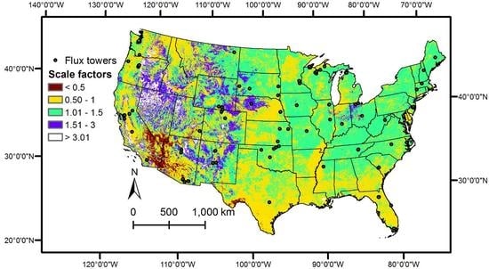
The scale factor map for creating the SSEBop-WB estimates is shown in Figure 7. This map was produced from the ratio of the long-term EWB ET (Figure 1a) to the long-term SSEBop ET (Figure 3a), except in locations of irrigation, where the scale factor map was given a value of 1 (original values are therefore unscaled). The individual monthly SSEBop ET maps were multiplied by this scale factor map to produce monthly SSEBop-WB estimates.
Comparisons using data from all available sites between the AmeriFlux data and the three methods are plotted in Figure 8. The R2 for the SSEBop-WB ET was highest, at 0.48 (RMSE = 39 mm/mo, bias = 2 mm/mo), followed closely by the SSEBop ET at 0.47 (RMSE = 38 mm/mo, bias = 0.4 mm/mo) and the MOD16 ET at 0.30 (RMSE = 39 mm/mo, bias = −6 mm/mo). Comparisons among the correlations showed that the MOD16 correlation was significantly different from the other two (p < 0.05), but that the correlations for SSEBop and SSEBop-WB were close enough not to be significantly different (p > 0.05).
The three methods were also compared with AmeriFlux data by month, to see whether different methods perform better depending on the time of year. The monthly and seasonal correlations are summarized in Table 1. The seasonal maps for the SSEBop-WB product are also shown in Figure 9. In general, all methods performed worse in winter months when ET magnitudes are lower. In the spring and summer, SSEBop-WB performed the best, while in the fall, SSEBop performed the best. In general, as there is less variation in ET over an individual month, overall R2 values are lower than for full year comparisons where there is a much broader spread in values. Though the individual monthly correlations were in general lower than the seasonal or total averages, all monthly correlations of all methods were statistically significant with p < 0.01.
In order to better understand method performance in different settings, we next split results by land cover type as identified in the 2006 National Land Cover Database. The results are summarized in Table 2. Such comparisons can help to guide users as to which data set may be more appropriate for a site with a given type of land cover. For example, although the MOD16 data set tended to underperform the others in most settings, it had the highest correlations in areas with land cover designated as “Barren”, “Forest”, or “Grass”.
4.4. Analysis of Residuals
The spatial distributions of the average residuals between the three method estimates and flux tower measurements are shown in Figure 10. These residual maps show which parts of the country are more accurately captured by which methods, and can be used to either refine the methods or to indicate locations where flux tower data may need reevaluation. For example, if a given method performed particularly poorly (with high residuals) in the southwest, the algorithm could be examined to see whether the modeling of ET in arid landscapes could be improved. Results are presented both for the magnitude of the residual (mm/mo, a–c), and for the residual normalized by the AmeriFlux value (d–f). Positive residuals indicate an overestimate of ET relative to the AmeriFlux towers.
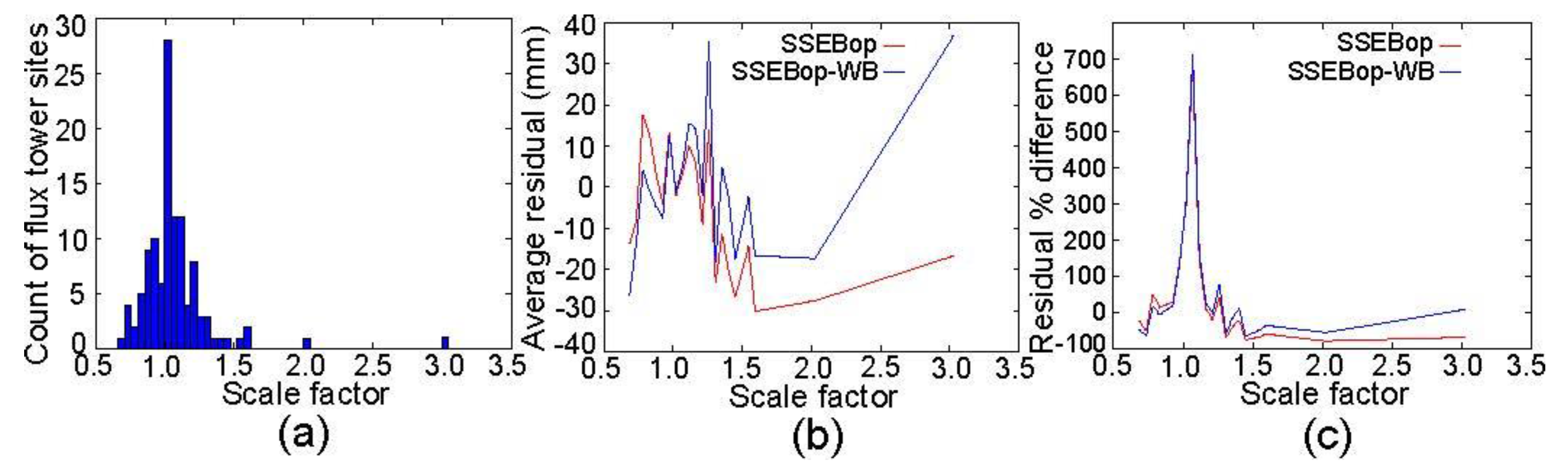
Though the SSEBop-WB shows an advantage in R2 when the complete data set is compared with the original SSEBop data (Figure 8), the improvement is not large, and individual months or land cover types can show advantages for either in certain settings (Table 1 and Table 2). The similar R2 values between SSEBop and SSEBop-WB are due partly to the method of SSEBop-WB development, where the temporal variation is entirely sourced from SSEBop but scaled by a constant scale factor for a given pixel location. The similarity is also due to the majority of flux towers being located where scale factors (Figure 7) are not far from 1, as can be seen in the histogram of Figure 11a. Binning and averaging the residual magnitude and percent difference by scale factor value, we compared the method performance as a function of scale factor value (Figure 11b–c). Spikes in the plots around a scale factor of 1.2 or 3 reflect individual outlier tower data points, but in general for scale factors higher than 1, the SSEBop-WB tended to show a smaller residual magnitude and percent difference than the SSEBop. For scale factors less than one, the residual magnitude for SSEBop tended to be positive while SSEBop-WB tended to be negative, and the percent difference was similar.
We also examined whether residuals of the three methods showed correlations with variables such as precipitation, temperature, and soil properties, as such correlations could indicate systematic biases in the algorithms that could be corrected. These results are summarized in Table 3. Most variables did not show a strong correlation with residuals of the three methods, with the possible exception of temperature variables, which showed correlations of 0.16–0.17 with SSEBop and SSEBop-WB. All correlations in Table 3 except those for soil available water capacity and soil thickness showed a statistical significance of p < 0.05.
Finally, as flux tower data sets are known to have uncertainties (see discussion in Section 3.2), we compiled a list of the sites that had the highest magnitude residuals with the three tested methods (Table 4) and the highest percent difference residuals (Table 5). Though these differences may be due to inaccuracies in the three remote sensing methods tested here, locations where all remote sensing methods show significant disagreements relative to the towers may also indicate errors within the flux tower data. Focused studies at these locations would be needed to determine whether the discrepancies at each were due to errors in either the remote sensing or flux tower measurements.
5. Discussion
We have presented here a new method and data set for combining remote sensing with long-term water-balance-based estimates for ET (see Acknowledgments for download information). The approach works to constrain non-irrigated remote sensing estimates to water-balance-based estimates for the purposes of (1) long-term magnitude accuracy; and (2) consistency with other water budget terms (e.g., not significantly exceeding precipitation); while (3) preserving the temporal frequency of measurements that remote sensing methods offer. To produce a combined monthly timescale ET data set, a scale factor map was created from the ratio of the long-term EWB ET to the long-term SSEBop ET. This scale factor map was applied to the monthly timescale SSEBop ET estimates, so that the modified SSEBop-WB estimates would equal the EWB ET estimates in the long-term average. An exception was made for the areas where irrigation was present in the MIrAD-US data sets, where the SSEBop estimates were confirmed to be more accurate and were left unscaled. This new data set of remote sensing-based ET estimates constrained by ground-based water balance data capitalizes on the advantages of both approaches.
The data were thoroughly tested and compared using 119 flux tower sites, with data processed for the monthly timescale. This study is unique from previous work partly because this is the most sites that have been used in such a comparison study evaluating remote sensing ET products by comparison with flux towers, compared to studies that have used a number of towers in the 45–85 range [9,16,11]. The unique collection of 5089 months of data from towers from many different settings, land cover types, and climate regimes across the country may have contributed to our overall R2 being lower than some previous studies, such as showing R2 = 0.64 for SSEBop [9], R2 = 0.80 for the Global Land Evaporation Amsterdam Model (GLEAM) ET product [11], or a skill score of 0.53 for MOD16 [12].
In our analysis, though the overall R2 for the new SSEBop-WB method was shown to be only slightly higher than the original SSEBop data when compared with the flux tower data, analysis of performance as a function of the scale factors at flux tower locations showed that the performance of the new method tends to provide a greater advantage at higher scale factor values, where the methods differ more significantly. The SSEBop-WB product has the additional benefit of consistency with other water budget components in the long term, without excessively exceeding long-term precipitation and irrigation water supply. The breakdowns of correlation by month, land cover type, and other variables will also be useful for deciding which method might be most appropriate for a given application. Though all the monthly timescale correlations were statistically significant, the R2 values for all methods were much lower for the monthly timescale than the overall R2, especially for the winter months. The use of the products at the monthly or seasonal timescale should consider the correlation levels in their use of the data sets. Though the comparison by land cover type more often showed a higher R2 for SSEBop-WB than SSEBop, the results are close and the RMSE for SSEBop were either equal to or slightly lower than the RMSE for SSEBop-WB. These comparisons by land cover type and time of year should help guide a user to which data set is more appropriate for an application; in some months and/or land cover types, particularly in applications where water balance constraints are not critical, the original SSEBop would be a better choice. In the overall comparison, and in most subsets of data comparison, the MOD16 data set showed the poorest correlations of the three methods tested. There were however a few specific months or land cover types for which MOD16 performed the best, so consideration of an appropriate product for a given application could indicate selection of MOD16.
Additional data sets were explored at the flux tower locations, such as irrigation presence, land cover, precipitation, temperature, soil properties, and impervious surface percent to explore the performance of SSEBop, MOD16, and the new SSEBop-WB method in different settings and at different times of year, and also to test for potential correlations with residuals between the remote sensing and flux tower measurements. Correlations with most variables tested were statistically significant, indicating that the method performances were systematically if subtly impacted by factors such as temperature, impervious surface percent, or precipitation rate. The temperature dependence showed the highest correlation with SSEBop and SSEBop-WB, where 16–17% of the variance of the increase in ET residual magnitude was explained by the value of the temperature. Such results could be used to inform future improvements in the algorithm treatment of temperature.
There has been some previous work to compare remote sensing-based estimates for ET with those from water-balance-based estimates [1,30], but none has previously worked to explicitly combine the two to capitalize on the complementary temporal frequency and magnitude accuracy advantages of each. The method presented here to combine the two approaches will provide a unique angle for future efforts to improve estimation of ET by incorporating all types of available data.
6. Conclusions
In this paper, a new data set has been produced and tested for the combination of ground-based water balance data with remote sensing ET data. The combination aims to combine the advantages of long-term magnitude accuracy and constraint within water budgets of the water-balance-based estimates with the remote sensing benefits of enabling shorter-timescale measuring of ET and improved accuracy in irrigated areas. By capitalizing on the complementary strengths of the two approaches, we have presented a method for scaling remote sensing ET products to water-balance constraints and produced a new SSEBop-WB ET data set for the monthly timescale. Such an approach could be followed to constrain other remote sensing ET products as well, particularly if/where their use is problematic due to errors related to exceeding water budget limitations. The new ET data set will be particularly appropriate for applications where water budget consistency is important, such as water balance hydrological models. Comparisons of the original SSEBop, the new SSEBop-WB, and the additional MOD16 data sets against data from 119 flux towers across the CONUS provided information about the performance of each method as a function of time of year, irrigation presence, and land cover type. The SSEBop-WB showed an improvement particularly in non-irrigated areas, where the SSEBop-WB R2 = 0.44, as compared to the SSEBop R2 = 0.41 or the MOD16 R2 = 0.36. The original SSEBop performed the best in the irrigated areas, and was left unscaled in those areas in the final SSEBop-WB product. Over all data points, the SSEBop-WB showed the highest overall R2 at 0.48, followed closely by SSEBop at 0.47 and then MOD16 at 0.30. For different land cover types of times of year, the method with the highest performance varied between the SSEBop-WB, SSEBop, and MOD16 data sets, and these results should be used to quantitatively guide users of these products to selection of an appropriate data set for a given application. The analysis of residuals by location in the country can help to inform checks on flux tower data accuracy as well as inform remote sensing method development and refinement. The SSEBop-WB maps are freely available for download [31], as is the scale factor map that could be used in conjunction with downloadable SSEBop data and the methods described here. The approach of scaling the magnitude of remote sensing ET estimates to converge to water balance-based data could also be taken in other regions outside the CONUS with sufficient water balance data. The new ET maps produced in this work will be useful for a variety of applications in water budget monitoring and water resource management.
Acknowledgments
We gratefully acknowledge the journal editor, three anonymous reviewers, and David Sumner for their constructive suggestions that helped improve the manuscript. AmeriFlux data are unpublished and provided free of charge. Funding for AmeriFlux data resources was provided by the U.S. Department of Energy’s Office of Science. The data produced in this paper are released in the USGS ScienceBase repository [31].
Author Contributions
Meredith Reitz, Ward E. Sanford and Gabriel B. Senay conceived and designed the study, and interpreted the results; Meredith Reitz carried out the analyses and wrote the paper; Ward E. Sanford and Gabriel B. Senay edited the paper.
Conflicts of Interest
The authors declare no conflict of interest.
References
- Reitz, M.; Sanford, W.E.; Senay, G.B.; Cazenas, J. Annual estimates of ET, recharge and quick-flow runoff for the contiguous US using empirical regression equations. J. Am. Water Resour. Assoc. 2017, 1–23. [Google Scholar] [CrossRef]
- Velpuri, N.M.; Senay, G.B. Partitioning Evapotranspiration into Green and Blue Water Sources in the Conterminous United States. Sci. Rep. 2017, 7, 6191. [Google Scholar] [CrossRef] [PubMed]
- Liou, Y.A.; Kar, S.K. Evapotranspiration estimation with remote sensing and various surface energy balance algorithms—A review. Energies 2014, 7, 2821–2849. [Google Scholar] [CrossRef]
- Roerink, G.J.; Bastiaanssen, W.G.M.; Chambouleyron, J.; Menenti, M. Relating crop water consumption to irrigation water supply by remote sensing. Water Resour. Manag. 1997, 11, 445–465. [Google Scholar] [CrossRef]
- Gilbert, J.M.; Maxwell, R.M. Examining regional groundwater-surface water dynamics using an integrated hydrologic model of the San Joaquin River basin. Hydrol. Earth Syst. Sci. 2017, 21, 923–947. [Google Scholar] [CrossRef]
- Olioso, A.; Chauki, H.; Courault, D.; Wigneron, J.P. Estimation of evapotranspiration and photosynthesis by assimilation of remote sensing data into SVAT models. Remote Sens. Environ. 1999, 68, 341–356. [Google Scholar] [CrossRef]
- Allen, R.G.; Tasumi, M.; Trezza, R. Satellite-based energy balance for mapping evapotranspiration with internalized calibration (METRIC)—Model. J. Irrig. Drain. Eng. 2007, 133, 380–394. [Google Scholar] [CrossRef]
- Bastiaanssen, W.G.M.; Menenti, M.; Feddes, R.A.; Holtslag, A.A.M. A remote sensing surface energy balance algorithm for land (SEBAL). 1. Formulation. J. Hydrol. 1998, 212, 198–212. [Google Scholar] [CrossRef]
- Senay, G.B.; Bohms, S.; Singh, R.K.; Gowda, P.H.; Velpuri, N.M.; Alemu, H.; Verdin, J.P. Operational evapotranspiration mapping using remote sensing and weather data sets: A new parameterization for the SSEB approach. J. Am. Water Resour. Assoc. 2013, 49, 577–591. [Google Scholar] [CrossRef]
- Olivera-Guerra, L.; Mattar, C.; Merlin, O.; Durán-Alarcón, C.; Santamaría-Artigas, A.; Fuster, R. An operational method for the disaggregation of land surface temperature to estimate actual evapotranspiration in the arid region of Chile. ISPRS J. Photogramm. Remote Sens. 2017, 128, 170–181. [Google Scholar] [CrossRef]
- Michel, D.; Jiménez, C.; Miralles, D.G.; Jung, M.; Hirschi, M.; Ershadi, A.; Martens, B.; McCabe, M.F.; Fisher, J.B.; Mu, Q.; et al. The WACMOS-ET project—Part 1: Tower-scale evaluation of four remote sensing-based evapotranspiration algorithms. Hydrol. Earth Syst. Sci. 2016, 20, 803–822. [Google Scholar] [CrossRef] [Green Version]
- Miralles, D.G.; Jiménez, C.; Jung, M.; Michel, D.; Ershadi, A.; McCabe, M.F.; Hirschi, M.; Martens, B.; Dolman, A.J.; Fisher, J.B.; et al. The WACMOS-ET project—Part 2: Evaluation of global terrestrial evaporation data sets. Hydrol. Earth Syst. Sci. 2016, 20, 823–842. [Google Scholar] [CrossRef] [Green Version]
- Mattar, C.; Franch, B.; Sobrino, J.A.; Corbari, C.; Jiménez-Muñoz, J.C.; Olivera-Guerra, L.; Skokovic, D.; Sória, G.; Oltra-Carriò, R.; Julien, Y.; et al. Impacts of the broadband albedo on actual evapotranspiration estimated by S-SEBI model over an agricultural area. Remote Sens. Environ. 2014, 147, 23–42. [Google Scholar] [CrossRef]
- “AmeriFlux: Measuring carbon, water and energy flux across the Americas.” Hosted by Lawrence Berkeley National Laboratory, U.S. Department of Energy. Available online: http://ameriflux.lbl.gov (accessed on 19 October 2017).
- Wilson, K.; Goldstein, A.; Falge, E.; Aubinet, M.; Baldocchi, D.; Berbigier, P.; Bernhofer, C.; Ceulemans, R.; Dolman, H.; Field, C.; et al. Energy balance closure at FLUXNET sites. Agric. For. Meteorol. 2002, 113, 223–243. [Google Scholar] [CrossRef]
- Mu, Q.; Zhao, M.; Running, S.W. Improvements to a MODIS global terrestrial evapotranspiration algorithm. Remote Sens. Environ. 2011, 115, 1781–1800. [Google Scholar] [CrossRef]
- Sanford, W.E.; Selnick, D.L. Estimation of Evapotranspiration across the Conterminous United States Using a Regression with Climate and Land-Cover Data. J. Am. Water Resour. Assoc. 2013, 49, 217–230. [Google Scholar] [CrossRef]
- Abatzoglou, J.T. Development of gridded surface meteorological data for ecological applications and modelling. Int. J. Climatol. 2013, 33, 121–131. [Google Scholar] [CrossRef]
- Daly, C.; Halbleib, M.; Smith, J.I.; Gibson, W.P.; Doggett, M.K.; Taylor, G.H.; Curtis, J.; Pasteris, P.P. Physiographically sensitive mapping of climatological temperature and precipitation across the conterminous United States. Int. J. Climatol. 2008, 28, 2031. Available online: prism.oregonstate.edu (accessed on 19 October 2017). [CrossRef]
- Hutson, S.S.; Barber, N.L.; Kenny, J.F.; Linsey, K.S.; Lumia, D.S.; Maupin, M.A. Estimated Use of Water in the United States in 2000; U.S. Geological Survey Circular; U.S. Geological Survey: Reston, VA, USA, 2004.
- Kenny, J.F.; Barber, N.L.; Hutson, S.S.; Linsey, K.S.; Lovelace, J.K.; Maupin, M.A. Estimated Use of Water in the United States in 2005; U.S. Geological Survey Circular; U.S. Geological Survey: Reston, VA, USA, 2009.
- Maupin, M.A.; Kenny, J.F.; Hutson, S.S.; Lovelace, J.K.; Barber, N.L.; Linsey, K.S. Estimated Use of Water in the United States in 2010; U.S. Geological Survey Circular; U.S. Geological Survey: Reston, VA, USA, 2014.
- Reitz, M.; Sanford, W.E.; Senay, G.B.; Cazenas, J. Annual estimates of recharge, quick-flow runoff, and ET for the contiguous US using empirical regression equations. J. Am. Water Resour. Assoc. 2017, 53, 961–983. [Google Scholar] [CrossRef]
- Allen, R.G.; Pereira, L.S.; Raes, D.; Smith, M. Crop Evapotranspiration—Guidelines for Computing Crop Water Requirements—FAO Irrigation and Drainage Paper 56; Food and Agriculture Organization of the United Nations (FAO): Rome, Italy, 1998. [Google Scholar]
- Van der Walt, S.; Colbert, S.C.; Varoquaux, G. The NumPy Array: A Structure for Efficient Numerical Computation. Comput. Sci. Eng. 2011, 13, 22–30. [Google Scholar] [CrossRef]
- Oliphant, T.E. Python for scientific computing. Comput. Sci. Eng. 2007, 9, 10–20. [Google Scholar] [CrossRef]
- Pervez, M.S.; Maxwell, S. Mapping irrigated lands across the United States using MODIS satellite imagery. In Remote Sensing of Global Croplands for Food Security; Thenkabail, P.S., Biradar, C.M., Turral, H., Lyon, J.G., Eds.; Taylor & Francis: Boca Raton, FL, USA, 2009; pp. 177–198. [Google Scholar]
- Fry, J.; Xian, G.; Jin, S.; Dewitz, J.; Homer, C.; Yang, L.; Barnes, C.; Herold, N.; Wickham, J. Completion of the 2006 National Land Cover Database for the Conterminous United States. Photogramm. Eng. Remote Sens. 2011, 77, 858–864. [Google Scholar]
- Soil Survey Staff, Natural Resources Conservation Service, United States Department of Agriculture. Web Soil Survey. Available online: http://websoilsurvey.nrcs.usda.gov/ (accessed on 19 October 2017).
- Velpuri, N.M.; Senay, G.B.; Singh, R.K.; Bohms, S.; Verdin, J.P. A comprehensive evaluation of two MODIS evapotranspiration products over the conterminous United States: Using point and gridded FLUXNET and water balance ET. Remote Sens. Environ. 2013, 139, 35–49. [Google Scholar] [CrossRef]
- Reitz, M.; Senay, G.B.; Sanford, W.E. Combined Remote Sensing and Water-Balance Evapotranspiration Estimates (SSEBop-WB) for the Conterminous United States. U.S. Geological Survey Data Release. 2017. Available online: https://doi.org/10.5066/F7QC02FK (accessed on 19 October 2017).
Figure 1.
(a) Map of annual average Empirical Water Balance (EWB) ET [1] across the conterminous U.S., for the 2000–2013 time period, from [1]; (b) Map of annual average ratio of ET to precipitation (ET/P) for the 2000–2013 time period. Here precipitation (P) from [1] includes input from groundwater-sourced irrigation. Values exceed 1 only in locations of open water.
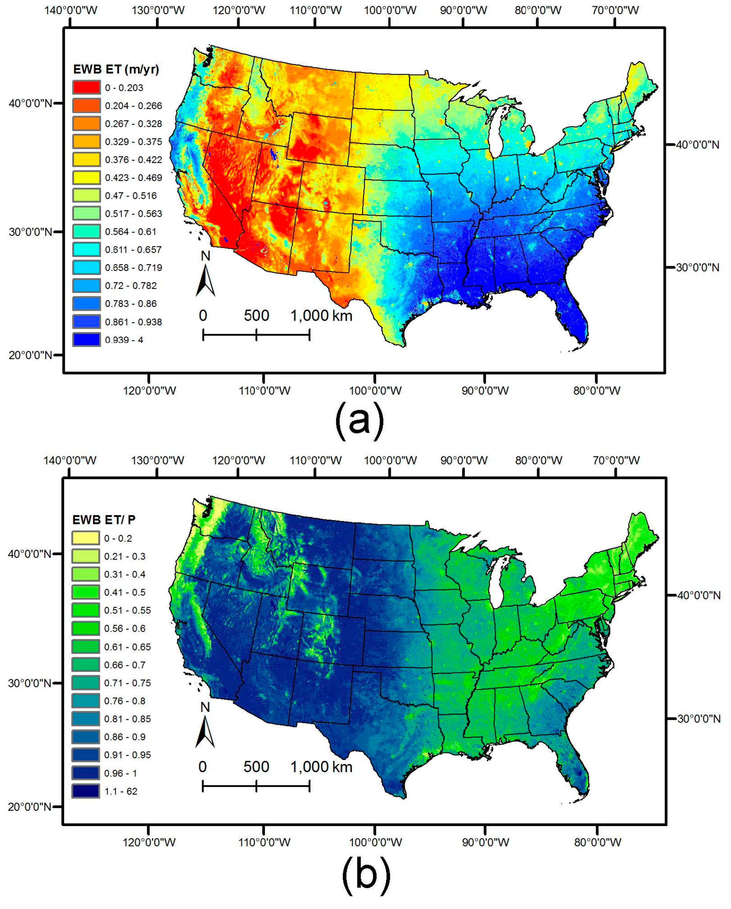
Figure 2.
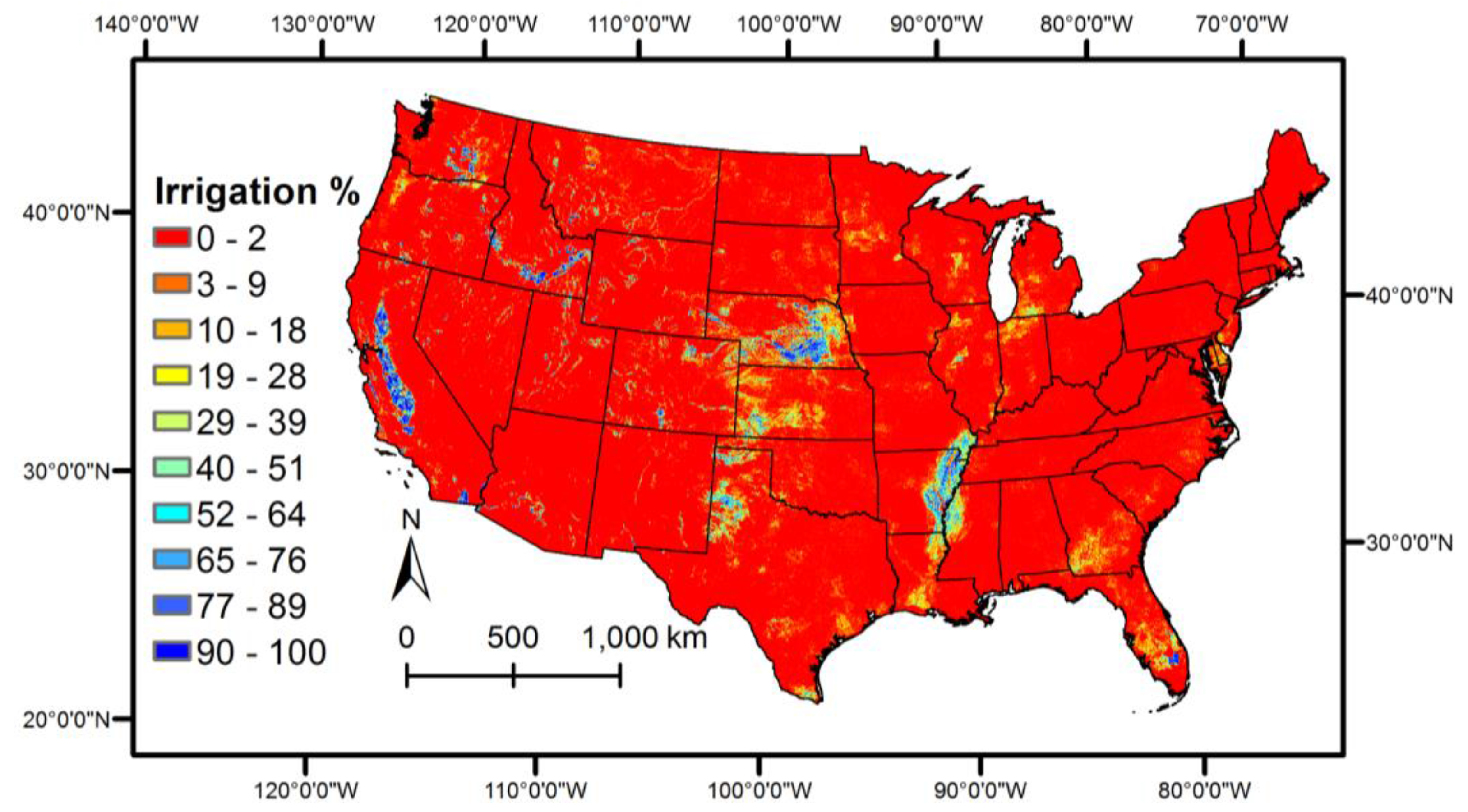
Map of irrigation intensity from the MODIS Irrigated Agriculture Datasets for the United States (MirAD-US), averaged over datasets from 2002, 2007, and 2012 [27].
Figure 2.
Map of irrigation intensity from the MODIS Irrigated Agriculture Datasets for the United States (MirAD-US), averaged over datasets from 2002, 2007, and 2012 [27].

Figure 3.
Operational Simplified Surface Energy Balance (SSEBop) ET data. (a) Average annual ET for the 2000–2013 timespan as estimated using the SSEBop model; (b) ET/P for the SSEBop ET.
Figure 3.
Operational Simplified Surface Energy Balance (SSEBop) ET data. (a) Average annual ET for the 2000–2013 timespan as estimated using the SSEBop model; (b) ET/P for the SSEBop ET.
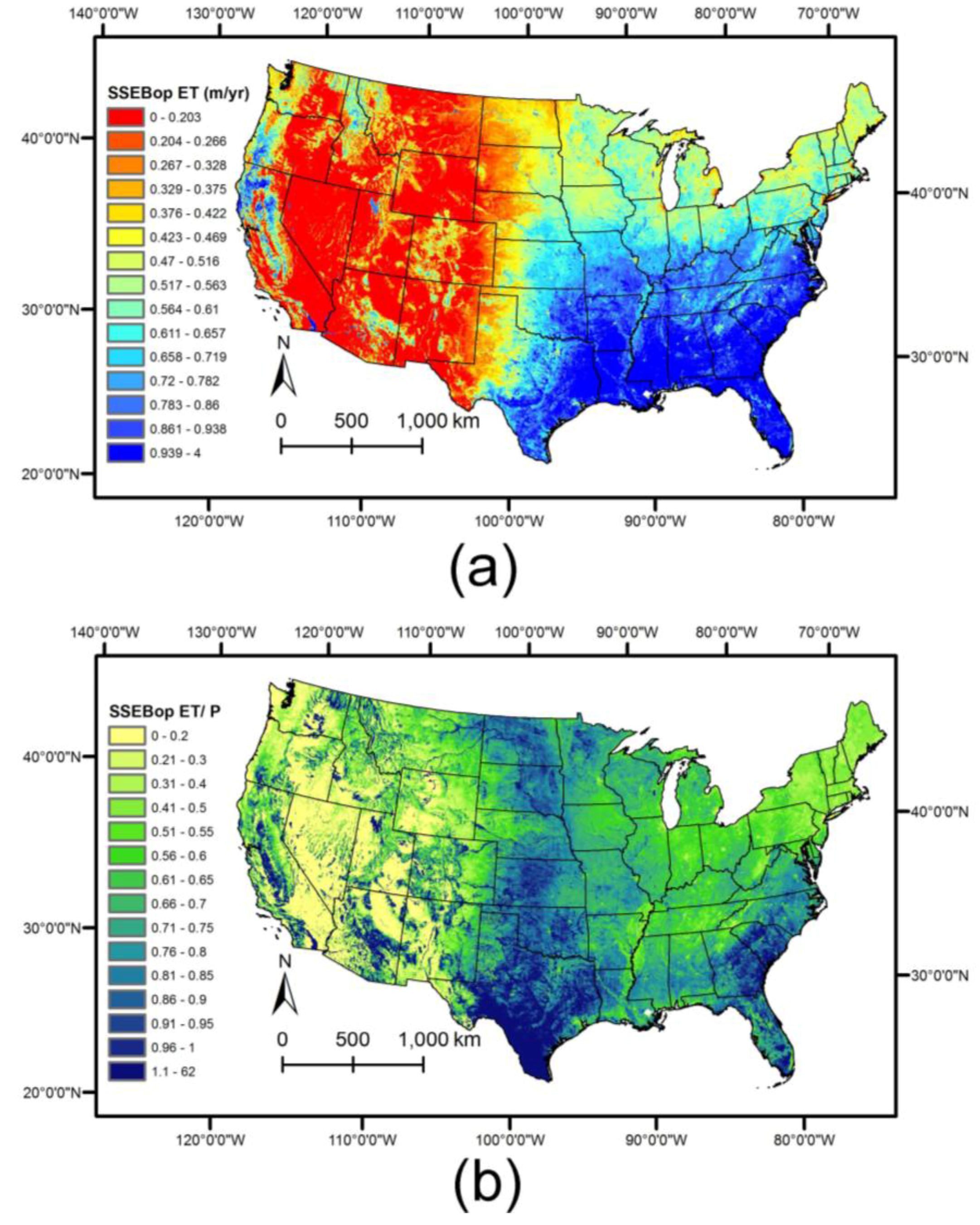
Figure 4.
MOD16 ET data. (a) Average annual ET for the 2000–2013 timespan as estimated using the MOD16 model; (b) ET/P for the MOD16 ET. Clear areas (no data) represent urban areas or water bodies, which are not included in MOD16 data sets.
Figure 4.
MOD16 ET data. (a) Average annual ET for the 2000–2013 timespan as estimated using the MOD16 model; (b) ET/P for the MOD16 ET. Clear areas (no data) represent urban areas or water bodies, which are not included in MOD16 data sets.
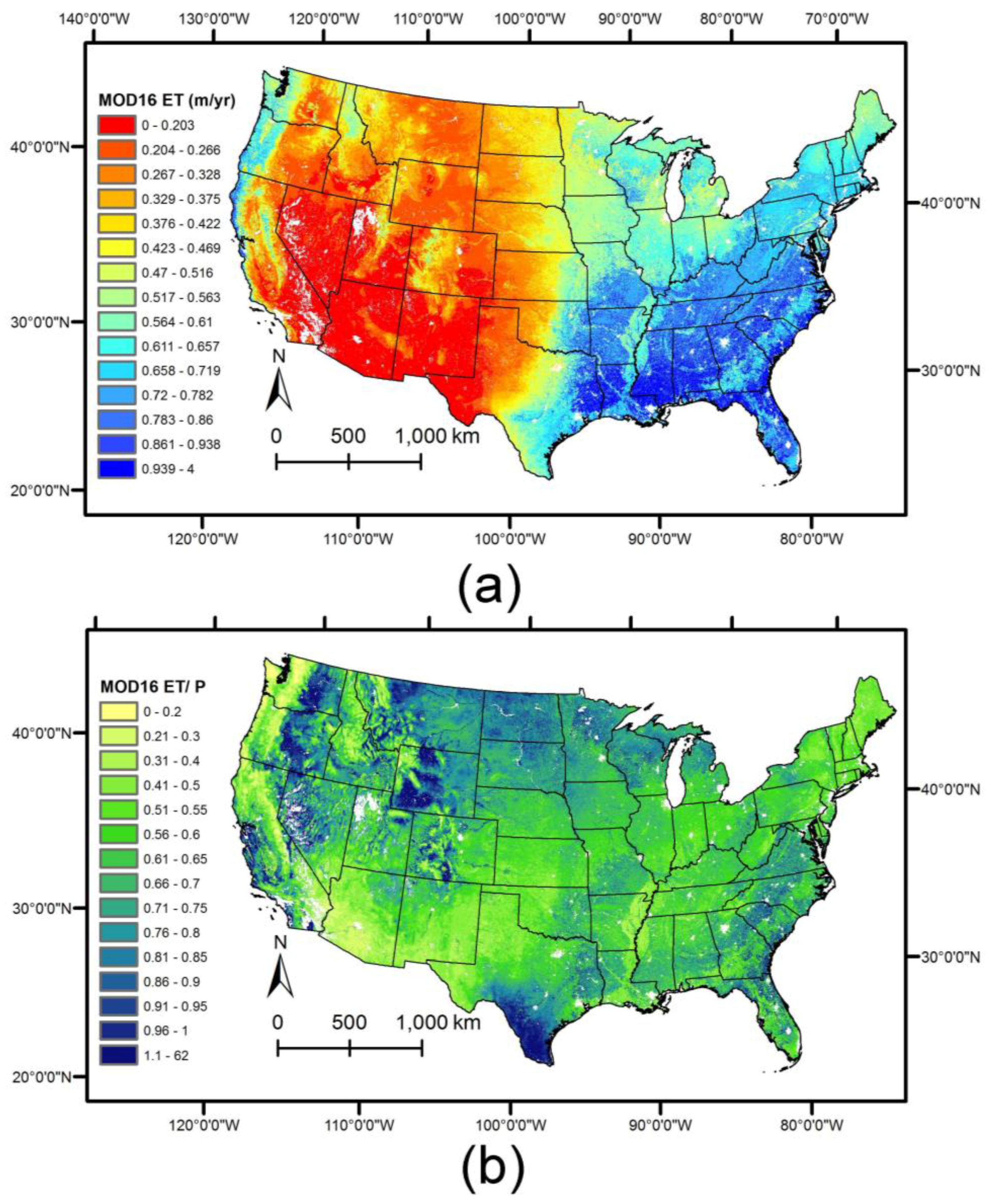
Figure 5.
Comparisons of AmeriFlux data with the ET predictions only in tower locations where the MIrAD-US product (Figure 2) indicated active irrigation, for (a) scaled SSEBop; (b) SSEBop; and (c) MOD16.
Figure 5.
Comparisons of AmeriFlux data with the ET predictions only in tower locations where the MIrAD-US product (Figure 2) indicated active irrigation, for (a) scaled SSEBop; (b) SSEBop; and (c) MOD16.
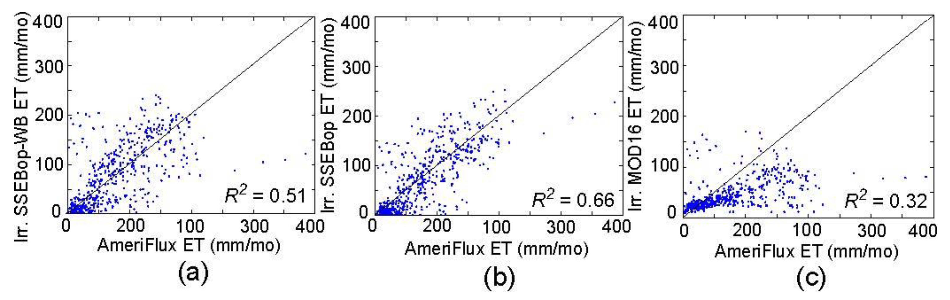
Figure 6.
Comparisons of AmeriFlux data with the ET predictions only in tower locations where the MIrAD-US product (Figure 2) did not indicate active irrigation, for (a) scaled SSEBop; (b) SSEBop; and (c) MOD16.
Figure 6.
Comparisons of AmeriFlux data with the ET predictions only in tower locations where the MIrAD-US product (Figure 2) did not indicate active irrigation, for (a) scaled SSEBop; (b) SSEBop; and (c) MOD16.
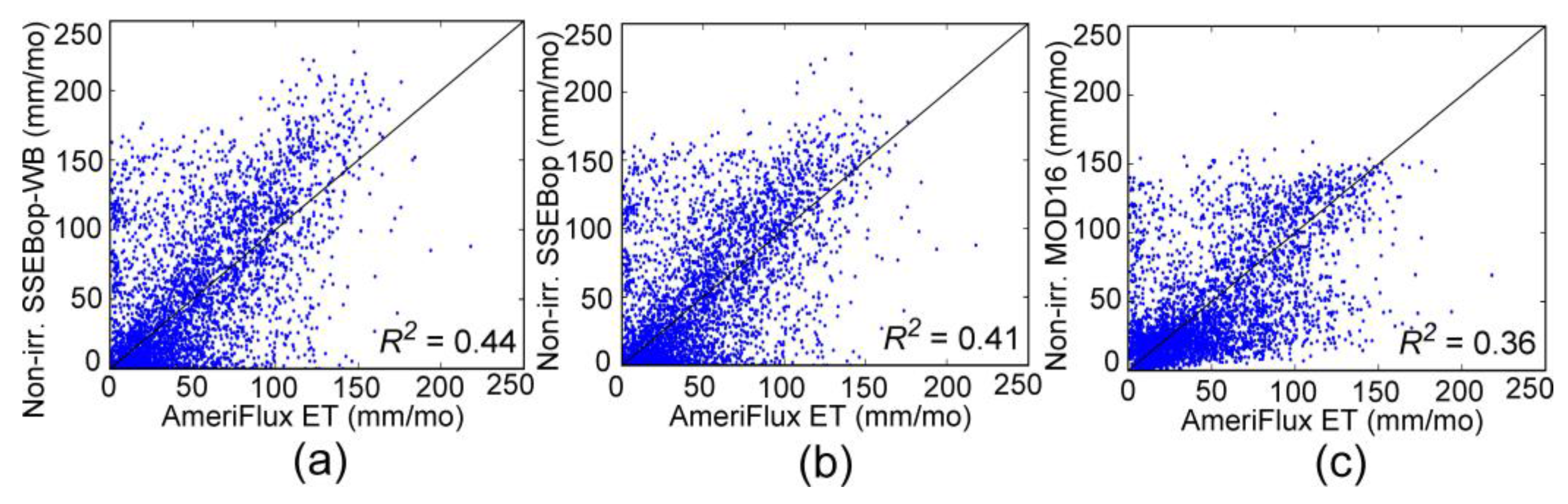
Figure 7.
Scale factor map used in converting SSEBop ET estimates to SSEBop/Water-Balance (SSEBop-WB) ET estimates. Locations of AmeriFlux towers are also shown. This map represents the ratio of the long-term EWB ET (Figure 1a) to the long-term SSEBop ET (Figure 3a), except in irrigated areas where the scale factor values are set to 1.
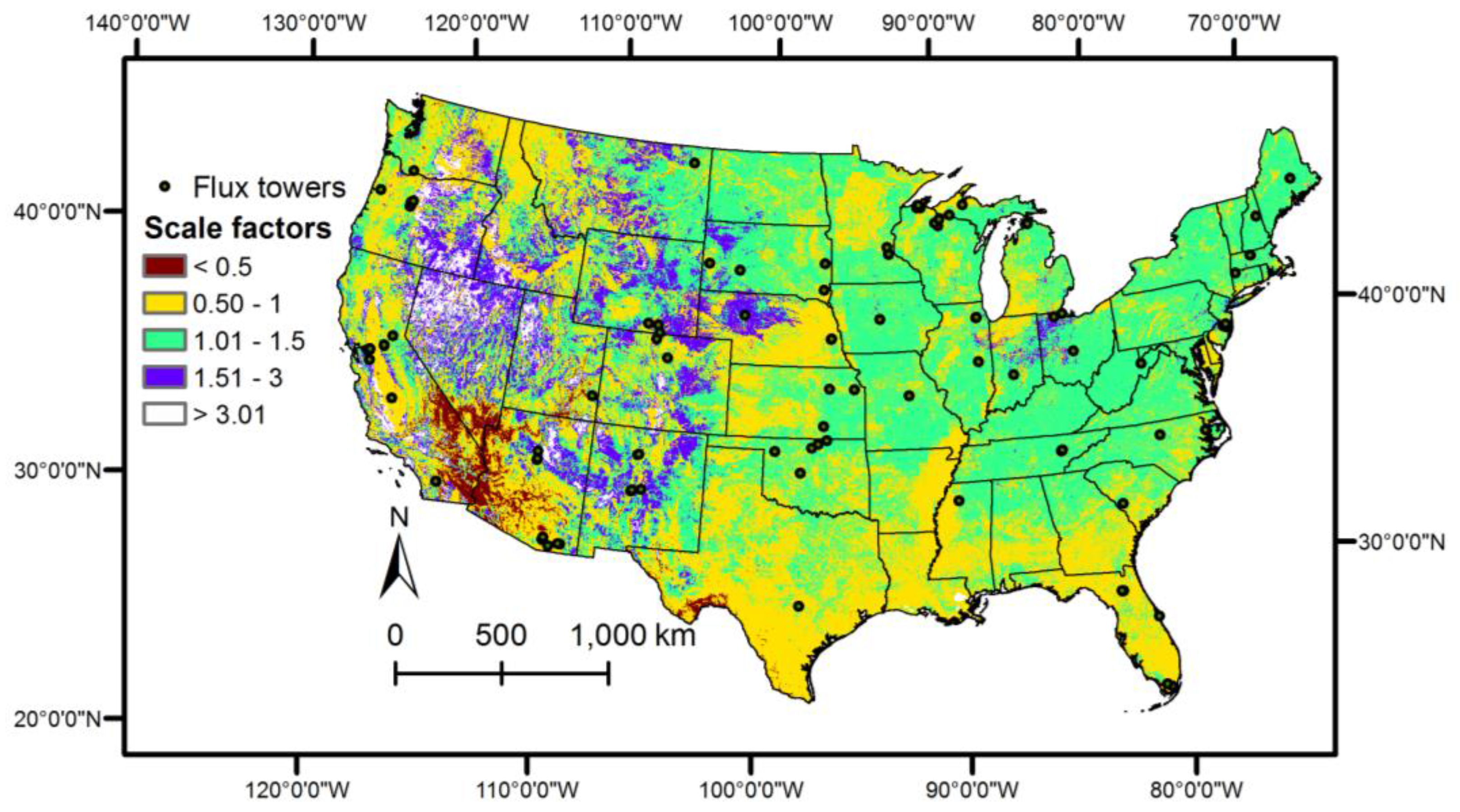
Figure 8.
AmeriFlux data comparison at monthly time scale. AmeriFlux ET data (x-axes) are compared with (a) SSEBop-WB ET; (b) SSEBop ET; and (c) MOD16 ET.
Figure 8.
AmeriFlux data comparison at monthly time scale. AmeriFlux ET data (x-axes) are compared with (a) SSEBop-WB ET; (b) SSEBop ET; and (c) MOD16 ET.
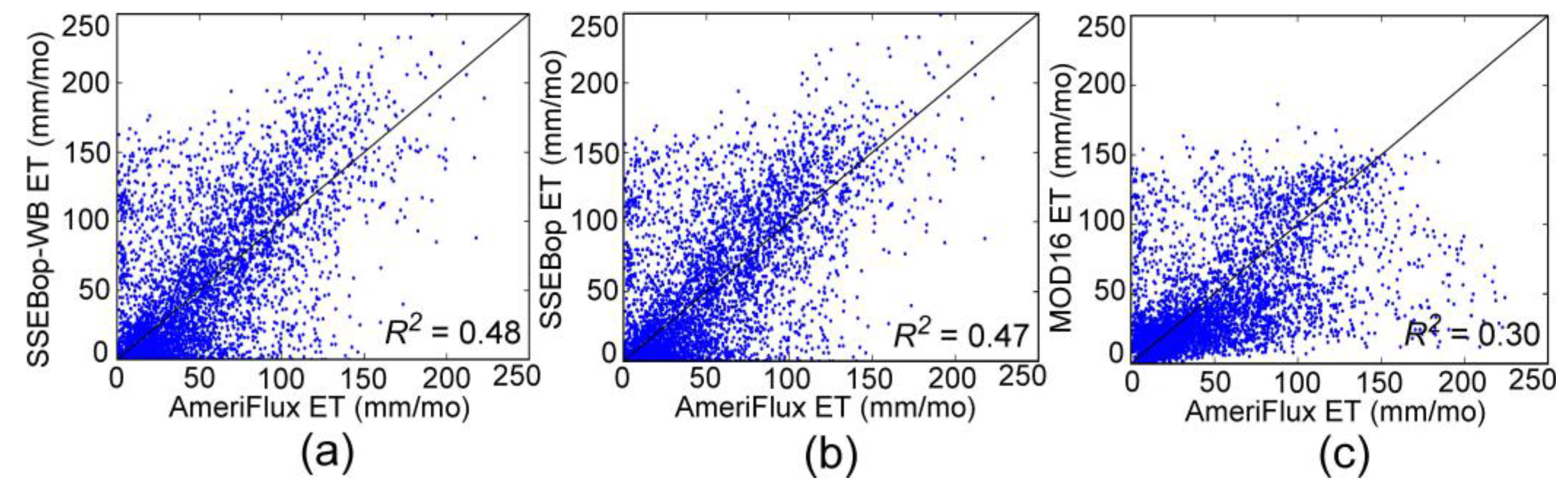
Figure 9.
Seasonal averages of the monthly SSEBop-WB data set, for the 2000–2015 time period: (a) Spring (March, April, May); (b) Summer (June, July, August); (c) Fall (September, October, November); and (d) Winter (December, January, February).
Figure 9.
Seasonal averages of the monthly SSEBop-WB data set, for the 2000–2015 time period: (a) Spring (March, April, May); (b) Summer (June, July, August); (c) Fall (September, October, November); and (d) Winter (December, January, February).
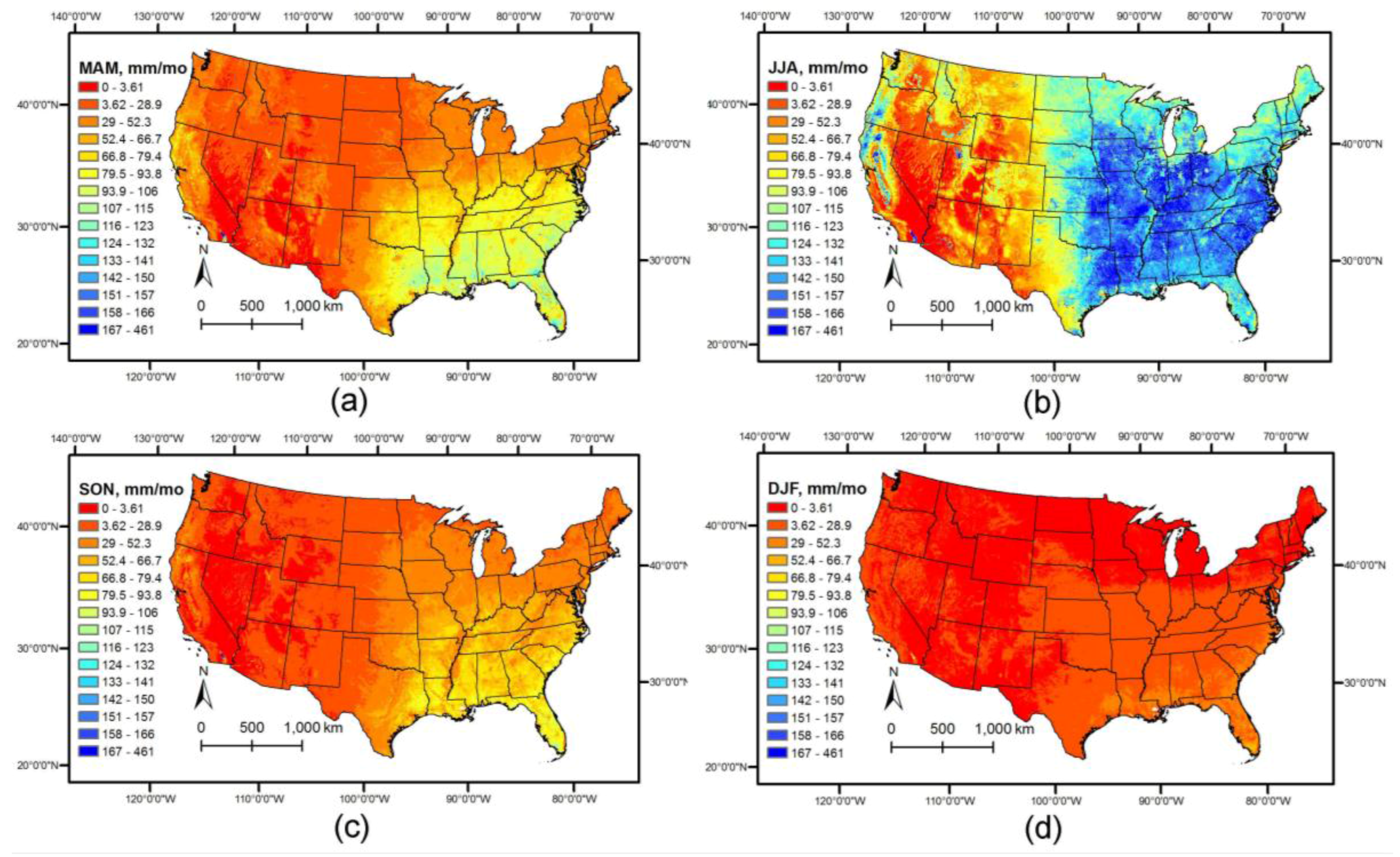
Figure 10.
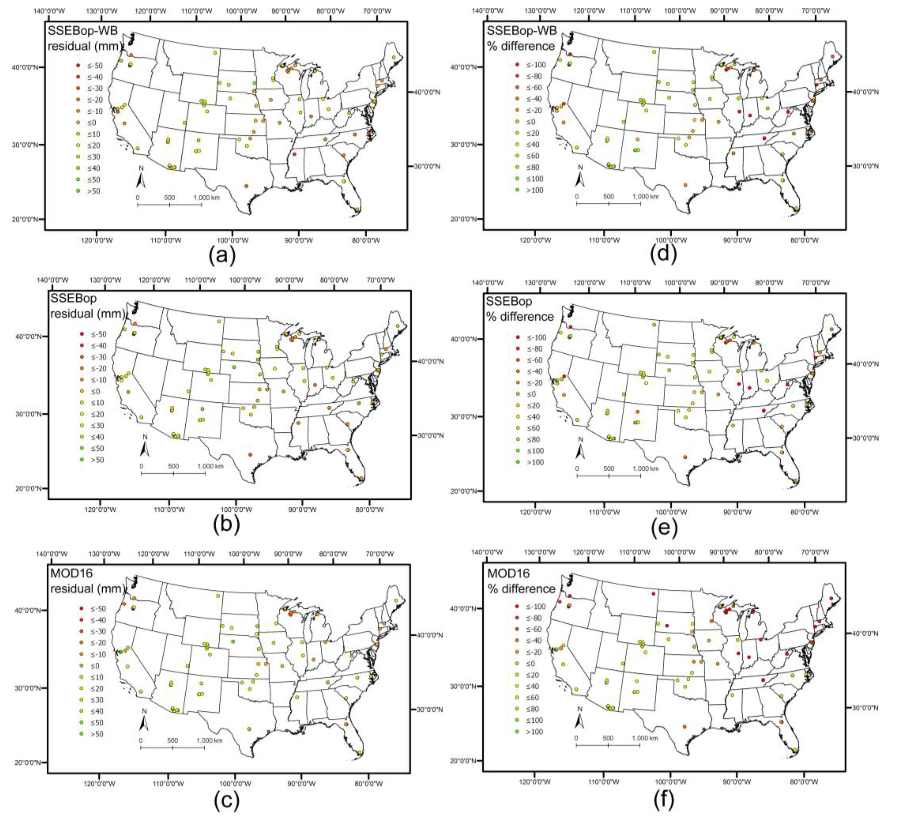
Residuals plotted as magnitudes of the average monthly difference between the three tested methods and the AmeriFlux tower data, for: (a) The SSEBop-WB ET; (b) The SSEBop ET; and (c) The MOD16 ET. The residuals are also plotted as percent differences between the three methods and the AmeriFlux tower data, for: (d) The SSEBop-WB ET; (e) The SSEBop ET; and (f) The MOD16 ET.
Figure 10.
Residuals plotted as magnitudes of the average monthly difference between the three tested methods and the AmeriFlux tower data, for: (a) The SSEBop-WB ET; (b) The SSEBop ET; and (c) The MOD16 ET. The residuals are also plotted as percent differences between the three methods and the AmeriFlux tower data, for: (d) The SSEBop-WB ET; (e) The SSEBop ET; and (f) The MOD16 ET.

Figure 11.
Comparison of SSEBop and SSEBop-WB relative to scale factor values at AmeriFlux sites. (a) Histogram of the distribution of scale factor values at flux tower sites; (b) Average magnitude of residuals for the tower measurements, relative to scale factor values; (c) Average percent difference between SSEBop or SSEBop-WB values and tower ET measurements, relative to scale factor values.


Table 1.
Correlations between AmeriFlux data and the three ET methods by month and season. All correlations are statistically significant with p < 0.01.
Table 1.
Correlations between AmeriFlux data and the three ET methods by month and season. All correlations are statistically significant with p < 0.01.
| Time Period | R2, SSEBop-WB | R2, SSEBop | R2, MOD16 | Number of Sites | Months of Data |
|---|---|---|---|---|---|
| January | 0.09 | 0.11 | 0.08 | 85 | 395 |
| February | 0.12 | 0.13 | 0.15 | 77 | 357 |
| March | 0.14 | 0.14 | 0.19 | 89 | 433 |
| April | 0.21 | 0.20 | 0.17 | 90 | 424 |
| May | 0.34 | 0.30 | 0.22 | 89 | 437 |
| June | 0.37 | 0.31 | 0.13 | 97 | 444 |
| July | 0.29 | 0.26 | 0.06 | 94 | 448 |
| August | 0.19 | 0.17 | 0.04 | 91 | 449 |
| September | 0.19 | 0.21 | 0.07 | 90 | 443 |
| October | 0.21 | 0.24 | 0.26 | 89 | 459 |
| November | 0.14 | 0.17 | 0.31 | 84 | 419 |
| December | 0.09 | 0.11 | 0.14 | 85 | 381 |
| Winter (DJF) | 0.10 | 0.12 | 0.12 | 92 | 1133 |
| Spring (MAM) | 0.34 | 0.32 | 0.26 | 99 | 1294 |
| Summer (JJA) | 0.29 | 0.26 | 0.08 | 100 | 1341 |
| Fall (SON) | 0.32 | 0.34 | 0.26 | 100 | 1321 |
| All | 0.48 | 0.47 | 0.30 | 119 | 5089 |
Table 2.
Monthly statistical metrics for the different methods by land cover type from the 2006 NLCD. The R2, RMSE, and bias of each method when compared with AmeriFlux data are listed for each land cover type.
Table 2.
Monthly statistical metrics for the different methods by land cover type from the 2006 NLCD. The R2, RMSE, and bias of each method when compared with AmeriFlux data are listed for each land cover type.
| Product | Metric | Agriculture | Urban | Barren | Forest | Shrubs | Grass | Marsh |
|---|---|---|---|---|---|---|---|---|
| SSEBop-WB | R2 | 0.513 | 0.834 | 0.426 | 0.322 | 0.55 | 0.584 | 0.505 |
| RMSE (m/mo) | 0.042 | 0.016 | 0.028 | 0.043 | 0.023 | 0.033 | 0.047 | |
| bias (m/mo) | 0.002 | 0.002 | 0.004 | 0.005 | −0.012 | 0.003 | 0.01 | |
| SSEBop | R2 | 0.513 | 0.834 | 0.423 | 0.324 | 0.572 | 0.575 | 0.496 |
| RMSE (m/mo) | 0.039 | 0.014 | 0.024 | 0.043 | 0.023 | 0.031 | 0.043 | |
| bias (m/mo) | −0.002 | −0.001 | −0.003 | 0.006 | −0.011 | 0.001 | 0.001 | |
| MOD16 | R2 | 0.155 | 0.81 | 0.51 | 0.328 | 0.398 | 0.62 | 0.235 |
| RMSE (m/mo) | 0.05 | 0.025 | 0.019 | 0.035 | 0.026 | 0.024 | 0.053 | |
| bias (m/mo) | −0.014 | 0.021 | −0.001 | 0.002 | −0.013 | −0.004 | −0.014 |
Table 3.
Correlations of residuals with other measured quantities at tower locations, to check for potential sources of systematic bias in the algorithms. All correlations except for soil available water capacity and soil thickness showed a statistical significance of p < 0.05.
Table 3.
Correlations of residuals with other measured quantities at tower locations, to check for potential sources of systematic bias in the algorithms. All correlations except for soil available water capacity and soil thickness showed a statistical significance of p < 0.05.
| Variable | R2, SSEBop-WB | R2, SSEBop | R2, MOD16 |
|---|---|---|---|
| Precipitation (mm/mo) | 0.013 | 0.014 | 0.004 |
| Temp max (°C) | 0.168 | 0.17 | 0.003 |
| Temp min (°C) | 0.163 | 0.172 | 0.002 |
| Temp mean (°C) | 0.169 | 0.174 | 0.002 |
| Temp range (°C) | 0.019 | 0.011 | 0.001 |
| Soil saturated hydraulic conductivity | 0.011 | 0.006 | 0.035 |
| Soil available water capacity | 0 | 0 | 0.01 |
| Soil field capacity | 0.005 | 0.001 | 0.049 |
| Soil porosity | 0.006 | 0.004 | 0.01 |
| Soil thickness | 0.003 | 0.004 | 0.002 |
| Percent impervious | 0.004 | 0.002 | 0.001 |
Table 4.
AmeriFlux sites with the highest average magnitude difference compared with remote sensing ET data sets, listed in descending order for the new SSEBop-WB data set, the SSEBop ET, and the MOD16 ET.
Table 4.
AmeriFlux sites with the highest average magnitude difference compared with remote sensing ET data sets, listed in descending order for the new SSEBop-WB data set, the SSEBop ET, and the MOD16 ET.
| Site ID | State | Latitude | Longitude | SSEBop-WB Residual (mm/mo) | SSEBop Residual (mm/mo) | MOD16 Residual (mm/mo) |
|---|---|---|---|---|---|---|
| US-Tw4 | CA | 38.103 | −121.641 | 25 | 25 | 118 |
| US-Myb | CA | 38.0498 | −121.765 | 23 | 23 | 114 |
| US-Tw1 | CA | 38.1074 | −121.647 | −3 | −3 | 154 |
| US-SdH | NE | 42.0693 | −101.407 | 29 | 51 | 61 |
| US-SP1 | FL | 29.7381 | −82.2188 | −29 | −40 | −44 |
| US-Bkg | SD | 44.3453 | −96.8362 | 32 | 32 | 36 |
| US-Wi7 | WI | 46.6491 | −91.0693 | −17 | −37 | −32 |
| US-Wi8 | WI | 46.7223 | −91.2524 | −12 | −27 | −37 |
| US-Los | WI | 46.0827 | −89.9792 | −28 | −21 | −26 |
| US-CPk | WY | 41.068 | −106.119 | 25 | 11 | 35 |
Table 5.
AmeriFlux sites with the highest average percent difference compared with remote sensing ET data sets, listed in descending order for the new SSEBop-WB data set, the SSEBop ET, and the MOD16 ET.
Table 5.
AmeriFlux sites with the highest average percent difference compared with remote sensing ET data sets, listed in descending order for the new SSEBop-WB data set, the SSEBop ET, and the MOD16 ET.
| Site ID | State | Latitude | Longitude | SSEBop-WB Residual Percent Diff. | SSEBop Residual Percent Diff. | MOD16 Residual Percent Diff. |
|---|---|---|---|---|---|---|
| US-Oho | OH | 41.5545 | −83.8438 | 71 | 74 | −164 |
| US-Ses | NM | 34.3349 | −106.744 | 93 | 92 | 70 |
| US-Los | WI | 46.0827 | −89.9792 | −89 | −66 | −80 |
| US-Seg | NM | 34.3623 | −106.702 | 73 | 77 | 58 |
| US-PFa | WI | 45.9459 | −90.2723 | −65 | −59 | −76 |
| US-Wrc | WA | 45.8205 | −121.952 | −83 | −75 | −38 |
| US-SP1 | FL | 29.7381 | −82.2188 | −48 | −66 | −73 |
| US-SRC | AZ | 31.9083 | −110.84 | 67 | 54 | 65 |
| US-Sta | WY | 41.3966 | −106.802 | 69 | 76 | 37 |
| US-LPH | MA | 42.5419 | −72.185 | −58 | −45 | −68 |
© 2017 by the U.S. Geological Survey (the work is in the public domain). Licensee MDPI, Basel, Switzerland. This article is an open access article distributed under the terms and conditions of the Creative Commons Attribution (CC BY) license (http://creativecommons.org/licenses/by/4.0/).
Share and Cite
MDPI and ACS Style
Reitz, M.; Senay, G.B.; Sanford, W.E. Combining Remote Sensing and Water-Balance Evapotranspiration Estimates for the Conterminous United States. Remote Sens. 2017, 9, 1181. https://doi.org/10.3390/rs9121181
AMA Style
Reitz M, Senay GB, Sanford WE. Combining Remote Sensing and Water-Balance Evapotranspiration Estimates for the Conterminous United States. Remote Sensing. 2017; 9(12):1181. https://doi.org/10.3390/rs9121181
Chicago/Turabian StyleReitz, Meredith, Gabriel B. Senay, and Ward E. Sanford. 2017. "Combining Remote Sensing and Water-Balance Evapotranspiration Estimates for the Conterminous United States" Remote Sensing 9, no. 12: 1181. https://doi.org/10.3390/rs9121181
Note that from the first issue of 2016, this journal uses article numbers instead of page numbers. See further details here.