New Scheme for Validating Remote-Sensing Land Surface Temperature Products with Station Observations


1
Chongqing Engineering Research Center for Remote Sensing Big Data Application, School of Geographical Sciences, Southwest University, No. 2 Tiansheng Road, Beibei District, Chongqing 400715, China
2
ICube, Uds, CNRS (UMR7357), 300 Bld Sebastien-Brant, CS10413, 67412 Illkirch, France
3
Heihe Remote Sensing Experimental Research Station, Northwest Institute of Eco-Environment and Resources, Chinese Academy of Sciences, 320 Donggang West Road, Lanzhou 730000, China
*
Authors to whom correspondence should be addressed.
Remote Sens. 2017, 9(12), 1210; https://doi.org/10.3390/rs9121210
Submission received: 27 September 2017
/
Revised: 10 November 2017
/
Accepted: 20 November 2017
/
Published: 24 November 2017
(This article belongs to the Special Issue Advances in Quantitative Remote Sensing in China – In Memory of Prof. Xiaowen Li)
Abstract
:Continuous land-surface temperature (LST) observations from ground-based stations are an important reference dataset for validating remote-sensing LST products. However, a lack of evaluations of the representativeness of station observations limits the reliability of validation results. In this study, a new practical validation scheme is presented for validating remote-sensing LST products that includes a key step: assessing the spatial representativeness of ground-based LST measurements. Three indicators, namely, the dominant land-cover type (DLCT), relative bias (RB), and average structure scale (ASS), are established to quantify the representative levels of station observations based on the land-cover type (LCT) and LST reference maps with high spatial resolution. We validated MODIS LSTs using station observations from the Heihe River Basin (HRB) in China. The spatial representative evaluation steps show that the representativeness of observations greatly differs among stations and varies with different vegetation growth and other factors. Large differences in the validation results occur when using different representative level observations, which indicates a large potential for large error during the traditional T-based validation scheme. Comparisons show that the new validation scheme greatly improves the reliability of LST product validation through high-level representative observations.
1. Introduction
Land-surface temperature (LST) is an important parameter related to the surface energy and water balance at local and global scales and has principal significance for applications such as monitoring the climate, hydrological cycle, and vegetation [1]. Satellite remote sensing provides a repetitive synoptic view in short intervals of the global land surface and is a vital tool for monitoring the LST of the Earth. With the development of remote-sensing technology, many LST products have been provided by different groups based on retrieval from different satellite data [2,3,4,5]. The first long-term global sensing LST dataset, the NOAA/NASA Pathfinder AVHRR Land dataset (PAL) [2], was released in 1994. The second generation AVHRR Land Pathfinder Π (PALΠ) was a refinement product from the PAL released in 2000 [3]. Sun and Pinker estimated LST products from a Geostationary Operational Environmental Satellite (GEOS) in 2003 [4]. The LSTs from Spinning Enhanced Visible and Infrared Imager (SEVIRI) onboard the Meteosat Second Generation (MSG) was retrieved in 2008 [6]. As a part of NASA Earth Observing System (EOS) project, MODIS LSTs have played an important role in recent studies, especially in regional studies, because of the suitable temporal and spatial resolution, acceptable accuracy, and accessibility of these LSTs. Therefore, MODIS daily LST/LSE products with 1-km spatial resolution are validated in this study.
Remotely sensed LSTs must be appropriately and precisely evaluated to ensure effective application [7]. Mainly two types of methods exist for validating LST products retrieved from thermal-infrared satellite data: temperature-based methods (T-based) and radiance-based methods (R-based) [8,9,10,11,12,13,14]. The main advantage of R-based methods is that they work during both the daytime and nighttime because in situ LST observations are not required, and finding validation sites with small spatial variations in land-surface emissivity is relatively easy [14]. However, the atmospheric and water vapor profiles at validation sites from radiosonde balloons that are synchronously launched with the satellite are a necessary dataset, which limits the implementation of this method for long-term and large-region validation. Therefore, T-based methods remain common, and ground-based measurements are still the primary source of datasets to directly validate remotely sensed LSTs. However, we cannot perform a direct comparison with a pixel grid, especially for a coarse-resolution product over heterogeneous areas, because of the spatial heterogeneity and different scales between ground-based observations and remotely sensed LST pixels.
A generally accepted method is a systematic site-to-network method, which deeply develops an in situ sampling strategy and upscaling approaches to acquire the truth at the pixel scale over a heterogeneous surface based on multiscale, multi-platform and multi-source observations [15]. This approach employs both field measurements from nodes of a wireless sensor network (WSN) and high-resolution remote-sensing data from synchronous high-resolution satellites or airborne sensors to establish a site-specific relationship and generate high-resolution LST reference maps over the validation area [15]. These LST reference maps are then treated as benchmarks to obtain multiscale validation datasets by upscaling methods [16,17,18]. However, only a few high-resolution LST reference maps can be synchronously obtained for a given region because of cost limitations and the revisiting cycles of satellites with high resolution, which is the greatest challenge towards the global validation of LST products, especially in terms of temporal consistency in product validation.
In contrast to more complicated R-based, site-to-network methods with limited LST reference maps, simple T-based methods are directly based on existing global, long-term ground LST measurements and are an important supplement for validation. Simple T-based methods have been widely used to validate remotely sensed LST products at homogeneous stations [8,13,19]. When directly validating LST products with spatial resolutions above hundreds or even thousands of meters by ground-based measurements, the error from the scale mismatch changes with the land-cover type (LCT) and the proportions of mixtures in pixel grids reduce the reliability of the validation and hinder the application of ground-based LST measurements during the validation of remotely sensed LST products. Coll et al. have pointed out that during the day, LST can vary by 10 K or more over a few meters in a heterogeneous surface [9]. Ground-based LST measurements from two types LST observation instruments with different field of view (FOV) were selected to discuss the scale mismatch implications for validation of remote sensing LST products in the study by Yu et al., and the validation results show that there is an extra 26.9% in the error >3 K range caused by the 41.5 FOV difference [20].Therefore, we must assess the spatial representativeness of station observations at a given spatial resolution to reliably validate remotely sensed LSTs. Recently, several methods have been used to assess the spatial representativeness of different land-surface parameters, such as the leaf area index [21], surface solar radiation [22], bidirectional reflectance distribution function (BRDF)/albedo [23], air temperature [24] and air quality [25], which are observed by ground stations. These methods are based on two factors: the point-to-area consistency and the spatial heterogeneity [21]. The point-to-area consistency indicator can be calculated through two methods. The first involves directly comparing the footprint of the ground-station observations to the corresponding product pixels [26] or the average value of the corresponding area [27]. In the second approach, the observational representativeness is determined by the average difference between a given station and its neighboring stations based on multi-temporal observations from multiple stations [9,28]. The semi-variance is usually selected to describe the spatial representativeness by analyzing the spatial heterogeneity around the stations [29]. A first-order statistical algorithm is an important spatial heterogeneity indicator, for example, using window-size analysis to assess the spatial variation of the landscape around a given station [30]. Spatial representativeness assessments have been widely implemented to validate satellite-albedo, evapotranspiration, and LAI products [21,23,26,31,32]. However, few representativeness assessments exist for station LST observations, which increases the uncertainty of the validation of LST products, particularly for simple T-based implementations, and hinders the application of station observations.
This paper presents a new methodology for validating LST products that focuses on quantifying the spatial representativeness of station observations to improve the accuracy and reliability of LST product validation. The term “spatial representativeness” refers to measurements of the degree to which ground-based observations can resolve the surrounding LST by extending to the satellite footprint. This validation technique assesses the spatial characteristics of the LST, and the seasonal representativeness changes within a statistical framework. A scheme that is based on spatial representativeness indicators is presented in this paper, and then the grading criteria are outlined in detail. All the stations from the Heihe Watershed Allied Telemetry Experimental Research (HiWATER) [33] are selected for applying the validation strategy. The study area and data-processing procedure are introduced in Section 3. In Section 4, the representativeness of the given station observations is assessed to validate MODIS V5 daily LST products (MOD/MYD11A1). The representativeness assessment and LST product validation are also analyzed and discussed in this Section. Finally, the conclusions are summarized.
2. Methodology
2.1. New Validation Scheme
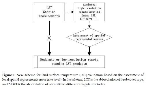
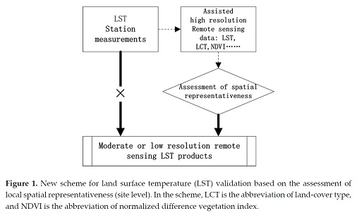
The LST is a land-surface parameter with great spatial and temporal heterogeneity, which creates many challenges for “point-to-pixel” comparisons. Local changes in the surface temperature within and between different ecosystems introduce scale mismatch errors. Moreover, these patterns change seasonally and are particularly difficult to identify during periods of rapidly changing surface conditions. Therefore, “point” measurements alone are not sufficient to validate satellite-derived LST retrievals, especially remote-sensing LST products with moderate and low resolution (illustrated in Figure 1). This temporal mismatch can be solved by increasing the observation-acquisition frequency of stations. The scheme that is developed here to validate remote-sensing LST products (see Figure 1) attempts to solve spatial mismatch effects during validation. The key in this scheme is to assess the spatial representativeness, which is based on remote-sensing data with high spatial resolution that are closely related to the LST. Indicators are proposed to quantify the spatial representativeness, and then the grading criteria are designed before selecting appropriate ground-based measurements for validation.
2.2. Indicators for Assessing Spatial Representativeness
Three indicators are proposed to describe the spatial characteristics for a specific parameter, mainly including the consistency from points to pixels and the spatial heterogeneity within pixels. These indicators are calculated on high-resolution images, which are much easier to access, thus simplifying the process. The LST is a direct parameter for assessing the representativeness of a given station’s LST observations. However, obtaining temporal high-spatial-resolution LST matches for LST products with lower resolution is difficult. Therefore, high-resolution land-cover type (LCT) and the normalized difference vegetation index (NDVI), which can indicate the surface conditions and their changes, are chosen as additional supporting parameters to evaluate ground-based LST observations in addition to LST data with a high spatial resolution.
If the LCTs observed by stations do not match the dominant LCTs in the pixels, these station LST observations cannot represent the LST of the LCTs in the pixels. Thus, the dominant LCT (DLCT), which is given by the percentage of the observed LCT throughout the pixel’s area, is defined as
where is the product pixel, is the area with the LCT that is observed by the given station, and is the total area of the LCTs in the LST product’s pixel grid. When using a high-resolution LCT map, the DLCT can also be described as the percentage of fine pixel numbers covered by station-observed LTC to total LCT pixel numbers in the LST product’s pixel range. A high DLCT indicates that the LCT observed by a station is consistent with that in the LST product’s pixel and low heterogeneity within the product pixel because the mixing rate of LCTs in the pixel is not large.
We developed a relative bias (RB) indicator to assess how close a ground-based LST measurement is to the value of the corresponding pixel area. According to the high-spatial-resolution LST reference images, the relative bias is used to describe the difference between the LST value at a station and the average LST value in the product pixel’s area. If we consider the comparability between different ranges of LST values, the RB is defined as
where s is the product pixel and RB depends on both its resolution and the resolution of the reference LST image. This indicator can quantify the certainty of the ground-based measurements to the product pixel area LST values. A smaller RB indicates more spatially representative observations for the corresponding pixel at the specific spatial resolution of s.
The two above indicators mainly measure the point-to-area value consistency, so the heterogeneity of the spatial distribution of the LST within a pixel, which is correlated with the vegetation growth, must be seasonally quantified. In terms of the spatial autocorrelation of LST parameters, semivariogram is one of the most commonly used and efficient geostatistical analysis tools for quantitatively evaluating spatial variations. Semi-variance and related geostatistical kriging were developed from mining research during the late 1950s and have been widely used after a publication by Journel and Huijbregts in 1978 [34,35]. These geostatistical techniques have been used in many scientific projects, such as in describing the distribution and density of plants and animals [36,37] and in determining the spatial scales of variation and sampling strategies in remote sensing [38,39,40]. In regionalized variable theory, the semi-variance measures the dissimilarity of a spatial variable observed at different locations. The semi-variance is calculated by the average squared difference between observations and , which are separated by distance , as described below:
where is the number of observation pairs, which are separated by a distance , or lag, as intervals to calculate the semi-variance. In this study, the variogram estimator is computed on discretized point values from high-spatial resolution LST pixels, and then a variogram model is established as a parametric functional approximation based on these semi-variance values. Several theoretical variogram model types exist, including linear models, spherical models, exponential models, and Gaussian models. Among these models, spherical models are the most widely used variogram models for their strong fitting and generalization capabilities and are recommended for assessing the spatial representativeness of observations [23,32]. The isotropic spherical variogram that is used to estimate the variogram is as follows:
In Equation (4), it is obvious that the generally increases from a nonzero value to a relatively stable constant value with . When , the value is a nonzero value , namely, , and is the nugget of the variogram. The stable constant value is the sill of the variogram. When reaches the sill, the value of the variable is a, namely, the range of the variogram. The key parameters range (), nugget (), and sill can be obtained from fitting Equation (4). is the maximal distance between the two correlated points and indicates the average structural scale (ASS) of the given area. The nugget indicates the level of ’s randomness, which may be caused by internal variations in over a smaller distance than the sampling distance or may be derived from the sampling error. The sill represents the largest extent of the regionalized variation. Li and Reynolds [41] introduced the proportion of structural variation, which is based on subtracting the variogram nugget () from the sill () and then dividing by the sill, to discuss the definition and quantification of ecological heterogeneity. However, the heterogeneity of LST parameters considerably varies over time when compared to that of ecological parameters, and reference high-resolution LST maps may not be completely synchronous with the validated LST products. Therefore, the ASS is introduced based on the range of the variogram model, which reflects the average structural scale of the given area and the size of the homogeneous area. A large ASS value indicates that the station observations represent a large homogeneous area.
3. Data Instruction and Preparation
3.1. Ground-Based LST Measurements
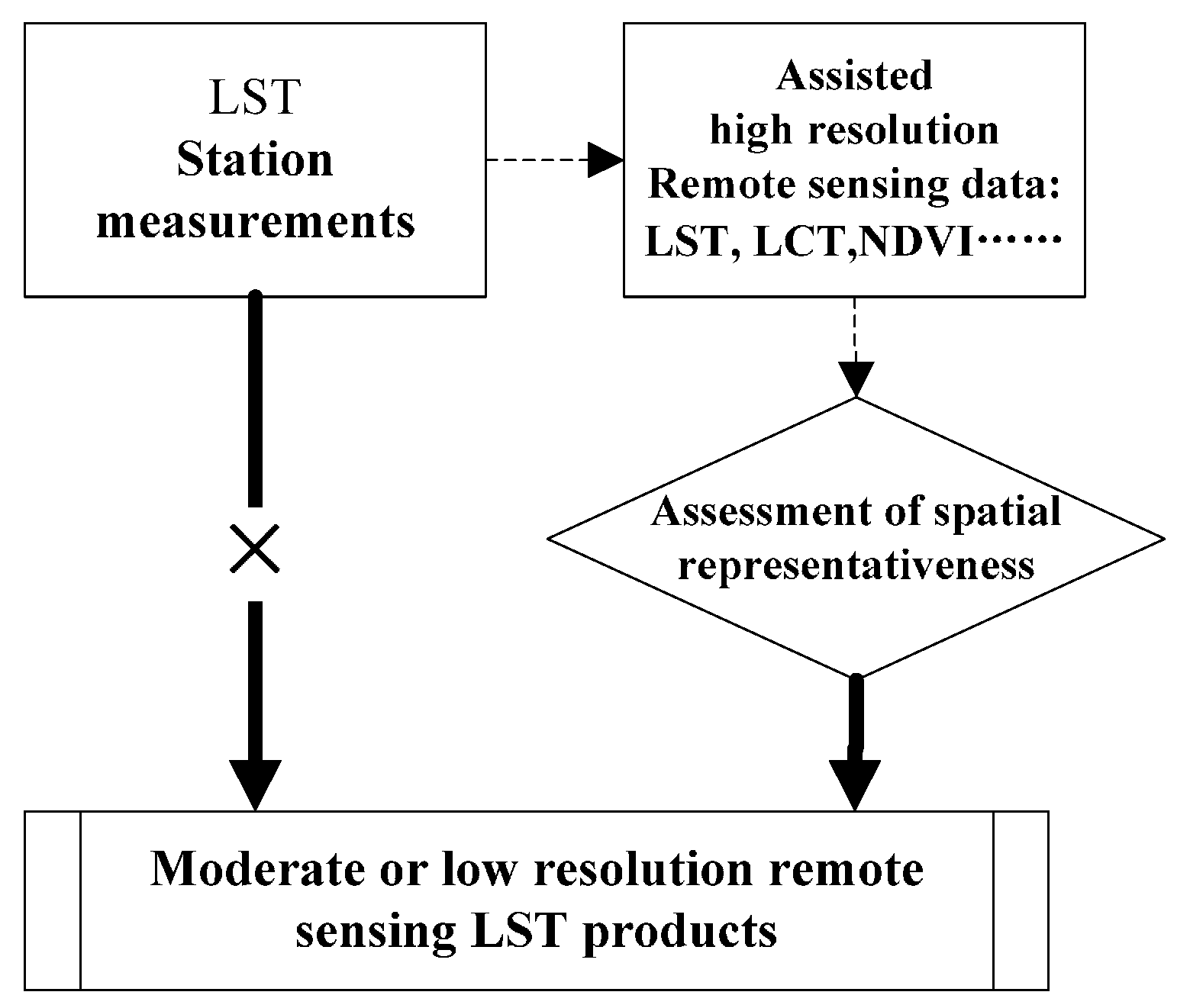
In this study, we selected the Heihe River Basin (HRB), which is the second largest inland valley in China’s arid regions, to evaluate MODIS LSTs with 1-km resolution. The HRB is located in the northern arid region within 97.1°E–102.0°E and 37.7°N–42.7°N. Glaciers, frozen soils, alpine meadows, forests, irrigated crops, riparian ecosystems, deserts, and gobi are distributed from upstream to downstream regions (see Figure 2). The HRB was selected as an experimental watershed to reveal the processes and mechanisms of the ecohydrological system in an inland river basin. Allied telemetry experiments such as the Heihe Basin Field Experiment (HEIFE) [42] and Watershed Allied Telemetry Experimental Research (WATER) [43] have been conducted in the HRB, and the HiWATER [33] project has been ongoing since 2012. The stations that collect watershed hydrological observations cover a wider range than those in previous studies and provide a large amount of ecohydrological data for evaluation. Eighteen atmospheric stations from HiWATER are scattered around the HRB region. Longwave-radiation data for eighteen stations from 2013 to 2014 were selected to obtain ground-based LSTs to evaluate the MODIS LSTs. The locations of the stations are shown in Figure 2. The information for the stations is listed in Table 1, and environmental photos of these sites are shown in Figure 3. The ARC, ARS, ARY, DSL, JYL, HZS, HCG, and EBZ stations are located in the upstream area; the DMZ, GBZ, HZZ, SDZ, and SSW stations are located in the midstream area; and the downstream area contains the SDQ, HJL, HYZ, NTZ, and LTZ stations. The LCTs of these stations are all typical types in the three significantly different areas.
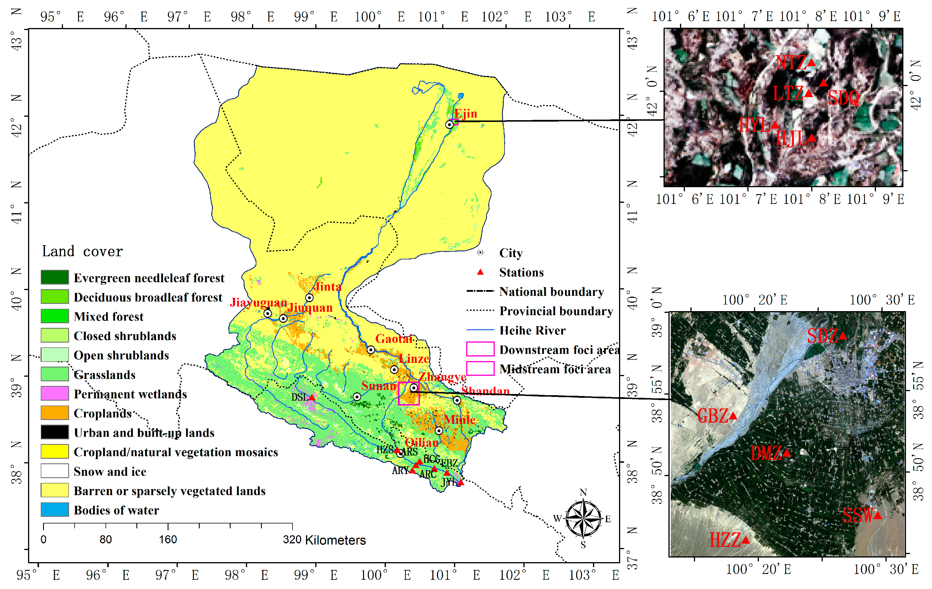
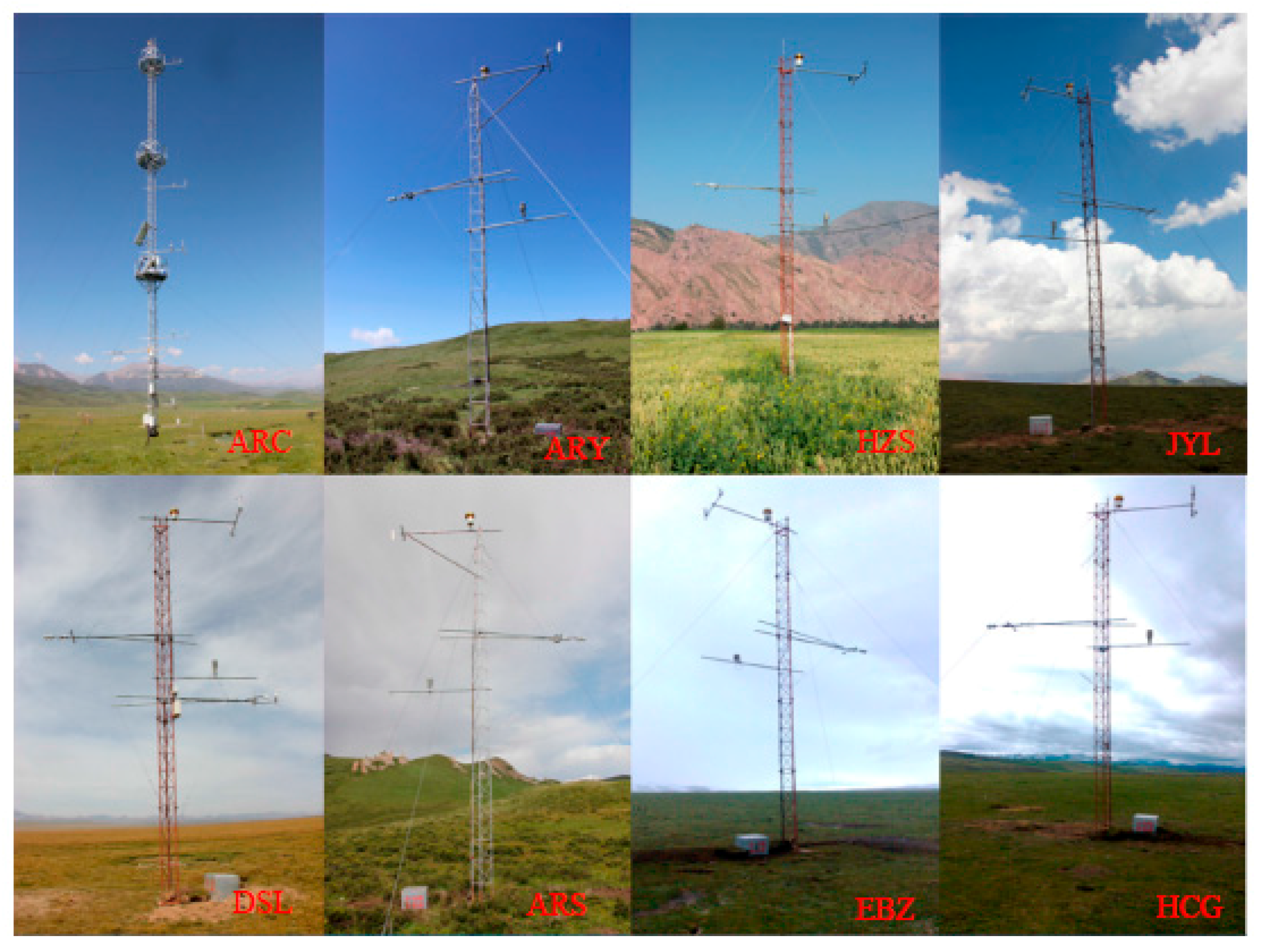
Eighteen meteorological towers are located in the HRB region, consisting of three superstations and fifteen ordinary stations. Pyrgeometers are deployed at these 10-m to 35-m high meteorological station towers to measure longwave radiation (see Figure 3 and Table 1). At least two pyrgeometers are positioned on a single tower: one facing upward and the other facing downward. The field-of-view (FOV) of the upward-facing pyrgeometer is nearly 180°, while that of the downward-facing pyrgeometer is 150°. Therefore, the effective diameter of the FOV of the pyrgeometers on a 10-m to 35-m tower is approximately 2.5–24 m with a 6-m average mounting height, and the diameters of the ground-observation footprints are shown in Table 1. The pyrgeometers are sensitive to the spectral range from 4.5 to 42 µm in the longwave band. All the instruments at each station were calibrated before and after field deployment. Field-routing exams were implemented once per month. Assurance and quality control provided the best possible data for the level-2 daily data. All these data and related information can be found at the HiWATER website [44]. All the ground-based measured data from the eighteen HiWATER sites were 10-min averaged values. The longwave radiation data were selected according to the field viewing time for the MODIS LST. The LST is related to land-surface longwave radiation according to the Stefan-Boltzmann law [1,45]:
where is the surface upwelling longwave radiation, is the surface broadband emissivity, is Stefan-Boltzmann’s constant (5.67 × 10⁻⁸ W∙m−2∙K−4), and is the atmospheric downwelling longwave radiation at the surface. Therefore, the ground-measured LST can be estimated from station longwave-radiation observations by the following equation:
In Equation (6), and are obtained from the ground-based measurements. Seven narrowband emissivities exist in MOD/MYD11B1 LST/LSE products. can be estimated from these MODIS narrowband emissivities [45]:
where is the broadband emissivity, and , , and are the narrow emissivity products of MODIS bands 29, 31, and 32 that are retrieved from the MODIS day/night LST algorithm (MOD/MYD11B1 LST/LSE).
3.2. Remote-Sensing Data
3.2.1. MODIS Data
As a component of NASA’s Earth Observing System (EOS) project, two MODIS instruments were placed onboard the Terra and Aqua satellite platforms to provide information for global atmosphere-, land- and oceanic-process studies [46]. MOD/MYD22_L2, MOD/MYD11A1, MOD/MYD11B1 and MOD/MYD07_L2 are all daily LST products based on thermal-infrared data from MODIS. MOD/MYD11_L2 was retrieved by a generalized split-window algorithm with 1-km spatial resolution [47]. MOD/MYD11A1 is tile-based and gridded in the sinusoidal projection from MOD/MYD11_L2. MOD/MYD11B1 was obtained using the day/night LST algorithm at 5-km spatial resolution [48]. MOD/MYD07_L2 was retrieved by the atmospheric team using statistical regression methods [49]. In this study, we focus on the collection of 5 MOD/MYD11A1 products, which are more widespread. Uncertainties from the satellite measurements and improvements in the original MODIS LSTs for cloudy days are beyond the scope of this paper. To eliminate effects from the inversion algorithm and clouds, only pixels with high-quality MODIS LSTs were selected for the evaluation based on a quality control flag value of 0. The narrow emissivity products from MOD/MYD11B1 LST/LSE were selected to estimate the land-surface broadband emissivity and obtain ground-based LSTs [45]. The narrow emissivities from MOD/MYD11B1 LST/LSE at 5-km resolution were resampled to 1-km spatial resolution to match the evaluated MODIS LSTs.
3.2.2. High-Spatial-Resolution Images
Land-cover images with a spatial resolution of 30 m (data doi:10.3972/hiwater.155.2014.db, downloaded from the HiWATER land cover datasets [50], which were produced by Zhong et al. [51,52], were selected to obtain the DLCT in a 1-km LST product pixel. This dataset was mainly based on charge-coupled device (CCD) data from the Huan Jing 1 (HJ-1) satellite, which was launched on 6 September 2008, by the China Center for Resources Satellite Data and Application (CRESDA). HJ-1/CCD has three visible bands and one near-infrared band [53]. This dataset provides monthly land-cover maps of the HRB from 2011 to 2015 with 30-m spatial resolution. LCTs change with the seasons, and these changes are similar across consecutive years, so the DLCT products in 2013 were collected to calculate the DLCT indicator.
Landsat 8, which is called the Landsat Data Continuity Mission, is extending the distinguished 40-year records of Landsat-series satellites and has enhanced capabilities, such as adding new spectral bands in the visible and thermal-infrared wavelengths and improving the signal-to-noise ratio and radiometric resolution of the sensor [54]. The Landsat 8 satellite includes two instruments: an Operational Land Imager (OLI) and Thermal Infrared Sensor (TIRS). High-resolution LST maps were retrieved from the Landsat 8 TIRS data and OLI data. Before retrieving the LST maps, the Landsat OLI and TIRS images were preprocessed, including radiometric calibration and atmospheric correction based on the correction model in the ENVI software. Monthly NDVI maps were obtained to assess the relationships between the monthly changes in the indicators and vegetation growth. The NDVI maps were based on the visible red band (R, band 4) and the near-infrared band (NIR, band 5) according to the following equation:
In this study, the LST data were estimated from the TIRS aboard Landsat 8 based on a practical split-window (SW) algorithm developed by Du et al. [55]. The SW algorithm can be expressed as follows:
where is LST, and are the TOA brightness temperatures in the thermal-infrared channels and , respectively; is the average emissivity of the two channels (i.e., ); is the channel emissivity difference (i.e., ); and are the algorithm coefficients from the simulated dataset. In this algorithm, the coefficients were determined based on atmospheric water-vapor subranges, which were obtained through a modified split-window covariance-variance ratio method. The channel emissivities were acquired from newly released global land-cover products at 30 m and a fraction of the calculated vegetation cover from visible and near-infrared images that were obtained by Landsat 8.
The effect of heterogeneity changes depending on the season, so we selected Landsat 8 data from September 2013 to August 2014 with a 16-day temporal resolution to calculate the RB, and ASS. A total of 92 Landsat 8 images for all the stations in the HRB were downloaded from the following USGS website [56]. The statistical results were based on per-month averages to eliminate invalid data from cloud cover.
4. Results and Discussion
4.1. Spatial Representativeness Classification
Since the DLCT and RB can measure point-to-pixel value consistency, and ASS can assess the spatial patterns for a given station, respectively. Therefore, all three indicators were combined to describe the representativeness including point-to-pixel consistency and spatial heterogeneity. The spatial representativeness was also classified based on these three indicators. The DLCT indicator determines the representativeness of the station’s LCT in the product pixel. When the LCT in the view footprint of a station is not dominant within the product pixel, the station observations cannot be representative of the pixel, and the LST value of all other vegetation-cover types may be ignored, even if the point-to-area LST consistency is high at the station sometime. When a pixel has a large DLCT value, the RB and ASS subsequently would determine the spatial representativeness together. Presumably, the station-observed LSTs represent ideal data for LST product validation if the RB value is small and the ASS value is large. If the RB and are ASS value are both small, the station may have some spatial representation. In some extreme cases, the station observing area is an average heterogeneity sub-areas in the products pixel, which means the station observations are representative for pixels, although the surface is heterogeneous in these products pixels. Finally, if the RB is large but the ASS is small, the observations probably differ from the values of the pixel.
Reasonable thresholds for the DLCT, RB and ASS are required to determine the representativeness level of a given station’s observations. The emissivity products of the version 5 collection of MODIS LST/LSE products are retrieved based on the LCT of a pixel, and the LCT is classified as the land cover of this pixel based on the classification rule for MODIS land-cover products (MCD12Q1) if the area percent of one LCT in a pixel is higher than 60% [57]. Thus, 60% was defined as the threshold of the DLCT in this study. The RB was used to evaluate the difference between the land-based measurements within the view footprint at each station (in Table 1, the view footprints are shown in the sixth column) and the mean pixel value at the station locations. The ideal RB value is close to zero. However, the threshold of the RB is not unique and depends on the spatial resolution of the LST products, the view footprint of the station measurements, and the retrieval accuracy of the high-spatial-resolution LST maps that are used to evaluate the representativeness. Thus, a reasonable threshold for the RB was 0.5% in this study for MODIS LST products with 1-km spatial resolution, a station view footprint above 30 m and a 1-K retrieval error from the high-resolution LST map itself [55]. The ASS is calculated from variogram models based on the semi-variance in a 3-km × 3-km area that is centered at a given station and can indicate the greatest distance over which the value at a point on the surface is related to the value at another point. The ASS defines the maximum neighborhood over which control points should be selected to estimate a grid node to take advantage of the statistical correlation among observations and can describe the spatial distribution of LSTs and quantify the average LST spatial structures in the given area. In this study, the measurements from stations were used to evaluate the MODIS LSTs with a 1-km spatial resolution. Therefore, a reasonable ASS indicator should be larger than the spatial resolution of the LST products, that is, 1 km in this study.
The spatial representativeness of the station’s LST observations was classified into five different levels based on the difference-constraining degrees of the three indicators and their thresholds. The levels and their descriptions are presented in Table 2.
4.2. Representativeness Grading of the HiWATER Station Observations
The representativeness of the LST observations for the eighteen HiWATER stations was graded based on the three indicators and level in Table 2. Figure 4 shows the DLCT indicator results for the stations, and the red dashed line shows the threshold value of the DLCT in the figure. In the upstream area, all the stations were covered by grass or meadows, except for HZS, which was covered by wheat. The DLCT values within a 1-km pixel indicated that five stations were covered by a single LCT and one station (DSL) was covered by a dominant grass type, with a DLCT value above 80%. In the upstream area of the HRB, only one station (HZS) had a DLCT value below 60%. Among the five stations in the midstream area of the HRB, SSW, HZZ, and GBZ were covered by a single LCT and SDZ was dominated by one type within a 1-km pixel. The LCTs within a 1-km pixel were diverse and broken at DMZ, and the DLCT value of the station observations was less than 60%. The LCTs of the five downstream stations were more complex within a 1-km pixel, and their DLCT values were all less than 60%. According to the DLCT threshold, the observations of seven stations, including HZS, DMZ, SDQ, HJL, HYL, NTZ, and LTZ, were graded at Level 5 (Table 2). Eleven remaining stations exhibited vegetation-type cover, matching the types in the corresponding MODIS LST pixels, but their representative levels varied depending on the RB and ASS values.
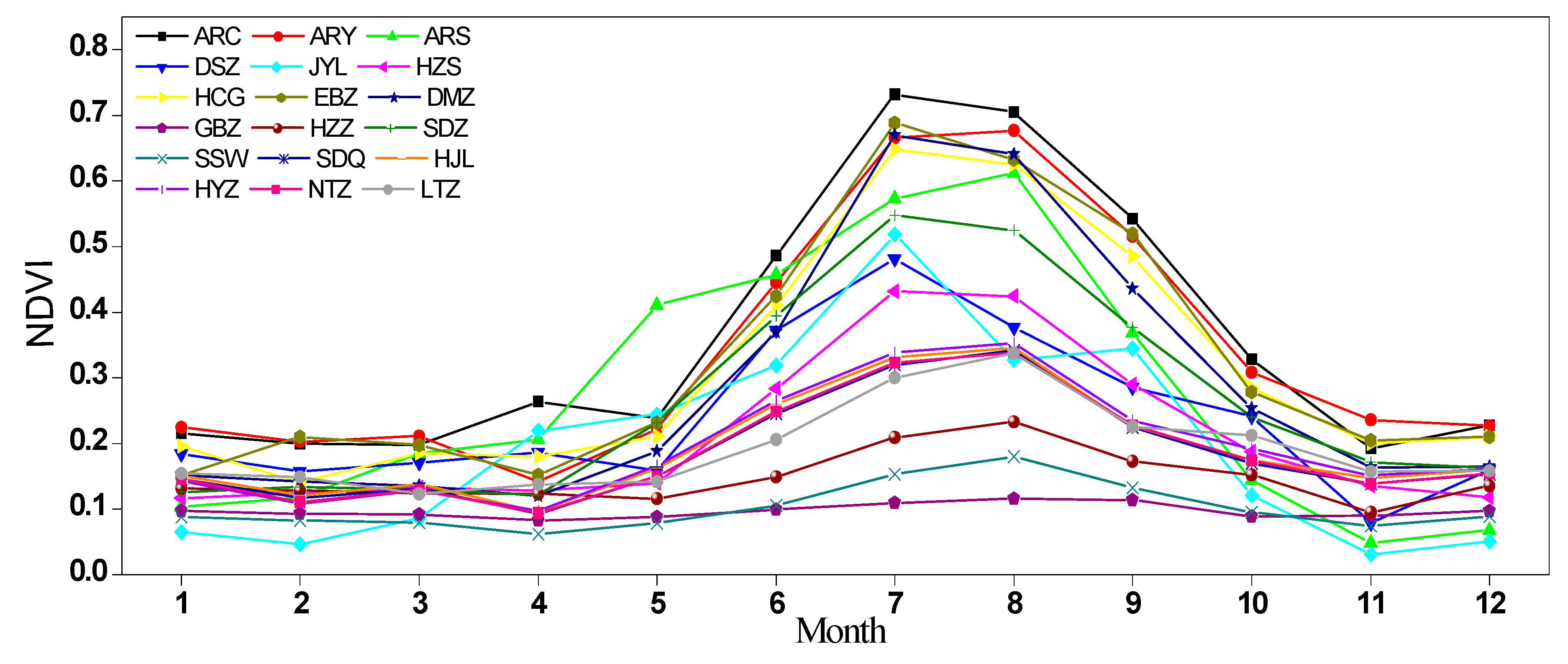
The annual vegetation growth at stations can severely affect changes in their spatial representativeness. When stations have homogeneous vegetation types and density, the representativeness of stations may not vary with vegetation growth. Instead, the representativeness changes with the level of the point-to-area LST match, vegetation-density homogeneity and spatial contexture of the pixel during different seasons. The spatial representativeness of station observations can vary with vegetation growth in a year. When the vegetation type is uniform and the density is homogeneous, the representativeness at different growth stages may not significantly change. Otherwise, the representativeness may change because of changes in the point-to-area consistency and spatial heterogeneity. Seasonal changes in the spatial representativeness are similar in consecutive years when not interfered with by outside influences. Therefore, the RB and ASS values of the station observations were calculated monthly and are shown in Figure 5 and Figure 6.
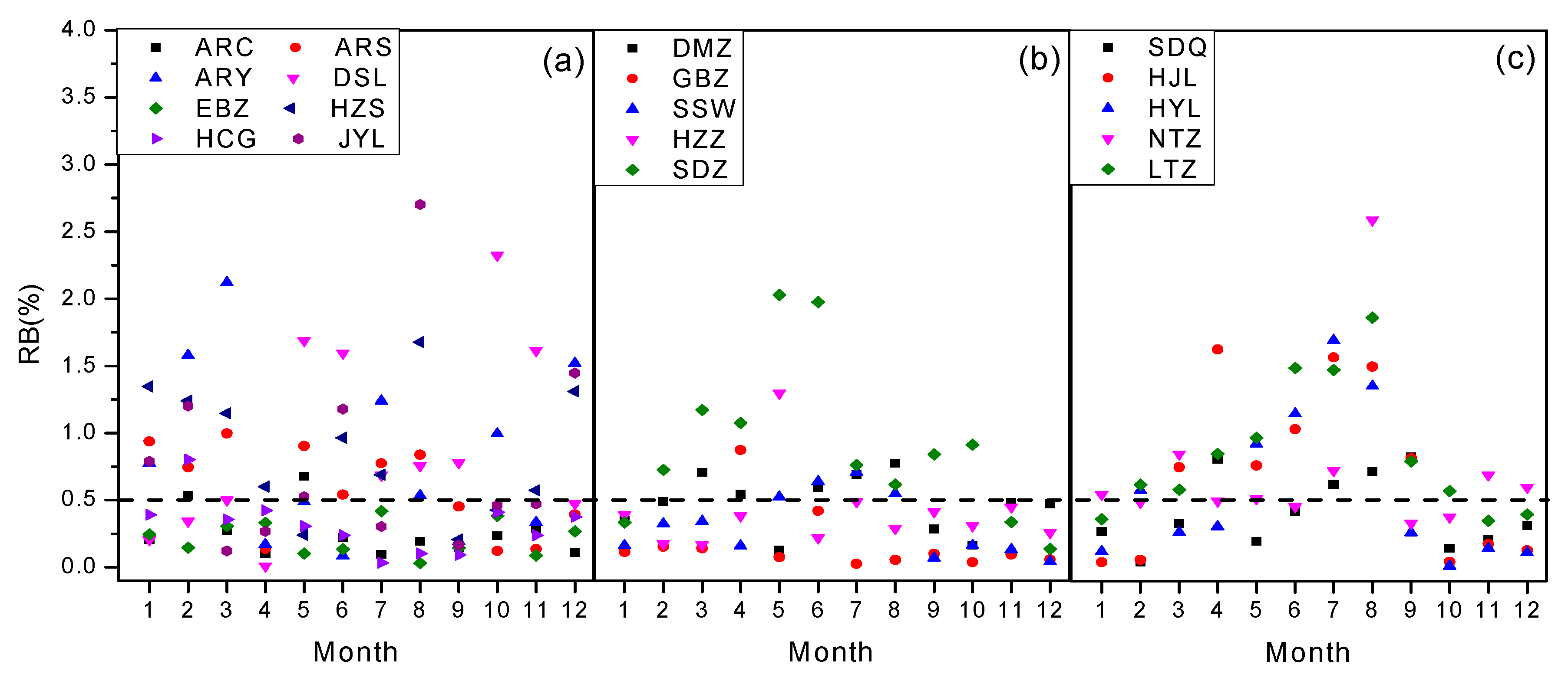
The RB values of the stations in the upstream area, midstream area, and downstream area and their monthly changes are shown in Figure 5a–c, respectively. The eight upstream stations did not show a consistent trend with vegetation growth. As shown in Table 1, the LCTs of these stations were mostly grass or meadows. The DLCT values of these stations were all greater than 80%, with the exception of HZS, and the area of the heat-shadow effect in the thermal-infrared image was wider than the actual area. The RB depended on the homogeneity of the vegetation density for the stations that were covered by only one vegetation type and its changes with the seasons. Many factors can influence the density’s homogeneity and its changes with vegetation growth, such as non-uniform rain or snow, random grazing in the grass, and uneven growth. Thus, complex factors are likely the main reasons for the inconsistency and volatility of the stations’ changing RB trends. The chance of an RB value below 0.5% was greatest for stations with a DLCT above 60%.
The monthly changes in the RB at the stations in the midstream and downstream areas of the HRB could be divided into two types (Figure 5b,c). The first type included GBZ, SSW and HZZ, with DLCT values of 100%. Their RB values showed similar trends to those of the upstream stations, with inconsistency and volatility. The RB values of these stations were mostly smaller than 0.5%. The RB values of the other midstream and downstream stations, which had smaller DLCT values, increased with the NDVI (shown in Figure 6), although the RB’s maximum peak point appeared within, before or after the month of the maximum NDVI peak. The RB values of these stations were all larger than 0.5% during the growing season. The land within a 1-km pixel area at these stations was covered by more than two LCTs, and the LST difference increased with vegetation growth and increasing solar radiation, especially at the maximum peak during summer. For instance, the midstream SDZ station was mainly covered by water and seeds. During winter, the station was predominantly covered by water, resulting in a small RB value below 0.5%. As the seeds began to grow, the seed area became larger, and the LST difference between seed and water increased as the solar radiance became stronger, creating a larger RB value. After reaching its maximum, the RB value decreased as vegetation growth and the solar radiance simultaneously decreased. The above analysis shows that the RB is relatively consistent with the DLCT and that an RB threshold is reasonable to effectively distinguish each level for a 1-km pixel.
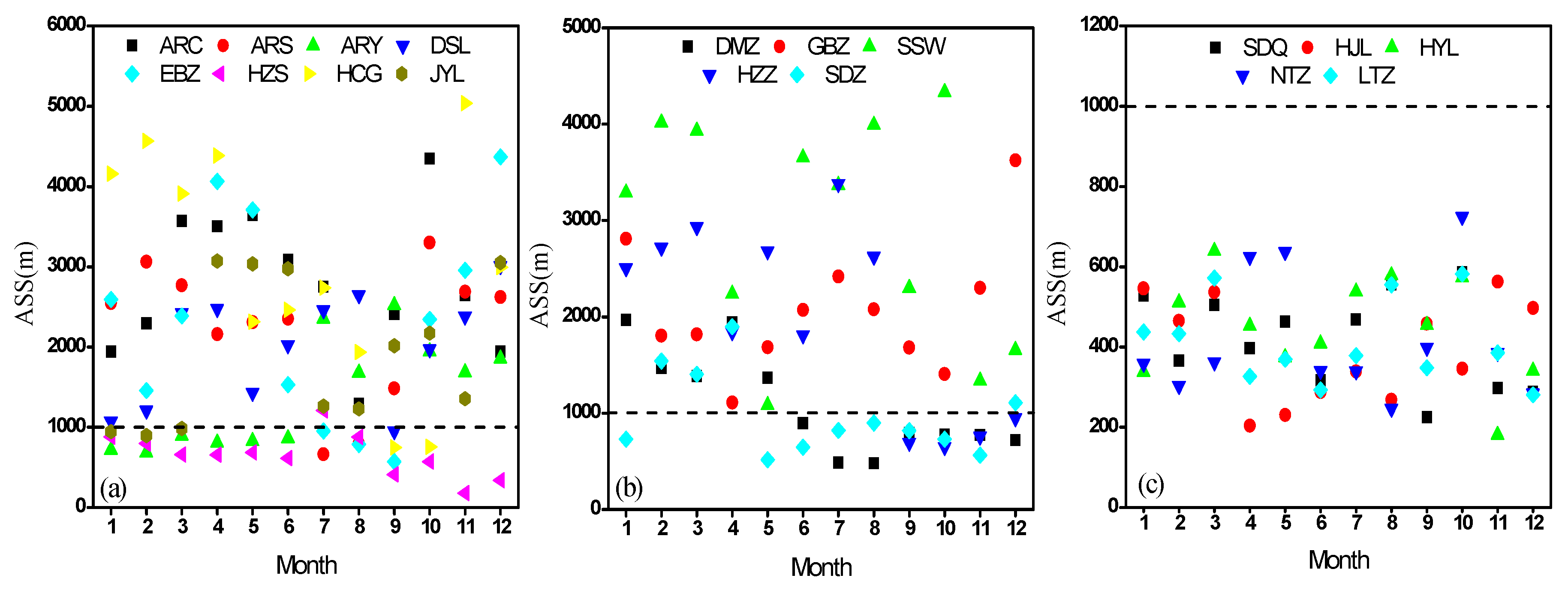
The monthly ASS values of all the stations in the HRB are shown in Figure 7, with the ASS plots of stations in the upstream area in Figure 7a, the ASS plots of stations in the midstream area in Figure 7b, and the ASS plots of stations in the downstream area in Figure 7c. The black dashed lines in Figure 7 are the threshold of the ASS. The ASS plots of each station in Figure 7 did not show consistent trends as the seasons changed. However, when the DLCT values of the stations were less than 60%, the corresponding ASS values were less than 1000 m. Even for stations with DLCT values of 100%, the ASS value could be smaller than 1000 m, such as JYL in January and February (see Figure 4a and Figure 6a). The ASS results for the stations were determined by the heterogeneity in the 1-km LST pixel. The heterogeneity of stations with a DLCT below 60% was mainly caused by the LST differences among different LCTs in the pixel. By contrast, the heterogeneity of stations with greater DLCT values, including values of 100%, was determined by the density heterogeneity of the dominant vegetation in the pixel, which is influenced by many factors, including uneven vegetation growth, human activity, such as random grazing, and localized weather, such as non-uniform rainfall. Moreover, the results were affected by the combination of these factors, leading to fluctuating ASS plot trends for stations with DLCT values of 100%.
The monthly representativeness levels of the multi-temporal LST observations of all the stations in the HRB are shown in Figure 8 based on the DLCT values and the monthly RB and ASS values, which were calculated using the high-resolution LST images from the Landsat 8 images. Eight stations were present in the upstream area, so the upstream stations were divided into two figures, namely, Figure 8a,b, to clearly show the monthly representativeness. The monthly representativeness levels of the midstream and downstream stations are shown in Figure 8c,d. All the downstream stations had DLCT values below 60%, so all the stations are listed as Level 5 in Figure 8d. The spatial representativeness varied by month for the different stations. Among the 216 months of observations (18 stations in 12 months from September 2013 to September 2014), only 73 months of observations were graded as Level 1, so the number of station observations that perfectly represented the pixel were limited.
4.3. Traditional Validation Results without Spatial Representative Assessment
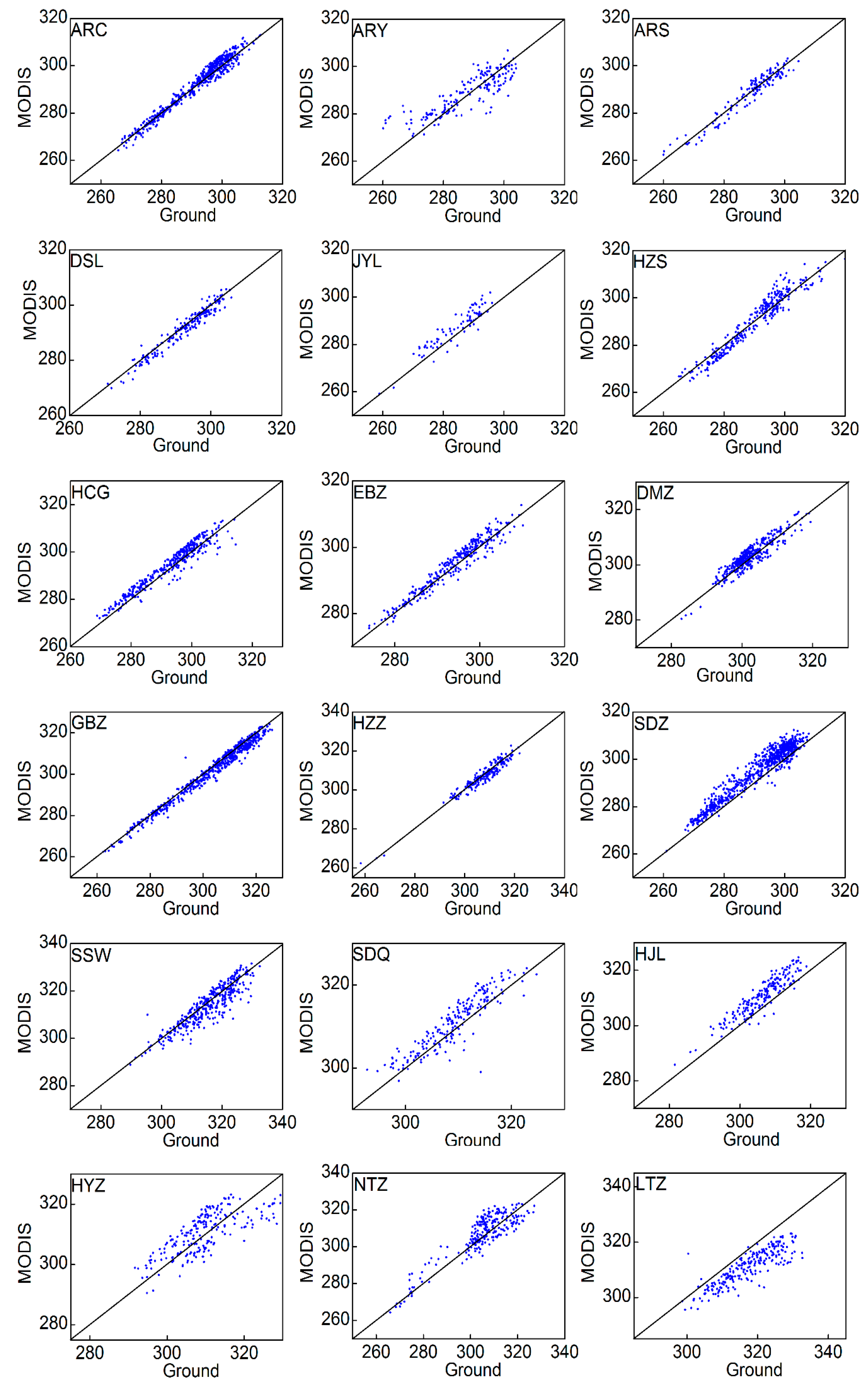
Traditional initial validation results, which neglect the evaluation of the spatial representativeness of the station observations, are presented first to demonstrate the effectiveness of our proposed scheme. The scatter plots in Figure 9 and Figure 10 show the daytime and nighttime comparison results between the MODIS LST and ground-based LST measurements. As shown in Figure 8, the scatters in half of the sub-plots were close to the 1:1 line (the black line in the scatter plot). By contrast, the scatters for ARY, JYL, SDZ, SSW, SDQ, HJL, HYZ, NTZ, and LTZ were more decentralized. In Figure 10, the scatters of these sites were closer to the 1:1 line than those in Figure 9. Table 3 presents a statistical comparison of the daytime and nighttime results between the ground-based measurements and MODIS LST products that were retrieved from the MODIS data onboard Terra and Aqua, respectively. The bias (ground-based LST measurements—MODIS LST) at eighteen sites during the daytime ranged between −4.72 K and 6.46 K for the MOD11A1 LST/LSE products and between −3.44 K and 6.24 K for the MYD11A1 LST/LSE products; the root mean square error (RMSE) during the daytime ranged from 1.74 K to 5.50 K for the Terra MODIS LSTs (MOD11A1 LST/LSE products) and from 1.75 K to 5.94 K for the Aqua MODIS LSTs (MYD11A1 LST/LSE products). By contrast, the bias and RMSE between the Terra MODIS LST and ground-based measurements at nighttime ranged from −0.51 K to 3.86 K and from 1.19 K to 2.64 K, respectively; for the Aqua MODIS LST, the bias ranged from −0.39 K to 3.48 K and the RMSE ranged from 1.94 K to 3.82 K.
The initial results revealed that the MODIS LSTs fit better with MODIS at nighttime than during the daytime, and the comparison results greatly differed between the daytime and nighttime for some stations, especially HZS, HYZ, NTZ, and LTZ, which are all Level-5 stations. The LST had stronger heterogeneity during the daytime than at nighttime. During the day, LSTs can vary by 10 K or more over a few meters depending on the nature of the surface and the local meteorological conditions, with the variability being lower at night [9]. When comparing the unrepresentative observations of these stations to the MODIS LSTs, the stronger heterogeneity resulted in greater differences in the bias and RMSEs of these stations between the daytime and nighttime because of the constant accuracy of the MODIS LST products within the same pixel. If these results were considered the final results for the accuracy of the MODIS LST, an obvious error would be introduced into the validation because of the unrepresentativeness of the station observations when compared to the corresponding scale of the remote-sensing observations. The stronger heterogeneity during the daytime affected the Aqua MODIS LST and Terra MODIS LST validation process in a similar manner, so no significant differences in accuracy existed between the LST products from Terra MODIS and the LST products from Aqua MODIS when compared to the ground-measured LSTs at these sites, as shown in Table 3.
4.4. MODIS LST Product Validation Considering the Influence of Spatial Representativeness Evaluation
All the station observation validation results and representative station observation validation results were calculated and compared to discuss the effect of representativeness on the validation of satellite-retrieved LSTs. In total, 7527 station observations from eighteen stations were evaluated based on the Landsat 8 LST reference maps according to the satellite-overpass times and quality control flags of the MODIS LSTs. The RMSE and bias of the MOD/MYD11A1 LST products based on all the observations and the different levels of observations are listed in Table 4. For all the observations, the bias of the MODIS LST ranged from −0.27 K to 2.39 K, and the RMSE ranged from 3.32 K to 4.93 K. The RMSEs were the smallest for Level 1, which contained 2472 station observations. During both the daytime and nighttime, the bias between the station observations and MODIS LSTs was better than 1 K and the RMSE was less than 2 K. No significant differences existed between the daytime and nighttime comparison results for the Level 1 observations. These results using Level 1 observations are inconsistent with those from the traditional validation scheme in Section 4.3 and are more reasonable based on the retrieval accuracy of the MODIS LSTs during the daytime and nighttime for the same pixel. The comparison results between the MODIS LSTs and LST observations for Levels 2 and 3 had a similar bias and RMSE, which were not larger than those for all the observations. The results for the Level-4 observations had a larger bias and RMSE than those for Levels 3 and 2. The largest RMSE values were obtained when using Level 5 observations. The RMSE value increased from Level 1 to Level 5. Large differences existed in the bias and RMSE between the daytime and nighttime at all levels, except for Level 1, because of the greater spatial heterogeneity during the daytime. Table 4 indicates that the highly representative validated observations usually had good results. Thus, highly representative observations can more accurately describe satellite-retrieved LST values and limit spatial mismatch errors from point-station observations. Therefore, validating all the stations without grading their representativeness usually underestimated the accuracy of the satellite-retrieved LSTs; these underestimated accuracy values were larger for the daytime validation than the nighttime validation.
4.5. Other Potential Factors during the LST Validation Process
Other factors may potentially influence the accuracy of the validation results. In this study, we only focused on the sensor view zenith angle (VZA) and broadband sensitivity issues, which are the main factors that affect T-based validation for MODIS LSTs in addition to the representativeness of the station observations. The effects of these two factors are discussed in detail below.
4.5.1. Dependence of the LST Error on the Sensor VZA
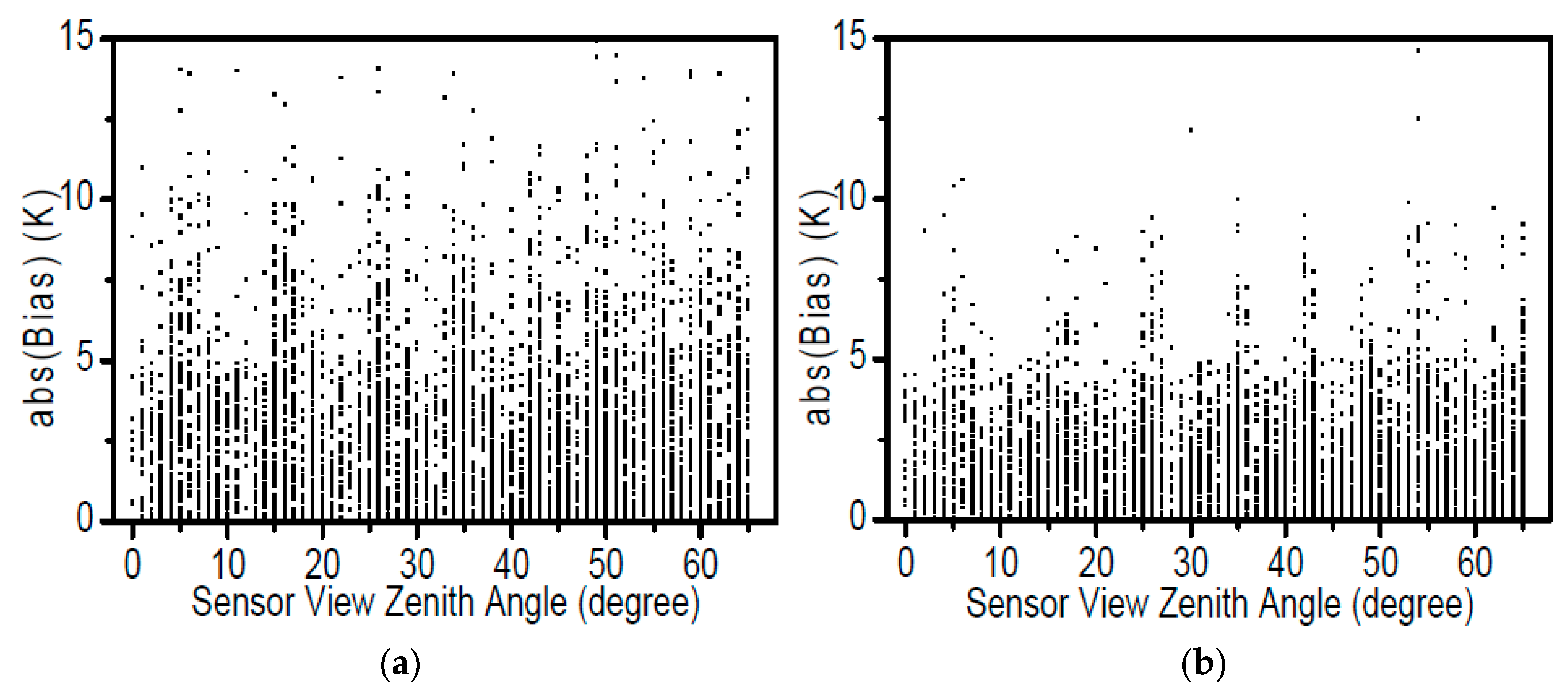
The relationship between the error (the absolute difference between MODIS and ground-based LSTs) and the sensor VZA was first investigated at all HiWATER sites to analyze the potential factors that create large errors at certain sites. The VZAs differed between ground-based instruments and the MODIS sensor: the ground-measured LSTs were obtained at a VZA of 0°, whereas the MODIS observations were acquired over a large range of VZAs (0–65°). Sufficient ground-based measurements were available to statistically analyze multiple VZAs using data from the eighteen sites. Scatterplots of the errors and sensor VZAs are presented in Figure 11. The average errors did not significantly depend on the VZAs during the daytime (see Figure 11a). By contrast, the probability of a larger error increased with the VZA for the nighttime scatterplot (Figure 11b). The average absolute bias for observations that were acquired with a smaller VZA (≤30°) was 0.2 K lower than that for those at greater VZAs (>30°). Greater errors for LSTs observed under larger sensor VZAs were also observed in a prior validation study [8,13], and the remote sensor may see different percentages of shadows at different VZAs during the daytime, when larger heterogeneities occur [58]. The larger LST heterogeneity at certain sites was the most likely cause of the daytime scatterplot (Figure 11a), rather than the obvious dependence of the error of the LST on the sensor VZA.
4.5.2. Broadband Sensitivity Issue
The accuracy of LSTs from ground-based longwave-radiation measurements is another important factor that influences the evaluation of MODIS LSTs. The accuracy of longwave-radiation measurements and the accuracy of the broadband emissivity, which is used to calculate LSTs from ground-based longwave-radiation measurements, are the two major factors for ground-based LST estimation. The accuracy of longwave-radiation measurements depends on the sensor calibration. Calibration is typically performed before and after field deployment and during monthly field-routing exams [59], so the estimation accuracy of the broadband emissivity is a key parameter that influences the estimation accuracy of ground-based LST observations. Our previous study indicated that the maximum mean absolute error (MAE) of the LST was less than 0.3 K when the estimation emissivity MAE was ≤0.01, which was estimated by adding a series bias of ±0.001, ±0.002, ±0.003, ±0.004, ±0.005, and ±0.01 based on the values at the stations in the northern arid region of China, including ARC, HZZ, and DMZ (also called YK) [60]. In this study, the satellite-estimated broadband-emissivity method was used based on the MODIS narrowband emissivities. A suitable set of coefficients for all the data was used to calculate the broadband emissivity, as outlined in Equation (7), according to the diversity of the land cover at the sites. In a study by Wang et al., the broadband emissivity that was estimated by this method was compared to three years of ground-based emissivity measurements at Gaize (32.30°N and 84.06°E, with an elevation of 4420 m) in the western Tibetan Plateau. The results showed that the broadband-emissivity calculation from the MODIS narrowband emissivities reasonably matched the ground measurements, with a standard deviation of 0.0085 and a bias of 0.0015 [45]. Therefore, the average estimation error of the broadband emissivity based on this method was less than 0.037 K, which is the maximum average absolute error value of all the stations in northern arid China for an emissivity bias of 0.02.
5. Conclusions
In traditional validation schemes, as discussed in Section 4.3, station observations are usually considered as the true LST values of the corresponding pixels. Therefore, a source of uncertainty for the validation results is introduced when the representativeness of station observations is not evaluated. The spatial representativeness assessment of station observations is a key step to reliably validate satellite-retrieved LST products, which has barely been discussed by previous researchers. In this study, a new validation scheme was proposed that adds a key step to evaluate the spatial representativeness of station LST observations. Three indicators, namely, the DLCT, RB, and ASS, were constructed in this new scheme to assess and grade the representativeness of station observations. The representativeness of the station observations was divided into five levels for a 1-km spatial resolution pixel according to the values of these three indicators. Then, the proposed method was used to evaluate the spatial representativeness of HiWATER LST observations for 1-km-pixel daily MODIS LST products. The analysis showed that the new validation scheme can effectively limit the error that is introduced by spatial mismatches between the station observations and remote-sensing products. This spatial representative assessment synthesized the three indicators, providing quantitative and accurate descriptions and reliably evaluating the observations’ representativeness, although reasonable thresholds for the three indicators should consider the LST products’ spatial resolution, the theoretical accuracy of the retrieval algorithm, and instrument error. Therefore, several conclusions can be drawn.
First, the traditional validation results when using all the station observations showed obvious errors and RMSE values between the daytime and nighttime validations, especially when using observations from the downstream stations. The retrieval method for the MODIS LST products could obtain LST products with similar accuracy during the daytime and nighttime. Therefore, the error was likely introduced by unrepresentative station observations. According to the HRB traditional validation sample, this effect caused a maximum bias of 8.03 K and a maximum RMSE of 3.25 K according to the difference between the daytime and nighttime validation results from the same stations.
Second, the monthly representativeness analysis illustrated that the spatial contexture heterogeneity and point-to-pixel consistency of the LST changed with variations in plant growth and other factors, such as human activity, the solar-radiation intensity, and the local climate, which created irregular changes in the monthly spatial representativeness of the stations. The monthly changes in all the factors that influenced the representativeness were not always similar between consecutive years, so the spatial representativeness in the same month of different years may have greatly changed for a given station. Therefore, the spatial representativeness for consecutive years could be reassessed through a rigorous LST product-validation process.
Third, the RMSE of the MOD/MYD11A1 products increased from 1.58 K to 6.27 K from Level 1 to Level 5, and the RMSE values from Level 1 to Level 3 were smaller than those across all the observations. For all levels except Level 1, the RMSE values were larger during the daytime than those at nighttime because of the stronger LST heterogeneity during the daytime. The obvious differences in the bias and RMSE values among the levels indicated that the representativeness method could sufficiently differentiate the spatial representativeness level within 1-km pixels. Moreover, the Level-1 LST observations were acceptable validation data for the MODIS 1-km LST products. While the RMSE difference between all observations (using in the traditional validations) and Level 1 observations validations are 3.0 K in daytime and 1.7 K in nighttime, which indicates the error introduced by the traditional validation without the representativeness assessment. Therefore, the error of the MOD/MYD11A1 products was better than 1 K and the RMSE was less than 2 K. Moreover, no obvious differences existed in the accuracy of the MODIS LST products among the four daily times that Terra and Aqua passed.
Finally, the bias increased from −0.19 K at Level 1 to 3.6 K at Level 5, and the RMSE increased from 1.58 to 6.27. Thus, a bias difference of 3.79 K and a RMSE difference of 4.69 K existed between Level 1, which was the most representative level, and Level 5, which was the least representative level. The dependence of the absolute biases on the sensor VZA during the daytime was strongly influenced by the land-surface heterogeneity at heterogeneous sites. During the nighttime, the LSTs of these sites were more homogeneous and any surface-heterogeneity effects were smaller, so the average absolute bias for observations that were acquired under lower VZA (≤30°) was 0.2 K lower than those that were acquired at greater VZAs (>30°). The estimated broadband emissivities from the narrowband MODIS LST/LSE products retrieved by the day/night algorithm varied with the land-surface conditions, such as vegetation growth and land cover, with a bias of 0.0015. Therefore, the estimation error of the broadband emissivities was less than 0.004 K. Compared to the effects of the representativeness, the errors from these last two factors were very small. Thus, the evaluation of spatial representativeness is a key step to reliably validate LST products with special spatial resolution, which is the greatest advantage of our proposed validation scheme.
A more reasonable and accurate scheme to validate remotely sensed LST products was proposed in this study. However, areas with more heterogeneous LSTs are not suitable for validation with single-point ground-based measurements and require conditional upscaling by multi-point ground-based measurements. Therefore, this scheme can be further improved for different conditions, and can be actually used to study potential new sites for LST validation. Furthermore, the thresholds of the three indicators were suitable for grading the levels of station observations in a 1-km pixel. This scheme can also be used to evaluate other LST products by renewing the thresholds and evaluating the spatial representativeness in other pixel grids.
Acknowledgments
This work was supported by the Natural Science Foundation of China (Grant No. 41601448), the National Key Technology R&D Program of China (Grant No. 2016YFC0500106), the Fundamental Research Funds for the Central Universities of China (Grant No. XDJK2016C094) and the Doctoral Fund of Southwest University (Grant No. SWU115063). This study was also supported by the China Scholarship Council. The authors would like to thank all the institutes and universities in the North Arid and Semi-Arid Area Cooperative Experimental Observation Integrated Research Program for providing the meteorological data.
Author Contributions
Mingguo Ma outlined the research topic and assisted with manuscript writing. Zhaoliang Li gave much helpful advice on the revising work. Junlei Tan and Adan Wu were involved in the data collection and preprocessing step. Wenping Yu processed the data, analyzed the results and wrote the manuscript.
Conflicts of Interest
The authors declare no conflict of interest.
References
- Liang, S.L. Quantitative Remote Sensing of Land Surface; John Wiley & Sons: Hoboken, NJ, USA, 2004. [Google Scholar]
- Smith, P.M.; Kalluri, S.N.V.; Prince, S.; Defries, R. The NOAA/NASA pathfinder AVHRR 8-km land data set. Photogramm. Eng. Remote Sens. 1997, 63, 12–27. [Google Scholar]
- El Saleous, N.; Vermote, E.; Justice, C.; Townshend, J.; Tucker, C.; Goward, S. Improvements in the global biospheric record from the Advanced Very High Resolution Radiometer (AVHRR). Int. J. Remote Sens. 2000, 21, 1251–1277. [Google Scholar] [CrossRef]
- Sun, D.; Pinker, R.T. Estimation of land surface temperature from a Geostationary Operational Environmental Satellite (GOES-8). J. Geophys. Res. Atmos. 2003, 108. [Google Scholar] [CrossRef]
- Sobrino, J.A.; Jiménez-Muñoz, J.C.; Sòria, G.; Romaguera, M.; Guanter, L.; Moreno, J.; Plaza, A.; Martínez, P. Land surface emissivity retrieval from different VNIR and TIR sensors. IEEE Trans. Geosci. Remote Sens. 2008, 46, 316–327. [Google Scholar] [CrossRef]
- Trigo, I.F.; Peres, L.F.; DaCamara, C.C.; Freitas, S.C. Thermal land surface emissivity retrieved from SEVIRI/Meteosat. IEEE Trans. Geosci. Remote Sens. 2008, 46, 307–315. [Google Scholar] [CrossRef]
- Li, Z.-L.; Tang, B.-H.; Wu, H.; Ren, H.; Yan, G.; Wan, Z.; Trigo, I.F.; Sobrino, J.A. Satellite-derived land surface temperature: Current status and perspectives. Remote Sens. Environ. 2013, 131, 14–37. [Google Scholar] [CrossRef]
- Coll, C.; Caselles, V.; Galve, J.M.; Valor, E.; Niclos, R.; Sanchez, J.M.; Rivas, R. Ground measurements for the validation of land surface temperatures derived from AATSR and MODIS data. Remote Sens. Environ. 2005, 97, 288–300. [Google Scholar] [CrossRef]
- Coll, C.; Wan, Z.; Galve, J.M. Temperature-based and radiance-based validations of the v5 MODIS land surface temperature product. J. Geophys. Res. Atmos. 2009, 114. [Google Scholar] [CrossRef]
- Wan, Z. New refinements and validation of the collection-6 MODIS land-surface temperature/emissivity product. Remote Sens. Environ. 2014, 140, 36–45. [Google Scholar] [CrossRef]
- Wan, Z.; Zhang, Y.; Zhang, Q.; Li, Z.L. Quality assessment and validation of the MODIS global land surface temperature. Int. J. Remote Sens. 2004, 25, 261–274. [Google Scholar] [CrossRef]
- Wang, K.; Liang, S. Evaluation of ASTER and MODIS land surface temperature and emissivity products using long-term surface longwave radiation observations at SURFRAD sites. Remote Sens. Environ. 2009, 113, 1556–1565. [Google Scholar] [CrossRef]
- Wang, W.; Liang, S.; Meyers, T. Validating MODIS land surface temperature products using long-term nighttime ground measurements. Remote Sens. Environ. 2008, 112, 623–635. [Google Scholar] [CrossRef]
- Wan, Z. New refinements and validation of the MODIS land-surface temperature/emissivity products. Remote Sens. Environ. 2008, 112, 59–74. [Google Scholar] [CrossRef]
- Wang, S.; Li, X.; Ge, Y.; Jin, R.; Ma, M.; Liu, Q.; Wen, J.; Liu, S. Validation of regional-scale remote sensing products in China: From site to network. Remote Sens. 2016, 8, 980. [Google Scholar] [CrossRef]
- Gupta, R.K.; Prasad, T.S.; Krishna Rao, P.V.; Bala Manikavelu, P.M. Problems in upscaling of high resolution remote sensing data to coarse spatial resolution over land surface. Adv. Space Res. 2000, 26, 1111–1121. [Google Scholar] [CrossRef]
- Liu, Y.; Hiyama, T.; Yamaguchi, Y. Scaling of land surface temperature using satellite data: A case examination on ASTER and MODIS products over a heterogeneous terrain area. Remote Sens. Environ. 2006, 105, 115–128. [Google Scholar] [CrossRef]
- Liu, Y.B.; Yamaguchi, Y.; Ke, C.Q. Reducing the discrepancy between aster and MODIS land surface temperature products. Sensors 2007, 7, 3043–3057. [Google Scholar] [CrossRef] [PubMed]
- Hook, S.J.; Vaughan, R.G.; Tonooka, H.; Schladow, S.G. Absolute radiometric in-flight validation of mid infrared and thermal infrared data from ASTER and MODIS on the terra spacecraft using the Lake Tahoe, CA/NV, USA, automated validation site. IEEE Trans. Geosci. Remote Sens. 2007, 45, 1798–1807. [Google Scholar] [CrossRef]
- Yu, W.; Ma, M. Scale mismatch between in situ and remote sensing observations of land surface temperature: Implications for the validation of remote sensing LST products. IEEE Geosci. Remote Sens. Lett. 2015, 12, 497–501. [Google Scholar]
- Xu, B.; Li, J.; Liu, Q.; Huete, A.R.; Yu, Q.; Zeng, Y.; Yin, G.; Zhao, J.; Yang, L. Evaluating spatial representativeness of station observations for remotely sensed leaf area index products. IEEE J. Sel. Top. Appl. Earth Obs. Remote Sens. 2016, 9, 3267–3282. [Google Scholar] [CrossRef]
- Hakuba, M.Z.; Folini, D.; Sanchez-Lorenzo, A.; Wild, M. Spatial representativeness of ground-based solar radiation measurements. J. Geophys. Res. Atmos. 2013, 118, 8585–8597. [Google Scholar] [CrossRef]
- Román, M.O.; Schaaf, C.B.; Woodcock, C.E.; Strahler, A.H.; Yang, X.; Braswell, R.H.; Curtis, P.S.; Davis, K.J.; Dragoni, D.; Goulden, M.L. The MODIS (Collection V005) BRDF/albedo product: Assessment of spatial representativeness over forested landscapes. Remote Sens. Environ. 2009, 113, 2476–2498. [Google Scholar] [CrossRef]
- Janis, M.J.; Robeson, S.M. Determining the spatial representativeness of air-temperature records using variogram-nugget time series. Phys. Geogr. 2004, 25, 513–530. [Google Scholar] [CrossRef]
- Henne, S.; Brunner, D.; Folini, D.; Solberg, S.; Klausen, J.; Buchmann, B. Assessment of parameters describing representativeness of air quality in-situ measurement sites. Atmos. Chem. Phys. 2010, 10, 3561–3581. [Google Scholar] [CrossRef] [Green Version]
- Jia, Z.; Liu, S.; Xu, Z.; Chen, Y.; Zhu, M. Validation of remotely sensed evapotranspiration over the Hai River Basin, China. J. Geophys. Res. Atmos. 2012, 117. [Google Scholar] [CrossRef]
- Janssen, S.; Dumont, G.; Fierens, F.; Deutsch, F.; Maiheu, B.; Celis, D.; Trimpeneers, E.; Mensink, C. Land use to characterize spatial representativeness of air quality monitoring stations and its relevance for model validation. Atmos. Environ. 2012, 59, 492–500. [Google Scholar] [CrossRef]
- Chan, C.-C.; Hwang, J.-S. Site representativeness of urban air monitoring stations. J. Air Waste Manag. Assoc. 1996, 46, 755–760. [Google Scholar] [CrossRef] [PubMed]
- Wang, Z.; Schaaf, C.B.; Chopping, M.J.; Strahler, A.H.; Wang, J.; Roman, M.O.; Rocha, A.V.; Woodcock, C.E.; Shuai, Y. Evaluation of Moderate-resolution Imaging Spectroradiometer (MODIS) snow albedo product (MCD43A) over tundra. Remote Sens. Environ. 2012, 117, 264–280. [Google Scholar] [CrossRef]
- Chen, B.; Coops, N.C.; Fu, D.; Margolis, H.A.; Amiro, B.D.; Black, T.A.; Arain, M.A.; Barr, A.G.; Bourque, C.P.-A.; Flanagan, L.B. Characterizing spatial representativeness of flux tower eddy-covariance measurements across the Canadian Carbon Program Network using remote sensing and footprint analysis. Remote Sens. Environ. 2012, 124, 742–755. [Google Scholar] [CrossRef]
- Cescatti, A.; Marcolla, B.; Vannan, S.K.S.; Pan, J.Y.; Román, M.O.; Yang, X.; Ciais, P.; Cook, R.B.; Law, B.E.; Matteucci, G. Intercomparison of MODIS albedo retrievals and in situ measurements across the global FLUXNET network. Remote Sens. Environ. 2012, 121, 323–334. [Google Scholar] [CrossRef]
- Wang, Z.; Schaaf, C.B.; Strahler, A.H.; Chopping, M.J.; Román, M.O.; Shuai, Y.; Woodcock, C.E.; Hollinger, D.Y.; Fitzjarrald, D.R. Evaluation of MODIS albedo product (MCD43A) over grassland, agriculture and forest surface types during dormant and snow-covered periods. Remote Sens. Environ. 2014, 140, 60–77. [Google Scholar] [CrossRef]
- Li, X.; Cheng, G.; Liu, S.; Xiao, Q.; Ma, M.; Jin, R.; Che, T.; Liu, Q.; Wang, W.; Qi, Y.; et al. Heihe watershed allied telemetry experimental research (HiWATER): Scientific objectives and experimental design. Bull. Am. Meteorol. Soc. 2013, 94, 1145–1160. [Google Scholar] [CrossRef]
- Journel, A.G.; Huijbregts, C.J. Mining Geostatistics; Academic Press: London, UK, 1981. [Google Scholar]
- Cressie, N. The origins of kriging. Math. Geol. 1990, 22, 239–252. [Google Scholar] [CrossRef]
- Rossi, R.E.; Mulla, D.J.; Journel, A.G.; Franz, E.H. Geostatistical tools for modeling and interpreting ecological spatial dependence. Ecol. Monogr. 1992, 62, 277–314. [Google Scholar] [CrossRef]
- Robertson, G.P. Geostatistics in ecology: Interpolating with known variance. Ecology 1987, 68, 744–748. [Google Scholar] [CrossRef]
- Curran, P.J.; Atkinson, P.M. Geostatistics and remote sensing. Prog. Phys. Geogr. 1998, 22, 61–78. [Google Scholar] [CrossRef]
- Atkinson, P.M.; Tate, N.J. Spatial scale problems and geostatistical solutions: A review. Prof. Geogr. 2000, 52, 607–623. [Google Scholar] [CrossRef]
- Burcsu, T.K.; Robeson, S.M.; Meretsky, V.J. Identifying the distance of vegetative edge effects using Landsat TM data and geostatistical methods. Geocarto Int. 2001, 16, 61–70. [Google Scholar] [CrossRef]
- Li, H.; Reynolds, J. On definition and quantification of heterogeneity. Oikos 1995, 73, 280–284. [Google Scholar] [CrossRef]
- Hu, Y.D.; Gao, J.M.; Wang, J.M.; Ji, G.L.; Shen, Z.B.; Cheng, L.S.; Chen, J.Y.; Li, S.Q. Some achievements in scientific research during HEIFE. Plateau Meteorol. 1994, 13, 225–236. [Google Scholar]
- Li, X.; Li, X.; Li, Z.; Ma, M.; Wang, J.; Xiao, Q.; Liu, Q.; Che, T.; Chen, E.; Yan, G.; et al. Watershed allied telemetry experimental research. J. Geophys. Res. 2009, 114. [Google Scholar] [CrossRef]
- Heihe Watershed Allied Telemetry Experimental Research (HiWATER) Home. Available online: http://card.westgis.ac.cn/hiwater (accessed on 17 March 2017).
- Wang, K.; Wan, Z.; Wang, P.; Sparrow, M.; Liu, J.; Zhou, X.; Haginoya, S. Estimation of surface long wave radiation and broadband emissivity using Moderate Resolution Imaging Spectroradiometer (MODIS) land surface temperature/emissivity products. J. Geophys. Res. Atmos. 2005, 110, D11109. [Google Scholar] [CrossRef]
- Salomonson, V.V.; Barnes, W.; Maymon, P.W.; Montgomery, H.E.; Ostrow, H. Modis: Advanced facility instrument for studies of the earth as a system. IEEE Trans. Geosci. Remote Sens. 1989, 27, 145–153. [Google Scholar] [CrossRef]
- Wan, Z.M.; Dozier, J. A generalized split-window algorithm for retrieving land-surface temperature from space. IEEE Trans. Geosci. Remote Sens. 1996, 34, 892–905. [Google Scholar]
- Wan, Z.M.; Li, Z.L. A physics-based algorithm for retrieving land-surface emissivity and temperature from EOS/MODIS data. IEEE Trans. Geosci. Remote Sens. 1997, 35, 980–996. [Google Scholar]
- Seemann, S.W.; Li, J.; Gumley, L.E.; Strabala, K.I.; Menzel, W.P. Operational retrieval of atmospheric temperature, moisture, and ozone from MODIS infrared radiances. J. Appl. Meteorol. 2003, 42, 1072–1091. [Google Scholar] [CrossRef]
- HiWATER: Land Cover Map of Heihe River Basin. Available online: http://card.westgis.ac.cn/hiwater/rsproduct (accessed on 21 March 2017).
- Zhong, B.; Ma, P.; Nie, A.; Yang, A.; Yao, Y.; Lü, W.; Zhang, H.; Liu, Q. Land cover mapping using time series HJ-1/CCD data. Sci. China Earth Sci. 2014, 57, 1790–1799. [Google Scholar] [CrossRef]
- Zhong, B.; Yang, A.; Nie, A.; Yao, Y.; Zhang, H.; Wu, S.; Liu, Q. Finer resolution land-cover mapping using multiple classifiers and multisource remotely sensed data in the Heihe River Basin. IEEE J. Sel. Top. Appl. Earth Obs. Remote Sens. 2015, 8, 4973–4992. [Google Scholar] [CrossRef]
- Zhong, B.; Zhang, Y.; Du, T.; Yang, A.; Lv, W.; Liu, Q. Cross-calibration of HJ-1/CCD over a desert site using Landsat ETM + Imagery and ASTER GDEM product. IEEE Trans. Geosci. Remote Sens. 2014, 52, 7247–7263. [Google Scholar] [CrossRef]
- Roy, D.P.; Wulder, M.; Loveland, T.; Woodcock, C.; Allen, R.; Anderson, M.; Helder, D.; Irons, J.; Johnson, D.; Kennedy, R. Landsat-8: Science and product vision for terrestrial global change research. Remote Sens. Environ. 2014, 145, 154–172. [Google Scholar] [CrossRef]
- Du, C.; Ren, H.; Qin, Q.; Meng, J.; Zhao, S. A practical split-window algorithm for estimating land surface temperature from Landsat 8 data. Remote Sens. 2015, 7, 647–665. [Google Scholar] [CrossRef]
- USGS Home. Available online: https://glovis.usgs.gov/ (accessed on 4 February 2017).
- MODIS Land Cover Product Algorithm Theoretical Basis Document (ATBD) Version 5.0. Available online: http://modis.gsfc.nasa.gov/data/atbd/land_atbd.php (accessed on 2 May 2016).
- Ermida, S.L.; Trigo, I.F.; DaCamara, C.C.; Göttsche, F.M.; Olesen, F.S.; Hulley, G. Validation of remotely sensed surface temperature over an oak woodland landscape—The problem of viewing and illumination geometries. Remote Sens. Environ. 2014, 148, 16–27. [Google Scholar] [CrossRef]
- Xu, Z.W.; Liu, S.M.; Li, X.; Shi, S.J.; Wang, J.M.; Zhu, Z.L.; Xu, T.R.; Wang, W.Z.; Ma, M.G. Intercomparison of surface energy flux measurement systems used during the HiWATER-MUSOEXE. J. Geophys. Res. 2013, 118, 13140–13157. [Google Scholar] [CrossRef]
- Yu, W.; Ma, M.; Wang, X.; Geng, L.; Tan, J.; Shi, J. Evaluation of MODIS LST products using longwave radiation ground measurements in the northern arid region of China. Remote Sens. 2014, 6, 11494–11517. [Google Scholar] [CrossRef]
Figure 1.
New scheme for land surface temperature (LST) validation based on the assessment of local spatial representativeness (site level). In the scheme, LCT is the abbreviation of land-cover type, and NDVI is the abbreviation of normalized difference vegetation index.
Figure 1.
New scheme for land surface temperature (LST) validation based on the assessment of local spatial representativeness (site level). In the scheme, LCT is the abbreviation of land-cover type, and NDVI is the abbreviation of normalized difference vegetation index.

Figure 2.
Study area and locations of the validation stations.

Figure 3.
Photos of the 18 Heihe Watershed Allied Telemetry Experimental Research (HiWATER) stations. The two pyrgeometers that were used to record the longwave radiation were deployed at an average height of 6 m, with one facing upwards and the other facing downwards.
Figure 3.
Photos of the 18 Heihe Watershed Allied Telemetry Experimental Research (HiWATER) stations. The two pyrgeometers that were used to record the longwave radiation were deployed at an average height of 6 m, with one facing upwards and the other facing downwards.


Figure 4.
The dominant land cover type (DLCT) for the HiWATER stations.
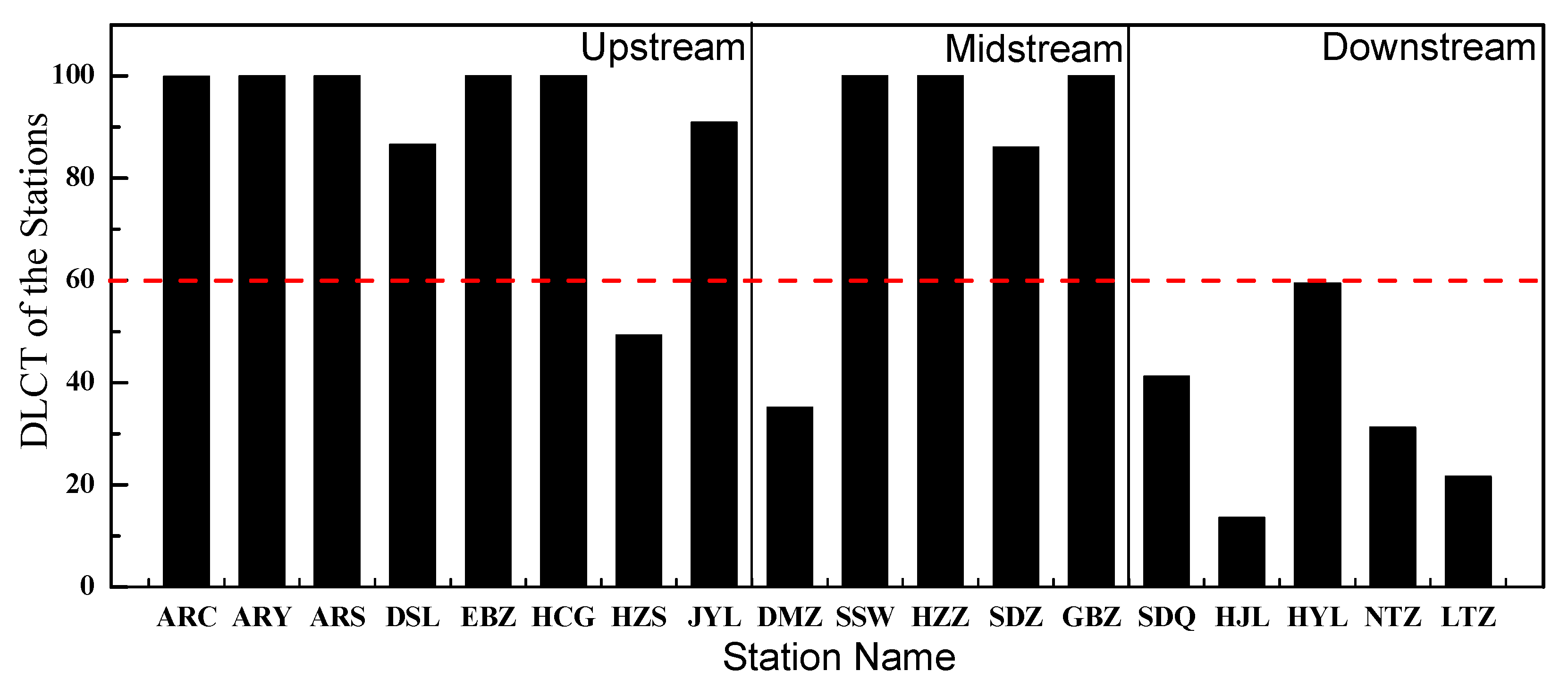
Figure 5.
Monthly relative bias (RB) of the observations from the 18 stations within 1-km MODIS LST pixels. (a), (b) and (c) respectively show the monthly RB of the stations in the upstream, midstream and downstream of the Heihe River Basin (HRB).
Figure 5.
Monthly relative bias (RB) of the observations from the 18 stations within 1-km MODIS LST pixels. (a), (b) and (c) respectively show the monthly RB of the stations in the upstream, midstream and downstream of the Heihe River Basin (HRB).

Figure 6.
Monthly normalized difference vegetation index (NDVI) at the eighteen sites from 2013 to 2014.
Figure 6.
Monthly normalized difference vegetation index (NDVI) at the eighteen sites from 2013 to 2014.

Figure 7.
Monthly average structure scale (ASS) of the stations. (a), (b) and (c) respectively show the monthly ASS of the stations in the upstream, midstream and downstream of the HRB.
Figure 7.
Monthly average structure scale (ASS) of the stations. (a), (b) and (c) respectively show the monthly ASS of the stations in the upstream, midstream and downstream of the HRB.

Figure 8.
Grading results of the stations. (a,b) show the monthly representativeness level of the upstream stations; (c,d) show the monthly representativeness level of midstream and downstream stations
Figure 8.
Grading results of the stations. (a,b) show the monthly representativeness level of the upstream stations; (c,d) show the monthly representativeness level of midstream and downstream stations
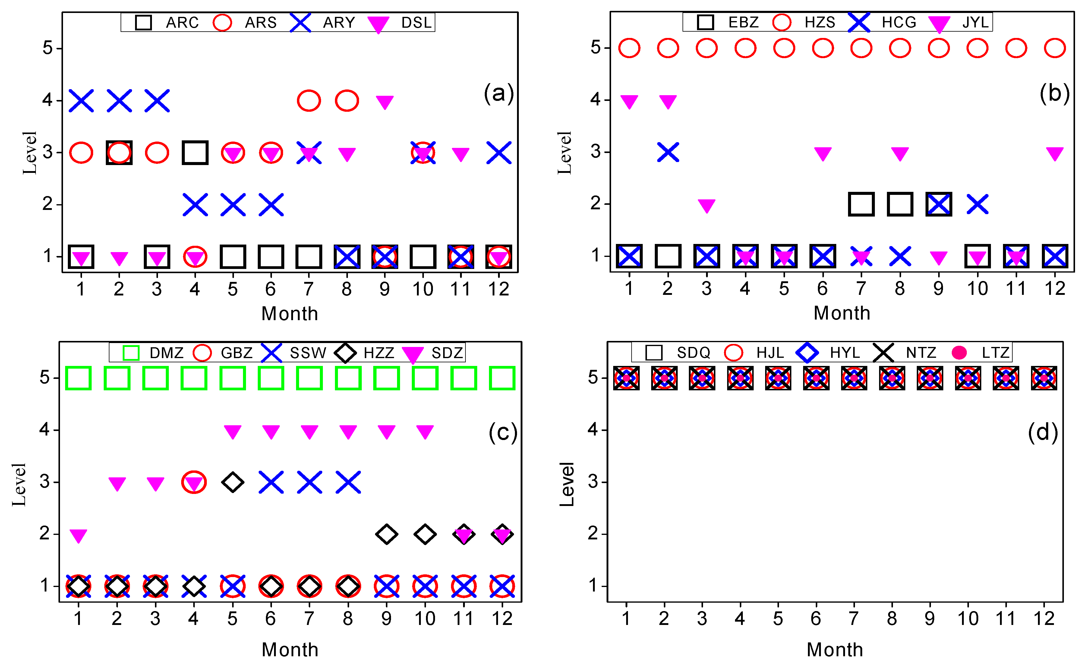
Figure 9.
Scatterplots of the daytime comparison results of the LSTs from MODIS and the LST measurements at the eighteen HiWATER sites.
Figure 9.
Scatterplots of the daytime comparison results of the LSTs from MODIS and the LST measurements at the eighteen HiWATER sites.

Figure 10.
Scatterplots of the nighttime comparison results of the LSTs from MODIS and the LST measurements at the eighteen HiWATER sites.
Figure 10.
Scatterplots of the nighttime comparison results of the LSTs from MODIS and the LST measurements at the eighteen HiWATER sites.
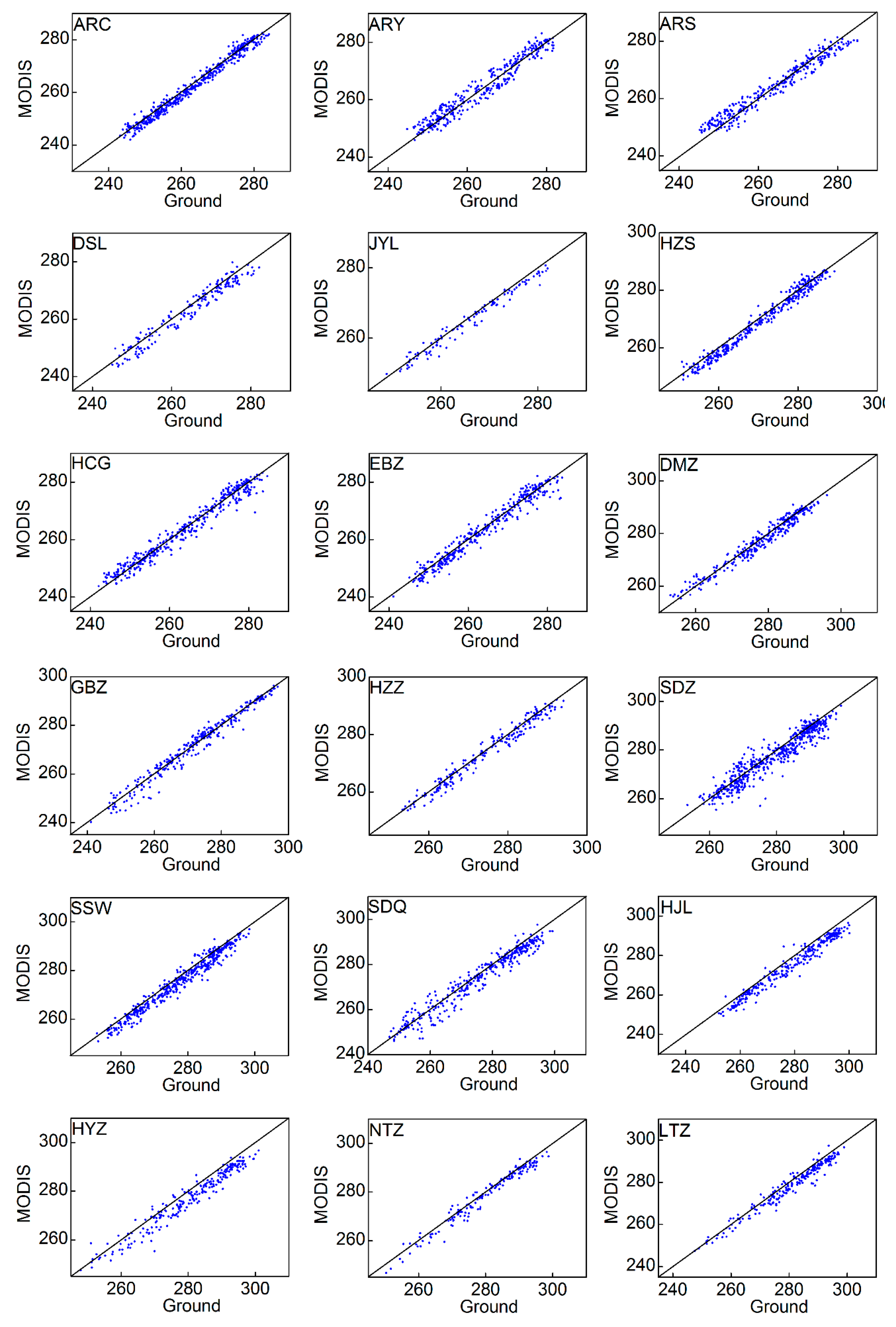
Figure 11.
Relationships between the bias and zenith angle of MODIS when viewing the pixels: (a) relationship during the daytime; and (b) relationship at nighttime.
Figure 11.
Relationships between the bias and zenith angle of MODIS when viewing the pixels: (a) relationship during the daytime; and (b) relationship at nighttime.


Table 1.
Information for the stations in this study.
| Station Name | Longitude/°E | Latitude/°N | Altitude/m | Height/m | Footprint 1/m | Landscapes |
|---|---|---|---|---|---|---|
| A’rou superstation (ARC) | 100.46 | 38.05 | 3033 | 5 | 37.32 | Alpine meadow |
| A’rou sunny slope station (ARS) | 100.52 | 38.09 | 3559 | 6 | 44.78 | Alpine grassland |
| A’rou shade station (ARY) | 100.42 | 37.99 | 3538 | 6 | 44.78 | Alpine grassland |
| Dashalong station (DSL) | 98.95 | 38.83 | 3775 | 6 | 44.78 | Swamp meadow |
| Jinyangling station (JYL) | 101.11 | 37.85 | 3700 | 6 | 44.78 | Alpine meadow |
| Huangzangsi station (HZS) | 100.19 | 38.23 | 2660 | 6 | 44.78 | Cropland (wheat) |
| Huangcaogou station (HCG) | 100.73 | 38.00 | 3186 | 6 | 44.78 | Alpine grassland |
| E’bo station (EBZ) | 100.94 | 37.96 | 3407 | 6 | 44.78 | Alpine grassland |
| Daman superstation (DMZ) | 100.37 | 38.86 | 1519 | 12 | 89.57 | Cropland (maize) |
| Gobi station (GBZ) | 100.30 | 38.89 | 1571 | 6 | 44.78 | Gobi Desert |
| Huazhaizi desert station (HZZ) | 100.32 | 38.77 | 1726 | 2.5 | 18.66 | Desert steppe |
| Wetland station (SDZ) | 100.45 | 38.97 | 1460 | 6 | 44.78 | Wetland |
| Shenshawo desert station (SSW) | 100.49 | 38.79 | 1582 | 6 | 44.78 | Desert |
| Populus forest station (HYZ) | 101.12 | 41.99 | 927 | 24 | 179.14 | Populus forest |
| Cropland station (NTZ) | 101.13 | 42.01 | 919 | 6 | 44.78 | Cropland |
| Barren-land station (LTZ) | 101.13 | 41.99 | 931 | 6 | 44.78 | Bare soil |
| Sidaoqiao station (SDQ) | 101.12 | 41.99 | 935 | 10 | 74.64 | Euphrates poplar olive and Tamarix mixed forest |
| Mixed forest station (HJL) | 101.13 | 41.99 | 929 | 24 | 179.14 | Euphrates poplar olive and Tamarix mixed forest |
1 “Footprint” refers to the diameter of the footprint; “Height” indicates the installation height.
Table 2.
Grading of the spatial representativeness.
| Level | DLCT > 60% | RB < 0.5% | ASS > 1 km | Description |
|---|---|---|---|---|
| 1 | √ | √ | √ | Best representativeness level with strict point-to-pixel LST and LCT value consistency, and a homogeneous LST distribution |
| 2 | √ | √ | × | High representativeness level with high point-to-pixel LST and LCT value consistency but an incomplete homogeneous LST distribution |
| 3 | √ | × | √ | Moderate representativeness level with high LCT consistency and a relatively homogeneous LST distribution but low point-to-area LST consistency |
| 4 | √ | × | × | Low representativeness level with low point-to-area LST consistency and a heterogeneous LST distribution |
| 5 | × | - | - | Minimal representativeness level with various LCTs in pixels and mismatch land-cover observations |
Table 3.
Summary of the statistical comparison results between the MODIS LSTs and the LST measurements from the HiWATER sites.
Table 3.
Summary of the statistical comparison results between the MODIS LSTs and the LST measurements from the HiWATER sites.
| Station | MOD a | MYD b | ||||||
|---|---|---|---|---|---|---|---|---|
| Day | Night | Day | Night | |||||
| Bias | RMSE | Bias | RMSE | Bias | RMSE | Bias | RMSE | |
| ARC | −0.55 | 2.16 | 0.98 | 2.15 | −0.52 | 1.92 | 0.67 | 1.94 |
| ARY | −0.79 | 5.50 | −0.51 | 2.25 | −0.96 | 4.48 | −0.28 | 2.56 |
| ARS | 0.31 | 2.56 | 0.01 | 2.64 | 0.56 | 2.54 | −0.39 | 2.57 |
| DSL | 1.07 | 1.74 | 1.25 | 1.22 | 0.89 | 1.87 | 1.27 | 2.16 |
| JYL | −2.79 | 3.14 | 0.96 | 1.41 | −2.94 | 3.09 | 0.47 | 2.26 |
| HZS | 0.10 | 3.49 | 1.65 | 1.19 | −0.13 | 3.73 | 0.96 | 1.94 |
| HCG | −1.31 | 2.36 | 0.62 | 1.96 | −1.68 | 2.92 | −0.25 | 2.33 |
| EBZ | −0.78 | 2.07 | 0.77 | 1.61 | −0.97 | 2.39 | 0.23 | 2.56 |
| DMZ | −0.88 | 2.81 | 1.23 | 1.45 | −0.96 | 2.77 | 0.21 | 2.21 |
| GBZ | 0.17 | 2.25 | −0.01 | 1.52 | 1.08 | 1.75 | 0.66 | 2.99 |
| HZZ | 0.74 | 1.86 | 0.93 | 1.28 | 0.25 | 2.46 | 0.69 | 2.08 |
| SDZ | −4.12 | 2.93 | 1.90 | 2.74 | −3.44 | 2.71 | 1.26 | 3.78 |
| SSW | 1.34 | 4.18 | 2.49 | 1.60 | 1.57 | 2.95 | 1.55 | 2.51 |
| SDQ | −1.84 | 3.18 | 1.95 | 1.21 | −1.65 | 2.35 | 1.50 | 3.80 |
| HJL | −4.23 | 2.70 | 3.56 | 1.90 | −4.55 | 2.81 | 3.48 | 3.82 |
| HYZ | −0.72 | 5.18 | 3.86 | 2.03 | −0.71 | 5.94 | 2.75 | 3.14 |
| NTZ | −4.72 | 4.08 | 1.43 | 1.47 | −0.17 | 5.44 | 1.15 | 2.91 |
| LTZ | 6.46 | 4.21 | 2.45 | 1.15 | 6.24 | 3.68 | 1.77 | 3.02 |
a The MOD columns show the results of a comparison between the LSTs from the MODIS onboard Terra and the ground-based measurements at the eighteen sites; b The MYD columns show the results of a comparison between the LSTs from the MODIS onboard Aqua and the ground-based measurements at the eighteen sites.
Table 4.
Validation results for MOD/MYD11A1 based on the spatial representativeness levels of the station observations.
Table 4.
Validation results for MOD/MYD11A1 based on the spatial representativeness levels of the station observations.
| Level | MOD a | MYD b | ||||||
|---|---|---|---|---|---|---|---|---|
| Day | Night | Day | Night | |||||
| Bias | RMSE | Bias | RMSE | Bias | RMSE | Bias | RMSE | |
| Level 1 | −0.19 | 1.75 | 0.8 | 1.58 | 0.30 | 1.79 | 0.43 | 1.84 |
| Level 2 | −1.13 | 4.58 | 1.24 | 2.53 | −1.48 | 3.24 | 0.32 | 2.60 |
| Level 3 | 1.45 | 4.93 | 1.44 | 2.23 | 0.47 | 3.67 | 0.77 | 2.67 |
| Level 4 | −2.94 | 5.93 | 2.51 | 3.89 | −2.25 | 4.56 | 1.33 | 4.15 |
| Level 5 | 2.03 | 6.27 | 3.60 | 4.52 | −0.36 | 5.88 | 2.28 | 4.29 |
| All | 0.59 | 4.93 | 2.39 | 3.55 | −0.27 | 4.58 | 1.28 | 3.32 |
a The MOD columns show the results of a comparison between the LSTs from the MODIS onboard Terra and the ground-based measurements at the eighteen sites; b The MYD columns show the results of a comparison between the LSTs from the MODIS onboard Aqua and the ground-based measurements at the eighteen sites.
© 2017 by the authors. Licensee MDPI, Basel, Switzerland. This article is an open access article distributed under the terms and conditions of the Creative Commons Attribution (CC BY) license (http://creativecommons.org/licenses/by/4.0/).
Share and Cite
MDPI and ACS Style
Yu, W.; Ma, M.; Li, Z.; Tan, J.; Wu, A. New Scheme for Validating Remote-Sensing Land Surface Temperature Products with Station Observations. Remote Sens. 2017, 9, 1210. https://doi.org/10.3390/rs9121210
AMA Style
Yu W, Ma M, Li Z, Tan J, Wu A. New Scheme for Validating Remote-Sensing Land Surface Temperature Products with Station Observations. Remote Sensing. 2017; 9(12):1210. https://doi.org/10.3390/rs9121210
Chicago/Turabian StyleYu, Wenping, Mingguo Ma, Zhaoliang Li, Junlei Tan, and Adan Wu. 2017. "New Scheme for Validating Remote-Sensing Land Surface Temperature Products with Station Observations" Remote Sensing 9, no. 12: 1210. https://doi.org/10.3390/rs9121210
Note that from the first issue of 2016, this journal uses article numbers instead of page numbers. See further details here.