Spatiotemporally Representative and Cost-Efficient Sampling Design for Validation Activities in Wanglang Experimental Site


1
Research Center for Digital Mountain and Remote Sensing Application, Institute of Mountain Hazards and Environment, Chinese Academy of Sciences, Chengdu 610041, China
2
CREAF, E08193 Bellaterra (Cerdanyola del Vallès), Catalonia, Spain
*
Author to whom correspondence should be addressed.
Remote Sens. 2017, 9(12), 1217; https://doi.org/10.3390/rs9121217
Submission received: 12 September 2017
/
Revised: 22 November 2017
/
Accepted: 23 November 2017
/
Published: 26 November 2017
(This article belongs to the Special Issue Advances in Quantitative Remote Sensing in China – In Memory of Prof. Xiaowen Li)
Abstract
:Spatiotemporally representative Elementary Sampling Units (ESUs) are required for capturing the temporal variations in surface spatial heterogeneity through field measurements. Since inaccessibility often coexists with heterogeneity, a cost-efficient sampling design is mandatory. We proposed a sampling strategy to generate spatiotemporally representative and cost-efficient ESUs based on the conditioned Latin hypercube sampling scheme. The proposed strategy was constrained by multi-temporal Normalized Difference Vegetation Index (NDVI) imagery, and the ESUs were limited within a sampling feasible region established based on accessibility criteria. A novel criterion based on the Overlapping Area (OA) between the NDVI frequency distribution histogram from the sampled ESUs and that from the entire study area was used to assess the sampling efficiency. A case study in Wanglang National Nature Reserve in China showed that the proposed strategy improves the spatiotemporally representativeness of sampling (mean annual OA = 74.7%) compared to the single-temporally constrained (OA = 68.7%) and the random sampling (OA = 63.1%) strategies. The introduction of the feasible region constraint significantly reduces in-situ labour-intensive characterization necessities at expenses of about 9% loss in the spatiotemporal representativeness of the sampling. Our study will support the validation activities in Wanglang experimental site providing a benchmark for locating the nodes of automatic observation systems (e.g., LAINet) which need a spatially distributed and temporally fixed sampling design.

1. Introduction
Accurate spatiotemporal characterization of land surface heterogeneity [1,2,3] is essential for remote sensing [4] and the land surface [5] modeling. The assumption of surface spatial homogeneity within the Elementary Modeling Unit (EMU) (e.g., a pixel for a remote sensing image or a grid for a land surface model) induces scaling errors [6,7]. This is especially the case for coarse spatial resolution EMU and satellite land surface products with resolutions ranging from 500 m [8] to 5 km [9]. The magnitude of the scaling error is determined by the nonlinearity of the process to be modeled and the surface heterogeneity within the EMU which is often ignored [10,11]. Quantifying the sub-pixel/-grid heterogeneity is the prerequisite for the parameterization, calibration and validation of the remote sensing and the land surface process models [1,12].
Spatiotemporal representative field measurements are required to reproduce the surface heterogeneity within a coarse spatial resolution EMU and to support validation of satellite surface products. However, labour-intensive field measurement collection is usually limited by budget and time constraints. In this sense, the design of efficient sampling strategies preserving the statistics of the population [13,14,15] within an affordable cost is urgently needed.
The Land Product Validation (LPV of the Committee Earth Observing Satellites’ Working Group on Calibration and Validation (CEOS WGCV) recommended a two-stage nested sampling framework to account for the multi-scale nature of the heterogeneity [16]. Fine spatial resolution satellite imagery (about 30 m) are used as a bridge to upscale field measurements to the EMU scale. One of the key points in this framework is the introduction of Elementary Sampling Unit (ESUs) that has approximately the same size as the fine resolution image pixel. Another key point in this framework is the establishment of a transfer function to relate the field measurements over the ESUs with the fine resolution image data. This transfer function can then be used to generate a fine resolution reference map which serves as the benchmark to characterize the surface heterogeneity within the EMU’s coarse spatial resolution. The two-stage nested sampling refers to the sampling of field measurements within the ESU and the sampling of ESUs within the EMU [17]. At ESU scale, square, cross or transect sampling schemes are recommended depending on the measuring instrument and the characteristics of the surface [17]. The sampling scheme at the EMU scale is still far from mature.
The most commonly used sampling strategies at the EMU scale can be categorized into random, systematic, and stratified sampling [18]. Recent researches have increasingly relied on the stratified sampling based on a priori information. Stratified sampling strategies firstly select auxiliary variables which can be easily generated from remote sensing observations (vegetation indices, generally) to represent the target variables (e.g., leaf area index, fractional vegetation cover and chlorophyll content), then subdivide each auxiliary variable into several strata, and finally sample the plots randomly within each stratum. Stratified sampling strategies are assumed to be capable of optimally capturing the variability across the site extent [13,19,20,21]. The conditioned Latin hypercube (CLH) sampling is among the most appealing stratified sampling strategies [22]. CLH was proposed in the context of digital soil mapping, but has been used in many other fields because of its representativeness and extensibility [22,23,24]. Recently, Zeng et al. [25] and Yin et al. [14] introduced this method to the ESU sampling.
Existing researches on field sampling design generally focused on capturing the landscape spatial heterogeneity by distributing the ESUs across the entire study area [16,18,19,20,21]. Two key issues, which are the main scientific questions addressed in this paper, were often ignored in traditional ESU sampling schemes: First, the spatial heterogeneity changes over time. Second, some parts of the study area may be inaccessible because of the rugged terrain, lack of roads or barrier of river. Addressing the temporal dynamics of the surface spatial [26,27] is key for the development of the near-surface remote sensing technologies which can provide long-term measurements automatically [28,29,30]. Zeng et al. [25] employed multi-temporal vegetation index maps as a priori information to constrain the sampling process and generate spatiotemporally representative ESUs. However, the accessibility of the sampling plots was neglected in this scheme [25] which may be critical in traffic inconvenient regions. In fact, the cost limitation in field campaign was already considered by few previous studies. Yin et al. [14] incorporated a cost-objective function to traditional CLH to define a cost-efficient sampling design. However, some inaccessible ESUs may remain in this sampling scheme, which is based on a global minimization of the cost-objective function. In addition, the temporal variation of the spatial heterogeneity was not considered. To summarize, the spatiotemporally heterogeneity and cost limitation were separately accounted for by [14] and [25], respectively. However, an integrated approach for defining an optimal sampling design capturing the land surface spatiotemporally heterogeneity in a cost-efficient way is still urgently needed. This sampling design is especially important for mountainous areas which are characterized both by extreme heterogeneity and inaccessibility.
The Wanglang Integrated Observation and Experiment Station for Mountain Ecological Remote Sensing was recently established in the Wanglang Nature Reserve, one of China’s first nature reserves established to protect the giant panda in 1965. Temporally continuous field measurements of biophysical variables (including leaf area index, fractional vegetation cover, fraction of absorbed photosynthetically active radiation) are planned to be implemented in 2018 to support the parameterization, calibration and validation of the remote sensing and the land surface process models. Establishing an optimized sampling design to generate spatiotemporally representative and cost-efficient ESUs is the prerequisite for the planned measurements in Wanglang experimental site and the main objective of this paper.
2. Study Site
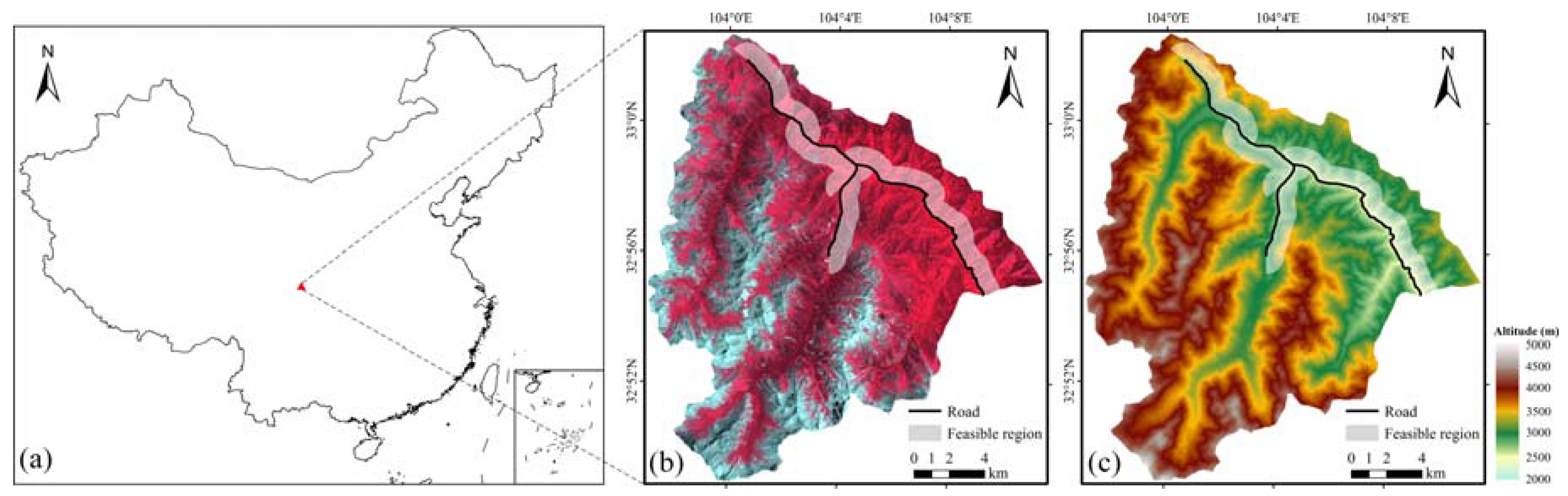
The Wanglang Nature Reserve (Figure 1) is located in the Hengduan Mountains, a global biodiversity hotspot. The reserve covers approximately 320 km2 with altitudes ranging between 2000 and 5000 m (Figure 1c). It receives 862.5 mm of rainfall annually, with the lowest mean air temperature of −6.1 °C in January, and the highest at 12.7 °C in July [31]. The major vegetation types include deciduous forest, conifer-deciduous mixed forest, and conifer forest. The transportation is inconvenient with the roads built along rivers (Figure 1b). Most of the parts in the reserve are difficult or even impossible to visit.
Based on the reserve, the Wanglang Integrated Observation and Experiment Station for Mountain Ecological Remote Sensing was established in 2017. One of the scientific objective of this station is to implement temporally continuous validation for existing remote sensing products. To complete this objective, temporally continuous field measurements are planned to be implemented in 2018. Wireless sensor network system, which needs the support of permanent ESUs [25], is an efficient means to collect these temporally continuous field measurements [28,30].
3. Materials and Methods
3.1. Auxiliary Satellite Imagery
We used Normalized Difference Vegetation Index (NDVI) [32] as the auxiliary variable to represent the target biophysical properties. NDVI has been demonstrated to show a strong correlation with many biophysical variables including leaf area index (LAI) [11,33], fraction of absorbed photosynthetically active radiation (FAPAR) [34,35], and fraction of vegetation cover (FVC) [36,37]. In addition, the NDVI reduces the sensitive to topographic effects due to its ratio formulation [38,39].
NDVI maps of the study area were here computed from Landsat top of canopy reflectance data in the near infrared and red bands. Landsat data were downloaded from the United States Geological Survey (USGS) EarthExplorer (https://earthexplorer.usgs.gov/) [40]. The Landsat reflectance data were atmospherically corrected using the Second Simulation of the Satellite Signal in the Solar Spectrum-Vector (6SV) model [41].
To capture the seasonal variations of the vegetation, we collected five scenes of images spanning nearly the whole growing season peak in our study area: Day of Year (DOY) 152, 197, 240, 261, 296. Because of the cloud contamination, no single year can provide cloud-free images covering the whole growing season peak. The five selected scenes were from different years and sensors (Table 1). This treatment neglected the inter-annual variation of vegetation and the difference in spectral response function between Landsat 8/OLI and Landsat 5/TM.
3.2. Definition of the Sampling Feasible Region
The study area is characterized by inaccessibility because of the rugged terrain, lack of roads and barrier of river. Therefore, we should consider the cost limitation when determining the spatial distribution of the ESUs. Different from Silva et al. [24] and Yin et al. [14], who calculated the visiting cost for each pixel and incorporated a cost-objective function to constrain the sampling process, in this paper, we first established the feasible region for the ESU sampling within an affordable cost. The establishment of feasible region avoid the generation of unaffordable ESUs located in inaccessible regions, which is a potential problem of the methods of Silva et al. [24] and Yin et al. [14].
The feasible region (Figure 1) is defined according to two practical criteria:
- The distance between the ESUs and the roads should be less than 1000 m.
- The ESUs and the roads should be on the same side of the rivers.
The criterion I considers the influence of the rugged terrain and lack of roads. Note that the distance threshold of 1000 m was set according to expert experiences, and it directly influence the cost and the spatiotemporal representativeness of the sampled ESUs. The criterion II considers the block of rivers. The roads in our study area are often built along the rivers, so the ESUs and the roads should be on the same side of the rivers to avoid crossing rivers.
3.3. Multi-Temporal Constraint Sampling Based on the Conditioned Latin Hypercube (CLH)
The proposed sampling scheme aims to obtain representative samples and reproduce the probability distribution functions of the five NDVI maps (Table 1) using n spatially-distributed and temporally-fixed ESUs. It is based on the CLH sampling procedure [22] and iteratively selects samples from the NDVI maps by using a stratified random sampling scheme based on the cumulative distributions of NDVI. CLH is implemented by the following steps:
- Divide the probability distributions of NDVI for the five dates into n equiprobable strata.
- Randomly pick one sample (ESU) per stratum. The location of the ESUs is constrained within the feasible region (Figure 1).
- The objective function is defined as follows:where n is the number of ESUs, k is the number of NDVI maps (k = 5, in this study), ηij is the times that a stratum i on date j is sampled.
- Perform an annealing schedule [42] to minimize the objective function. To avoid being trapped in a local optimum, the simulated annealing algorithm accepts some of the changes that worsen the objective function, and the probability of accepting a worse sample is given by:where ΔO is the change in the objective function and T is a control parameter for optimizing the global minimization of the objective function O. For each T value (between 0 and 1) there is a corresponding probability p to get out of a local minimum in the minimization procedure. The greater of T, the higher probability to get out of a local minimum, but with more computation time, and vice versa. We fixed the initial value of T to 1 and it was decreased by a factor 0.95 during each iteration.
- Perform the replacement of an ESU in the selected sample with an ESU outside the current sample. The replacement can be random or systematic, according to a probability of F. Specifically, generate a random number rand, if rand < F, pick a ESU randomly from currently generated sample (random replacement) and swap it with a random ESU outside the current sample. Otherwise, remove the ESU from current sample which has the largest overall objective function value (systematic replacement), and replace it with a random ESU outside the current sample. The value of F was fixed to 0.5 using a trial-and-error approach.
- Repeat steps III–V a number of 5000 iterations to converge to the final solution.
3.4. Evaluation Approach
Similar to the VALERI’s sampling protocol [17], the size of the ESUs corresponds to the size of the pixel of the high spatial resolution satellite data, i.e., the 30 m of Landsat data in our case. The NDVI values for each ESU and for the different dates were extracted from the five Landsat NDVI maps (Table 1). To quantitatively evaluate the capacity of the multi-temporally constrained (MC) sampling strategy for reproducing the NDVI values across the study area and for the different dates, we computed the Overlapping Area (OA) between the NDVI frequency distribution histogram from the ESUs (denoted by Fs) and that from the entire study area (denoted by Fp) considering the NDVI values of all the different dates. The OA can be formulated as [43],
The numerator denotes the overlapping area of Fs and Fp, and the denominator represents the area of Fp.
R2 and root mean square error (RMSE) between the mean NDVI values from the ESUs and the average values for the entire study area for each date were also computed to quantify if resulting ESUs can preserve the average state of the study area.
The proposed multi-temporally constrained (MC) sampling was compared with two alternative sampling schemes: the single-temporally constrained (SC) sampling that uses only one NDVI map (DOY 197) to construct the objective function (Equation (1)) and the random sampling (RS) without addition constraints. Similarly to MC, the distribution of samples for the SC and RS schemes were limited to the feasible region. Finally, a multi-temporally constrained sampling with ESUs located across the entire study area (MCE) was used for evaluating the theoretical impact in terms of spatiotemporal representativeness of introducing a feasible region for the cost limitation. Note however that the MCE sampling design is unaffordable in the practice due to the inaccessibility of some of the ESUs.
4. Results
4.1. Influence of the Number of Elementary Sampling Units in the Spatiotemporal Representativeness
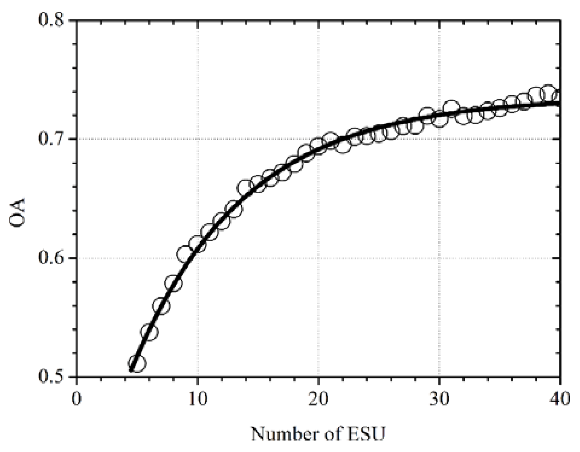
To determine the minimum number of ESUs required to capture the spatiotemporal heterogeneity of the study area, we analyzed the variations of the mean OA of the five dates as a function of the number of ESUs (Figure 2). The OA increases with the number of ESUs indicating, as expected, that the spatiotemporal heterogeneity of the study area can be better represented with a higher number of ESUs. The OA can be well fitted (R2 = 0.99) by an exponential function:
where n is the number of ESUs. For low n values, the OA increased rapidly with n. For high n values, the OA reaches an asymptotic value of 0.74. For n = 20 samples, 70% of the heterogeneity of the study area is well represented. This cut-off point of n = 20 was fixed as the minimum required number of ESUs.
OA = 0.74 − 0.37exp(−0.11n)
Note that about 25% of the spatiotemporal heterogeneity cannot be represented by the MC sampling scheme (Figure 2). This may be partially explained because the samples were located in a feasible region significantly smaller than the entire study area and may not completely cover all the range of vegetation conditions (Figure 3).
Figure 3 shows the spatial distribution of the 20 selected ESUs by the multi-temporal and cost constrained sampling strategy within the pre-defined sampling feasible region.
4.2. Performance Evaluation: Comparison with Alternative Sampling Designs
Figure 4 shows the NDVI frequency distribution histograms of the 20 selected ESUs for the four sampling strategies: random sampling (RS), single-temporally constrained sampling (SC), and multi-temporally constrained sampling both in the feasible region (MC) and in the entire study area without the sampling feasible constraint (MCE).
The MCE sampling strategy performed the best and reconstructed the NDVI frequency distribution histograms of the entire study area for the different dates more accurately than the feasible region constrained sampling designs. The introduction of sampling feasible region slightly degreased the spatiotemporal representativeness of sampling but, in general, the three methods RS, SC and MC applied for the feasible region can all preserve the overall shapes of the frequency distribution histograms of the entire study area (red lines in Figure 4), with the MC performing the best. On DOY 152, RS under-sampled the interval 0.4–0.65 and over-sampled the NDVI interval 0.8–0.85. On DOY 261, RS and SC both under-sampled the NDVI intervals less than 0.6. On DOY 197, all methods significantly over-sampled high NDVI values for the range 0.85–0.9.
The comparison of the OA for the four sampling strategies (Table 2) showed that MCE performed the best during the whole study period (OA = 83.5%) followed by MC (OA = 74.7%). RS performed the worst (OA = 63.1%) because it exploited no a priori information. The efficiency of SC was between RS and MC (OA = 68.7%), but it improved the spatiotemporal representativeness for DOY 197 (OA = 75.9%) because this specific date was used to constrain the SC sampling procedure.
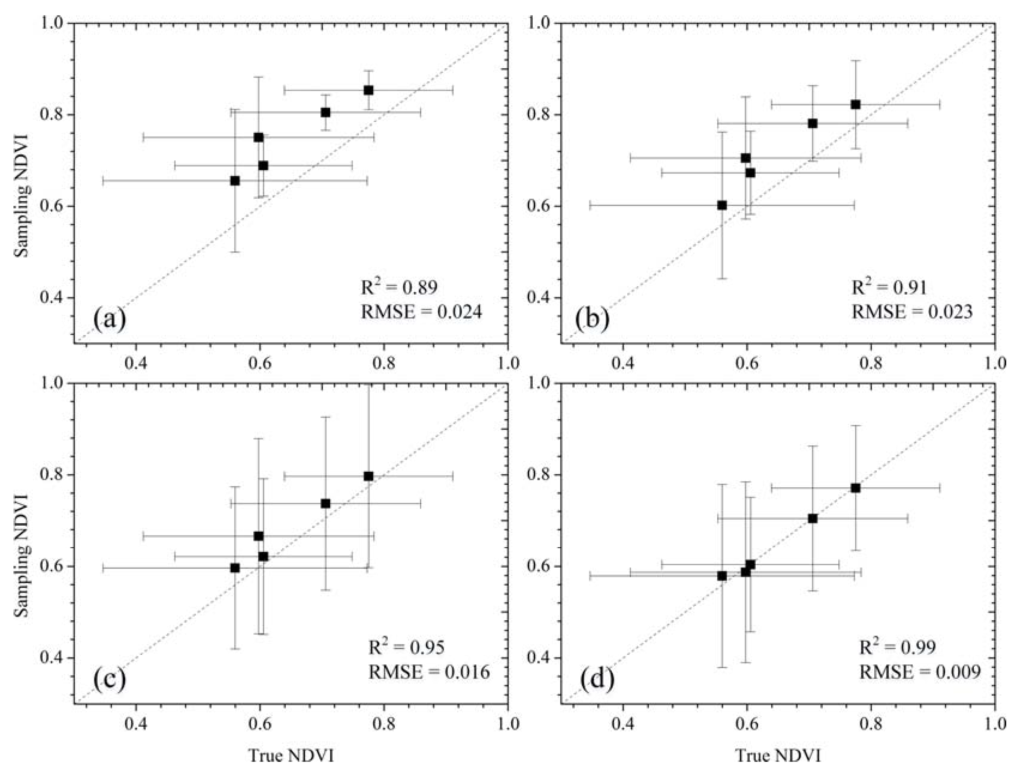
The scatterplots between the average of sampled NDVI and the average NDVI calculated from the whole study area were also analyzed (Figure 5). The MCE method was the most accurate (RMSE < 0.01) for NDVI sampling (R2 = 0.99). The three sampling strategies constrained to the feasible region all overestimated the regional means. The feasible region is located in the lowland areas which generally have better hydrologic and thermal conditions than highland areas for vegetation growth. Compared to the RS and SC, MC sampling significantly alleviated the overestimation phenomenon.
The reduction of standard deviation from the ESUs compared to that from the entire study area indicates the information loss on spatiotemporal heterogeneity [12]. Figure 5 shows that the RS had the smallest standard deviation for each DOY, followed by SC and MC. MCE and MC show similar variability in terms of the standard deviation. This demonstrates the efficiency of CLH strategy for defining spatiotemporal representativeness sampling schemes.
5. Discussion
This study proposed a novel sampling strategy to generate spatiotemporally representative and cost-efficient ESUs. Comparing to existing study about ESU sampling methods [14,20,25], our method can make an appropriate compromise between spatiotemporal representativeness and implementation cost, so it is particularly useful for heterogenous and traffic-inconvenient regions, e.g., mountainous regions.
The multi-temporal constrained sampling was demonstrated to better capture the spatiotemporal surface heterogeneity compared to random or single-temporal constrained methods. The introduction of the feasible region (Figure 1) reduced about 9% the spatiotemporal representativeness of the multi-temporal constrained sampling based on CLH (compare MC and MCE in Figure 4 and Table 2). The feasible region is located in lowland areas with high NDVI values and may not completely represent all the range of conditions of vegetation in the entire mountainous region, which is characterized by a vertical negative gradient in NDVI (Figure 5). However, the feasible region was established based on accessibility criteria and the spatial distribution of the available roads in the study area. The loss of information of the feasible constrained sampling (MC) is compensated by the significant reduction of the implementation cost.
A sensitivity analysis showed that 20 ESUs can reproduce 70% of heterogeneity of the study area. The distribution of the 20 selected ESUs within the pre-defined feasible region showed some spatial aggregation (Figure 3). This phenomenon was often criticized for information redundancy because of the spatial autocorrelation of the biophysical condition [44]. Although this aggregation of ESUs could be easily removed by introducing additional objective function in geographic space [14,21,25], the cluster of the ESUs would allow reducing the implementation cost of the field campaigns which is one of the key concerns of the present study.
A spatially-distributed and temporally-fixed strategy for the ESU sampling was adopted in this study. Alternatively, a temporally independent strategy could be adopted for defining the ESU sampling for multi-temporal field campaigns, i.e., different date uses different spatial distribution of ESUs. The temporally independent manner may show better capacity to capture the temporal variation of spatial heterogeneity. However, the temporally-fixed manner can provide additional information of the temporal variation of vegetation at each ESU. The temporally-fixed strategy was here selected because it allows locating the nodes of the wireless sensor network systems that will support the validation activities in Wanglang experimental site [19,25,28].
To consider the rugged terrain, lack of roads and the block of rivers, we restricted the ESUs within the sampling feasible region. Currently, the feasible region was established in a semi-empirical manner based on our expert knowledge. Some more sophisticate algorithms (e.g., three-dimensional terrain modeling, 3D analyzing and the shortest path algorithm) would enhance the rationality in the definition of the feasible region.
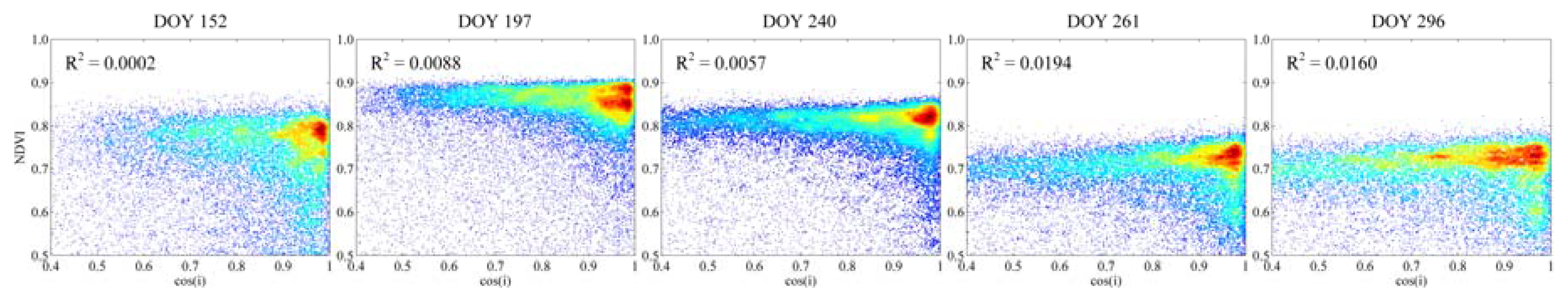
In this study, NDVI was chosen to represent the biophysical properties of the study area. One reason to select NDVI is because of its strong correlation with many biophysical variables. Although other vegetation indices such as the soil adjusted vegetation index [45], the enhanced vegetation index [46], the normalized difference water index [47] or the normalized canopy index [48] were also recommended in some specified applications, they were often criticized for their vulnerability to topographic effects [39]. Figure 6 showed the density scatterplots between the NDVI and the cosine of the local solar incidence (cos(i)) in our study area, which is the most widely used quantitative evaluation method for topographic effects [49]. It can be seen that NDVI was nearly independent from cos(i) with R2 between them ranging from 0.0002 to 0.0194. NDVI was then selected as the auxiliary variable for our sampling procedure due to its correlation with many biophysical variables and its reduced sensibility to topographic effects.
The topography is well recognized to influence the vegetation biophysical properties [50,51]. Topographical factors (e.g., slope) were introduced as auxiliary variables in our previous study [14]. However, the NDVI relates to biophysical properties more explicitly. The exclusion of topography would not limit the representativeness of the sampled ESU considering the low sensibility of NDVI to topographic effects for the study area and considered period.
The use of NDVI data from different sensor and years may introduce uncertainties in the sampling procedure. However, our study area is a natural reserve where the anthropogenic activities (e.g., logging and mining) are very limited and, consequently, induced rapid changes in biophysical properties are not expected. Moreover, the study area is dominated by primeval forest with mean age around 200 years and significant inter-annual variations in vegetation are not expected for the period of the satellite acquisitions (Table 1). In our conditions, the NDVI data from different years is expected to successfully represent the seasonal variations in surface heterogeneity. In addition, it was demonstrated in a few studies that the Landsat data record shows satisfactory consistency, and can be safely used together for time series analysis [52,53]. Therefore, the combined use of Landsat 8/OLI and Landsat 5/TM is also acceptable in the sampling procedure. An alternative to capture the seasonal variations is the combination of Landsat 8 with Sentinel-2 images. However, the persistent cloud cover during the monsoon (from July to September) hampers the collection of clear Sentinel-2 images in our study area. Moreover, cross-calibration coefficients between Landsat 8 with Sentinel-2 retrieved from pseudo-invariant sites [54] may be not suitable for mountainous areas. The footprints of sensor observations vary considerably in size and center locations over time, which hamper the establishment of robust cross-calibration coefficients [55]. This also prevents the normalization between Landsat 8/OLI and Landsat 5/TM data over reference targets.
According to the protocols established by the LPV subgroup [16] and the VALERI project [17], each ESU corresponds to a pixel of the auxiliary high spatial resolution satellite data. In this study, the size of each ESU is 30 m × 30 m corresponding to the spatial resolution of the OLI images. As recommended by the two-stage nested sampling framework [16], a sampling procedure would also be implement within each ESU by distributing the individual field measurements in squares, crosses or transects [17]. The specified sampling design within each ESU is out of the scope of this study.
Because of the lack of in-situ measurements, the sampling strategies were evaluated through the comparison of the sampled and true NDVI frequency distributions. The sampling strategies will be further evaluated using the in-situ measurements that will be collected in the Wanglang field campaigns planned for the year 2018.
6. Conclusions
We proposed a sampling strategy to generate spatiotemporally representative and cost-efficient ESUs based on the conditioned Latin hypercube methodology. The proposed sampling strategy was constrained by multi-temporal NDVI, and the ESUs were limited within a feasible region established based on accessibility criteria. A case study in Wanglang National Nature Reserve in China showed that the proposed strategy can obtain more spatiotemporally representative ESUs (mean annual Overlapping Area, OA = 74.7%), compared to the single-temporally constrained (OA = 68.7%) and random sampling (OA = 63.1%) strategies. The minimum number of required ESUs was fixed to twenty as a compromise between the spatiotemporal representativeness and the implementation cost. The introduction of the feasible region constraint ensures an affordable cost for the field campaigns at expenses of a degradation of about 9% in the spatiotemporal representativeness of the sampling. The sampling design here proposed will support validation activities in Wanglang experimental site providing a benchmark of spatially distributed and temporally fixed ESUs for locating the nodes of wireless sensor network systems for the acquisition of temporally continuous field measurements.
Acknowledgments
This work was funded by the National Key Research and Development Program of China (2016YFA0600103), the National Natural Science Foundation of China (41601403, 41631180, 41571373, and 41531174), by the Youth Talent Team Program of Institute of Mountain Hazards and Environment, Chinese Academy of Sciences under Grant SDSQB-2015-02, and by the CAS “Light of West China” Program. A.V. acknowledges the support from the EC Copernicus Global Land Service (CGLOPS-1, 199494-JRC).
Author Contributions
Ainong Li conceived the experiments; Gaofei Yin designed and performed the experiments, and wrote the paper; Aleixandre Verger provided guidance and critically reviewed the manuscript.
Conflicts of Interest
The authors declare no conflict of interest.
References
- Li, X. Characterization, controlling, and reduction of uncertainties in the modeling and observation of land-surface systems. Sci. China Earth Sci. 2014, 57, 80–87. [Google Scholar] [CrossRef]
- Li, X.; Cheng, G.D.; Liu, S.M.; Xiao, Q.; Ma, M.G.; Jin, R.; Che, T.; Liu, Q.H.; Wang, W.Z.; Qi, Y.; et al. Heihe Watershed Allied Telemetry Experimental Research (HiWATER): Scientific objectives and experimental design. Bull. Am. Meteorol. Soc. 2013, 94, 1145–1160. [Google Scholar] [CrossRef]
- Xu, B.D.; Li, J.; Liu, Q.H.; Huete, A.R.; Yu, Q.; Zeng, Y.L.; Yin, G.F.; Zhao, J.; Yang, L. Evaluating spatial representativeness of station observations for remotely sensed leaf area index products. IEEE J. Sel. Top. App. Earth Obs. Remote Sens. 2016, 9, 3267–3282. [Google Scholar] [CrossRef]
- Verhoef, W.; Bach, H. Coupled soil-leaf-canopy and atmosphere radiative transfier modeling to simulate hyperspectral multi-angular surface reflectance and TOA radiance data. Remote Sens. Environ. 2007, 109, 166–182. [Google Scholar] [CrossRef]
- Kure, S.; Kavvas, M.L.; Ohara, N.; Jang, S. Upscaling of coupled land surface process modeling for heterogeneous landscapes: Stochastic approach. J. Hydrol. Eng. 2011, 16, 1017–1029. [Google Scholar] [CrossRef]
- Li, X.; Wang, Y. Prospects on future developments of quantitative remote sensing. Acta Geogr. Sin. 2013, 68, 1163–1169. [Google Scholar]
- Yan, G.J.; Hu, R.H.; Wang, Y.T.; Ren, H.Z.; Song, W.J.; Qi, J.B.; Chen, L. Scale effect in indirect measurement of leaf area index. IEEE Trans. Geosci. Remote Sens. 2016, 54, 3475–3484. [Google Scholar] [CrossRef]
- Yan, K.; Park, T.; Yan, G.J.; Chen, C.; Yang, B.; Liu, Z.; Nemani, R.R.; Knyazikhin, Y.; Myneni, R.B. Evaluation of MODIS LAI/FPAR product collection 6. Part 1: Consistency and improvements. Remote Sens. 2016, 8, 359. [Google Scholar] [CrossRef]
- Claverie, M.; Matthews, J.L.; Vermote, E.F.; Justice, C.O. A 30+ year AVHRR LAI and FAPAR climate data record: Algorithm description and validation. Remote Sens. 2016, 8, 263. [Google Scholar] [CrossRef]
- Wu, H.; Li, Z.L. Scale issues in remote sensing: A review on analysis, processing and modeling. Sensors 2009, 9, 1768–1793. [Google Scholar] [CrossRef] [PubMed]
- Yin, G.F.; Li, J.; Liu, Q.H.; Li, L.H.; Zeng, Y.L.; Xu, B.D.; Yang, L.; Zhao, J. Improving leaf area index retrieval over heterogeneous surface by integrating textural and contextual information: A case study in the Heihe River Basin. IEEE Geosci. Remote Sens. Lett. 2015, 12, 359–363. [Google Scholar]
- Garrigues, S.; Allard, D.; Baret, F.; Weiss, M. Influence of landscape spatial heterogeneity on the non-linear estimation of leaf area index from moderate spatial resolution remote sensing data. Remote Sens. Environ. 2006, 105, 286–298. [Google Scholar] [CrossRef]
- Grafstrom, A.; Schelin, L. How to select representative samples. Scand. J. Stat. 2014, 41, 277–290. [Google Scholar] [CrossRef]
- Yin, G.F.; Li, A.N.; Zeng, Y.L.; Xu, B.D.; Zhao, W.; Nan, X.; Jin, H.A.; Bian, J.H. A cost-constrained sampling strategy in support of LAI product validation in mountainous areas. Remote Sens. 2016, 8, 704. [Google Scholar] [CrossRef]
- Wang, J.F.; Stein, A.; Gao, B.B.; Ge, Y. A review of spatial sampling. Spat. Stat. 2012, 2, 1–14. [Google Scholar] [CrossRef]
- Morisette, J.T.; Baret, F.; Privette, J.L.; Myneni, R.B.; Nickeson, J.E.; Garrigues, S.; Shabanov, N.V.; Weiss, M.; Fernandes, R.A.; Leblanc, S.G.; et al. Validation of global moderate-resolution LAI products: A framework proposed within the CEOS Land Product Validation subgroup. IEEE Trans. Geosci. Remote Sens. 2006, 44, 1804–1817. [Google Scholar] [CrossRef]
- Baret, F.; Weiss, M.; Allard, D.; Garrigue, S.; Leroy, M.; Jeanjean, H.; Fernandes, R.; Myneni, R.; Privette, J.; Morisette, J.; et al. VALERI: A Network of Sites and a Methodology for the Validation of Medium Spatial Resolution Land Satellite Products. Available online: http://w3.avignon.inra.fr/valeri/ (accessed on 24 November 2017).
- Martinez, B.; Garcia-Haro, F.J.; Camacho-de Coca, F. Derivation of high-resolution leaf area index maps in support of validation activities: Application to the cropland Barrax site. Agric. For. Meteorol. 2009, 149, 130–145. [Google Scholar] [CrossRef]
- Ge, Y.; Wang, J.H.; Heuvelink, G.B.M.; Jin, R.; Li, X.; Wang, J.F. Sampling design optimization of a wireless sensor network for monitoring ecohydrological processes in the Babao River basin, China. Int. J. Geogr. Inf. Sci. 2015, 29, 92–110. [Google Scholar] [CrossRef]
- Mu, X.; Hu, M.; Song, W.; Ruan, G.; Ge, Y.; Wang, J.; Huang, S.; Yan, G. Evaluation of sampling methods for validation of remotely sensed fractional vegetation cover. Remote Sens. 2015, 7, 16164–16182. [Google Scholar] [CrossRef]
- Zeng, Y.L.; Li, J.; Liu, Q.H.; Li, L.H.; Xu, B.D.; Yin, G.F.; Peng, J.J. A sampling strategy for remotely sensed LAI product validation over heterogeneous land surfaces. IEEE J. Sel. Top. Appl. Earth Obs. Remote Sens. 2014, 7, 3128–3142. [Google Scholar] [CrossRef]
- Minasny, B.; McBratney, A.B. A conditioned Latin hypercube method for sampling in the presence of ancillary information. Comput. Geosci. 2006, 32, 1378–1388. [Google Scholar] [CrossRef]
- Mulder, V.L.; De Bruin, S.; Schaepman, M.E. Representing major soil variability at regional scale by constrained Latin Hypercube Sampling of remote sensing data. Int. J. Appl. Earth Obs. Geoinf. 2013, 21, 301–310. [Google Scholar] [CrossRef]
- Silva, S.H.G.; Owens, P.R.; Silva, B.M.; De Oliveira, G.C.; De Menezes, M.D.; Pinto, L.C.; Curi, N. Evaluation of conditioned Latin hypercube sampling as a support for soil mapping and spatial variability of soil properties. Soil Sci. Soc. Am. J. 2015, 79, 603–611. [Google Scholar] [CrossRef]
- Zeng, Y.L.; Li, J.; Liu, Q.H.; Qu, Y.H.; Huete, A.R.; Xu, B.D.; Yin, G.F.; Zhao, J. An optimal sampling design for observing and validating long-term leaf area index with temporal variations in spatial heterogeneities. Remote Sens. 2015, 7, 1300–1319. [Google Scholar] [CrossRef]
- Ding, Y.L.; Zhao, K.; Zheng, X.M.; Jiang, T. Temporal dynamics of spatial heterogeneity over cropland quantified by time-series NDVI, near infrared and red reflectance of Landsat 8 OLI imagery. Int. J. Appl. Earth Obs. Geoinf. 2014, 30, 139–145. [Google Scholar] [CrossRef]
- Garrigues, S.; Allard, D.; Baret, F. Modeling temporal changes in surface spatial heterogeneity over an agricultural site. Remote Sens. Environ. 2008, 112, 588–602. [Google Scholar] [CrossRef]
- Qu, Y.H.; Han, W.C.; Fu, L.Z.; Li, C.R.; Song, J.L.; Zhou, H.M.; Bo, Y.C.; Wang, J.D. LAINet—A wireless sensor network for coniferous forest leaf area index measurement: Design, algorithm and validation. Comput. Electron. Agric. 2014, 108, 200–208. [Google Scholar] [CrossRef]
- Ryu, Y.; Lee, G.; Jeon, S.; Song, Y.; Kimm, H. Monitoring multi-layer canopy spring phenology of temperate deciduous and evergreen forests using low-cost spectral sensors. Remote Sens. Environ. 2014, 149, 227–238. [Google Scholar] [CrossRef]
- Yin, G.F.; Li, A.N.; Jin, H.A.; Zhao, W.; Bian, J.H.; Qu, Y.H.; Zeng, Y.L.; Xu, B.D. Derivation of temporally continuous LAI reference maps through combining the LAINet observation system with CACAO. Agric. For. Meteorol. 2017, 233, 209–221. [Google Scholar] [CrossRef]
- Kang, D.W.; Yang, H.W.; Li, J.Q.; Chen, Y.P.; Zhao, L.J. Habitat use by giant pandas Ailuropoda melanoleuca in the Wanglang Nature Reserve, Sichuan, China. Zool. Stud. 2013, 52, 6. [Google Scholar] [CrossRef]
- Huete, A.; Didan, K.; Miura, T.; Rodriguez, E.P.; Gao, X.; Ferreira, L.G. Overview of the radiometric and biophysical performance of the MODIS vegetation indices. Remote Sens. Environ. 2002, 83, 195–213. [Google Scholar] [CrossRef]
- Baret, F.; Guyot, G.; Major, D.J. Crop biomass evaluation using radiometric measurements. Photogrammetria 1989, 43, 241–256. [Google Scholar] [CrossRef]
- Baret, F.; Guyot, G. Potentials and limits of vegetation indexes for LAI and APAR assessment. Remote Sens. Environ. 1991, 35, 161–173. [Google Scholar] [CrossRef]
- Myneni, R.B.; Williams, D.L. On the relationship between FAPAR and NDVI. Remote Sens. Environ. 1994, 49, 200–211. [Google Scholar] [CrossRef]
- Gutman, G.; Ignatov, A. The derivation of the green vegetation fraction from NOAA/AVHRR data for use in numerical weather prediction models. Int. J. Remote Sens. 1998, 19, 1533–1543. [Google Scholar] [CrossRef]
- Yang, G.; Pu, R.; Zhang, J.; Zhao, C.; Feng, H.; Wang, J. Remote sensing of seasonal variability of fractional vegetation cover and its object-based spatial pattern analysis over mountain areas. ISPRS J. Photogramm. Remote Sens. 2013, 77, 79–93. [Google Scholar] [CrossRef]
- Valeriano, M.D.M.; Sanches, I.D.A.; Formaggio, A.R. Topographic effect on spectral vegetation indices from Landsat TM data: Is topographic correction necessary? Bol. Ciências Geodésicas 2016, 22, 95–107. [Google Scholar]
- Zhu, G.; Liu, Y.; Ju, W.; Chen, J. Evaluation of topographic effects on four commonly used vegetation indices. J. Remote Sens. 2013, 17, 210–234. [Google Scholar]
- EarthExplorer. Available online: https://earthexplorer.usgs.gov/ (accessed on 24 November 2017).
- Vermote, E.; Justice, C.; Claverie, M.; Franch, B. Preliminary analysis of the performance of the Landsat 8/OLI land surface reflectance product. Remote Sens. Environ. 2016, 185, 46–56. [Google Scholar] [CrossRef]
- Press, W.H.; Teukolsky, S.A.; Flannery, B.P.; Vetterling, W.T. Numerical Recipes in FORTRAN: The Art of Scientific Computing; Cambridge University Press: Cambridge, UK, 1992. [Google Scholar]
- Jin, H.A.; Li, A.N.; Wang, J.D.; Bo, Y.C. Improvement of spatially and temporally continuous crop leaf area index by integration of CERES-Maize model and MODIS data. Eur. J. Agron. 2016, 78, 1–12. [Google Scholar] [CrossRef]
- Wang, J.F.; Christakos, G.; Hu, M.G. Modeling spatial means of surfaces with stratified nonhomogeneity. IEEE Trans. Geosci. Remote Sens. 2009, 47, 4167–4174. [Google Scholar] [CrossRef]
- Qi, J.; Chehbouni, A.; Huete, A.R.; Kerr, Y.H.; Sorooshian, S. A modified soil adjusted vegetation index. Remote Sens. Environ. 1994, 48, 119–126. [Google Scholar] [CrossRef]
- Jiang, Z.Y.; Huete, A.R.; Didan, K.; Miura, T. Development of a two-band enhanced vegetation index without a blue band. Remote Sens. Environ. 2008, 112, 3833–3845. [Google Scholar] [CrossRef]
- Gao, B.C. NDWI—A normalized difference water index for remote sensing of vegetation liquid water from space. Remote Sens. Environ. 1996, 58, 257–266. [Google Scholar] [CrossRef]
- Vescovo, L.; Gianelle, D. Using the MIR bands in vegetation indices for the estimation of grassland biophysical parameters from satellite remote sensing in the Alps region of Trentino (Italy). Adv. Space Res. 2008, 41, 1764–1772. [Google Scholar] [CrossRef]
- Sola, I.; Gonzalez-Audicana, M.; Alvarez-Mozos, J. Multi-criteria evaluation of topographic correction methods. Remote Sens. Environ. 2016, 184, 247–262. [Google Scholar] [CrossRef]
- Davis, F.W.; Schimel, D.S.; Friedl, M.A.; Michaelsen, J.C.; Kittel, T.G.F.; Dubayah, R.; Dozier, J. Covariance of biophysical data with digital topographic and land-use maps over the FIFE site. J. Geophys. Res. Atmos. 1992, 97, 19009–19021. [Google Scholar] [CrossRef]
- Shen, L.; Li, Z.; Guo, X. Remote sensing of leaf area index (LAI) and a spatiotemporally parameterized model for mixed grasslands. Int. J. Appl. Sci. Technol. 2014, 4, 46–61. [Google Scholar]
- Lobo, F.L.; Costa, M.P.F.; Novo, E. Time-series analysis of Landsat-MSS/TM/OLI images over Amazonian waters impacted by gold mining activities. Remote Sens. Environ. 2015, 157, 170–184. [Google Scholar] [CrossRef]
- Roy, D.P.; Kovalskyy, V.; Zhang, H.K.; Vermote, E.F.; Yan, L.; Kumar, S.S.; Egorov, A. Characterization of Landsat-7 to Landsat-8 reflective wavelength and normalized difference vegetation index continuity. Remote Sens. Environ. 2016, 185, 57–70. [Google Scholar] [CrossRef]
- Li, S.; Ganguly, S.; Dungan, J.L.; Wang, W.; Nemani, R.R. Sentinel-2 MSI radiometric characterization and cross-calibration with Landsat-8 OLI. Adv. Remote Sens. 2017, 6, 147. [Google Scholar] [CrossRef]
- Xin, Q.C.; Olofsson, P.; Zhu, Z.; Tan, B.; Woodcock, C.E. Toward near real-time monitoring of forest disturbance by fusion of MODIS and Landsat data. Remote Sens. Environ. 2013, 135, 234–247. [Google Scholar] [CrossRef]
Figure 1.
(a) Map of China with the location of Wanglang experimental site. (b) A Landsat 8 Operational Land Imager (OLI) image and (c) an elevation map of the study area. The roads and the feasible accessible region are shown.
Figure 1.
(a) Map of China with the location of Wanglang experimental site. (b) A Landsat 8 Operational Land Imager (OLI) image and (c) an elevation map of the study area. The roads and the feasible accessible region are shown.

Figure 2.
Overlapping area (OA) of the NDVI histogram distributions for the sampled and entire study area as a function of the number of Elementary Sampling Units (ESU).
Figure 2.
Overlapping area (OA) of the NDVI histogram distributions for the sampled and entire study area as a function of the number of Elementary Sampling Units (ESU).

Figure 3.
The spatial distribution of the 20 elementary sampling units for the multi-temporal constrained sampling design in the feasible region.
Figure 3.
The spatial distribution of the 20 elementary sampling units for the multi-temporal constrained sampling design in the feasible region.
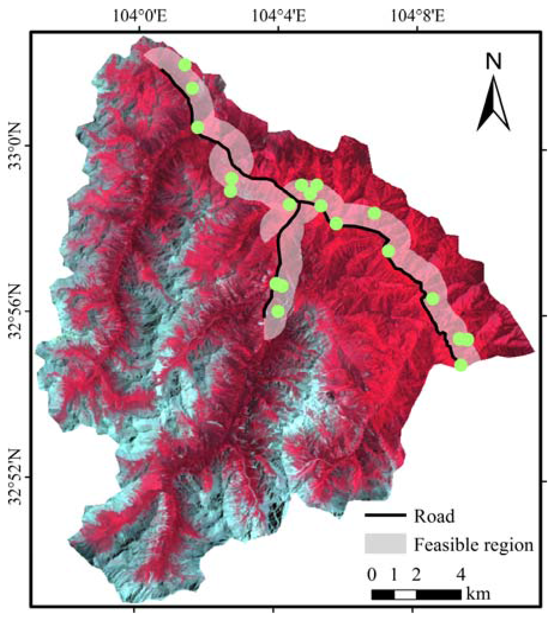
Figure 4.
NDVI frequency distribution histograms of 20 selected elementary sampling units for the four sampling strategies (from top to bottom): random sampling (RS), single-temporally constrained sampling (SC), and multi-temporally constrained sampling (MC) in the feasible region (MC) and in the entire study area without the sampling feasible constraint (MCE). The red lines represent the NDVI frequency distribution histograms of the entire study area.
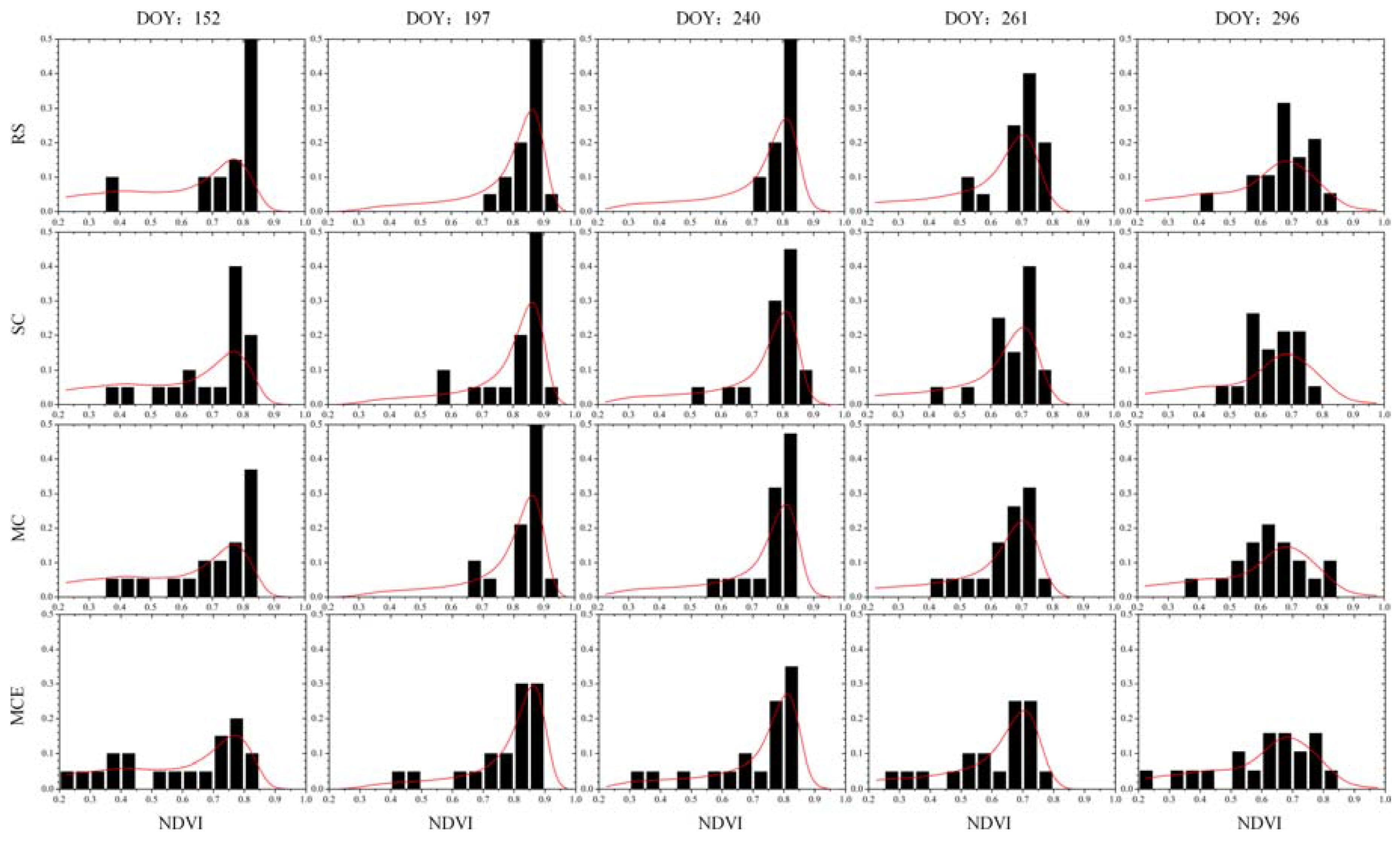
Figure 5.
Scatterplots between the average sampled NDVI and the average true NDVI values for the entire study area and for the five different dates. (a) Random sampling in the feasible region. (b) Single-temporally constrained sampling in the feasible region. (c) Multi-temporally constrained sampling in the feasible region. (d) Multi-temporally constrained sampling in the entire region. The bars indicate the standard deviations.

Figure 6.
Density scatterplots between the NDVI and the cosine of the local solar incidence angle (cos(i)) in Wanglang study area for the different acquisition dates.
Figure 6.
Density scatterplots between the NDVI and the cosine of the local solar incidence angle (cos(i)) in Wanglang study area for the different acquisition dates.


Table 1.
Overview of Landsat data (path: 130, row: 37) used in this study.
| DOY | Year | Satellite/Sensor |
|---|---|---|
| 152 | 2014 | Landsat 8/OLI |
| 197 | 2013 | Landsat 8/OLI |
| 240 | 2011 | Landsat 5/TM |
| 261 | 2007 | Landsat 5/TM |
| 296 | 2014 | Landsat 8/OLI |
Table 2.
Overlapping area (OA, %) for random sampling (RS), single-temporally constrained sampling (SC), and multi-temporally constrained sampling applied to the feasible region (MC) and to the entire study area (MCE).
Table 2.
Overlapping area (OA, %) for random sampling (RS), single-temporally constrained sampling (SC), and multi-temporally constrained sampling applied to the feasible region (MC) and to the entire study area (MCE).
| DOY | RS | SC | MC | MCE |
|---|---|---|---|---|
| 152 | 50.3 | 64.2 | 72.2 | 85.8 |
| 197 | 72.0 | 75.9 | 71.3 | 82.3 |
| 240 | 62.2 | 70.7 | 74.1 | 83.2 |
| 261 | 63.2 | 67.8 | 82.9 | 84.0 |
| 296 | 68.0 | 65.0 | 72.8 | 82.0 |
| Annual mean | 63.1 | 68.7 | 74.7 | 83.5 |
© 2017 by the authors. Licensee MDPI, Basel, Switzerland. This article is an open access article distributed under the terms and conditions of the Creative Commons Attribution (CC BY) license (http://creativecommons.org/licenses/by/4.0/).
Share and Cite
MDPI and ACS Style
Yin, G.; Li, A.; Verger, A. Spatiotemporally Representative and Cost-Efficient Sampling Design for Validation Activities in Wanglang Experimental Site. Remote Sens. 2017, 9, 1217. https://doi.org/10.3390/rs9121217
AMA Style
Yin G, Li A, Verger A. Spatiotemporally Representative and Cost-Efficient Sampling Design for Validation Activities in Wanglang Experimental Site. Remote Sensing. 2017; 9(12):1217. https://doi.org/10.3390/rs9121217
Chicago/Turabian StyleYin, Gaofei, Ainong Li, and Aleixandre Verger. 2017. "Spatiotemporally Representative and Cost-Efficient Sampling Design for Validation Activities in Wanglang Experimental Site" Remote Sensing 9, no. 12: 1217. https://doi.org/10.3390/rs9121217
Note that from the first issue of 2016, this journal uses article numbers instead of page numbers. See further details here.