Rolling Guidance Based Scale-Aware Spatial Sparse Unmixing for Hyperspectral Remote Sensing Imagery


1
School of Computer Science, China University of Geosciences (Wuhan), Wuhan 430074, China
2
State Key Laboratory of Information Engineering in Surveying, Mapping, and Remote Sensing, Wuhan University, Wuhan 430079, China
3
School of Resource and Environmental Sciences, Wuhan University, Wuhan 430079, China
*
Authors to whom correspondence should be addressed.
Remote Sens. 2017, 9(12), 1218; https://doi.org/10.3390/rs9121218
Submission received: 9 October 2017
/
Revised: 18 November 2017
/
Accepted: 23 November 2017
/
Published: 26 November 2017
(This article belongs to the Section Remote Sensing Image Processing)
Abstract
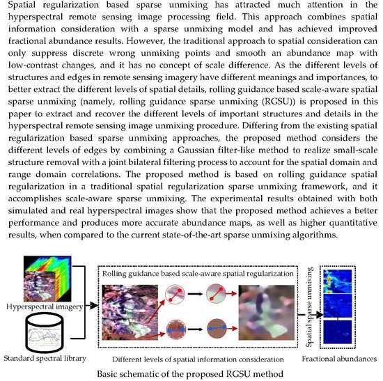
:Spatial regularization based sparse unmixing has attracted much attention in the hyperspectral remote sensing image processing field, which combines spatial information consideration with a sparse unmixing model, and has achieved improved fractional abundance results. However, the traditional spatial sparse unmixing approaches can suppress discrete wrong unmixing points and smooth an abundance map with low-contrast changes, and it has no concept of scale difference. In this paper, to better extract the different levels of spatial details, rolling guidance based scale-aware spatial sparse unmixing (namely, Rolling Guidance Sparse Unmixing (RGSU)) is proposed to extract and recover the different levels of important structures and details in the hyperspectral remote sensing image unmixing procedure, as the different levels of structures and edges in remote sensing imagery have different meanings and importance. Differing from the existing spatial regularization based sparse unmixing approaches, the proposed method considers the different levels of edges by combining a Gaussian filter-like method to realize small-scale structure removal with a joint bilateral filtering process to account for the spatial domain and range domain correlations. The proposed method is based on rolling guidance spatial regularization in a traditional spatial regularization sparse unmixing framework, and it accomplishes scale-aware sparse unmixing. The experimental results obtained with both simulated and real hyperspectral images show that the proposed method achieves visual effects better and produces higher quantitative results (i.e., higher SRE values) when compared to the current state-of-the-art sparse unmixing algorithms, which illustrates the effectiveness of the rolling guidance based scale aware method. In the future work, adaptive scale-aware spatial sparse unmixing framework will be studied and developed to enhance the current idea.
1. Introduction
In the last decade, airborne and satellite hyperspectral remote sensing sensors have developed at an enormous rate, resulting in the availability of a large volume of hyperspectral remote sensing data with a wealth of spectral information and a higher spectral resolution, which covers a wider wavelength region with hundreds of spectral channels at a nominal spectral resolution. The resulting hyperspectral date cube enables precise material identification with the abundance spectral information, as each pixel can be represented by a spectral signature or fingerprint that characterizes the underling objects [1,2]. However, one of the challenges confronting hyperspectral remote sensing image processing is the presence of mixed pixels [3,4,5]. Spectral unmixing is a common way to solve this mixed pixel problem, and it is aimed at estimating the fractional abundances of the pure spectral signatures or endmembers in each mixed pixel with linear or nonlinear mixture models [6,7]. The linear mixture model expresses the measured spectral signature as a linear combination of several distinct typical materials or endmembers, while the nonlinear mixture model assumes that the incident radiation interacts with more than material, and it is affected by multiple scattering effects [8]. When compared with the nonlinear mixture model, the linear mixture model has been extensively studied as a result of its computational tractability and its flexibility in different applications, and the fact that it also holds in macroscopic remote sensing scenarios. Therefore, in this paper, we focus on linear spectral unmixing analysis.
The traditional spectral unmixing approaches consist of three basic ideas to precisely estimate the endmember signatures and the corresponding fractional abundances. One idea can be called the supervised methods, which compute the abundances or endmember signatures based on the known precise endmember signatures [9,10] or abundances [11,12]. The second idea is the unsupervised methods, which are sometimes referred to as Blind Source Separation (BSS) [13,14,15,16,17], which assume that the spectral components are statistically independent. The last idea is the semi-supervised methods, which express the mixed pixels using a large standard spectral library known in advance, and estimate the fractional abundances, as well as activating the corresponding materials’ standard spectral signatures [18,19,20,21]. Approaches of the first series have been studied for many years, and include the Pixel Purity Index (PPI) [22], N-FINDR [23], Fully Constrained Least Squares (FCLS) [9], and Abundance-Constrained Endmember Extraction (ACEE) [11]. Independent Component Analysis (ICA) [24], Non-negative Matrix Factorization (NMF) [25], and Sparse Component Analysis (SCA) [26] belong to the second spectral unmixing idea. In recent years, the semi-supervised unmixing methods have attracted lots of attention as they make full use of a standard spectral library, and they also effectively circumvent the challenging endmember identification step [2], which is replaced with activating the corresponding endmember signatures over the large standard spectral library, which is given as prior knowledge.
Sparse unmixing, as one of the typical semi-supervised spectral unmixing methods, reformulates the linear spectral unmixing problem as selecting endmembers from a standard spectral library using sparse regression [8]. Since the research into sparse unmixing has progressed, a number of sparse unmixing algorithms have been proposed, such as Sparse Unmixing via variable Splitting and Augmented Lagrangian (SUnSAL) [27], Sparse Unmixing via variable Splitting and Augmented Lagrangian and Total Variation (SUnSAL-TV) [28], Non-Local Sparse Unmixing (NLSU) [29], and Collaborative SUnSAL (CSUnSAL) [19], and its variants [30,31]. Spatial sparse unmixing incorporates the spatial information into sparse unmixing and utilizes the existing spatial correlations, leading to a higher unmixing accuracy and a better visual effect [32]. Hence, the spatial sparse unmixing methods should be a worthwhile approach for hyperspectral remote sensing image processing.
The current spatial-spectral unmixing methods usually use the spatial information between each pixel and its near neighbors, e.g., the Total Variation (TV)-based regularization model [33] and the mathematical morphological methods [34], or region-based spatial consideration, e.g., the sliding-window based approaches [35]. Most of these approaches aim to preserve the edges and remove detrimental or unwanted content. However, with the spatial regularization based methods, only high-contrast edges or textures can be extracted, and low-contrast or gradual changes in the original remote sensing images are ignored, which results in the loss of small structures, which are usually referred to as “details”.
In this paper, a new spatial sparse unmixing algorithm based on rolling guidance as a scale-aware operation, namely, Rolling Guidance Sparse Unmixing (RGSU), is proposed. In RGSU, the rolling guidance scale-aware model [36] is designed as the spatial regularization by considering and controlling the different level of details with iterations following scale-space theory. The rolling guidance idea has been used in image denoising, detail enhancement, edge extraction, image segmentation, saliency detection, and so on [37,38,39]. Differing from the previous spatial sparse unmixing methods, the proposed RGSU algorithm is scale-aware and can separate the different detail levels and achieve unmixing results with clear boundaries or texture information and clear background regions. When compared with the previous spatial sparse unmixing algorithms, the experimental results obtained using two simulated hyperspectral datasets and two real hyperspectral images demonstrate that the proposed RGSU can obtain improved fractional abundances images and a higher unmixing accuracy.
The rest of this paper is organized as follows. In Section 2, the spatial sparse unmixing model (the rolling guidance spatial regularization model) and the proposed RGSU algorithm are presented. Section 3 provides a description of the datasets that are used in this paper and analyzes the experimental results. The conclusion is drawn is Section 4.
2. Rolling Guidance Based Spatial Sparse Unmixing
Spatial regularization based sparse unmixing can integrate spatial information into the sparse unmixing process and obtain improved spectral unmixing results. Differing from the previous spatial sparse unmixing methods, such as SUnSAL-TV or NLSU, the rolling guidance based spatial regularization method can recognize objects of different sizes and preserve structures of various scales, which delivers diverse information. Hence, in theory, the results of the rolling guidance based spatial sparse unmixing algorithm better preserve spatial information.
In this part, the traditional spatial sparse unmixing model is first reviewed in Section 2.1, and then the rolling guidance spatial regularization model is described in detail in Section 2.2. Finally, based on the aforementioned model and prior knowledge, the proposed rolling guidance based scale-aware spatial sparse unmixing algorithm, the RGSU algorithm, is described in Section 2.3.
2.1. Spatial Sparse Unmixing
To improve the unmixing accuracy and treat the hyperspectral remote sensing datasets as images, spatial information can be incorporated into the sparse unmixing formulation by adding an appropriate spatial regularization, and the spatial sparse unmixing model has thus been developed. Since the traditional sparse unmixing problem can be written, as shown in Equation (1), which considers the Abundance Non-negative Constraint (ANC), the spatial sparse unmixing model can be specified as a minimization function and is rewritten, as shown in Equation (2), based on the classical sparse unmixing model:
where y = (y1, y2, …, yL)T is a mixed pixel, and L is the number of spectral bands. denotes the large available spectral library, and m is the number of endmembers in A. In Equation (1), x = (x1, x2, …, xm)T represents the fractional abundance vector corresponding to spectral library A. Due to the fact that only a small number of endmembers, e.g., less than 20 [8], contribute to a mixed pixel y, x is sparse. denotes the sparse constraint of the fractional abundance vector x, which is a relaxation of the original L0 norm [29]. is the error tolerance derived from the noise or modeling errors. denotes the ANC.
In Equation (2), denotes the observed hyperspectral dataset containing n pixels with L bands, written in the form of a matrix. is the fractional abundance map, corresponding to the input hyperspectral dataset Y. is the data-fitting term, and denotes the Frobenius norm. , and denotes the j-th column of X [40]. The last term, , is aimed at finding the minimum element of the abundance vector xj, and it also denotes the ANC. The function in Equation (2) is defined in the set C, obeying the rule of when ; otherwise, .
When compared with Equation (1), there is an extra term in Equation (2), the consideration of spatial information, written as Jspt(X), which is used for incorporating the spatial information. Different consideration of the spatial information leads to different spatial smoothness terms Jspt(X) [33]. For example, the TV-based sparse unmixing algorithm utilizes the TV model as the spatial regularization to account for spatial homogeneity. Nonlocal TV-based sparse unmixing also accounts for all of the possible nonlocal spatial information in the sparse unmixing process. In general, the spatial sparse unmixing model can be expressed, as shown in Equation (2), when only the ANC is considered.
2.2. Rolling Guidance Spatial Regularization Model
As remote sensing images contain many levels of structures, edges, and details, the important small structures should be preserved and the anomaly objects or noise should be removed in the hyperspectral image processing [41,42], which is also the original motivation of the spatial sparse unmixing methods. TV-based regularization in the sparse unmixing model accounts for the neighboring mixed pixels of the fractional abundance map with the same endmember combination. It can better preserve and restore high-contrast edges between the current pixel and its horizontal and vertical neighbors [33]. The nonlocal sparse unmixing method uses a nonlocal means regularizer to utilize all of the possible self-predictions of the similar sparse distributions in the abundance images [35], and the range for the spatial information extraction depends on a sliding window of a fixed size. Both of these spatial consideration approaches protect most of the structural edges in the abundance maps. However, these methods basically preserve the conspicuous changes and efficiently remove low-level spatial stochastic noise, but they cannot separate the different levels of details and structures [43].
Rolling guidance spatial regularization is a structure-scale-aware operation that is aimed at controlling and preserving the different levels of details under different image processing demands. In this paper, the structure scale [44] is defined as the smallest Gaussian standard deviation, and the corresponding structure of this scale can be removed or smoothed when this deviation is applied to an image. Generally, through the whole rolling guidance spatial consideration process, only one Gaussian standard deviation will be chosen. To some extent, the scale-aware rolling guidance spatial regularization plays the role of a Gaussian filter at the initial step, where the initialized convolution kernel is related to the structure scale, namely, the scale parameter in scale-space theory, which is written as shown in Equation (3):
where v is referred to as the scale parameter whose value is equal to the variance of the abundance image. denotes the Gaussian kernel, which indexes pixels i and j, and represents the convolution operation. X is the input abundance image, and Gv represents the initial result at scale v in the first step of the scale-aware rolling guidance process. When different Gaussian standard deviations () are applied as the image spatial regularization, different scales of structures can be suppressed according to their actual sizes.
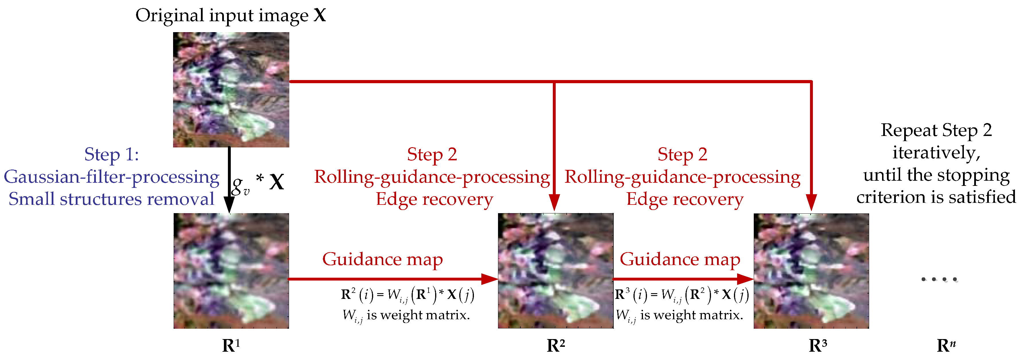
In the second step, the edges that are processed by the Gaussian filter are retained according to their input guidance map. Here, the rolling guidance process provides the scale-aware spatial regularization, which is aimed at recovering the important edges iteratively, and the input guidance map forms the major contribution of this scale-aware method. We denote Rt as the t-th iteration guidance map, and R1 is initialized as Gv. The output of this second step, which is written as Rt+1 for the t-th iteration rolling guidance result, can be obtained as follows:
with
where i and j represent the i-th and j-th pixels, N(i) denotes a local window of size around pixel i, is the weight for the rolling guidance method, and is a normalization term, which is computed, as shown in Equation (6). The value of Rt+1 is obtained in the form of joint bilateral filtering [45,46], considering the distance in the image plane (the two-dimensional (2-D) spatial domain of the abundance map) and the distance in the intensity axis (the range domain). In addition, v is the scale parameter, and r defines the weight of the intensity decrease degree. The weight of the rolling guidance filter is computed in the form of a joint bilateral filter guided by the structure of Rt, which is iteratively changed in the processing. This is the reason why this scale-aware iterative operation is named “rolling guidance”, and it is also the key difference with the classical joint bilateral filter. The flowchart of the scale-aware rolling guidance method is provided in Figure 1.
2.3. Rolling Guidance Based Spatial Sparse Unmixing
To better address the different scales of spatial information in sparse unmixing, the Rolling Guidance based Sparse Unmixing method (RGSU) is proposed for the scale-aware spatial consideration of hyperspectral remote sensing unmixing. Based on rolling guidance spatial regularization and the spatial sparse unmixing model, the rolling guidance based spatial sparse unmixing method is built up as follows:
where the first term is denoted as the data-fitting term, and the second one, the L1,1 norm of the abundance, is used for sparse constraint, which corresponds to the fact that the observed hyperspectral image signature can be expressed in an efficient linear sparse regression with potentially very large endmember dictionary [8], denoted as A. The last term is represented by the ANC. In addition, the third term, rolling guidance spatial regularization, can be written as:
where the weight matrix is defined for different spatial considerations, and is obtained following the original rolling guidance method, as Equation (9):
with
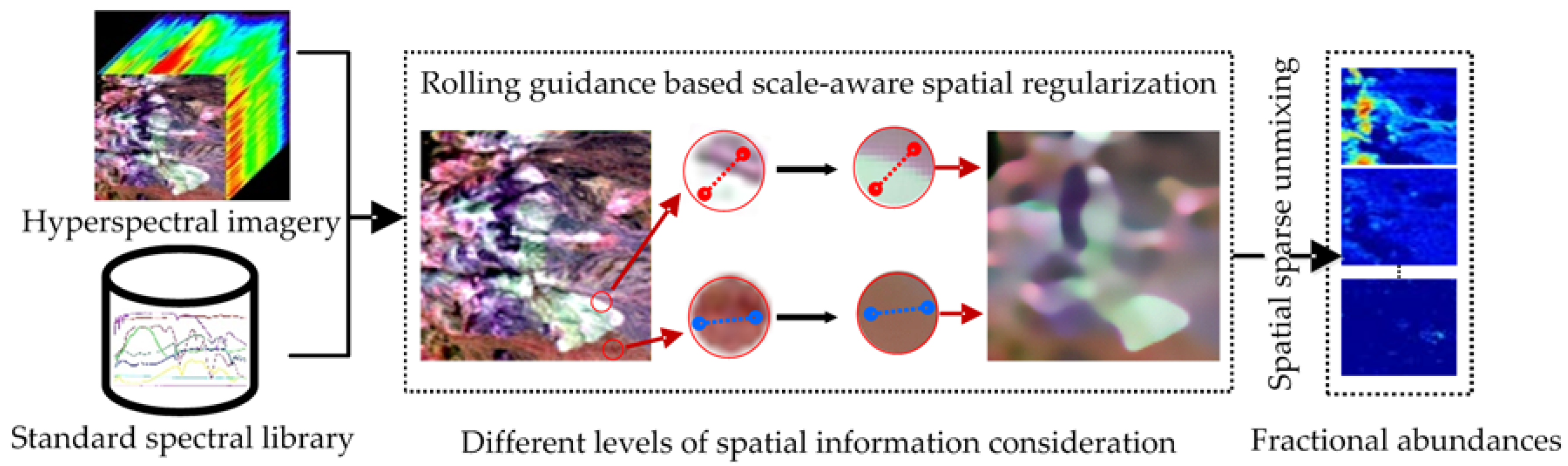
In this scale-aware spatial regularization sparse unmixing procedure, the weight matrix [47,48] accounts for filtering and averaging the differences in a local window, such as outliers and noise, which can remove structures in different scales. The input abundance map, X, is the guidance map, which is used to recover shapes of different scales. Whether an edge is preserved or not is dependent solely on its magnitude, making this method inherently different to the other edge-preserving methods. By setting different scale values, this scale-aware spatial sparse unmixing algorithm can contain different-scale levels of spatial information. The basic schematic of the proposed method can be depicted, as shown in Figure 2.
Based on the above constructed objective function, the main process of how to compute the RGSU model is introduced below.
Given the objective function (Equation (7)) and following the classical split Augmented Lagrangian method of Multipliers (ALM) for solving the sparse representation problem, a few intermediate variables are introduced in Equation (7) for convenient representation. We first develop the augmented objective function, as shown as Equation (11). In addition, the Alternating Direction Method of Multipliers (ADMM) strategy is also adopted.
with
where and the other terms multiplied by the multiplier (μ > 0) are the augmented terms related to the terms of the main function, such as . are also parts of the ADMM strategy satisfying: .
The main steps for solving the RGSU problem are listed in Algorithm 1.
| Algorithm 1 |
|
3. Experiments and Analysis
To evaluate the performance of the proposed method, two simulated hyperspectral datasets and two real hyperspectral images were used to illustrate the different unmixing performances. The proposed method was compared with three state-of-the-art sparse unmixing algorithms: Sparse Unmixing via variable Splitting and Augmented Lagrangian (SUnSAL), Sparse Unmixing method based on Noise Level Estimation (SU-NLE) [49], Sparse Unmixing via variable Splitting and Augmented Lagrangian and Total Variation (SUnSAL-TV), and Non-Local Sparse Unmixing (NLSU). The accuracy assessment of all the experiments in this paper was made by the Signal-to-Reconstruction Error (SRE) [50], which is defined as follows:
3.1. Experimental Datasets
The first simulated dataset was generated following the methodology described in [50], with 75 × 75 pixels and 224 bands per pixel, using randomly selected spectral signatures from library A, which is denoted as splib06 (http://speclab.cr.usgs.gov/spectral.lib06). In addition, the abundance sum-to-one constraint and ANC were both imposed in the simulation process. Finally, i.i.d. Gaussian noise was added with a Signal-to-Noise Ratio (SNR) of 30 dB. In the final simulated hyperspectral image, there were pure regions as well as mixed regions that were constructed using two to five endmembers, distributed in different distinct square regions. The background pixels were also highly mixed, with five endmembers. Figure 3 shows the selected spectral signatures of this dataset, as well as the true abundance maps corresponding to the five endmembers.
Simulated dataset 2, with 100 × 100 pixels and 224 bands, was provided by Dr. M. D. Iordache and Prof. J. M. Bioucas-Dias. The fractional abundances of this dataset follow a Dirichlet distribution uniformly over the probability simplex. Since this image exhibits a good spatial homogeneity and can be used to verify the different effects of the spatial regularization spectral unmixing methods, this dataset has been widely used to test many spatial sparse unmixing algorithms. Figure 4 displays the nine spectral signatures that were used to simulate this dataset and the true abundance images. Gaussian noise of 30 dB was also added in the data simulation process.
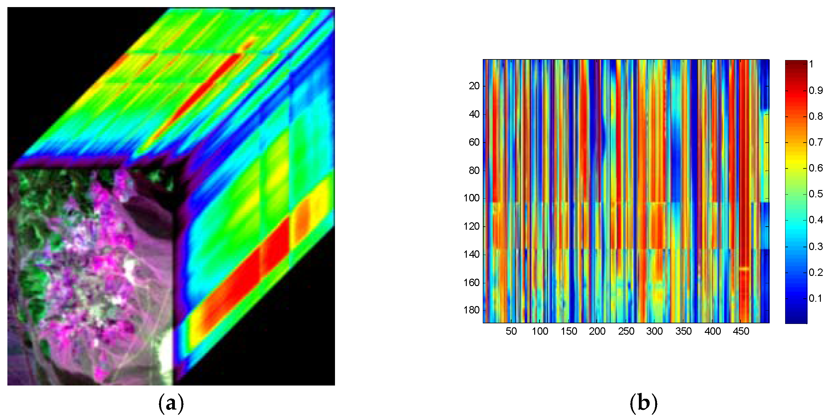
The first real hyperspectral remote sensing image we chose was the Cuprite dataset, which has been widely used in hyperspectral unmixing analysis. This image was collected in 1997 from the Cuprite mining district in west-central Nevada by the Airborne Visible InfraRed Imaging Spectrometer (AVIRIS), and comprises 224 bands ranging from 0.4 to 2.5 μm. The spatial resolution of this image is 20 m per pixel, which leads to the mixture of different minerals. In our experiment, the test area was of 250 × 191 pixels, with 188 bands remaining after removing the bands of strong water absorption and low SNR vales. The standard spectral library used for all of the sparse unmixing algorithms was the United States Geological Survey (USGS) spectral library, which contains 498 pure mineral signatures. After essential calibration was undertaken, the final dataset that was used in our experiment is shown in Figure 5.
The second real hyperspectral image (Nuance data) [51], with 50 × 50 pixels and 46 bands, was obtained by a Nuance NIR imaging spectrometer, whose spectral wavelength ranges from 650 nm to 1100 nm, with a spectral resolution of about 10 nm. This dataset was collected in our outdoor experiment, and the corresponding land-cover material signatures, which contain 52 materials, were also observed and collected during the same time period. In order to undertake a quantitative assessment, a higher spatial resolution multi-spectral image, denoted as HR (Higher-Resolution RGB image), was also captured on the same day using a digital camera. The HR data image was of 150 × 150 pixels, with red, green, and blue bands. In our experiment, the geometrical calibration, classification, and down-sampling were undertaken on the HR image in advance so as to obtain the approximate reference abundance maps. The original hyperspectral image data, the spectral library for this dataset, the HR data, and the approximate reference abundance map are shown in Figure 6.
The basic information about the above four datasets can be concluded in Table 1, as follows, which includes the type of sensors, image size and the corresponding number of bands, as well as the Signal-to-Noise Ratio (SNR) values.
3.2 Results and Analysis
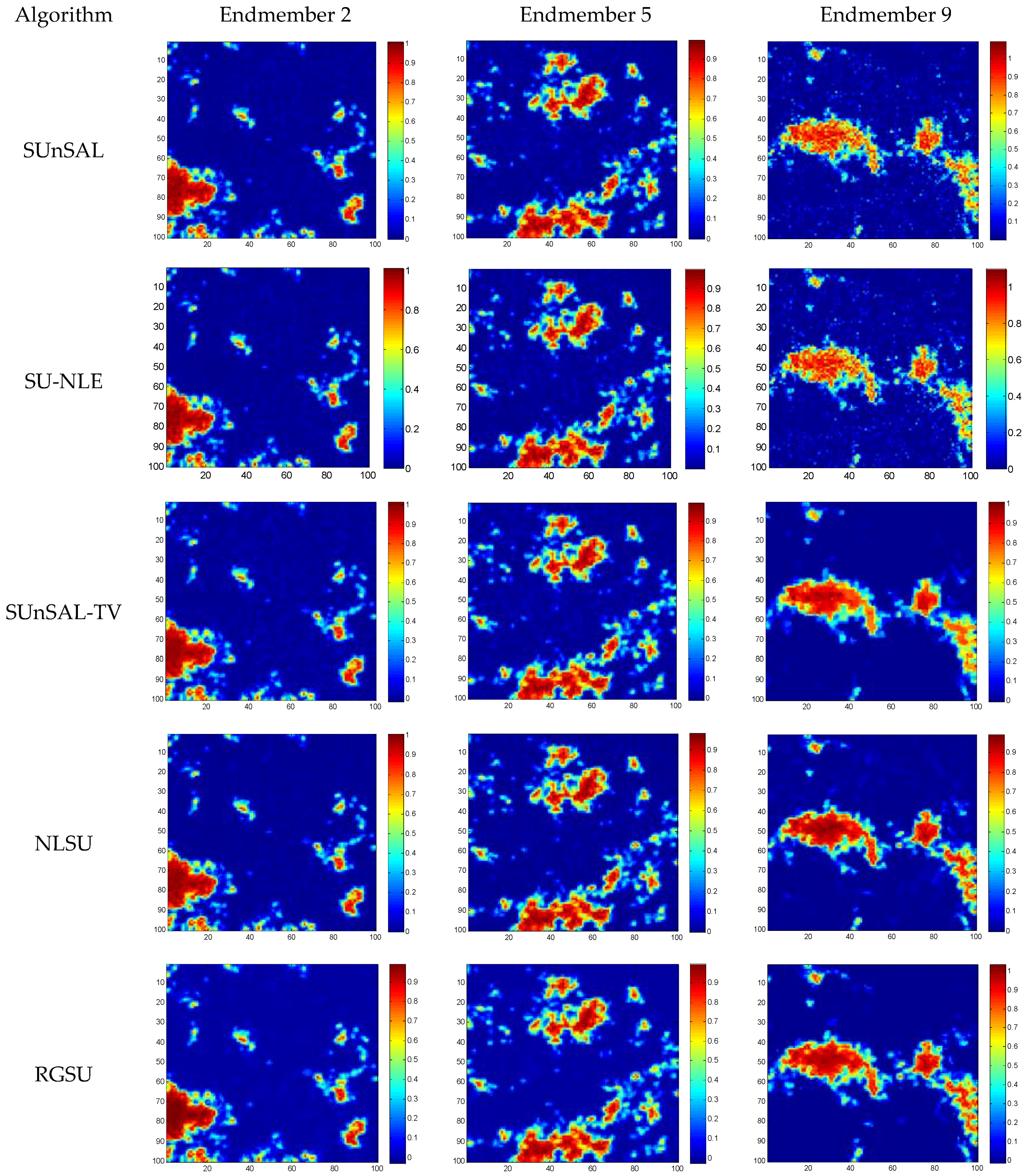
The results obtained using SUnSAL, SU-NLE, SUnSAL-TV, NLSU, and the proposed RGSU with the two simulated datasets and the two real hyperspectral images are shown in Figure 7, Figure 8, Figure 9 and Figure 10, respectively. Qualitative and quantitative assessments were made from both visual comparisons and SRE values. The quantitative results, as well as the parameters, are listed in Table 2.
The different estimated abundances obtained by different sparse unmixing algorithms for simulated dataset 1 are shown in Figure 7. It can be observed that the spatial regularization based sparse unmixing obtains significantly better results than the classical sparse unmixing method, SUnSAL and SU-NLE. Spatial regularization based sparse unmixing approaches can strongly suppress the wrong unmixing abundances, which illustrates the effectiveness of the spatial consideration. When compared with SUnSAL-TV and NLSU, RGSU displays more a homogeneous background and foreground (the small squares), which is the direct result of rolling guidance method, controlling and preserving the structure-scales of the original hyperspectral image. Moreover, RGSU outperforms the other methods, especially in preserving the edges of the details and suppressing the outliers in small-scale noise. For example, as compared with SUnSAL-TV and NLSU, the square edges of the fractional abundance map of endmember 2 obtained by RGSU are more clearly defined. In addition, as the background of the abundance map for one specific endmember has a fixed fractional abundance value, the ideal unmixing result for the background should be one solid color. After spatial consideration and the denoising-type unmixing processing, the fractional abundances that are obtained by RGSU show the best results in Figure 7.
Figure 8 shows a visual comparison of the estimated abundance maps for simulated dataset 2. Since this dataset exhibits a good spatial homogeneity, the different spatial regularization based sparse unmixing methods show different processing effects. Due to the lack of spatial consideration, the abundance maps that are obtained by SUnSAL and SU-NLE have many outliers left, which are distributed as discrete noise points. In our simulated datasets experimental settings, since the noise levels added to the simulated dataset are simple and the intensities of different bands are same, the advantage of SU-NLE algorithm has not been revealed, as SU-NLE can better alleviate the impact of different noise levels at different band during the sparse unmixing process and enhance the unmixing performance. SUnSAL-TV, NLSU, and RGSU effectively suppress the outliers owning to the adequate spatial consideration. However, among the different spatial regularization based sparse unmixing approaches, RGSU obtains better unmixing results, both in suppressing the wrong unmixing points of the background and in processing the edge changes. It can be seen that RGSU successfully handles the different scales of structures and edges in the images.
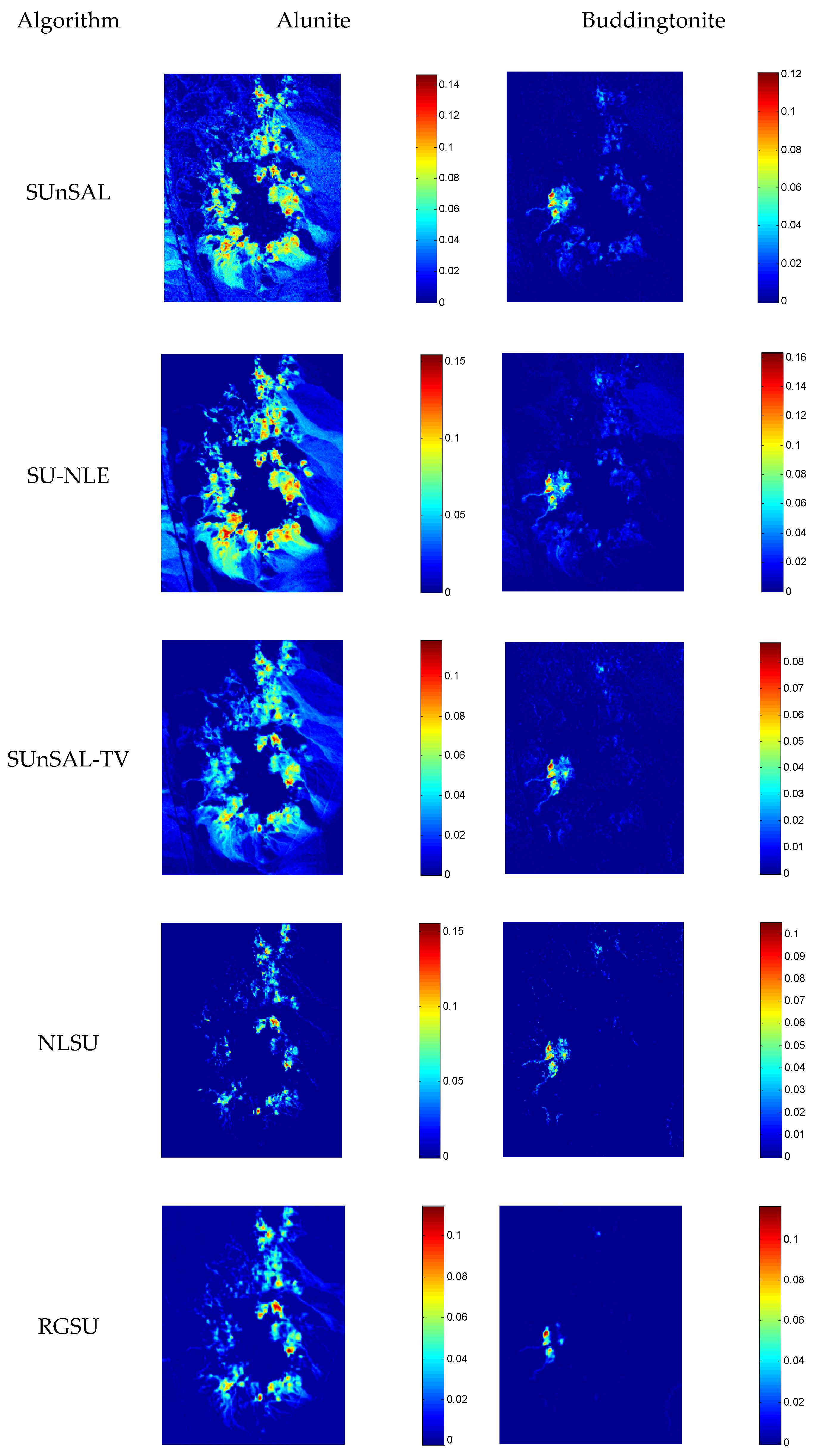
Similarly, a qualitative comparison for cuprite data between the abundance images was made with SUnSAL, SU-NLE, SUnSAL-TV, NLSU, and RGSU for alunite and buddingtonite. Different from the simulated datasets and the following Nuance data, due to the lack of ground truth for the Cuprite dataset, Figure 9 just shows a visual comparison of the estimated abundance maps for this data. The fractional abundance images obtained by RGSU are generally consistent with the abundance of images that are obtained by the other different methods, but there are some differences in the details. For example, the homogeneity of the RGSU result is more obvious, which can be observed in the buddingtonite component, as the minerals locating in the background are suppressed due to the small scale. The abundance map of alunite appears to be similar to the result of SUnSAL-TV, which preserves more information than the abundance that is obtained by NLSU. After comprehensive analysis and judgment, this can be attributed to the rolling guidance spatial regularization in sparse unmixing.
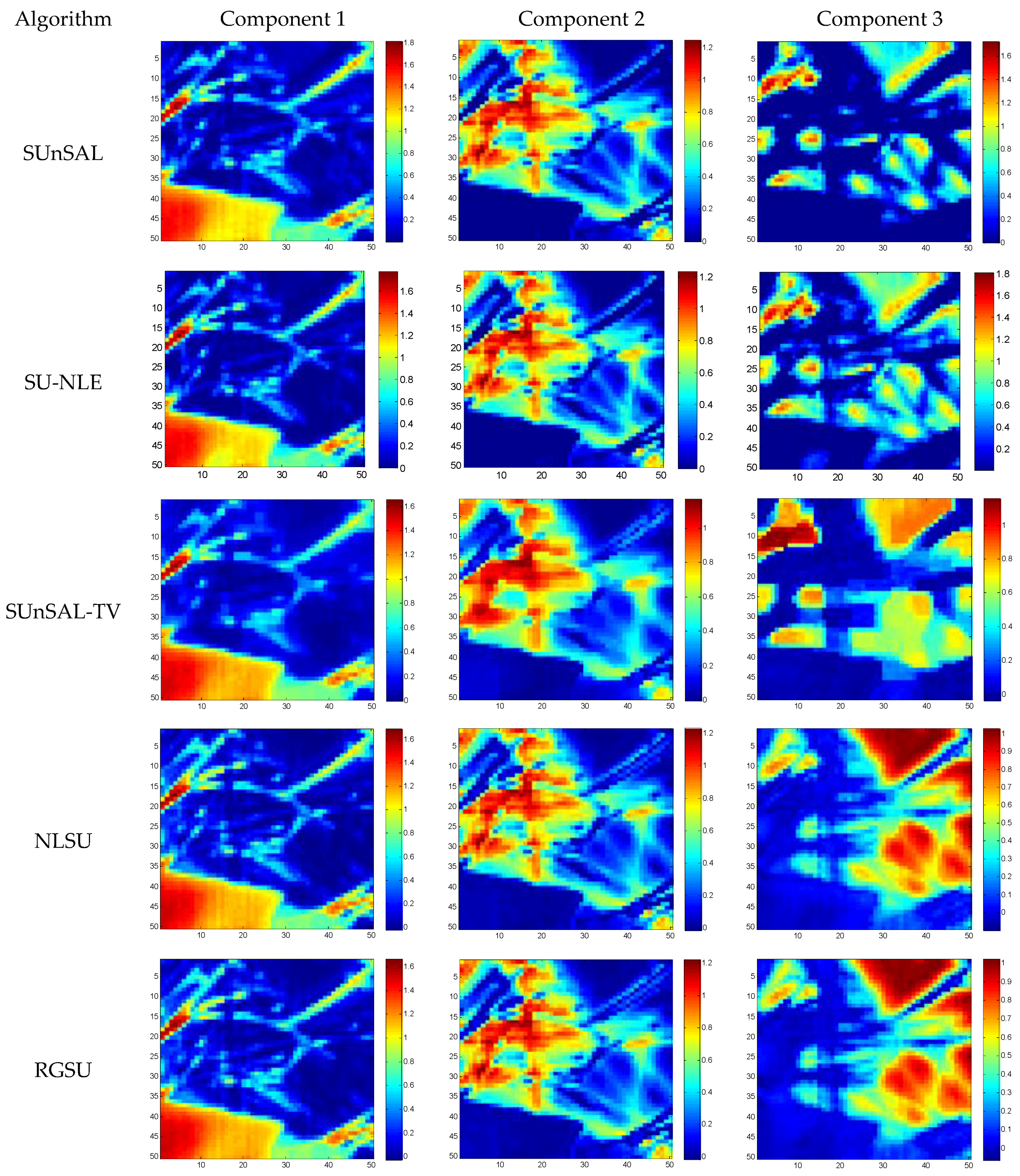
From Figure 10, it can be observed that the fractional abundance maps that are obtained by NLSU and the proposed RGSU are quite similar, especially in the homogeneous regions, such as the area of the leaves in component 1 or the background in component 3. However, since RGSU deals with spatial information in different ways, it exploits different structures, as well as different scales differently. For example, in the background of component 3, there are some details of the thin leaves with low fractional abundance values in the NLSU result, while these small differences are wiped off and the significant edges are clearly preserved in the result of RGSU. When compared with RGSU and NLSU, the abundances of SUnSAL, SU-NLE, and SUnSAL-TV both reveal obvious defects and limitations. Hence, the scale-aware rolling guidance based sparse unmixing algorithm shows some advantages over the traditional spatial regularization based sparse unmixing approaches.
Table 2 displays a quantitative comparison of SUnSAL, SU-NLE, SUnSAL-TV, NLSU, and RGSU for the above three datasets, i.e., simulated dataset 1, simulated dataset 2, and the Nuance data. Since there is no reference abundance map or ground truth for Cuprite dataset, Nuance data is set as an example for real hyperspectral dataset and the fractional abundances that are obtained by Cuprite data are just for qualitative comparison between the abundance images by applying different sparse unmixing methods. When compared with the classical sparse unmixing method, the spatial regularization based sparse unmixing methods obtain a much better unmixing accuracy with significantly higher SRE values. For example, for simulated dataset 1, the SRE values of the SUnSAL and SU-NLE algorithm are around 15 dB, while the SRE values increases to 30 dB after taking spatial information into consideration. Meanwhile, the different spatial regularization approaches lead to different spatial consideration and different spatial sparse unmixing effects. The TV-based spatial regularization sparse unmixing methods are better able to extract the spatial homogeneity of the first-order pixel neighborhood system, and the nonlocal TV-based spatial sparse unmixing algorithm accounts for all of the possible self-predictions of the similar sparse distributions. These two methods both incorporate spatial information of the abundance images into the sparse unmixing process, but the different methods both have their limitations. The proposed rolling guidance based sparse unmixing algorithm reconsiders the spatial information in the form of scale, and the quantitative results demonstrate the advantages over the TV-based and nonlocal TV-based sparse unmixing methods, especially in the datasets with significant scale differences. In the quantitative comparison, the proposed method has obtained higher SRE values and the highest increase is about 3.6677 dB when compared with the NLSU algorithm. The visual effects are also constant with the quantitative results.
The running times of the different algorithms for these three datasets are also provided in Table 2 with an Intel Core i7-6700 CPU @3.4 GHz and 16 GB RAM, using MATLAB R2014a. Since the different coding strategies would lead to different running times, Table 2 just gives us a relative time consumption. From this table, it can be observed that the proposed algorithm, RGSU, needs more time to compute structure-scale values. In future work, more study should be made to enhance the computational efficiency of the proposed method.
3.3. Sensitivity Analysis
3.3.1. Discussion on Sensitivity Analysis for the Inner Parameters, v and r
In the proposed method, there are two important inner parameters in the rolling guidance scale-aware spatial regularization term, v and r, where v is denoted as the scale parameter and r is used to define the weight of the intensity decrease degree. Different values of the scale parameter affect the spatial extraction performance and the different weights of intensity decrease degree lead to different spatial processing results. To better understand the effect of these two parameters, we analyzed the selection of v and r with simulated dataset 1. The SRE (dB) values obtained with the different combinations of v and r for RGSU are shown in Figure 11, with multiple color-map surfaces. The three-dimensional (3D) color-map surfaces represent the different results of the different combinations of v and r in this algorithm.
The relationship between the SREs and these two inner parameters is shown in Figure 11. This figure gives us empirical ranges for these two important inner parameters, i.e., parameter v should be set around 3 and parameter r should be set around 0.01. In our experiments, parameters v and r were set around 3 and 0.01, respectively, which controls the extraction scales of spatial details and the intensity decrease degree in spatial scale recovery process. In our future research, an adaptive method of parameter selection will be studied and developed to enhance the scale-aware spatial regularization based sparse unmixing method.
3.3.2. Discussion on Sensitivity Analysis for the Regularization Parameters, λsps and λRG
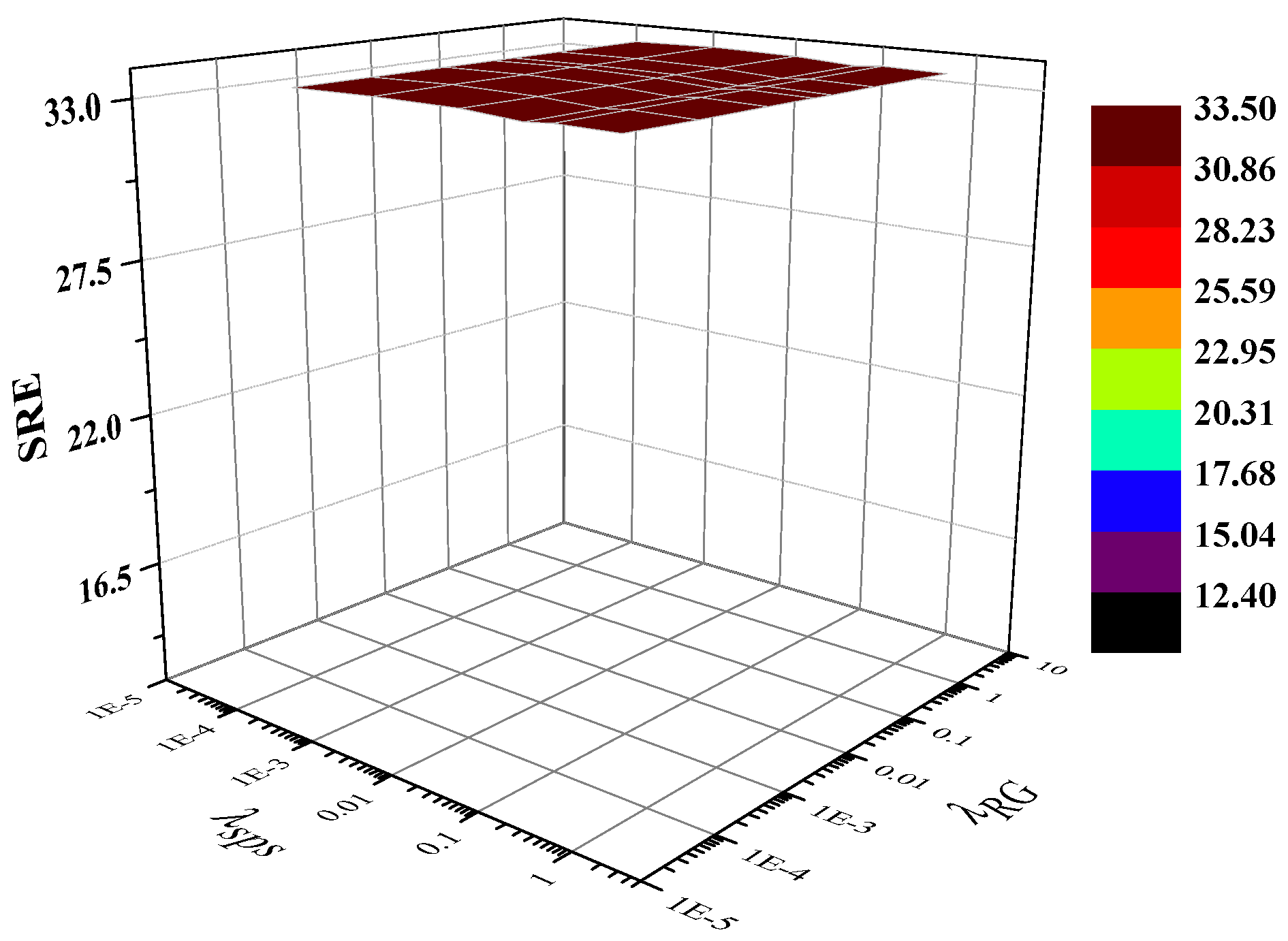
In spatial regularization based sparse unmixing approaches, there are always two regularization parameters, λsps and λRG, which play important roles in the objective functions. As they can tradeoff the weights of the different terms, it is a necessary step to properly set these two values. Figure 12 analyzes the impact of these two parameters with a series of different combination of λsps and λRG in the RGSU algorithm for the simulated dataset 1 as an example.
As shown in Figure 12, it can be observed that the best combination of parameters, λsps and λRG in RGSU with simulated dataset 1 can be chosen in a wide range for simulated dataset 1, and most of them lead to relatively optimal SRE dB values of about 33.30 dB. However, improper combination of these two regularization might also fail to obtain normal solution, 12.40 dB or 15.04 dB, for example. Because of the small number and the locations of the abnormal values, it is not quite obvious in Figure 12. Since different datasets may have different characters in real circumstances, to achieve a relatively better quantitative results, or higher SRE dB values, and to exploit the more precisely scale spatial information, appropriate regularization parameters’ combination should be chosen according to the quality of hyperspectral imagery, as well as the spatial information in the scene.
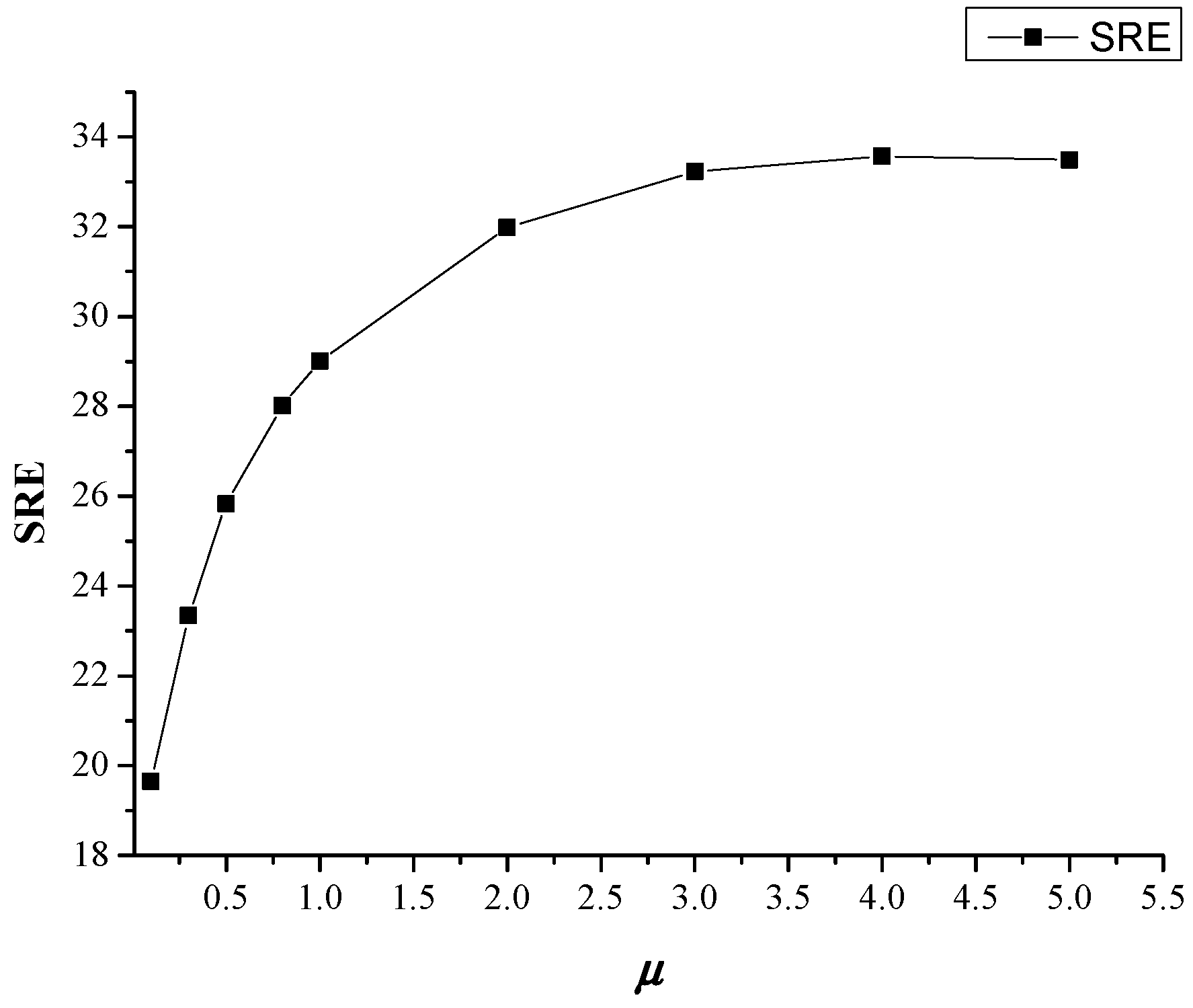
3.3.3. Discussion on Sensitivity Analysis for the Lagrangian Multiplier, μ
The Lagrangian multiplier μ is also an important inner parameter in solving the spatial regularization sparse unmixing algorithm with alternating direction method of multipliers (ADMM) strategy. To better understand the effect of the Lagrangian multiplier, we have also analyzed the selection of the Lagrangian multiplier parameter μ with simulated dataset 1. The quantitative results measured by SRE dB values that are obtained with different values of μ for RGSU are shown in Figure 13.
It can be noticed from Figure 13 that the SRE dB values are the highest when μ is set as 4, as compared with the other values. For simulated dataset 1, the performance of RGSU algorithm seems poorly when μ is set as a small value, such as 0.1 or 0.3. In the experimental settings, to achieve a good result, multiple attempts should be made according to the feedbacks.
4. Conclusions
In this paper, a Rolling Guidance based Sparse Unmixing algorithm, namely RGSU, has been proposed for hyperspectral remote sensing imagery. In RGSU, a scale-aware spatial regularization model, the rolling guidance spatial consideration method is designed as the spatial regularization term to utilize the extraction or recovery of spatial information in the unmixing procedure. Differing from the previous spatial regularization based sparse unmixing methods, such as TV-based sparse unmixing or the nonlocal sparse unmixing method, RGSU considers the different levels of details by controlling the structure and outlier removal and the edge/detail recovery. This method combines a Gaussian filter-like approach to realize the small-scale structure removal and a joint bilateral filtering process to account for the spatial domain and range domain correlations. The experimental results that are obtained using both simulated datasets and real hyperspectral images confirm the effectiveness of the proposed algorithm, which outperforms the other spatial regularization based methods in controlling the different scales of spatial information. RGSU can obtain better visual effects, and a higher SRE quantitative evaluation result than the current state-of-the-art sparse unmixing algorithms.
Acknowledgments
The authors would like to thank the research group supervised by J. M. Bioucas-Dias and A. Plaza for sharing the simulated datasets and the source code of the latest sparse algorithms with the community, together with the free downloads of the AVIRIS image data. The author would also like to thank C. Li and J. Ma for sharing their latest sparse unmixing algorithm source code and their good suggestions as to how we could improve our paper. The author also highly appreciate the time and consideration of the editors and four anonymous referees for their constructive suggestions that greatly improved the paper. This work was supported by the Fundamental Research Funds for the Central Universities, China University of Geosciences (Wuhan) (grant No. CUG170625); and the National Natural Science Foundation of China (grant No. 41701429 and 41371344).
Author Contributions
All the authors made significant contributions to the work. Ruyi Feng, Wenjuan Lin and Yanfei Zhong designed the research, analyzed the results, and accomplished the validation work. Lizhe Wang provided advice for the preparation and revision of the paper.
Conflicts of Interest
The authors declare no conflict of interest. The founding sponsors had no role in the design of the study; in the collection, analyses, or interpretation of data; in the writing of the manuscript; and in the decision to publish the results.
References
- Tong, Q.; Xue, Y.; Zhang, L. Progress in hyperspectral remote sensing science and technology in China over the past three decades. IEEE J. Sel. Top. Appl. Earth Obs. Remote Sens. 2014, 7, 70–91. [Google Scholar] [CrossRef]
- Bioucas-Dias, J.M.; Plaza, A.; Camps-Valls, G.; Scheunders, P.; Nasrabadi, N.M.; Chanussot, J. Hyperspectral remote sensing data analysis and future challenges. IEEE Geosci. Remote Sens. Mag. 2013, 1, 6–36. [Google Scholar] [CrossRef]
- Plaza, A.; Benediktsson, J.A.; Boardman, J.W.; Brazile, J.; Bruzzone, L.; Camps-Valls, G.; Chanussot, J.; Fauvel, M.; Gamba, P.; Gualtieri, A.; et al. Recent advances in techniques for hyperspectral image processing. Remote Sens. Environ. 2009, 113, 110–122. [Google Scholar] [CrossRef]
- Ghasrodashti, E.K.; Karami, A.; Heylen, R.; Scheunders, P. Spatial resolution enhancement of hyperspectral images using spectral unmixing and Bayesian sparse representation. Remote Sens. 2017, 9, 154. [Google Scholar] [CrossRef]
- Xu, X.; Tong, X.; Plaza, A.; Zhong, Y.; Xie, H.; Zhang, L. Joint sparse sub-pixel mapping model with endmember variability for remote sensing imagery. Remote Sens. 2017, 9, 15. [Google Scholar] [CrossRef]
- Bioucas-Dias, J.M.; Plaza, A.; Dobigeon, N.; Parente, M.; Du, Q.; Gader, P.; Chanussot, J. Hyperspectral unmixing overview: Geometrical, statistical, and sparse regression-based approaches. IEEE J. Sel. Top. Appl. Earth Obs. Remote Sens. 2012, 5, 354–379. [Google Scholar] [CrossRef]
- Wei, Q.; Chen, M.; Tourneret, J.Y.; Godsill, S. Unsupervised nonlinear spectral unmixing based on a multilinear mixing model. IEEE Trans. Geosci. Remote Sens. 2017, 55, 4534–4544. [Google Scholar] [CrossRef]
- Iordache, M.D.; Bioucas-Dias, J.M.; Plaza, A. Sparse unmixing of hyperspectral data. IEEE Trans. Geosci. Remote Sens. 2011, 49, 2014–2039. [Google Scholar] [CrossRef]
- Heinz, D.C.; Chang, C.-I. Fully constrained least squares linear spectral mixture analysis method for material quantification in hyperspectral imagery. IEEE Trans. Geosci. Remote Sens. 2001, 39, 529–545. [Google Scholar] [CrossRef]
- Kizel, F.; Shoshany, M.; Netanyahu, A.S.; Even-Tzur, G.; Benediktsson, J.A. A stepwise analytical projected gradient descent search for hyperspectral unmixing and its code vectorization. IEEE Trans. Geosci. Remote Sens. 2017, 55, 4923–4925. [Google Scholar] [CrossRef]
- Xu, M.; Du, B.; Zhang, L. Spatial-spectral information based abundance-constrained endmember extraction methods. IEEE J. Sel. Top. Appl. Earth Obs. Remote Sens. 2014, 7, 2004–2015. [Google Scholar] [CrossRef]
- Williams, M.; Kerekes, J.P.; Aardt, J. Application of abundance map reference data for spectral unmixing. Remote Sens. 2017, 9, 793. [Google Scholar] [CrossRef]
- Ma, W.K.; Bioucas-Dias, J.M.; Tsung-Han, C.; Gillis, N.; Gader, P.; Plaza, A.; Ambikapathi, A.; Chong-Yung, C. A signal processing perspective on hyperspectral unmixing: Insights from remote sensing. IEEE Signal Process. Mag. 2014, 31, 67–81. [Google Scholar] [CrossRef]
- Ammanouil, R.; Ferrari, A.; Richard, C.; Mary, D. Blind and fully constrained unmixing of hyperspectral images. IEEE Trans. Image Process. 2014, 23, 5510–5518. [Google Scholar] [CrossRef] [PubMed]
- Qian, Y.; Xiong, F.; Zeng, S.; Zhou, J.; Tang, Y. Matrix-vector nonnegative tensor factorization for blind unmixing of hyperspectral imagery. IEEE Trans. Geosci. Remote Sens. 2017, 55, 1776–1792. [Google Scholar] [CrossRef]
- Jia, S.; Qian, Y. Spectral and spatial complexity-based hyperspectral unmixing. IEEE Trans. Geosci. Remote Sens. 2007, 45, 3867–3879. [Google Scholar]
- Lu, X.; Wu, H.; Yuan, Y.; Yan, P.; Li, X. Manifold regularized sparse NMF for hyperspectral unmixing. IEEE Trans. Geosci. Remote Sens. 2013, 51, 2815–2826. [Google Scholar] [CrossRef]
- Salehani, Y.E.; Gazor, S.; Kim, I.-K.; Yousefi, S. l0-norm sparse hyperspectral unmixing using arctan smoothing. Remote Sens. 2016, 8, 187. [Google Scholar] [CrossRef]
- Iordache, M.D.; Bioucas-Dias, J.M.; Plaza, A. Collaborative sparse regression for hyperspectral unmixing. IEEE Trans. Geosci. Remote Sens. 2014, 52, 341–354. [Google Scholar] [CrossRef]
- Iordache, M.D.; Bioucas-Dias, J.M.; Plaza, A.; Somers, B. MUSIC-CSR: Hyperspectral Unmixing via Multiple Signal Classification and Collaborative Sparse Regression. IEEE Trans. Geosci. Remote Sens. 2014, 52, 4364–4382. [Google Scholar] [CrossRef]
- Ma, Y.; Li, C.; Mei, X.; Liu, C.; Ma, J. Robust sparse hyperspectral umixing with l2,1-norm. IEEE Trans. Geosci. Remote Sens. 2017, 55, 1227–1239. [Google Scholar] [CrossRef]
- Boardman, J.W.; Kruse, F.A.; Green, R.O. Mapping target signatures via partial unmixing of AVIRIS data. In Proceedings of the Fifth Annual JPL Airborne Earth Science Workshop, Pasadena, CA, USA, 23–26 January 1995. [Google Scholar]
- Winter, M.E. N-FINDR: An algorithm for fast autonomous spectral end-member determination in hyperspectral data. Proc. SPIE 2003, 3753, 266–275. [Google Scholar]
- Nascimento, J.M.P.; Bioucas-Dias, J.M. Does independent component analysis play a role in unmixing hyperspectral data? IEEE Trans. Geosci. Remote Sens. 2005, 43, 175–187. [Google Scholar] [CrossRef]
- Miao, L.; Qi, H. Endmember extraction from highly mixed data using minimum volume constrained nonnegative matrix factorization. IEEE Trans. Geosci. Remote Sens. 2007, 45, 765–777. [Google Scholar] [CrossRef]
- Zhong, Y.; Wang, X.; Zhao, L.; Feng, R.; Zhang, L.; Xu, Y. Blind spectral unmixing based on sparse component analysis for hyperspectral remote sensing imagery. ISPRS J. Photogramm. Remote Sens. 2016, 119, 49–63. [Google Scholar] [CrossRef]
- Bioucas-Dias, J.M.; Figueiredo, M. Alternating direction algorithms for constrained sparse regression: Application to hyperspectral unmixing. In Proceedings of the 2nd IEEE GRSS Workshop on Hyperspectral Image and Signal Processing: Evolution in Remote Sensing (WHISPERS), Reykjavik, Iceland, 14–16 June 2010. [Google Scholar]
- Iordache, M.D.; Bioucas-Dias, J.M.; Plaza, A. Total variation spatial regularization for sparse hyperspectral unmixing. IEEE Trans. Geosci. Remote Sens. 2012, 50, 4484–4502. [Google Scholar] [CrossRef]
- Zhong, Y.; Feng, R.; Zhang, L. Non-local sparse unmixing for hyperspectral remote sensing imagery. IEEE J. Sel. Top. Appl. Earth Obs. Remote Sens. 2014, 7, 1889–1909. [Google Scholar] [CrossRef]
- Altmann, Y.; Pereyra, M.; Bioucas-Dias, J.M. Collaborative sparse regression using spatially correlated supports-application to hyperspectral unmixing. IEEE Trans. Image Process. 2015, 24, 5800–5811. [Google Scholar] [CrossRef] [PubMed]
- Li, C.; Ma, Y.; Mei, X.; Liu, C.; Ma, J. Hyperspectral unmixing with robust collaborative sparse regression. Remote Sens. 2016, 8, 588. [Google Scholar] [CrossRef]
- Feng, R.; Zhong, Y.; Zhang, L. Adaptive spatial regularization sparse unmixing strategy based on joint MAP for hyperspectral remote sensing imagery. IEEE J. Sel. Top. Appl. Earth Obs. Remote Sens. 2016, 9, 5791–5805. [Google Scholar] [CrossRef]
- Rudin, L.; Osher, S.; Fatemi, E. Nonlinear total variation based noise removal algorithm. Phys. D 1992, 60, 259–268. [Google Scholar] [CrossRef]
- Haralick, R.M.; Sternbery, S.R.; Zhuang, X. Image analysis using mathematical morphology. IEEE Trans. Pattern Anal. Mach. Intell. 1987, PAMI-9, 532–550. [Google Scholar] [CrossRef]
- Buades, A.; Coll, B.; Morel, J.M. A non-local algorithm for image denoising. Proc. IEEE Conf. Comput. Vis. Pattern Recognit. 2005, 2, 60–65. [Google Scholar]
- Zhang, Q.; Shen, X.; Xu, L.; Jia, J. Rolling guidance filter. Proc. Eur. Conf. Comput. Vis. 2014, 8691, 815–830. [Google Scholar]
- Xia, J.; Bombrun, L.; Adali, T.; Berthoumieu, Y.; Germain, C. Classification of hyperspectral data with ensemble of subspace ICA and edge-preserving filtering. In Proceedings of the 2016 IEEE International Conference on Acoustics, Speech and Signal Processing, Shanghai, China, 20–25 March 2016. [Google Scholar]
- Lillo-Saavedra, M.; Gonzalo-Martin, C.; Garcia-Pedrero, A.; Lagos, O. Scale-aware pansharpening algorithm for agricultural fragmented landscapes. Remote Sens. 2016, 8, 870. [Google Scholar] [CrossRef]
- Wang, P.; Fu, X.; Tong, X.; Liu, S.; Guo, B. Rolling guidance normal filter for geometric processing. ACM Trans. Graphics (TOG) 2015, 34, 173. [Google Scholar] [CrossRef]
- Feng, R.; Zhong, Y.; Zhang, L. Adaptive non-local Euclidean medians sparse unmixing for hyperspectral imagery. ISPRS J. Photogramm. Remote Sens. 2014, 97, 9–24. [Google Scholar] [CrossRef]
- Li, X.; Wang, G. Optimal band selection for hyperspectral data with improved differential evolution. J. Ambient Intel. Hum. Comput. 2015, 6, 675–688. [Google Scholar] [CrossRef]
- Pan, S.; Wu, J.; Zhu, X.; Zhang, C. Graph ensemble boosting for imbalanced noisy graph stream classification. IEEE Trans. Cybern. 2015, 45, 954–968. [Google Scholar]
- Wang, L.; Song, W.; Liu, P. Link the remote sensing big data to the image features via wavelet transformation. Cluster Comput. 2016, 19, 793–810. [Google Scholar] [CrossRef]
- Lindeberg, T. Scale-space theory: A basic tool for analyzing structures at different scales. J. Appl. Stat. 1994, 21, 225–270. [Google Scholar] [CrossRef]
- Tomasi, C.; Manduchi, R. Bilateral filtering for grey and color images. In Proceedings of the Sixth International Conference on Computer Vision, Bombay, India, 7 January 1998; pp. 839–846. [Google Scholar]
- Kang, X.; Li, S.; Benediktsson, A. Spectral-spatial hyperspectral image classification with edge-preserving filtering. IEEE Trans. Geosci. Remote Sens. 2014, 52, 2666–2677. [Google Scholar] [CrossRef]
- Wu, J.; Wu, B.; Pan, S.; Wang, H.; Cai, Z. Locally weighted learning: How and when does it work in bayesian networks? Int. J. Comput. Int. Sys. 2015, 8, 63–74. [Google Scholar] [CrossRef]
- Wu, J.; Pan, S.; Zhu, X.; Cai, Z.; Zhang, P.; Zhang, C. Self-adaptive attribute weighting for Naive Bayes classification. Expert Syst. Appl. 2015, 42, 1478–1502. [Google Scholar] [CrossRef]
- Li, C.; Ma, Y.; Mei, X.; Fan, F.; Huang, J.; Ma, J. Sparse unmixing of hyperspectral data with noise level estimation. Remote Sens. 2017, 9, 1166. [Google Scholar] [CrossRef]
- Iordache, M.D. A Sparse Regression Approach to Hyperspectral Unmixing. Ph.D. Thesis, School of Electrical and Computer Engineering, Ithaca, NY, USA, 2011. [Google Scholar]
- Xu, X.; Zhong, Y.; Zhang, L.; Zhang, H. Sub-pixel mapping based on a MAP model with multiple shifted hyperspectral imagery. IEEE J. Sel. Top. Appl. Earth Obs. Remote Sens. 2013, 6, 580–593. [Google Scholar] [CrossRef]
Figure 1.
Flowchart of the scale-aware rolling guidance method.

Figure 2.
Basic schematic of the proposed Rolling Guidance Sparse Unmixing (RGSU) method.

Figure 3.
True fractional abundances of simulated dataset 1. (a) Five spectra; (b) True abundance images.
Figure 3.
True fractional abundances of simulated dataset 1. (a) Five spectra; (b) True abundance images.
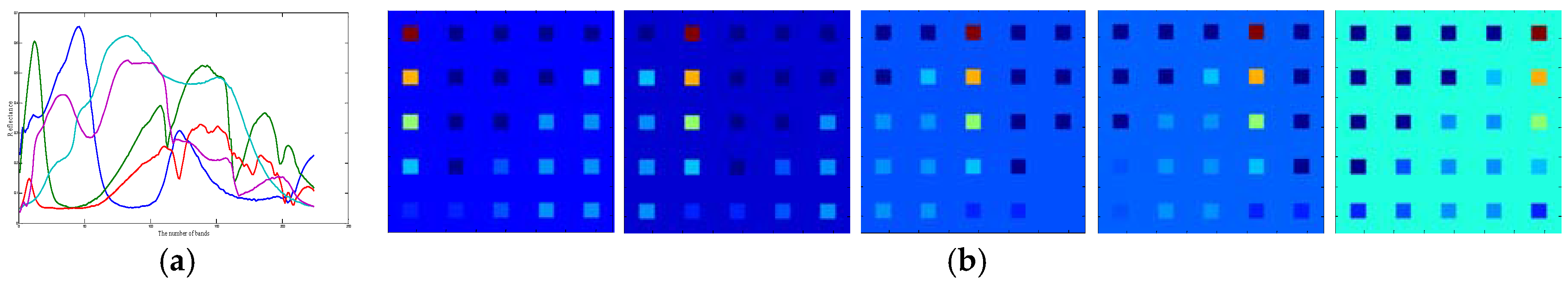
Figure 4.
True abundance maps of simulated dataset 2. (a) Endmember 1; (b) Endmember 2; (c) Endmember 3; (d) Endmember 4; (e) Endmember 5; (f) Endmember 6; (g) Endmember 7; (h) Endmember 8; (i) Endmember 9; and, (j) Spectral signatures.
Figure 4.
True abundance maps of simulated dataset 2. (a) Endmember 1; (b) Endmember 2; (c) Endmember 3; (d) Endmember 4; (e) Endmember 5; (f) Endmember 6; (g) Endmember 7; (h) Endmember 8; (i) Endmember 9; and, (j) Spectral signatures.
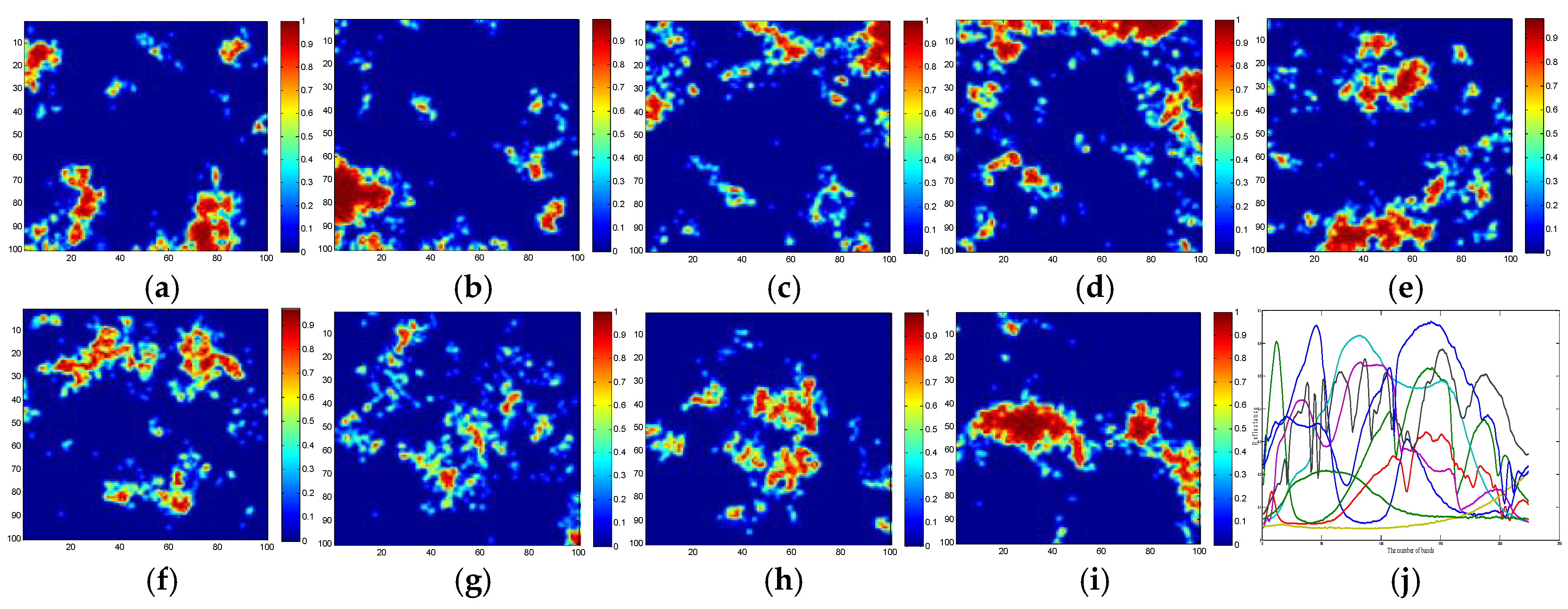
Figure 5.
Cuprite dataset. (a) Cuprite data; (b) United States Geological Survey (USGS) mineral spectral library.
Figure 5.
Cuprite dataset. (a) Cuprite data; (b) United States Geological Survey (USGS) mineral spectral library.

Figure 6.
Nuance data: (a) Nuance data; (b) Spectral_lib; (c) Higher-Resolution RGB image (HR) data; and (d) the approximate reference abundances, from left to right: dead leaves, fresh grass, background.
Figure 6.
Nuance data: (a) Nuance data; (b) Spectral_lib; (c) Higher-Resolution RGB image (HR) data; and (d) the approximate reference abundances, from left to right: dead leaves, fresh grass, background.

Figure 7.
Estimated abundances of endmembers 1, 2, and 5 for simulated dataset 1.
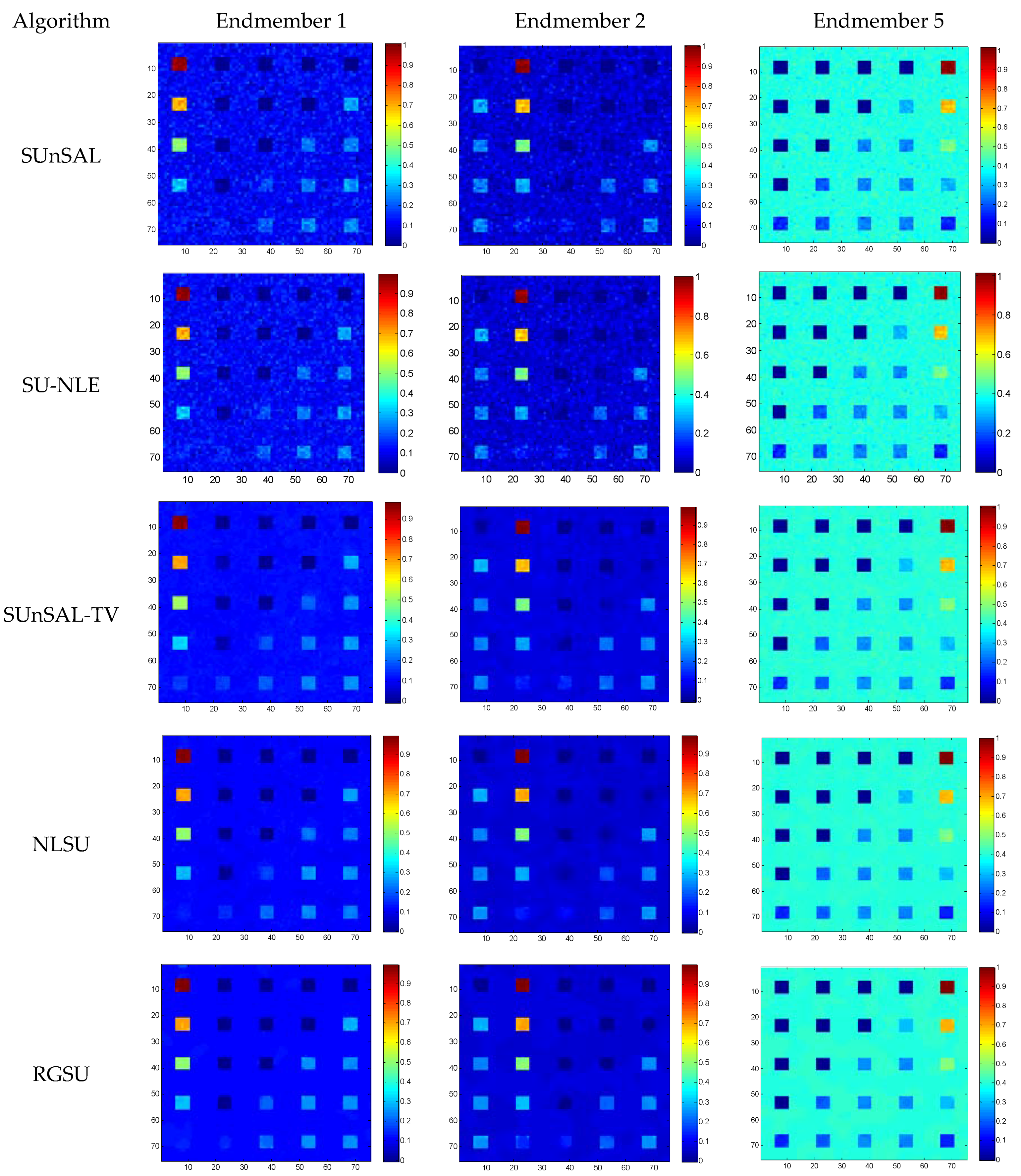
Figure 8.
Estimated abundances of endmembers 1, 2, and 5 for simulated dataset 2.

Figure 9.
Estimated abundances of alunite and buddingtonite for the Cuprite dataset.

Figure 10.
Estimated abundances of different components for the Nuance data.

Figure 11.
Signal-to-Reconstruction Error (SRE) (dB) values of RGSU with different combinations of inner parameters v and r.
Figure 11.
Signal-to-Reconstruction Error (SRE) (dB) values of RGSU with different combinations of inner parameters v and r.
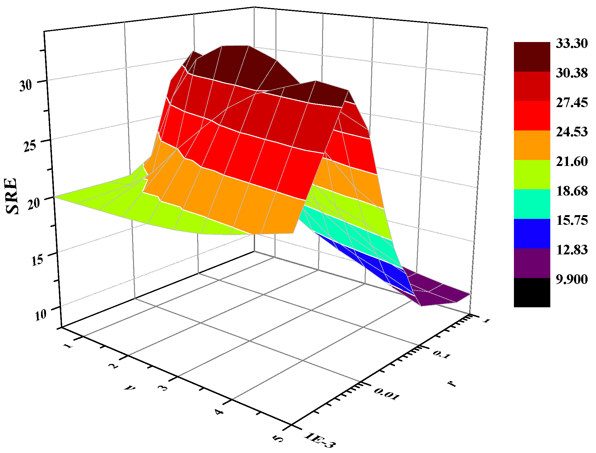
Figure 12.
Sensitivity analysis for regularization parameters λsps and λRG in RGSU algorithm with simulated dataset 1.
Figure 12.
Sensitivity analysis for regularization parameters λsps and λRG in RGSU algorithm with simulated dataset 1.

Figure 13.
Sensitivity analysis for the Lagrangian multiplier, μ in RGSU with simulated dataset 1.


Table 1.
Basic information about the four experimental datasets.
| Datasets | Simulated Dataset 1 | Simulated Dataset 2 | Cuprite Dataset | Nuance Data |
|---|---|---|---|---|
| Sensor | AVIRIS | AVIRIS | AVIRIS | Nuance NIR |
| Image size | 75 × 75 | 100 × 100 | 250 × 191 | 50 × 50 |
| Number of bands | 224 | 224 | 188 | 46 |
| SNR value (dB) | 30 | 30 | — | — |
Table 2.
Performance comparison for the different methods with the three datasets.
| Data | SUnSAL | SU-NLE | SUnSAL-TV | NLSU | RGSU | |
|---|---|---|---|---|---|---|
| Simulated dataset 1 | SRE (dB) | 15.1471 () | 15.7062 () | 25.8333 (;) | 29.6743 (;;;) | 33.3420 (;;;) |
| Time(s) | 0.4281 | 13.0313 | 30.4375 | 19.5000 | 47.5469 | |
| Simulated dataset 2 | SRE (dB) | 15.8856 () | 15.88 () | 18.7186 (;) | 21.3335 (;;;) | 23.4529 (;;;) |
| Time(s) | 2.7813 | 50.9219 | 62.7969 | 39.3750 | 88.5000 | |
| Nuance data | SRE (dB) | 4.9281 () | 4.8570 () | 5.3092 (;) | 6.0017 (;;;) | 6.0385 (;;;) |
| Time(s) | 2.9219 | 3.6563 | 4.4531 | 12.2188 | 24.3146 |
Note: The highest SRE values in the table are marked with bold.
© 2017 by the authors. Licensee MDPI, Basel, Switzerland. This article is an open access article distributed under the terms and conditions of the Creative Commons Attribution (CC BY) license (http://creativecommons.org/licenses/by/4.0/).
Share and Cite
MDPI and ACS Style
Feng, R.; Zhong, Y.; Wang, L.; Lin, W. Rolling Guidance Based Scale-Aware Spatial Sparse Unmixing for Hyperspectral Remote Sensing Imagery. Remote Sens. 2017, 9, 1218. https://doi.org/10.3390/rs9121218
AMA Style
Feng R, Zhong Y, Wang L, Lin W. Rolling Guidance Based Scale-Aware Spatial Sparse Unmixing for Hyperspectral Remote Sensing Imagery. Remote Sensing. 2017; 9(12):1218. https://doi.org/10.3390/rs9121218
Chicago/Turabian StyleFeng, Ruyi, Yanfei Zhong, Lizhe Wang, and Wenjuan Lin. 2017. "Rolling Guidance Based Scale-Aware Spatial Sparse Unmixing for Hyperspectral Remote Sensing Imagery" Remote Sensing 9, no. 12: 1218. https://doi.org/10.3390/rs9121218
Note that from the first issue of 2016, this journal uses article numbers instead of page numbers. See further details here.