TCCON Philippines: First Measurement Results, Satellite Data and Model Comparisons in Southeast Asia

 , , ,
, , ,  , and
, and
Abstract
:
1. Introduction
2. Materials and Methods
2.1. Site Description
2.2. Instrumentation
2.2.1. TCCON FTS
2.2.2. LiDAR System for GOSAT-2 Validation
2.3. GOSAT and OCO-2 Data
2.4. GEOS-Chem Tagged Tracer Simulations
2.5. Backward Trajectories
3. Results
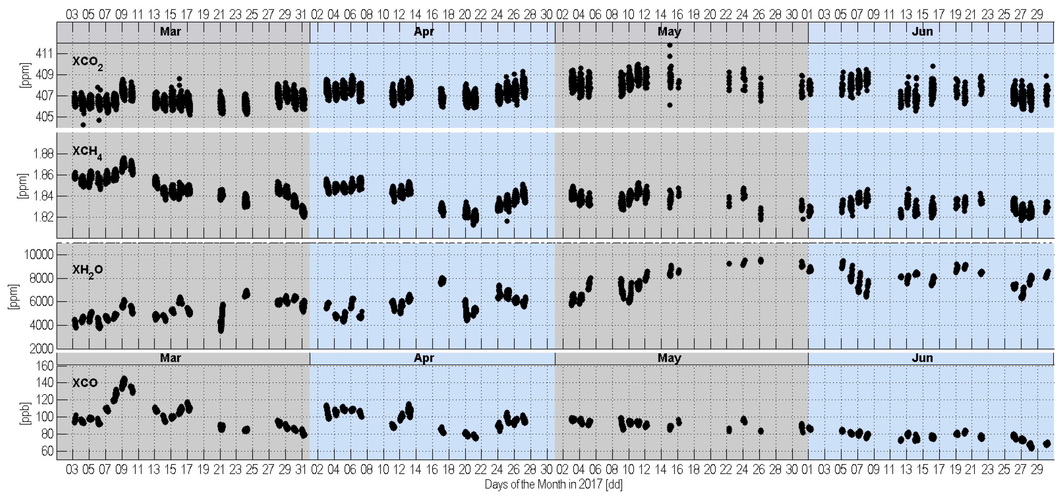
3.1. Time Series of , , and
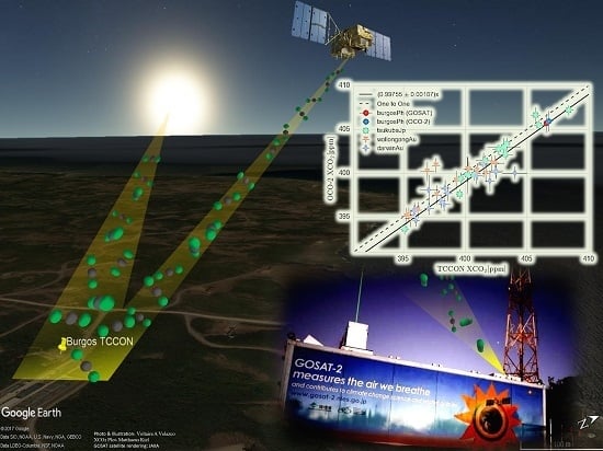
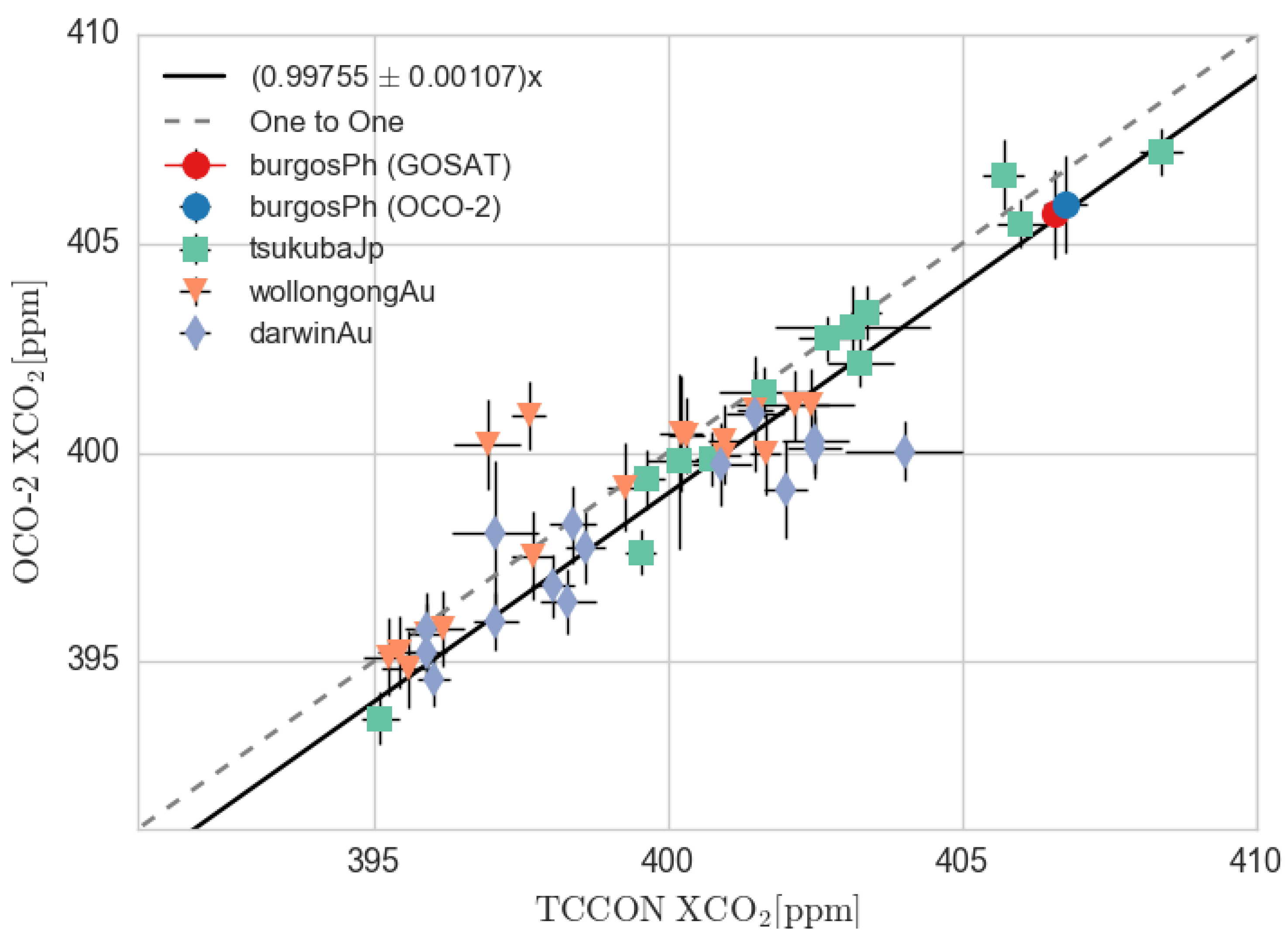
3.2. OCO-2, GOSAT and TCCON Comparisons
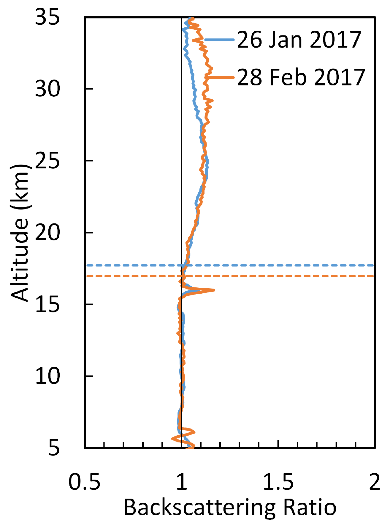
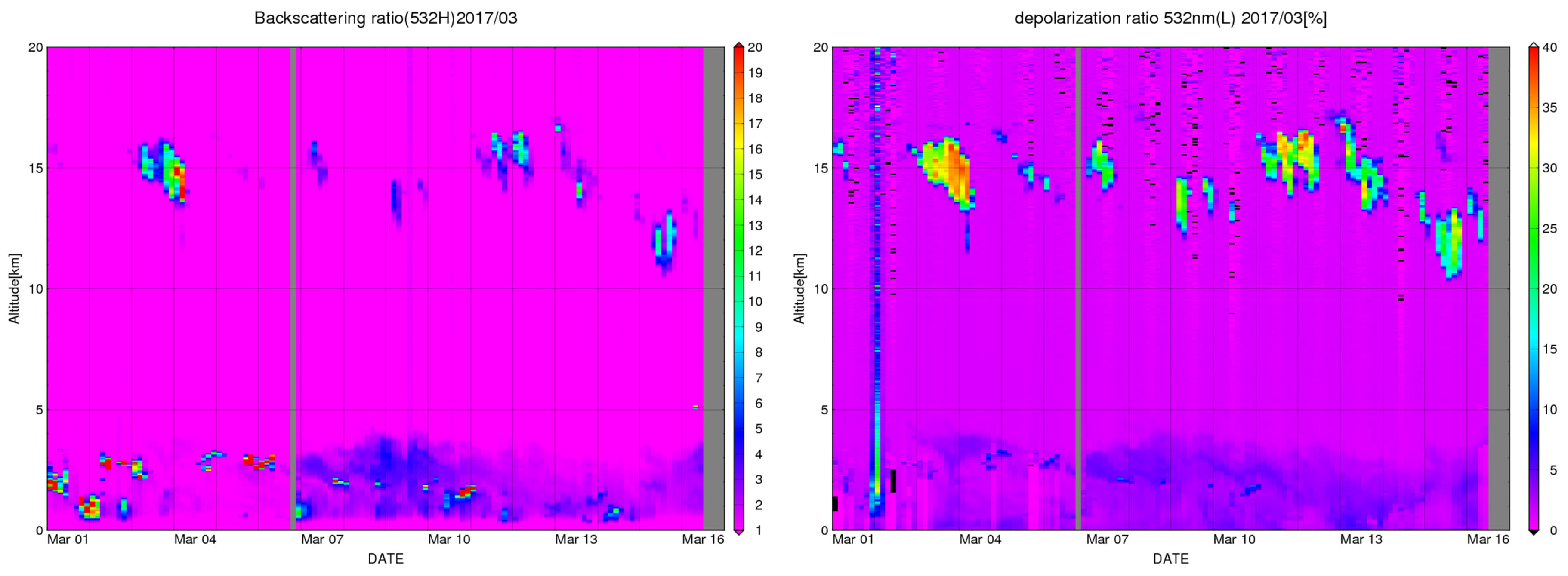
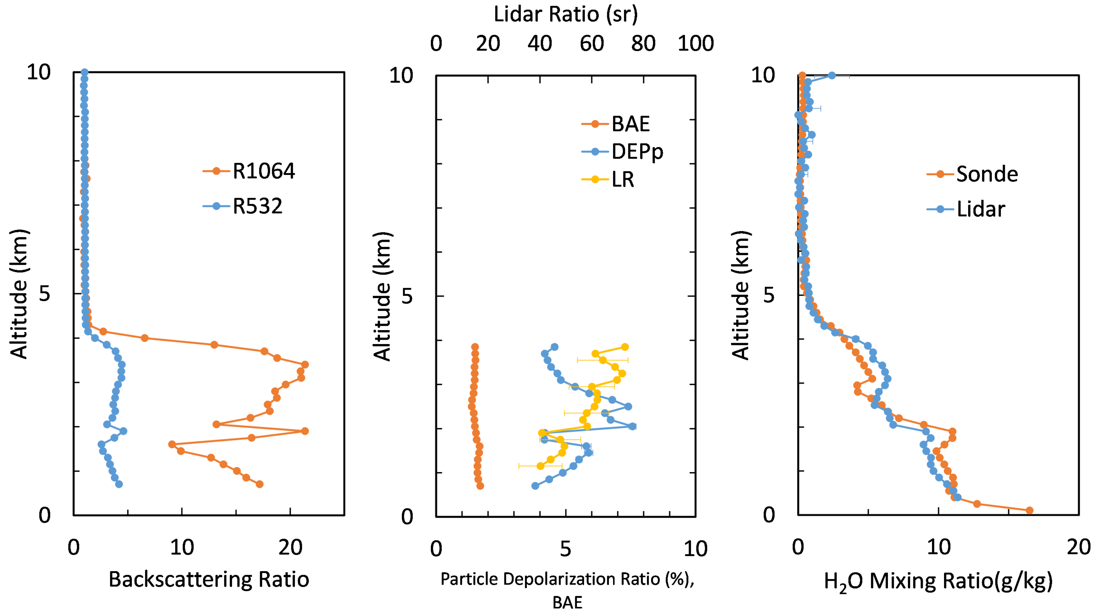
3.3. LiDAR Results
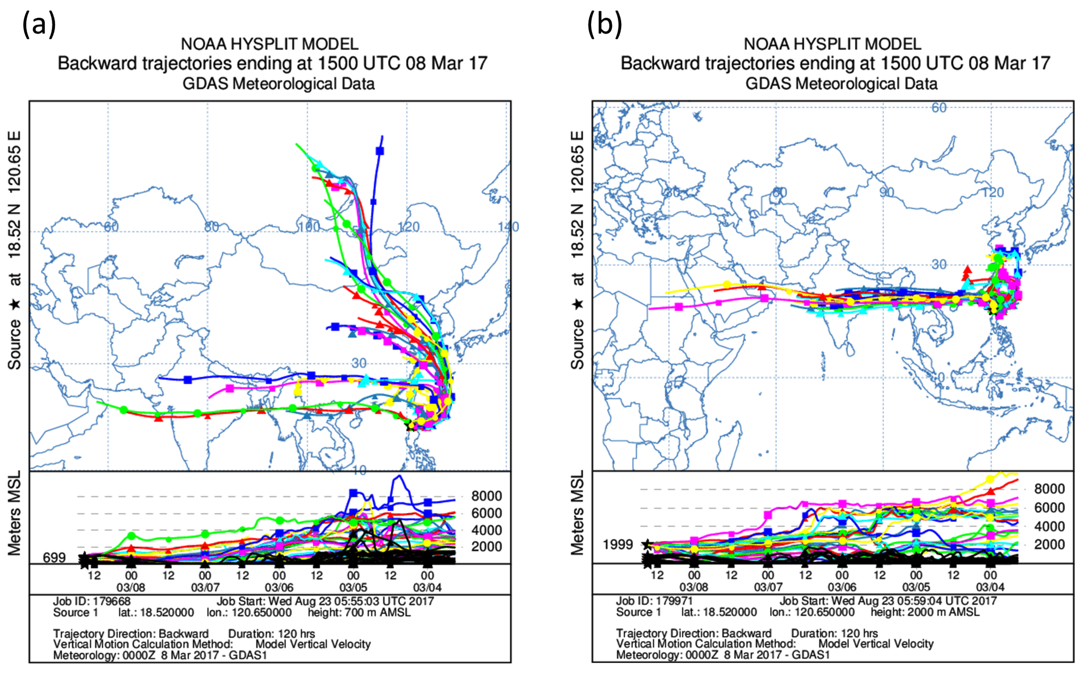
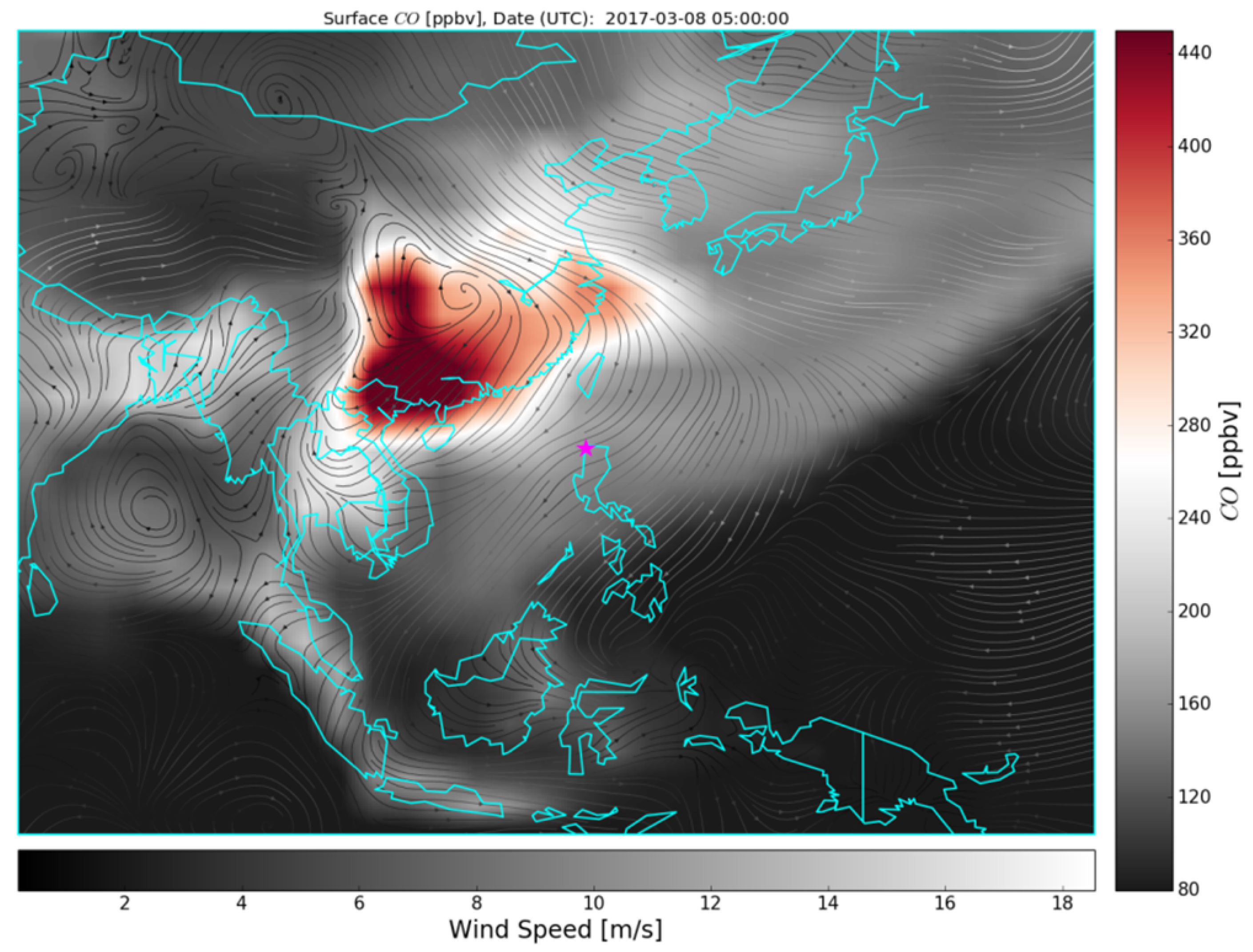
3.4. HYSPLIT Backward Trajectories
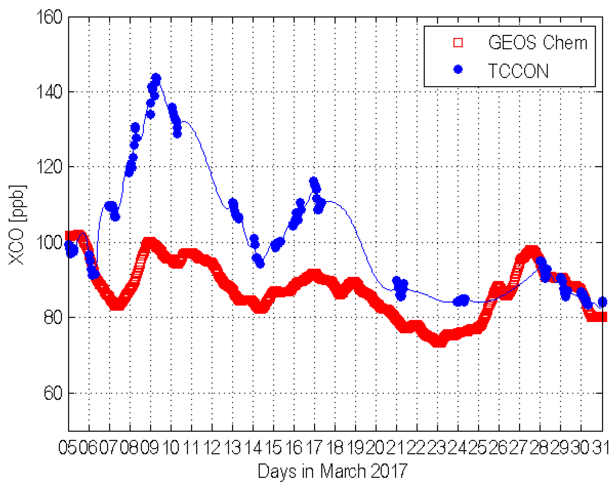
3.5. GEOS Chem Comparisons with TCCON Data
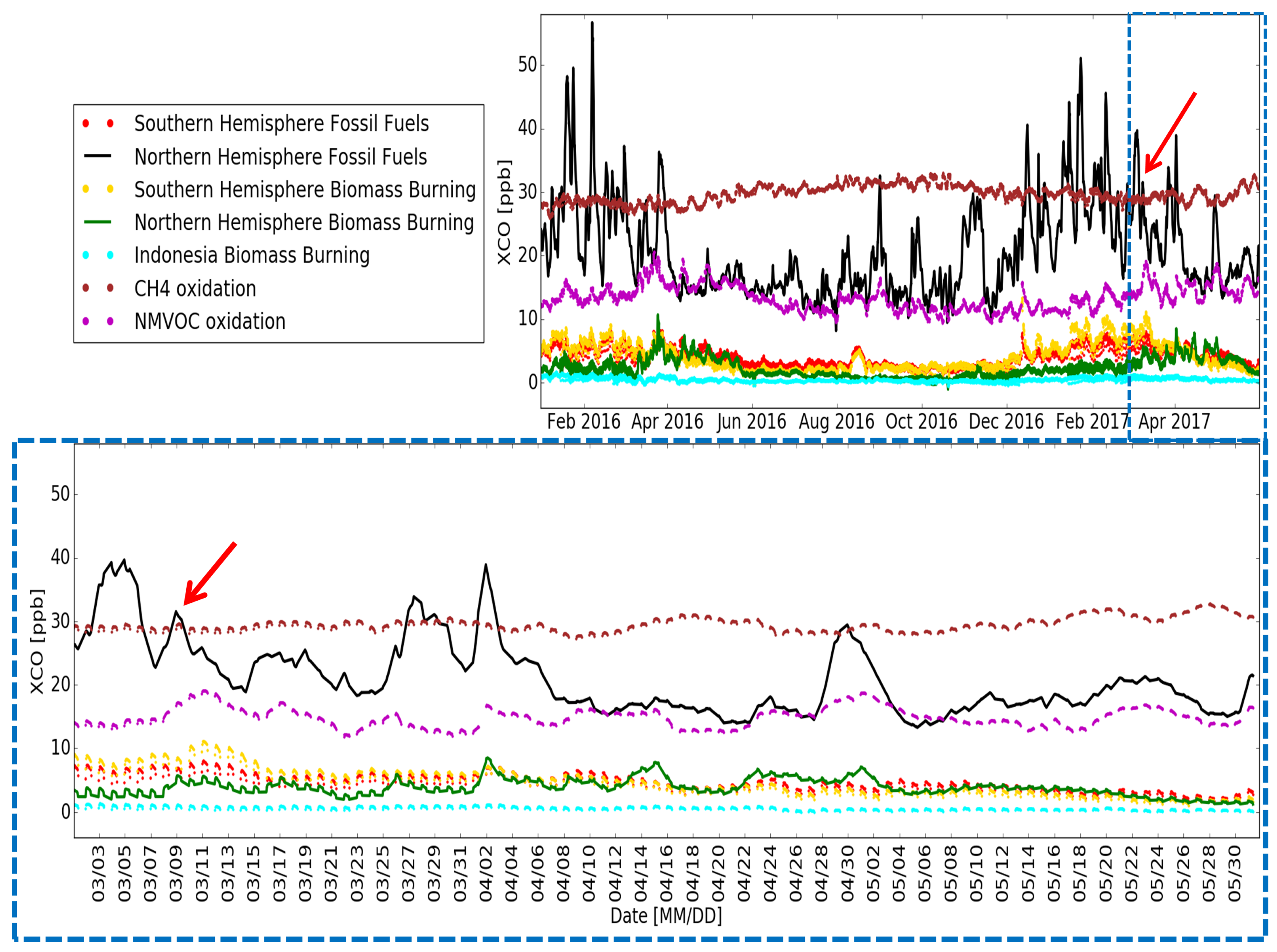
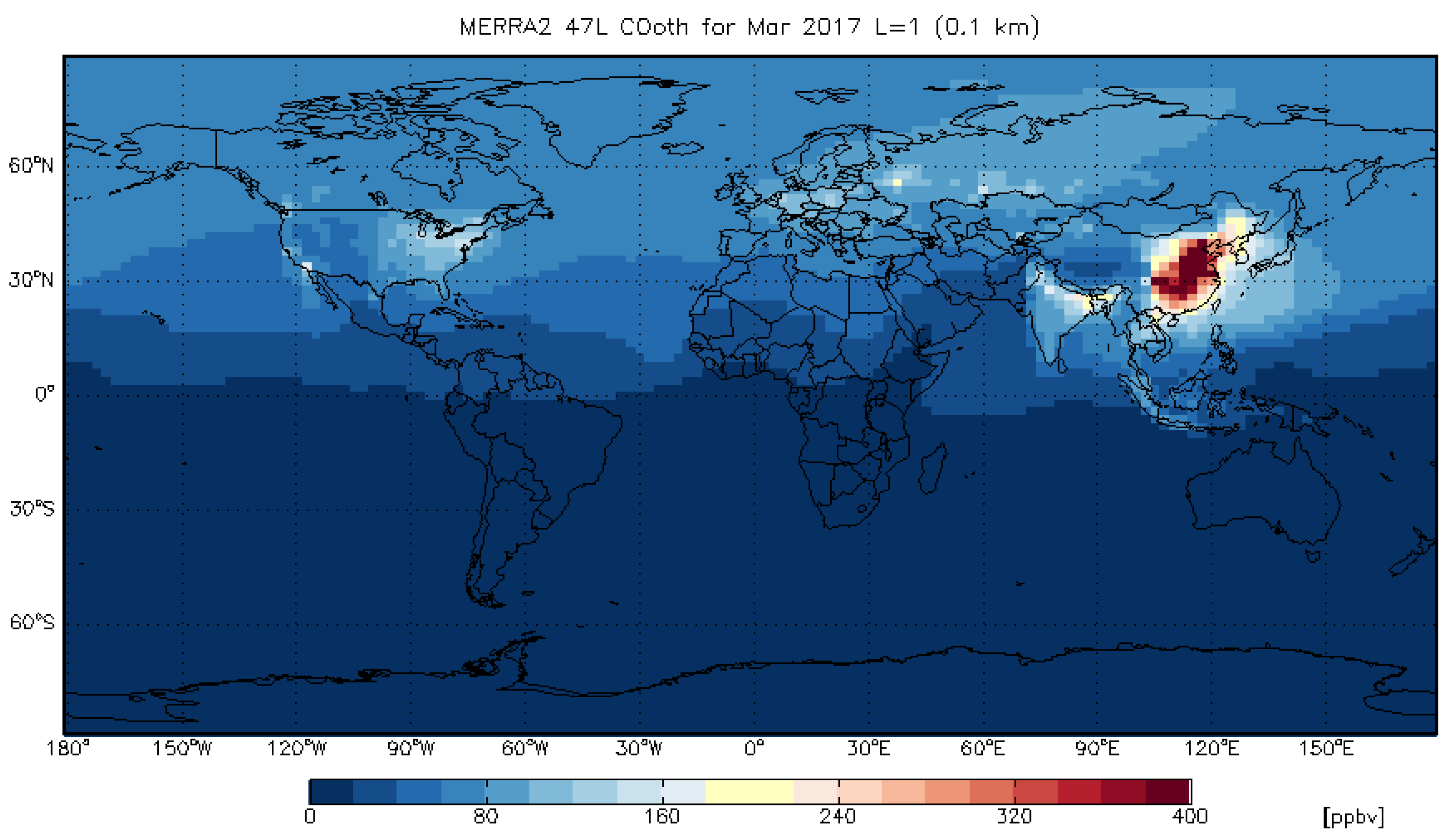
3.6. Tagged Tracer Simulations
4. Discussion
5. Conclusions
Acknowledgments
Author Contributions
Conflicts of Interest
References
- AccessScience. Available online: https://doi.org/10.1036/1097-8542.BR0612171 (accessed on 4 September 2017).
- Wunch, D.; Toon, G.C.; Blavier, J.F.L.; Washenfelder, R.A.; Notholt, J.; Connor, B.J.; Griffith, D.W.T.; Sherlock, V.; Wennberg, P.O. The Total Carbon Column Observing Network. Philos. Trans. R. Soc. A Math. Phys. Eng. Sci. 2011, 369, 2087–2112. [Google Scholar] [CrossRef] [PubMed]
- Kuze, A.; Suto, H.; Nakajima, M.; Hamazaki, T. Thermal and near infrared sensor for carbon observation Fourier-transform spectrometer on the Greenhouse Gases Observing Satellite for greenhouse gases monitoring. Appl. Opt. 2009, 48, 6716. [Google Scholar] [CrossRef] [PubMed]
- Nakajima, M.; Kuze, A.; Suto, H. The current status of GOSAT and the concept of GOSAT-2. In Sensors Systems, and Next-Generation Satellites XVI; Meynart, R., Neeck, S.P., Shimoda, H., Eds.; SPIE: Bellingham, WA, USA, 2012. [Google Scholar]
- Boesch, H.; Baker, D.; Connor, B.; Crisp, D.; Miller, C. Global characterization of CO2 column retrievals from Shortwave-Infrared Satellite Observations of the Orbiting Carbon Observatory-2 Mission. Remote Sens. 2011, 3, 270–304. [Google Scholar] [CrossRef]
- Eldering, A.; Kaki, S.; Crisp, D.; Gunson, M.R. The OCO-3 Mission. In Proceedings of the AGU Fall Meeting 2013, San Francisco, CA, USA, 9–13 December 2013. [Google Scholar]
- Ingmann, P.; Yasjka Meijer, B.V. Status overview of the GMES Missions Sentinel-4, Sentinel-5 and Sentinel-5p. In Proceedings of the ATMOS 2012—Advances in Atmospheric Science and Applications, Bruges, Belgium, 18–22 June 2012. [Google Scholar]
- Cressot, C.; Chevallier, F.; Bousquet, P.; Crevoisier, C.; Dlugokencky, E.J.; Fortems-Cheiney, A.; Frankenberg, C.; Parker, R.; Pison, I.; Scheepmaker, R.A.; et al. On the consistency between global and regional methane emissions inferred from SCIAMACHY, TANSO-FTS, IASI and surface measurements. Atmos. Chem. Phys. 2014, 14, 577–592. [Google Scholar] [CrossRef]
- Agency, I.E. Available online: http://www.iea.org/publications/freepublications/publication/WEO2015_SouthEastAsia.pdf (accessed on 4 September 2017).
- Rayner, P.J.; Utembe, S.R.; Crowell, S. Constraining regional greenhouse gas emissions using geostationary concentration measurements: A theoretical study. Atmos. Meas. Tech. 2014, 7, 3285–3293. [Google Scholar] [CrossRef]
- Velazco, V.; Morino, I.; Uchino, O.; Deutscher, N.; Bukosa, B.; Belikov, D.; Oishi, Y.; Nakajima, T.; Macatangay, R.; Nakatsuru, T.; et al. Total carbon column observing network Philippines: Toward quantifying atmospheric carbon in southeast asia. Clim. Disaster Dev. J. 2017, 2, 1–12. [Google Scholar] [CrossRef]
- Wunch, D.; Toon, G.C.; Sherlock, V.; Deutscher, N.M.; Liu, C.; Feist, D.G.; Wennberg, P.O. The Total Carbon Column Observing Network’s GGG2014 Data Version; Technical Report; Carbon Dioxide Information Analysis Center, Oak Ridge National Laboratory: Oak Ridge, TN, USA, 2015.
- Guerlet, S.; Butz, A.; Schepers, D.; Basu, S.; Hasekamp, O.P.; Kuze, A.; Yokota, T.; Blavier, J.F.; Deutscher, N.M.; Griffith, D.W.; et al. Impact of aerosol and thin cirrus on retrieving and validating XCO2 from GOSAT shortwave infrared measurements. J. Geophys. Res. Atmos. 2013, 118, 4887–4905. [Google Scholar] [CrossRef]
- Morino, I.; Uchino, O.; Inoue, M.; Yoshida, Y.; Yokota, T.; Wennberg, P.O.; Toon, G.C.; Wunch, D.; Roehl, C.M.; Notholt, J.; et al. Preliminary validation of column-averaged volume mixing ratios of carbon dioxide and methane retrieved from GOSAT short-wavelength infrared spectra. Atmos. Meas. Tech. 2011, 4, 1061–1076. [Google Scholar] [CrossRef]
- Uchino, O.; Kikuchi, N.; Sakai, T.; Morino, I.; Yoshida, Y.; Nagai, T.; Shimizu, A.; Shibata, T.; Yamazaki, A.; Uchiyama, A.; et al. Influence of aerosols and thin cirrus clouds on the GOSAT-observed CO2: A case study over Tsukuba. Atmos. Chem. Phys. 2012, 12, 3393–3404. [Google Scholar] [CrossRef]
- Yoshida, Y.; Kikuchi, N.; Morino, I.; Uchino, O.; Oshchepkov, S.; Bril, A.; Saeki, T.; Schutgens, N.; Toon, G.C.; Wunch, D.; et al. Improvement of the retrieval algorithm for GOSAT SWIR XCO2 and XCH4 and their validation using TCCON data. Atmos. Meas. Tech. 2013, 6, 1533–1547. [Google Scholar] [CrossRef]
- Ohyama, H.; Kawakami, S.; Tanaka, T.; Morino, I.; Uchino, O.; Inoue, M.; Sakai, T.; Nagai, T.; Yamazaki, A.; Uchiyama, A.; et al. Observations of XCO2 and XCH4 with ground-based high-resolution FTS at Saga Japan, and comparisons with GOSAT products. Atmos. Meas. Tech. 2015, 8, 5263–5276. [Google Scholar] [CrossRef]
- Zhou, M.; Dils, B.; Wang, P.; Detmers, R.; Yoshida, Y.; O’Dell, C.W.; Feist, D.G.; Velazco, V.A.; Schneider, M.; De Mazière, M. Validation of TANSO-FTS/GOSAT XCO2 and XCH4 glint mode retrievals using TCCON data from near-ocean sites. Atmos. Meas. Tech. 2016, 9, 1415–1430. [Google Scholar] [CrossRef]
- Eldering, A.; O’Dell, C.W.; Wennberg, P.O.; Crisp, D.; Gunson, M.R.; Viatte, C.; Avis, C.; Braverman, A.; Castano, R.; Chang, A.; et al. The Orbiting Carbon Observatory-2: First 18 months of science data products. Atmos. Meas. Tech. 2017, 10, 549–563. [Google Scholar] [CrossRef]
- Crisp, D.; Pollock, H.R.; Rosenberg, R.; Chapsky, L.; Lee, R.A.M.; Oyafuso, F.A.; Frankenberg, C.; O’Dell, C.W.; Bruegge, C.J.; Doran, G.B.; et al. The on-orbit performance of the Orbiting Carbon Observatory-2 (OCO-2) instrument and its radiometrically calibrated products. Atmos. Meas. Tech. 2017, 10, 59–81. [Google Scholar] [CrossRef]
- Zhao, C.L.; Tans, P.P. Estimating uncertainty of the WMO mole fraction scale for carbon dioxide in air. J. Geophys. Res. 2006, 111. [Google Scholar] [CrossRef]
- Wunch, D.; Toon, G.C.; Wennberg, P.O.; Wofsy, S.C.; Stephens, B.B.; Fischer, M.L.; Uchino, O.; Abshire, J.B.; Bernath, P.; Biraud, S.C.; et al. Calibration of the total carbon column observing network using aircraft profile data. Atmos. Meas. Tech. 2010, 3, 1351–1362. [Google Scholar] [CrossRef] [Green Version]
- Deutscher, N.M.; Griffith, D.W.T.; Bryant, G.W.; Wennberg, P.O.; Toon, G.C.; Washenfelder, R.A.; Keppel-Aleks, G.; Wunch, D.; Yavin, Y.; Allen, N.T.; et al. Total column XCO2 measurements at Darwin Australia: Site description and calibration against in situ aircraft profiles. Atmos. Meas. Tech. 2010, 3, 947–958. [Google Scholar] [CrossRef]
- Messerschmidt, J.; Geibel, M.C.; Blumenstock, T.; Chen, H.; Deutscher, N.M.; Engel, A.; Feist, D.G.; Gerbig, C.; Gisi, M.; Hase, F.; et al. Calibration of TCCON column-averaged CO2: the first aircraft campaign over European TCCON sites. Atmos. Meas. Tech. 2011, 11, 10765–10777. [Google Scholar]
- Mandrake, L.; O’Dell, C.W.; Wunch, D.; Wennberg, P.O.; Fisher, B.; Osterman, G.B.; Marchetti, Y.; Eldering, A. Orbiting Carbon Observatory-2 (OCO-2) Warn Level, Bias Correction, and Lite File Product Description; Technical Report; California Institute of Technology: Pasasdena, CA, USA, 2017. [Google Scholar]
- Wunch, D.; Wennberg, P.O.; Osterman, G.; Fisher, B.; Naylor, B.; Roehl, C.M.; O’Dell, C.; Mandrake, L.; Viatte, C.; Kiel, M.; et al. Comparisons of the Orbiting Carbon Observatory-2 (OCO-2) XCO2 measurements with TCCON. Atmos. Meas. Tech. 2017, 10, 2209–2238. [Google Scholar] [CrossRef]
- Fisher, J.A.; Murray, L.T.; Jones, D.B.A.; Deutscher, N.M. Improved method for linear carbon monoxide simulation and source attribution in atmospheric chemistry models illustrated using GEOS-Chem v9. Geosci. Model Dev. Discuss. 2017, 10, 4126–4144. [Google Scholar]
- European Commission. Emission Database for Global Atmospheric Research (EDGAR). Technical Report. Joint Research Centre (JRC)/Netherlands Environmental Assessment Agency (PBL): The Netherlands, 2011. Available online: http://edgar.jrc.ec.europa.eu/ (accessed on 30 October 2017).
- Li, M.; Zhang, Q.; Kurokawa, J.; Woo, J.H.; He, K.; Lu, Z.; Ohara, T.; Song, Y.; Streets, D.G.; Carmichael, G.R.; et al. MIX: A mosaic Asian anthropogenic emission inventory under the international collaboration framework of the MICS-Asia and HTAP. Atmos. Chem. Phys. 2017, 17, 935–963. [Google Scholar] [CrossRef]
- Vestreng, V.; Mareckova, K.; Kakareka, S.; Malchykhina, A.; Kukharchyk, T. Inventory Review 2007; Emission Data Reported to LRTAP Convention and NEC Directive; MSC-W Technical Report; UNFCCC: New York, NY, USA, 2007; Volume 1. [Google Scholar]
- Van Donkelaar, A.; Martin, R.V.; Pasch, A.N.; Szykman, J.J.; Zhang, L.; Wang, Y.X.; Chen, D. Improving the accuracy of daily satellite-derived ground-level fine aerosol concentration estimates for North America. Environ. Sci. Technol. 2012, 46, 11971–11978. [Google Scholar] [CrossRef] [PubMed]
- EPA, U.S. Available online:. Available online: http://www.epa.gov/ttnchie1/net/2005inventory.html (accessed on 27 November 2017).
- Kuhns, H.; Knipping, E.M.; Vukovich, J.M. Development of a United States–Mexico emissions inventory for the Big Bend Regional Aerosol and Visibility Observational (BRAVO) Study. J. Air Waste Manag. Assoc. 2005, 55, 677–692. [Google Scholar] [CrossRef] [PubMed]
- Yevich, R.; Logan, J.A. An assessment of biofuel use and burning of agricultural waste in the developing world. Glob. Biogeochem. Cycles 2003, 17. [Google Scholar] [CrossRef]
- Lee, C.; Martin, R.V.; van Donkelaar, A.; Lee, H.; Dickerson, R.R.; Hains, J.C.; Krotkov, N.; Richter, A.; Vinnikov, K.; Schwab, J.J. SO2 emissions and lifetimes: Estimates from inverse modeling using in situ and global, space-based (SCIAMACHY and OMI) observations. J. Geophys. Res. Atmos. 2011, 116. [Google Scholar] [CrossRef]
- Stettler, M.; Eastham, S.; Barrett, S. Air quality and public health impacts of UK airports. Part I: Emissions. Atmos. Environ. 2011, 45, 5415–5424. [Google Scholar] [CrossRef]
- Darmenov, A.; da Silva, A. The Quick Fire Emissions Dataset (QFED)–Documentation of Versions 2.1, 2.2 and 2.4; NASA Technical Report Series on Global Modeling and Data Assimilation, NASA TM-2013-104606; NASA: Washington, DC, USA, 2013; Volume 32, p. 183.
- Guenther, A.B.; Jiang, X.; Heald, C.L.; Sakulyanontvittaya, T.; Duhl, T.; Emmons, L.K.; Wang, X. The Model of Emissions of Gases and Aerosols from Nature version 2.1 (MEGAN2.1): An extended and updated framework for modeling biogenic emissions. Geosci. Model Dev. 2012, 5, 1471–1492. [Google Scholar] [CrossRef] [Green Version]
- Stein, A.F.; Draxler, R.R.; Rolph, G.D.; Stunder, B.J.B.; Cohen, M.D.; Ngan, F. NOAA’s HYSPLIT atmospheric transport and dispersion modeling system. Bull. Am. Meteorol. Soc. 2015, 96, 2059–2077. [Google Scholar] [CrossRef]
- Velazco, V.; Notholt, J.; Warneke, T.; Lawrence, M.; Bremer, H.; Drummond, J.; Schulz, A.; Krieg, J.; Schrems, O. Latitude and altitude variability of carbon monoxide in the Atlantic detected from ship-borne Fourier transform spectrometry model, and satellite data. J. Geophys. Res. 2005, 110. [Google Scholar] [CrossRef]
- Ridder, T.; Gerbig, C.; Notholt, J.; Rex, M.; Schrems, O.; Warneke, T.; Zhang, L. Ship-borne FTIR measurements of CO and O3 in the Western Pacific from 43°N to 35°S: An evaluation of the sources. Atmos. Chem. Phys. 2012, 12, 815–828. [Google Scholar] [CrossRef]
- O’Dell, C.W.; Eldering, A.; Crisp, D.; Fisher, B.; Gunson, M.; McDuffie, J.; Mandrake, L.; Smyth, M.; Wennberg, P.; Wunch, D. Recent Improvements in XCO2 Measurements from OCO-2. In Proceedings of the 13th International Workshop on Greenhouse Gas Measurements from Space, Helsinki, Finland, 6–8 June 2017; p. 54. [Google Scholar]
- Kobayashi, S.; Ota, Y.; Harada, Y.; Ebita, A.; Moriya, M.; Onoda, H.; Onogi, K.; Kamahori, H.; Kobayashi, C.; EndoO, H.; et al. The JRA-55 Reanalysis: General specifications and basic characteristics. J. Meteorol. Soc. Jpn. Ser. II 2015, 93, 5–48. [Google Scholar] [CrossRef]
- Uchino, O.; Sakai, T.; Izumi, T.; Nagai, T.; Morino, I.; Yamazaki, A.; Deushi, M.; Yumimoto, K.; Maki, T.; Tanaka, T.Y.; et al. LiDAR detection of high concentrations of ozone and aerosol transported from northeastern Asia over Saga Japan. Atmos. Chem. Phys. 2017, 17, 1865–1879. [Google Scholar] [CrossRef]
- Huang, R.J.; Zhang, Y.; Bozzetti, C.; Ho, K.F.; Cao, J.J.; Han, Y.; Daellenbach, K.R.; Slowik, J.G.; Platt, S.M.; Canonaco, F.; et al. High secondary aerosol contribution to particulate pollution during haze events in China. Nature 2014, 514, 218–222. [Google Scholar] [CrossRef] [PubMed] [Green Version]
- Reid, J.S.; Xian, P.; Hyer, E.J.; Flatau, M.K.; Ramirez, E.M.; Turk, F.J.; Sampson, C.R.; Zhang, C.; Fukada, E.M.; Maloney, E.D. Multi-scale meteorological conceptual analysis of observed active fire hotspot activity and smoke optical depth in the Maritime Continent. Atmos. Chem. Phys. 2012, 12, 2117–2147. [Google Scholar] [CrossRef] [Green Version]
- Lasco, R.D.; Lales, J.S.; Arnuevo, M.; Guillermo, I.Q.; de Jesus, A.C.; Medrano, R.; Bajar, O.F.; Mendoza, C.V. Carbon dioxide (CO2) storage and sequestration of land cover in the Leyte Geothermal Reservation. Renew. Energy 2002, 25, 307–315. [Google Scholar] [CrossRef]
- Suto, H.; Yajima, Y.; Nakajima, M. Airborne-Based Demonstration of Intelligent Pointing Onboard GOSAT-2. In Proceedings of the 13th International Workshop on Greenhouse Gas Measurements from Space, Helsinki, Finland, 6–8 June 2017; p. 87. [Google Scholar]
- Deutscher, N.M.; Sherlock, V.; Fletcher, S.E.M.; Griffith, D.W.T.; Notholt, J.; Macatangay, R.; Connor, B.J.; Robinson, J.; Shiona, H.; Velazco, V.A.; et al. Drivers of column-average CO2 variability at Southern Hemispheric Total Carbon Column Observing Network sites. Atmos. Chem. Phys. 2014, 14, 9883–9901. [Google Scholar] [CrossRef]
- Liu, H. Transport pathways for Asian pollution outflow over the Pacific: Interannual and seasonal variations. J. Geophys. Res. 2003, 108. [Google Scholar] [CrossRef]
- Bohren, C.F.; Huffman, D.R. Absorption and Scattering of Light by Small Particles; Wiley-VCH: Weinheim, Germany, 1983. [Google Scholar]
- Sakai, T.; Shibata, T.; Iwasaka, Y.; Nagai, T.; Nakazato, M.; Matsumura, T.; Ichiki, A.; Kim, Y.S.; Tamura, K.; Troshkin, D.; et al. Case study of Raman LiDAR measurements of Asian dust events in 2000 and 2001 at Nagoya and Tsukuba Japan. Atmos. Environ. 2002, 36, 5479–5489. [Google Scholar] [CrossRef]
- Velazco, V. LIDAR Studies of Water Vapor and Aerosols in the Boundary Layer in the Southern Hemisphere and in the Arctic. Master’s Thesis, University of Bremen, Bremen, Germany, 2002. [Google Scholar]
- Heese, B.; Baars, H.; Bohlmann, S.; Althausen, D.; Deng, R. Continuous vertical aerosol profiling with a multi-wavelength Raman polarization LiDAR over the Pearl River Delta China. Atmos. Chem. Phys. 2017, 17, 6679–6691. [Google Scholar] [CrossRef]
- Belikov, D.A.; Maksyutov, S.; Ganshin, A.; Zhuravlev, R.; Deutscher, N.M.; Wunch, D.; Feist, D.G.; Morino, I.; Parker, R.J.; Strong, K.; et al. Study of the footprints of short-term variation in XCO2 observed by TCCON sites using NIES and FLEXPART atmospheric transport models. Atmos. Chem. Phys. 2017, 17, 143–157. [Google Scholar] [CrossRef]


| Transmitter | ||||
|---|---|---|---|---|
| Laser | Nd:YAG | |||
| Wavelength | 532 nm | 1064 nm | ||
| Pulse energy | 210 mJ | 180 mJ | ||
| Pulse repetition rate | 10 Hz | |||
| Pulse width | 5 ns | 6 ns | ||
| Beam divergence | 0.1 mrad | 0.1 mrad | ||
| Receiver | ||||
| Telescope type | Advanced Coma-Free | |||
| Telescope diameter | 356 mm (f = 2845 mm) | |||
| Field of view | 1 mrad | |||
| Center wavelength | 532.05 nm | 1064.18 nm | 607.35 nm | 660.45 nm |
| Polarization | P and S | None | None | None |
| Number of channels | 3 | 1 | 1 | 1 |
| Interference filter | ||||
| Bandwidth (FWHM) | 0.32 nm | 0.38 nm | 0.25 nm | 0.3 nm |
| Transmission | 0.6 | 0.72 | 0.74 | 0.94 |
| Detectors | PMT | APD | PMT | PMT |
| (R3235-01) | (C30956EH) | (R3237-01MOD) | (R3237-01) | |
| Quantum efficiency | 0.08 | 0.68 | 0.06 | 0.04 |
| Signal processing | 16 bit A/D + Photon counting | |||
| Time resolution | 1 min | |||
| Range resolution | 7.5 m | |||
| Maximum Range | 120 km |
© 2017 by the authors. Licensee MDPI, Basel, Switzerland. This article is an open access article distributed under the terms and conditions of the Creative Commons Attribution (CC BY) license (http://creativecommons.org/licenses/by/4.0/).
Share and Cite
Velazco, V.A.; Morino, I.; Uchino, O.; Hori, A.; Kiel, M.; Bukosa, B.; Deutscher, N.M.; Sakai, T.; Nagai, T.; Bagtasa, G.; et al. TCCON Philippines: First Measurement Results, Satellite Data and Model Comparisons in Southeast Asia. Remote Sens. 2017, 9, 1228. https://doi.org/10.3390/rs9121228
Velazco VA, Morino I, Uchino O, Hori A, Kiel M, Bukosa B, Deutscher NM, Sakai T, Nagai T, Bagtasa G, et al. TCCON Philippines: First Measurement Results, Satellite Data and Model Comparisons in Southeast Asia. Remote Sensing. 2017; 9(12):1228. https://doi.org/10.3390/rs9121228
Chicago/Turabian StyleVelazco, Voltaire A., Isamu Morino, Osamu Uchino, Akihiro Hori, Matthäus Kiel, Beata Bukosa, Nicholas M. Deutscher, Tetsu Sakai, Tomohiro Nagai, Gerry Bagtasa, and et al. 2017. "TCCON Philippines: First Measurement Results, Satellite Data and Model Comparisons in Southeast Asia" Remote Sensing 9, no. 12: 1228. https://doi.org/10.3390/rs9121228