High Resolution Mapping of Cropping Cycles by Fusion of Landsat and MODIS Data


1
Guangdong Research Center of Smart Homeland Engineering, South China Normal University, Guangzhou 510631, China
2
State Key Laboratory of Earth Processes and Resource Ecology, Beijing Normal University, Beijing 100875, China
3
Ministry of Education Key Laboratory for Earth System Modeling, Department of Earth System Science, Tsinghua University, Beijing 100084, China
4
Guangdong Provincial Key Laboratory of Urbanization and Geo-simulation, Sun Yat-sen University, Guangzhou 510275, China
*
Authors to whom correspondence should be addressed.
Remote Sens. 2017, 9(12), 1232; https://doi.org/10.3390/rs9121232
Submission received: 9 November 2017
/
Revised: 23 November 2017
/
Accepted: 27 November 2017
/
Published: 29 November 2017
(This article belongs to the Special Issue Monitoring Agricultural Land-Use Change and Land-Use Intensity)
Abstract
:Multiple cropping, a common practice of intensive agriculture that grows crops multiple times in the agricultural land in one growing season, is an effective way to fulfill the food demand given limited cropland areas. Deriving cropping cycles from satellite data provides the spatial distribution of cropping intensities that allows for monitoring of the multiple cropping activities over large areas. Although efforts have been made to map cropping cycles at 500 m or coarser resolution, producing cropping cycle maps at high resolution remain challenging because data from single satellite sensor do not provide sufficient spatiotemporal observations. In this paper, we generate dense time series of satellite data at 30 m resolution by fusion of Landsat and MODIS data, and derive the cropping cycles from the fused time series data. The method achieves overall accuracies of 92.5% and 89.2%, respectively, for two typical regions of multiple cropping in China using samples identified based on satellite time series data, and an overall accuracy of 81.2% for four subregions using all samples identified based on multi-temporal high resolution images. The mapped crop cycles show to be reasonable geographically and agree with the national census data. The fusion approach provides a feasible way to map cropping cycles at 30 m resolution and enables improved depiction of the spatial distribution of multiple cropping.
1. Introduction
Agriculture in Asia provides over half of the world’s cereal with only one-third of cropland coverage [1,2,3]. To fulfill the food demand of large population, Asian countries often adopt intensive agriculture to increase grain production on limited cropland extents with heavy capital and labor inputs. Multiple cropping, a common practice of intensive agriculture that grows multiple crops in the same cropland during a single growing season, makes full use of the light-heat resources as well as other natural conditions to increase the agricultural production capacity [4,5,6]. Simultaneously, multiple cropping results in a series of subsequent environment and social issues, such as agricultural land use, water use and nutrient applications, cropland managements, and the reciprocal feedback of climate changes [7,8,9,10]. Information regarding the spatial distribution of multiple cropping is therefore essential for a wide range of applications and studies [11,12,13,14].
The spatiotemporal coverage provided by satellite remote sensing makes it an efficient and useful tool to monitor the activities of multiple cropping over large areas. Areas with multiple cropping exhibit cyclic patterns in time series of satellite-based vegetation indices, such as Normalized Difference Vegetation Index (NDVI) and Enhanced Vegetation Index (EVI), which reflect cropping activities on the ground. Identifying cropping cycles from satellite data allows for the characterization of multiple cropping from regional to continental scales. Yan et al. [15] analyzed the changes of multiple cropping intensities from 1980 to 1990s in China based on Advanced Very High Resolution Radiometer (AVHRR) time series at 8 km resolution. Ding et al. [16] derived maps of multiple cropping from the Global Inventory Modeling and Mapping Studies (GIMMS) time series data and analyzed the variation of multiple cropping in northern China from 1982 to 2012. With improved spatial resolution and data quality, Moderate Resolution Imaging Spectroradiometer (MODIS) time series have been used to derive the information of crop intensity at 250 m to 1000 m resolution. Li et al. [17] detected yearly cropping cycles in China based on smoothed MODIS EVI time series and validated the maps against national survey data at the province level. Estel et al. [18] mapped cropping systems in Europe using MODIS NDVI time series, which were found to agree with European agriculture management data. Gray et al. [3] used multi-temporal MODIS NBAR-EVI to map multiple cropping activities in Asia and produced reasonable results as validated at the provincial level. While mapping multiple cropping with satellite data at moderate and/or coarse resolutions has been extensively studied, there is a need to produce high-resolution maps of multiple cropping, simply because the pixel sizes at coarse resolution (from 0.5 to 8 km) are usually considerably larger than the actual field sizes of croplands [19], making their use difficult in downstream applications.
Challenges remain in terms of mapping cropping cycles at fine resolution over large areas. One reason is that data from a single satellite sensor are not capable of capturing the fast-changing cropping activities on the ground. The harvest and replantation of crops for multiple cropping could be completed within one month or two [20,21]. Unlike natural vegetation, crops often reach canopy maturation quickly after plantation and have a relatively short growing period. The agricultural lands with higher cropping intensities often have more fragmental patches because farmers tend to access and manage the croplands more frequently [22,23,24]. In essence, producing high-resolution maps of multiple cropping requires time series of satellite data at both high temporal and spatial resolutions. However, the spatial and temporal resolutions of satellite sensors are compromised. High resolution sensors like Landsat do not collect images frequently enough, whereas coarse resolution sensors like MODIS have sufficient temporal resolution but less than ideal spatial resolution [25]. To date, no individual satellite sensor has proven suitable for mapping cropping cycles at high spatial resolution.
Fortunately, methods have been developed for blending data from sensors at different spatiotemporal resolutions and produce dense time series of satellite images at high spatial resolution [26,27,28,29,30]. Gao et al. [31] proposed the algorithm of spatial and temporal adaptive reflectance fusion model (STARFM) to predict daily surface reflectance at Landsat spatial resolution and MODIS temporal frequency. The algorithm designed based on spectral difference, temporal difference and location distance has proven to be useful in forested areas and cropland regions. Zhu et al. [32] developed an enhanced version of the STARFM based on the spectral unmixing method to improve the fusion of surface reflectance data in heterogeneous landscape. Hilker et al. [33] introduced a spatial temporal adaptive algorithm for mapping reflectance change (STAARCH) using the Tasseled Cap transformation and generated dense time series of Landsat data through data blending with MODIS for mapping forest disturbance. Wu et al. [34] developed a spatial temporal data fusion approach (STDFA) and predicted the surface reflectance of fine resolution pixels. These studies have successfully produced time series of high-resolution images based on the fusion approach using data from different satellite sensors. The fusion method therefore provides a potential solution to mapping cropping cycles at high spatial resolution, but remains to be tested.
The main goal here is to propose a method to map cropping cycles at high resolution based on fusion of Landsat and MODIS data. The proposed method is applied to map cropping cycles in major agricultural regions in China. The efforts to develop such a method would allow for producing useful maps of cropping cycles at high resolution over large areas.
2. Materials
2.1. Study Area
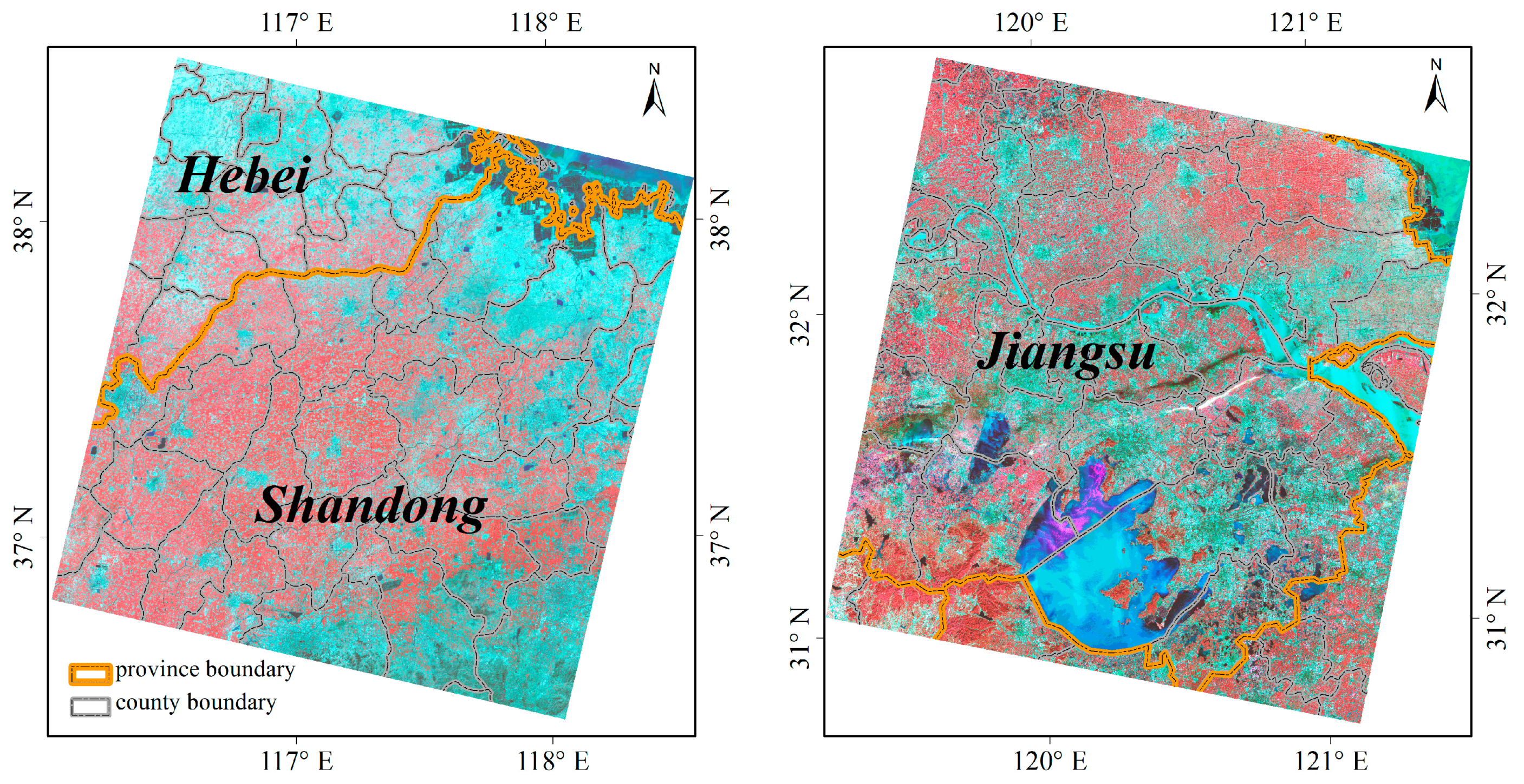
China has a long land use history to cultivate crops intensively. Two Landsat scenes that cover representative areas of multiple cropping in China were selected for study (Figure 1). One Landsat scene (Path 122 Row 034) crosses Shandong Province (hereinafter referred to as SD) and Hebei Province in the North China Plain, and the other (Path 119 Row 038) is located in Jiangsu Province (hereinafter referred to as JS) in the Yangtze Downstream Plain. Both scenes cover an area of approximately 170 × 180 km.
The SD scene covers southern Hebei Province and northern Shandong Province, which are both major grain producing provinces in China. The SD region has a warm temperate monsoon climate with abundant precipitation and heat resources. As the length of frost free season increases from northeast to southwest, there is a geographic transition of single cropping to double cropping from north to south. The region is typically cultivated in high intensity with relatively large field sizes. Winter wheat and maize are major crop types, whereas other planted crop types include soybean, barley, paddy rice, and sorghum.
The JS scene covers southern Jiangsu Province, another major grain producing province along the east coast of southern China. The JS region has a subtropical moist monsoon climate that is characterized by mild weather and moderate rainfall. Due to rapid economic growth and urban developments, the agricultural field size in JS is relatively small, making it difficult to derive information related to multiple cropping from coarse remote sensing data. For most of the multiple cropping activities, paddy rice and maize are planted in June and harvested in October, followed by crops such as winter wheat, barley, and rapeseed planted in November and harvested in the next June.
2.2. Data
The used datasets include 30 m Landsat 8 Operational Land Imager (OLI) images, 500 m MODIS surface reflectance products, 1000 m MODIS land surface temperature products, and 30 m land cover maps. Landsat 8 surface reflectance higher-level data products in 2015 were obtained from the Earth Resources Observation and Science (EROS) Center Science Processing Architecture (ESPA) website [35]. The Landsat 8 surface reflectance images delivered along with cloud mask data were generated from the Landsat Surface Reflectance Code (LaSRC). MODIS 8-day surface reflectance Version 6 products from both Terra and Aqua (MOD09A1 and MYD09A1) and MODIS 8-day land surface temperature Version 6 products (MOD11A2) in 2014–2016 were downloaded from the Land Processes Distributed Active Archive Center (LPDAAC) website [36]. The MODIS surface reflectance products along with ancillary quality control data that are indicative to the observation quality were delivered in the Sinusoidal projection at 500 m resolution. The MODIS land surface temperature products were provided in the Sinusoidal projection at 1000 m resolution. To match the spatial extents of the Landsat images, all MODIS products were resampled to 30 m resolution in the Universal Transverse Mercator (UTM) projection. The 30 m resolution land cover data of GlobeLand30 for the year of 2010 were obtained from the website of National Geomatics Center of China [37]. The classification system of GlobeLand30 includes 10 land cover types: cultivated land, forest, grassland, shrub land, wetland, water bodies, tundra, artificial surfaces, bare land, and permanent snow and ice [38]. The GlobeLand30 images are also reprojected using the Geospatial Data Abstraction Library (GDAL) tool to match the spatial extents of Landsat images. Multi-temporal very high-resolution images of GaoFen-1 (GF1, 2 m spatial resolution) and GaoFen-2 (GF2, 1 m spatial resolution) that were acquired during key phenophases of crop growth were sourced from China Center for Resources Satellite Data and Applications [39]. For the SD scene, the used images include GF-1 images acquired on 6 January, 29 March, 26 July and 20 October 2015 and GF-2 images acquired on 23 March, 26 April and 26 September 2105. For the JS scene, the used images include GF-1 images acquired on 24 March, 14 June, 29 July and 3 December 2015. All sourced GF images are almost cloud-free and have already been preprocessed with radiometric correction, geometric correction, and band fusion.
3. Methods
As improved based on our previous study [17], the method to map cropping cycles (Figure 2) involves three main steps as follows: (1) generating 8-day time series surface reflectance data at 30 m resolution based on fusion of Landsat and MODIS data; (2) deriving and smoothing fused EVI time series at 30 m resolution; and (3) extracting cropping cycles based on the smoothed fusion time series and refining mapped cropping cycles based on land surface temperature data and land cover maps.
3.1. Generating 8-Day 30 m Surface Reflectance Data by Fusion of Landsat and MODIS Data
Deriving high-resolution maps of cropping cycles from remotely sensed data requires time series observations that track cropping activities on the ground. While observations from Landsat have the high spatial resolution of 30 m, the temporal resolution of Landsat images is insufficient for tracking the dynamics of cropping activities, especially when accounting for the issue of cloud contamination. For example, there are only approximately 3–8 cloud-free Landsat images available in 2015 for both scenes (Table 1), whereas the activities of crop harvest and replantation could occur within 1–2 months. By comparison, MODIS provides observations with less than ideal spatial resolution (250 to 1000 m) and sufficient temporal resolution at a near daily basis. The 8-day composites of MODIS data (46 observations in a calendar year) have proven to reduce the effects of cloud contamination effectively and thus provide a suitable basis for capturing the variation of cropping phenology in many studies [40,41,42]. To combine the strength of Landsat and MODIS observations, we therefore applied a widely used method of the Spatial and Temporal Adaptive Reflectance Fusion Model (STARFM) to generate 8-day surface reflectance data at 30 m resolution [31].
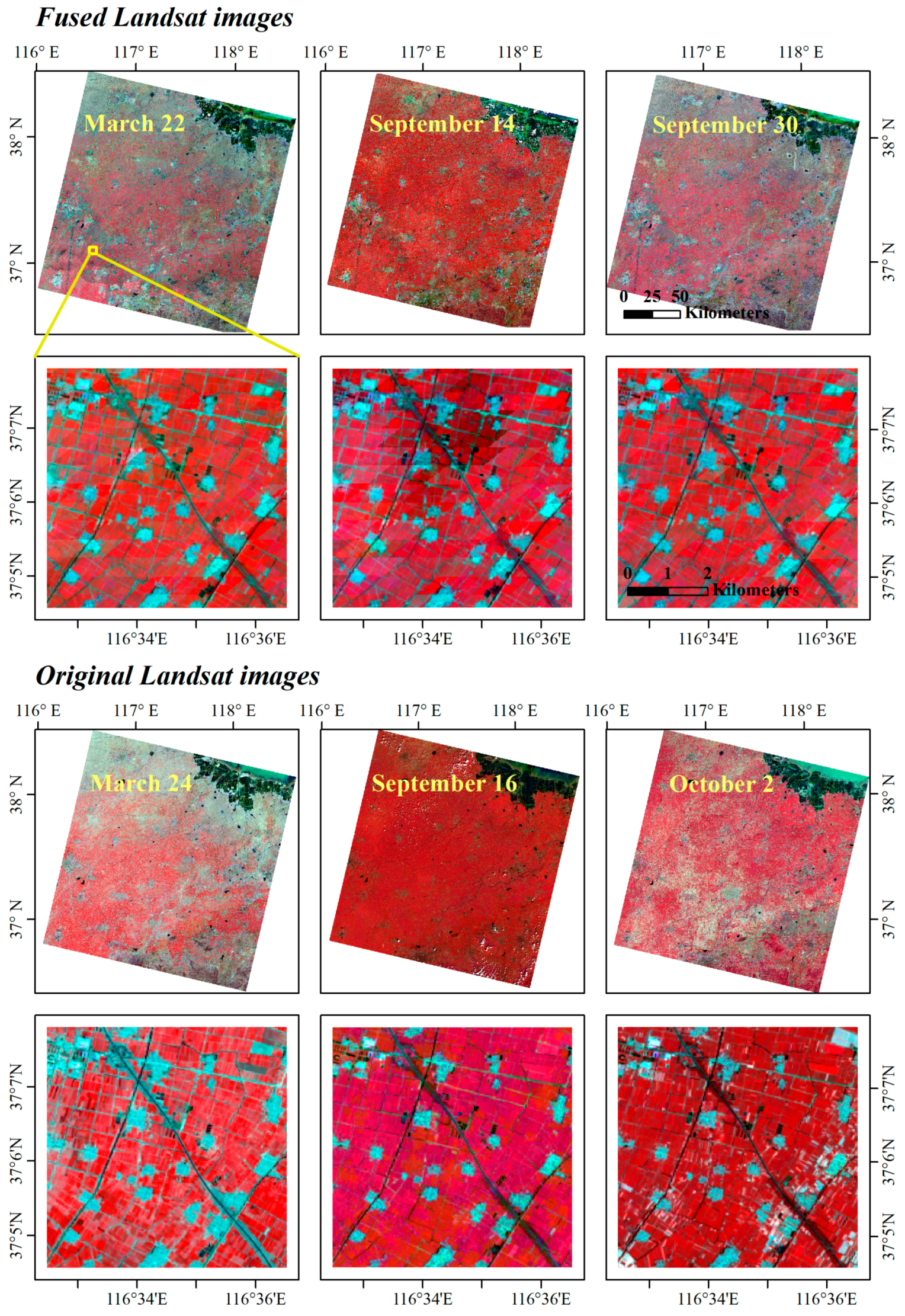
STARFM is a robust tool in generating high-resolution surface reflectance data using Landsat and MODIS images, and has found to achieve good performance over forest and crop areas. Here, we apply the STARFM algorithm to blend Landsat OLI surface reflectance images and MODIS 8-day surface reflectance data, which have already been preprocessed to account for atmospheric correction and screen out cloud contaminated pixels. For each scene, one clear and good quality image of Landsat OLI at the key phase of crop growth was selected as the fine-resolution image for fusion (i.e., the Landsat 8 image acquired on 25 April 2015 for the SD scene and the Landsat 8 image acquired on 13 October 2015 for the JS scene, respectively). The 8-day MODIS products that have the closest observation dates with the Landsat images were chosen as the matched coarse-resolution image, supposing that the differences of the acquisition time between Landsat and MODIS input data are negligible. The entire time series of MODIS surface reflectance data from 2014 to 2016 were then used to generate the 30 m 8-day surface reflectance data separately for both the Terra and Aqua products. To deriving EVI time series data, the near-infrared, red, and blue bands (Landsat OLI band 5, 4, and 2, and MODIS band 2, 1, and 3, respectively) were processed with false-color-composite images shown in Figure 3 as examples. Based on visual examination, STARFM could evidently generate reasonable images at both high spatial and temporal resolutions by dealing with the effects of land cover mixtures at MODIS resolutions.
3.2. Deriving and Smoothing High-Resolution EVI Time Series
Because EVI has proven in capturing vegetation dynamics with improved sensitivity as compared to NDVI, the surface reflectance data from both MODIS Terra and Aqua are used to derive EVI based on the following equation [43] and then further synthesized based on the minimum blue compositing method:
Note that, although MODIS vegetation indices products are provided from the website of LPDAAC, the EVI time series are produced on a 16-day basis, which is insufficient to capture rapid temporal variation in crop growth [44,45,46,47,48]. More importantly, to derive high-resolution EVI data correctly, it is needed to apply surface reflectance data rather than non-linear indices of EVI to the algorithm of STARFM.
There is a need to process the fused EVI time series with appropriate smoothing methods because the fused EVI time series as generated from the MODIS 8-day composite data could contain a certain degree of noise originated from sources such as atmospheric contamination and viewing and illumination angles. The software of TIMESAT is used to produce smoothed EVI time series for the identification of cropping cycles. TIMESAT provides three fitting algorithms, including asymmetric Gaussian, double logistic, and adaptive Savitzky–Golay. Based on the findings of previous studies [17], we applied the filter of adaptive Savitzky–Golay to the fused EVI time series. To preserve the subtle information of crop phenology variation, we applied the second-order polynomial and the window size of 4 for the 8-day composite data (i.e., 32-days).
Typical points of different cropping cycles are shown in Figure 4 as examples to illustrate the processes of the time series fitting, where cloudy observations as identified based on the original MODIS quality control data were assigned small weights in the fitting function. As seen in Figure 4, EVI time series well track the dynamics of crop growth during the growing season, as EVI first increases after the plantation of crops, peaks at the time of crop maturation, and then decreases after crops are harvested. Single cropping exhibits only one periodic cycle in the calendar year. Double cropping could have two or three peaks during the calendar year, because the plantation of winter wheat in November typically results in another peak of EVI in November or December right before the dormancy of winter wheat during the winter time. Fallow areas could also have a periodic cycle in the growing season, but the peak value of EVI is often low. The fitted EVI time series data at 30 m resolution then serve as the basis for identifying the numbers of the periodic cropping cycles in a calendar year.
3.3. Mapping Cropping Cycles Based on Fusion EVI
To extract the growing cycles from time series of satellite data, studies have developed different algorithms [49,50,51,52]. The complete detail of the used method is described in our previous work [17], and here we summarize it briefly.
Mapping cropping cycles from analysis of EVI time series involves major steps as follows. First, local maxima and minima in the fitted EVI time series are detected as potential peaks and troughs, respectively, by applying a centered moving window of 9, which is equivalent to 32 days before and after the centered observation. Second, spurious peaks of time series with EVI less than 0.35 are discarded because the EVI values of croplands, if planted, generally exceed 0.40 at maturation. Third, to make peaks and troughs alternate in the time series and to reduce influence of occasional undetected clouds, potential peaks and troughs are checked iteratively where successive potential peaks with no intervening trough are merged by keeping observations with higher EVI. Fourth, the numbers of cropping cycles are counted based on the numbers of peaks for the calendar year. Fifth, we apply a conservative minimum threshold of 5 °C based on the nighttime land surface temperature of MODIS products (MOD11A2) to define the start and the end of a growing season in a year, and deduct the number of cropping cycles if one peak falls in the non-growing season in order to account for the false peak resulted by the plantation of winter wheat. Last, the mapped cropping cycles is masked with the maps of cultivated land as derived from the GlobeLand30 datasets.
To understand the effects of spatial resolution on the mapping of cropping cycles, we applied the method to both the MODIS EVI time series and the fused EVI time series after the processes of time series fitting and made comparative studies.
3.4. Accuracy Assessment
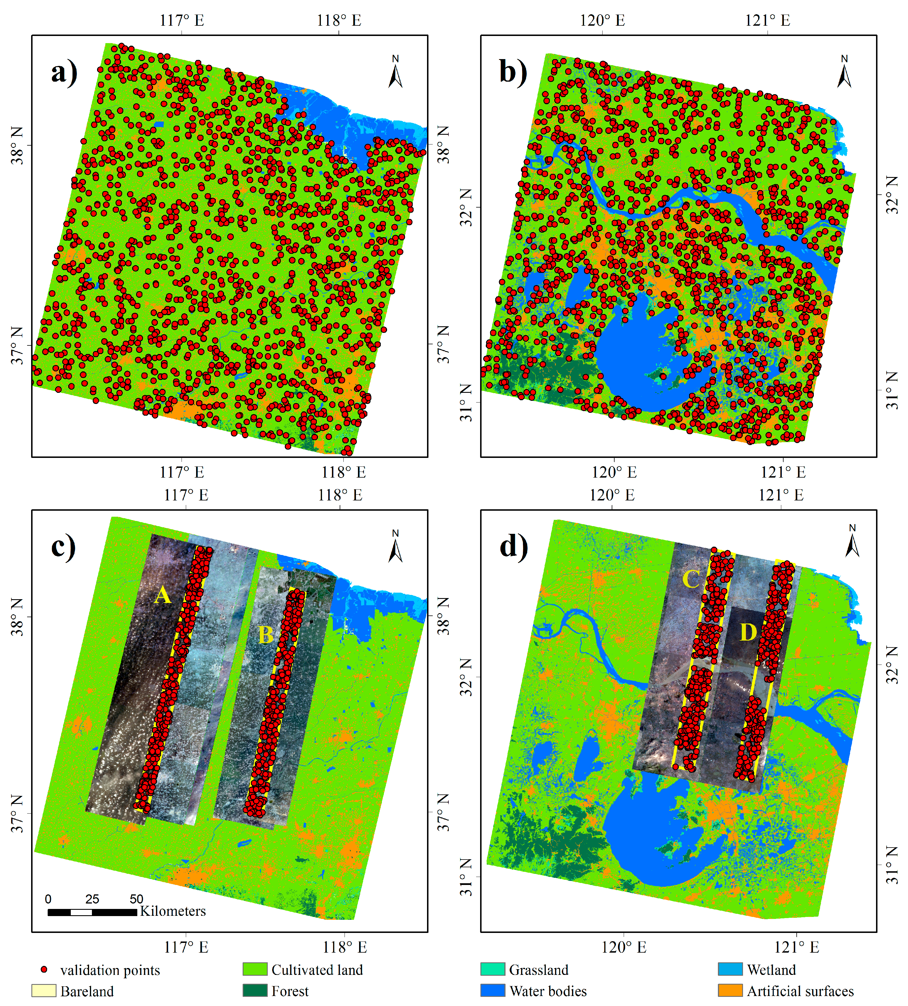
The cropping intensity maps for the study areas were assessed at two spatial scales: (1) the prefectural level; and (2) the pixel level. At the prefectural level, the gross sown areas derived from both the fusion and MODIS time series in 2015 were compared with that derived from national survey data from the 2016 provincial statistical yearbook, in which the official statistical data are released for the previous year. The gross sown areas for prefectures in SD and JS were obtained from Shandong Statistical Yearbook for 2016 [53] and Jiangsu Statistical Yearbook for 2016 [54]. At the pixel level, the cropping intensity maps were evaluated with 3000 sample points of croplands, where each scene contains 1500 sample points (Figure 5a,b). The sample points were randomly selected based on a stratified random sampling method, where 500 samples come from each of the three strata: fallow, single cropping, and double cropping. Professionals, without knowing the mapping results, visually interpreted the 3000 validation points based on the unfitted EVI time series at 30 m resolution. In addition, 1200 randomly selected sample points (i.e., 600 sample points for each scene and 200 sample points for the strata of fallow, single cropping, and double cropping, respectively) that distribute the overlapped areas of multi-temporal GF-1 and GF-2 images were interpreted based on the multi-temporal very high-resolution images of GF-1 and GF-2 for algorithm assessments (Figure 5c,d). The pixel was interpreted as double cropping if planted in both the spring season and the summer season and was interpreted as single cropping if planted only in the spring or the summer season.
4. Results
4.1. Mapping Results Using the Fusion Method of STARFM
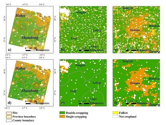
The mapped cropping cycles in 2015 for the two study scenes in both SD and JS are shown in Figure 6 and Figure 7, respectively. The spatial distribution of the cropping cycles is consistent with our general knowledge of cropping activities. For the SD scene, cropping intensities vary from double cropping to single cropping as the latitude increases, mostly because the climate and environment resource gradually become unsuitable for double cropping in northern Shandong Province in the North China Plain. For the JS scene, cropping intensities change from double cropping to single cropping as latitude decreases. The areas in southern Jiangsu Province in the Yangtze Downstream Plain experience fast economic development and urbanization, resulting in fragmental agricultural fields. Although the climate allows for planting multiple crops in a year, some farmers lived near the city area choose to plant crops only once a year or even leave the cropland uncultivated, because cultivating the croplands often costs higher capital and labor inputs but generates less net profits than working in the industry.
The spatial distributions of cropping cycles over the entire scenes are shown to be consistent as derived from the 30 m fusion data and the 500 m MODIS data. When inspecting the spatial pattern using the zoomed window, the mapped cropping cycles derived using the same method but from different datasets have obvious differences. The 500 m results could not depict the detail of land use as well as the 30 m results. For the SD scene, one zoomed image is located in a typical wheat-maize cultivated region with intensive double-cropping activities, and the other is located in a transition zone from single to double cropping. The 500 m results largely aggregate the agricultural lands and impervious areas, whereas the 30 m results show the field boundaries and shapes well and reduce the impacts of pixel mixture on mapping cropping cycles. Similarly, for the JS scenes, one zoomed image comes from the northern Jiangsu Province, where are cultivated with typical wheat-maize rotations, and another image covers an area mixed with wheat-rice and single rice cultivations. The 500 m results seem to erroneously depict the cropping activities near ponds and omit the spatial details of country roads and small towns, possibly because the pixels mixed with cropland and water at 500 m resolution could have time series of vegetation indices distinctively different from pixels of typical croplands.
At the prefectural level, the mapped cropping cycles are evaluated using the national census data reported by National Bureau of Statistics of China (NBSC) (Figure 8). To derive the sown areas from satellite-based maps, the cropland pixels are first multiplied by the cropping cycles and then zoned using the prefectural boundaries. The obtained coefficients of determination (R2) between satellite-derived and census-based sown areas are higher than 0.80 for both scene and for both the 30 m and 500 m maps, demonstrating that the developed method to derive cropping cycles performs reasonably well in both areas with regular field sizes like SD and areas with fragmental field sizes like JS. The algorithm shows to be robust when applied to satellite data at different spatial resolution and varied cultivated conditions. Note that the regression slopes between satellite-derived and census-based sown areas are much closer to the 1:1 line for the 30 m maps than for the 500 m maps for each scene. One possible reason is that the 30 m fusion data provide a realistic basis for estimating cropping areas because the pixel mixture effects are considerable at 500 m resolution and make it difficult to map agricultural fields accurately. For example, the regression slopes in the JS scene are higher than that in SD, probably due to more fragmental fields.
At the pixel scale, the 30 m cropping intensity maps derived from the 30 m time series data were evaluated using samples that were manually interpreted. The error matrices including the metrics of producer’s accuracy, user’s accuracy, overall accuracy are shown for each cropping classes and for each scene in Table 2. The achieved overall accuracies are 92.5% and 89.2% for the agricultural intensity map in the SD and JS scene, respectively, illustrating that the mapping results are accurate. The producer’s and user’s accuracies are all above 80.0% for three different classes of cropping activities. Most of commission errors are due to the confusion between single and double cropping, mainly because cloudy observations could result in missed data in the time series and make pixels of double cropping have time series data similar to pixels of single cropping. Other errors are resulted by the confusion between fallow and single cropping, largely due to the effects of pixel mixtures given that pixels mixed with single-cropping and fallow could have lower EVI than pure pixels with single cropping. The accuracies are generally higher in the SD scene than in the JS scene, because SD has fewer clouds and larger field sizes than JS.
The agriculture intensity maps at 30 m resolution were additionally evaluated using the samples derived from multi-temporal very high-resolution GF satellite images (Table 3). The overall accuracy is 81.2% for samples from four study regions and the overall accuracies are 82.0%, 82.3%, 81.3% and 79.0% for the Region A, B, C and D, respectively. The overall accuracies as evaluated using samples derived from multi-temporal GF-1 and GF-2 images are lower than those evaluated using samples derived from EVI time series. Similar to results in Table 2, the overall accuracies are slightly higher in SD than that of JS generally. In both regions A and B in SD, large errors are caused by the confusion between single cropping and fallow. By comparison, in both regions C and D in JS, large errors are due to the confusion between single cropping and double cropping.
To understand the scale effects on different resolution maps, the 30 m maps are aggregated to 500 m resolution as fractional maps of cropping intensities and are then compared with the binary 500 m map of cropping cycles. Each box diagram in the boxplots of Figure 9 shows the data distribution of fractional cropping intensities for each binary category of the cropping cycles. For the box diagram of fallow cycles derived using MODIS data, the mean marks of fractional cropping intensities are both less than 0.5, implying that using MODIS data alone might not be able to identify the cropping cycles accurately if the areas of cultivated lands occupy less than 50 percent of the pixels. The fusion data could be useful for identifying the cropping cycles for areas with small field sizes. By comparison, the box diagrams of double-cropping cycles derived using MODIS data in both SD and JS have the mean marks of fractional cropping intensities less than 2.0. In essence, because the effects of pixel mixture are considerable at 500 m resolution, applying the proposed method to the MODIS data at 500 m resolution tends to result in overestimates of double cropping and underestimates of fallow for areas with intensive agriculture. These results illustrate the necessaries to map cropping cycles at fine spatial resolutions.
4.2. Comparisons between Mapping Results Using STARFM and Using ESTARFM
The fusion methods determine the derived 30 m resolution surface reflectance data and hence the mapping results. While STARFM is implemented for producing high-resolution maps of cropping cycles, the algorithm of ESTARFM that uses two pairs of Landsat and MODIS images is another fusion method that has been widely used for data fusion. To understand the impacts of different fusion methods, we also implement ESTARFM [32] for data fusion. The real Landsat images are compared with fused images in Figure 10 and the results show that ESTARFM outperforms STARFM for the studied region in terms of the regression coefficients and error metrics. The linear correlations however are weaker than those in similar studies [31,32]. Note that we used 8-day composited products in our studies and there are two-day mismatches between MODIS composites and Landsat data. As the view angles could vary greatly in MODIS data from day to day, the fusion results are acceptable for subsequent analysis because noises in individual images could be reduced during the process of time series fitting.
The accuracies obtained using ESTARFM (Table 4) are comparable to those obtained using STARFM (Table 2) when assessing the mapping results using the interpreted samples. It appears that ESTARFM outperforms STARFM in recognition of single-cropping but underperforms STARFM for both fallow and double cropping possibly because that the fused images derived from ESTARFM have higher EVI values than those derived from STARFM. Comprehensive comparisons are needed in future studies to fully understand how different fusion approaches would influence their abilities on mapping cropping cycles using the proposed method. Note that STARFM requires only one pair of Landsat and MODIS images while ESTARFM requires two pairs of Landsat and MODIS images for data fusion and ESTARFM is much more computationally extensive than STARFM. Given that complete cloudy-free Landsat images during the growing season are not always available for other places and it is also quite possible that the matching MODIS images contain cloudy pixels, STARFM seems to be the method more suitable for large-scale applications.
5. Discussion
5.1. The Influence of the Field Sizes
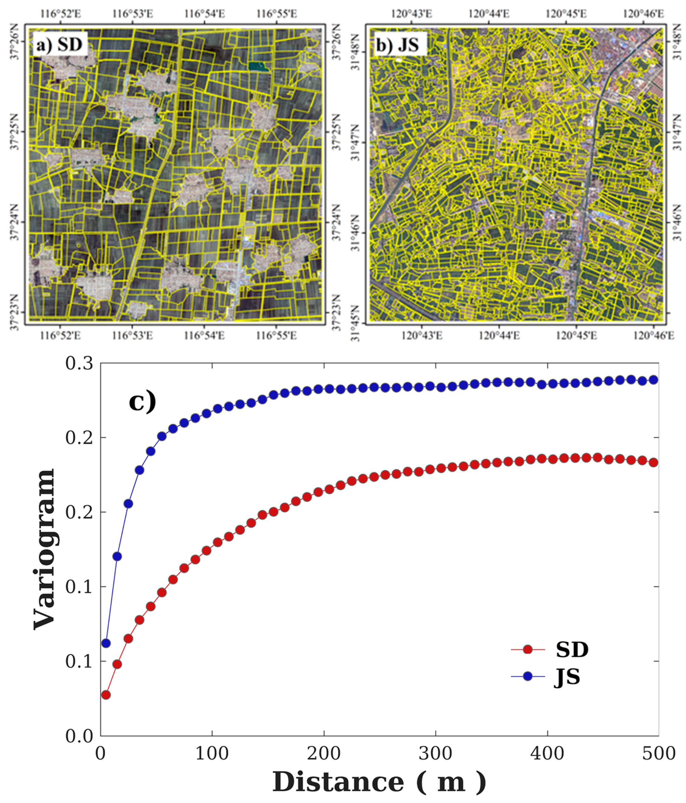
As the field sizes of the croplands could largely influence the mapping results [19], one key issue is to understand the needed spatial resolutions for mapping cropping cycles using remote sensing data. Figure 11 shows the hand-digitized GF-1 images that cover typical sites in both SD and JS (Figure 11a,b) and their corresponding variograms (Figure 11c) [55]. For the JS site (the dark blue line), the variogram rises steeply at small lag distances, indicating a large amount of small cropland fields. For the SD site (the dark red line), the variogram rises more slowly due to the presence of large crop fields. The variogram appears to reach its sill in the 100 to 200 m range for the JS site and in the 200 to 300 m range for the SD site, suggesting that the 500 m resolution of MODIS data is not sufficient for accurate mapping of cropping cycles in both SD and JS. The agricultural fields as quantified here are slightly larger than that in studies on Anhui Province of China [19] and all suggest that high-resolution mapping of agricultural lands and cropping cycles is needed for areas with fragmental croplands in China.
Mapping cropping cycles at fine resolution using time series satellite data generated by fusion of Landsat and MODIS has advantages over methods that use data from single satellite sensor. First, our results have shown that mapping cropping cycles at 30 m resolution provides more detailed distribution than at 500 m resolution for agricultural lands, and is more suitable for dealing with the effects of pixel mixtures. Second, the fusion approach solves the problem of lacking dense time series of satellite observations at fine resolution for tracking cropping activities on the ground.
5.2. Temporal Resolution of Satellite Data
In this work, we have implemented the fusion approach using 8-day composite MODIS data from both MOD09A1 and MYD09A1. The example for the time series of double cropping cycles (the black line) in Figure 4 suggests that 16-day composite MODIS products (e.g., MOD/MYD13Q1 EVI datasets) is likely unsuitable to be used for detecting cropping cycles because the temporal window between the harvest of the first crop and the plantation of the second crop is only 3–6 weeks. As a result, single points in the 16-day composite products missed during the key phenophases would lead to algorithm failures. By comparison, the uses of 8-day composite data allows for tracking the cropping activities using a predefined window. However, the cropping activities vary considerably over large geographic region, for example, the transplantation of the paddy rice frequently occurs in the southern China and crop maturation only requires a short growing time period, making it critical to obtain cloudy-free observations during the time period of crop rotation. It then would be of interests to test the fusion approach using daily MODIS data and produce daily time series for subsequent processing. Enriched high-resolution land surface observations from satellites like Landsat 8 and Sentinel 2 would allow for improving the mapping of cropping cycles, and how to minimize the differences among sensors and construct time series data at high spatial resolution with sufficient temporal resolution (less than or equal to 8-day) remains to be studied in future researches.
5.3. Cropland Mask
To screen out the croplands, we applied the land cover dataset of GlobeLand30 [38]. While the cropland mask in GlobeLand30 has shown to be sufficiently accurate in our experiments, we occasionally found that the impervious surfaces such as the roads in between villages and the ridges of crop field are not correctly classified but visible in our maps of cropping cycles. Given that the mapped cropping cycles in 2015 are five years later than the produced GlobeLand30 map 2010, it is necessary to understand how accurate the GlobeLand30 map is, and therefore we obtained ground survey data of polygons for the SD scene from National Bureau of Statistics of China. The polygon data were converted to raster data with binary classes of cropland and not cropland, which were used to evaluate the cropland mask derived from the GlobeLand30 map. The error matrix in Table 5 suggested an overall accuracy of 82.3% for the GlobeLand30 cropland mask. It is worth noting that the producer’s accuracy is 99.0% for the class of cropland but is only 20.5% for the class of not cropland, suggesting that many pixels that were not cropland are misclassified as cropland. Most of these erroneous classified areas were found to be mixed pixels in our examination. The confusion between impervious surfaces and agricultural lands could result in biased estimates of cropland areas and hence derived sown areas [17]. Improved mapping of croplands at high resolutions in future studies would help mapping of the cropping cycles as well [56].
6. Conclusions
While efforts have been made to map cropping intensities using satellite data, most of the approaches to date only tried to map cropping intensity at 500 m or even coarser resolution. In this study, we proposed a framework to identify cropping cycles at 30 m resolution by fusion of Landsat and MODIS. The method is tested in two typical regions of multiple cropping in major grain producing provinces in China. The mapping results were assessed at both the pixel and the county level. The overall accuracies are 92.5% and 89.2% for two study areas at the pixel level, respectively, and the R2 between satellite-derived and census-based sown areas are greater than 0.80. The distribution maps of cropping cycles at 30 m shows to depict the details of the agricultural field sizes better than the maps at 500 m resolution. The proposed method provides a potential way to map cropping intensities over large areas.
Acknowledgments
We thank anonymous reviewers for their constructive comments. This research is supported by National Key R&D Program of China (Grant Nos. 2017YFA0604302 and 2017YFA0604402), the Major Project of the University-Industry-Institute Collaboration Foundation of Guangzhou (Grant No. 156100021), and the Project of the Science and Technology Foundation of Guangdong Province (Grant No. 2015A010103013).
Author Contributions
Le Li designed the research and wrote the paper; Yaolong Zhao, Yingchun Fu, Yaozhong Pan, and Le Yu contributed to the interpretations; Yaozhong Pan contributed to the study datasets; and Qinchuan Xin performed data analysis and wrote the paper. All authors commented on and approved the final manuscript.
Conflicts of Interest
The authors declare no conflict of interest.
References
- FAO. Faostat Database on Agriculture. 2013. Available online: http://faostat.fao.org/ (accessed on 1 November 2017).
- Frolking, S.; Qiu, J.; Boles, S.; Xiao, X.; Liu, J.; Zhuang, Y.; Li, C.; Qin, X. Combining remote sensing and ground census data to develop new maps of the distribution of rice agriculture in China. Glob. Biogeochem. Cycles 2002, 16. [Google Scholar] [CrossRef]
- Gray, J.; Friedl, M.A.; Frolking, S.; Ramankutty, N.; Nelson, A.; Gumma, M.K. Mapping Asian Cropping Intensity With MODIS. IEEE J. Sel. Top. Appl. Earth Obs. Remote Sens. 2014, 7, 3373–3379. [Google Scholar] [CrossRef]
- Zhang, G.; Xiao, X.; Dong, J.; Kou, W.; Jin, C.; Qin, Y.; Zhou, Y.; Wang, J.; Menarguez, M.A.; Biradar, C. Mapping paddy rice planting areas through time series analysis of MODIS land surface temperature and vegetation index data. ISPRS J. Photogramm. Remote Sens. 2015, 106, 157–171. [Google Scholar] [CrossRef] [PubMed]
- Frolking, S.; Yeluripati, J.B.; Douglas, E.M. New district-level maps of rice cropping in India: A foundation for scientific input into policy assessment. Field Crop. Res. 2006, 98, 164–177. [Google Scholar] [CrossRef]
- Jain, M.; Mondal, P.; Defries, R.S.; Small, C.; Galford, G.L. Mapping cropping intensity of smallholder farms: A comparison of methods using multiple sensors. Remote Sens. Environ. 2013, 134, 210–223. [Google Scholar] [CrossRef]
- Gray, J.; Frolking, S.; Kort, E.A.; Ray, D.K.; Kucharik, C.J.; Ramankutty, N.; Friedl, M.A. Direct human influence on atmospheric CO2 seasonality from increased cropland productivity. Nature 2014, 515, 398–401. [Google Scholar] [CrossRef] [PubMed]
- Li, C.; Frolking, S.; Xiao, X.; Moore, B.; Boles, S.; Qiu, J.; Huang, Y.; Salas, W.; Sass, R.L. Modeling impacts of farming management alternatives on CO2, CH4, and N2O emissions: A case study for water management of rice agriculture of China. Glob. Biogeochem. Cycles 2005, 19. [Google Scholar] [CrossRef]
- Pittman, K.; Hansen, M.C.; Beckerreshef, I.; Potapov, P.; Justice, C.O. Estimating global cropland extent with multi-year MODIS data. Remote Sens. 2010, 2, 1844–1863. [Google Scholar] [CrossRef]
- Zhang, G.; Xiao, X.; Biradar, C.; Dong, J.; Qin, Y.; Menarguez, M.A.; Zhou, Y.; Zhang, Y.; Jin, C.; Wang, J. Spatiotemporal patterns of paddy rice croplands in China and India from 2000 to 2015. Sci. Total Environ. 2017, 579, 82–92. [Google Scholar] [CrossRef] [PubMed]
- Zhao, Y.; Bai, L.; Feng, J.; Lin, X.; Wang, L.; Xu, L.; Ran, Q.; Wang, K. Spatial and Temporal Distribution of Multiple Cropping Indices in the North China Plain Using a Long Remote Sensing Data Time Series. Sensors 2016, 16, 557. [Google Scholar] [CrossRef] [PubMed]
- Qiu, B.; Zhong, M.; Tang, Z.; Wang, C. A new methodology to map double-cropping croplands based on continuous wavelet transform. Int. J. Appl. Earth Obs. Geoinf. 2014, 26, 97–104. [Google Scholar] [CrossRef]
- Yan, H.; Xiao, X.; Huang, H.; Liu, J.; Chen, J.; Bai, X. Multiple cropping intensity in China derived from agro-meteorological observations and MODIS data. Chin. Geogr. Sci. 2014, 24, 205–219. [Google Scholar] [CrossRef]
- Liu, J.; Zhu, W.; Cui, X. A Shape-matching Cropping Index (CI) Mapping Method to Determine Agricultural Cropland Intensities in China using MODIS Time-series Data. Photogramm. Eng. Remote Sens. 2012, 78, 829–837. [Google Scholar] [CrossRef]
- Yan, H.; Liu, J.; Cao, M. Remotely sensed multiple cropping index variation during 1981–2000. ACTA Geogr. Sin. 2005, 60, 556–559. [Google Scholar]
- Ding, M.; Chen, Q.; Xiao, X.; Xin, L.; Zhang, G.; Li, L. Variation in Cropping Intensity in Northern China from 1982 to 2012 Based on GIMMS-NDVI Data. Sustainability 2016, 8, 1123. [Google Scholar] [CrossRef]
- Li, L.; Friedl, M.A.; Xin, Q.; Gray, J.; Pan, Y.; Frolking, S. Mapping Crop Cycles in China Using MODIS-EVI Time Series. Remote Sens. 2014, 6, 2473–2493. [Google Scholar] [CrossRef]
- Estel, S.; Kuemmerle, T.; Levers, C.; Baumann, M.; Hostert, P. Mapping cropland-use intensity across Europe using MODIS NDVI time series. Environ. Res. Lett. 2016, 11, 024015. [Google Scholar] [CrossRef]
- Ozdogan, M.; Woodcock, C.E. Resolution dependent errors in remote sensing of cultivated areas. Remote Sens. Environ. 2006, 103, 203–217. [Google Scholar] [CrossRef]
- Pan, Y.; Li, L.H.; Zhang, J.; Liang, S.; Zhu, X.; Sullamenashe, D. Winter wheat area estimation from MODIS-EVI time series data using the Crop Proportion Phenology Index. Remote Sens. Environ. 2012, 119, 232–242. [Google Scholar] [CrossRef]
- Shi, J.; Huang, J. Monitoring Spatio-Temporal Distribution of Rice Planting Area in the Yangtze River Delta Region Using MODIS Images. Remote Sens. 2015, 7, 8883–8905. [Google Scholar] [CrossRef]
- Pan, Y.; Hu, T.; Zhu, X.; Zhang, J.; Wang, X. Mapping Cropland Distributions Using a Hard and Soft Classification Model. IEEE Trans. Geosci. Remote Sens. 2012, 50, 4301–4312. [Google Scholar] [CrossRef]
- Wang, J.; Huang, J.; Zhang, K.; Li, X.; She, B.; Wei, C.; Gao, J.; Song, X. Rice Fields Mapping in Fragmented Area Using Multi-Temporal HJ-1A/B CCD Images. Remote Sens. 2015, 7, 3467–3488. [Google Scholar] [CrossRef]
- Son, N.T.; Chen, C.; Chen, C.; Duc, H.; Chang, L. A Phenology-Based Classification of Time-Series MODIS Data for Rice Crop Monitoring in Mekong Delta, Vietnam. Remote Sens. 2013, 6, 135–156. [Google Scholar] [CrossRef]
- Xin, Q.; Olofsson, P.; Zhu, Z.; Tan, B.; Woodcock, C.E. Toward near real-time monitoring of forest disturbance by fusion of MODIS and Landsat data. Remote Sens. Environ. 2013, 135, 234–247. [Google Scholar] [CrossRef]
- Gevaert, C.M.; Garciaharo, F.J. A comparison of STARFM and an unmixing-based algorithm for Landsat and MODIS data fusion. Remote Sens. Environ. 2015, 156, 34–44. [Google Scholar] [CrossRef]
- Zhang, W.; Li, A.; Jin, H.; Bian, J.; Zhang, Z.; Lei, G.; Qin, Z.; Huang, C. An enhanced spatial and temporal data fusion model for fusing Landsat and MODIS surface reflectance to generate high temporal Landsat-like data. Remote Sens. 2013, 5, 5346–5368. [Google Scholar] [CrossRef]
- Walker, J.J.; De Beurs, K.M.; Wynne, R.H.; Gao, F. Evaluation of Landsat and MODIS data fusion products for analysis of dryland forest phenology. Remote Sens. Environ. 2012, 117, 381–393. [Google Scholar] [CrossRef]
- Jarihani, A.A.; Mcvicar, T.R.; Van Niel, T.G.; Emelyanova, I.; Callow, J.N.; Johansen, K. Blending Landsat and MODIS Data to Generate Multispectral Indices: A Comparison of “Index-then-Blend” and “Blend-then-Index” Approaches. Remote Sens. 2014, 6, 9213–9238. [Google Scholar] [CrossRef] [Green Version]
- Wu, M.; Zhang, X.; Huang, W.; Niu, Z.; Wang, C.; Li, W.; Hao, P. Reconstruction of Daily 30m Data from HJ CCD, GF-1 WFV, Landsat, and MODIS Data for Crop Monitoring. Remote Sens. 2015, 7, 16293–16314. [Google Scholar] [CrossRef]
- Gao, F.; Masek, J.G.; Schwaller, M.; Hall, F.G. On the blending of the Landsat and MODIS surface reflectance: Predicting daily Landsat surface reflectance. IEEE Trans. Geosci. Remote Sens. 2006, 44, 2207–2218. [Google Scholar]
- Zhu, X.; Chen, J.; Gao, F.; Chen, X.; Masek, J.G. An enhanced spatial and temporal adaptive reflectance fusion model for complex heterogeneous regions. Remote Sens. Environ. 2010, 114, 2610–2623. [Google Scholar] [CrossRef]
- Hilker, T.; Wulder, M.A.; Coops, N.C.; Linke, J.; Mcdermid, G.; Masek, J.G.; Gao, F.; White, J.C. A new data fusion model for high spatial- and temporal-resolution mapping of forest disturbance based on Landsat and MODIS. Remote Sens. Environ. 2009, 113, 1613–1627. [Google Scholar] [CrossRef]
- Wu, M.; Niu, Z.; Wang, C.; Wu, C.; Wang, L. Use of MODIS and Landsat time series data to generate high-resolution temporal synthetic Landsat data using a spatial and temporal reflectance fusion model. J. Appl. Remote Sens. 2012, 6. [Google Scholar] [CrossRef]
- Earth Resources Observation and Science (EROS) Center Science Processing Architecture (ESPA). Available online: https://espa.cr.usgs.gov/ (accessed on 1 November 2017).
- Land Processes Distributed Active Archive Center (LPDAAC). Available online: https://lpdaac.usgs.gov (accessed on 1 November 2017).
- National Geomatics Center of China. Available online: http://www.globeland30.org (accessed on 1 November 2017).
- Chen, J.; Chen, J.; Liao, A.; Cao, X.; Chen, L.; Chen, X.; He, C.; Han, G.; Peng, S.; Lu, M. Global land cover mapping at 30 m resolution: A POK-based operational approach. ISPRS J. Photogramm. Remote Sens. 2015, 103, 7–27. [Google Scholar] [CrossRef]
- China Center for Resources Satellite Data and Applications. Available online: www.cresda.com (accessed on 1 November 2017).
- Gumma, M.K.; Thenkabail, P.S.; Maunahan, A.; Islam, S.; Nelson, A. Mapping seasonal rice cropland extent and area in the high cropping intensity environment of Bangladesh using MODIS 500 m data for the year 2010. ISPRS J. Photogramm. Remote Sens. 2014, 91, 98–113. [Google Scholar] [CrossRef]
- Xiao, X.; Boles, S.; Frolking, S.; Li, C.; Babu, J.; Salas, W.; Moore, B. Mapping paddy rice agriculture in South and Southeast Asia using multi-temporal MODIS images. Remote Sens. Environ. 2006, 100, 95–113. [Google Scholar] [CrossRef]
- Bolton, D.K.; Friedl, M.A. Forecasting crop yield using remotely sensed vegetation indices and crop phenology metrics. Agric. For. Meteorol. 2013, 173, 74–84. [Google Scholar] [CrossRef]
- Huete, A.R.; Didan, K.; Miura, T.; Rodriguez, E.P.; Gao, X.; Ferreira, L.G. Overview of the radiometric and biophysical performance of the MODIS vegetation indices. Remote Sens. Environ. 2002, 83, 195–213. [Google Scholar] [CrossRef]
- Guindingarcia, N.; Gitelson, A.A.; Arkebauer, T.J.; Shanahan, J.F.; Weiss, A. An evaluation of MODIS 8- and 16-day composite products for monitoring maize green leaf area index. Agric. For. Meteorol. 2012, 161, 15–25. [Google Scholar] [CrossRef]
- Wardlow, B.D.; Egbert, S.L.; Kastens, J.H. Analysis of time-series MODIS 250 m vegetation index data for crop classification in the U.S. Central Great Plains. Remote Sens. Environ. 2007, 108, 290–310. [Google Scholar] [CrossRef]
- Lobell, D.B.; Asner, G.P. Cropland distributions from temporal unmixing of MODIS data. Remote Sens. Environ. 2004, 93, 412–422. [Google Scholar] [CrossRef]
- Xiao, X.; Boles, S.; Liu, J.; Zhuang, D.; Frolking, S.; Li, C.; Salas, W.; Moore, B. Mapping paddy rice agriculture in southern China using multi-temporal MODIS images. Remote Sens. Environ. 2005, 95, 480–492. [Google Scholar] [CrossRef]
- Sakamoto, T.; Van Nguyen, N.; Ohno, H.; Ishitsuka, N.; Yokozawa, M. Spatio-temporal distribution of rice phenology and cropping systems in the Mekong Delta with special reference to the seasonal water flow of the Mekong and Bassac rivers. Remote Sens. Environ. 2006, 100, 1–16. [Google Scholar] [CrossRef]
- Sakamoto, T.; Yokozawa, M.; Toritani, H.; Shibayama, M.; Ishitsuka, N.; Ohno, H. A crop phenology detection method using time-series MODIS data. Remote Sens. Environ. 2005, 96, 366–374. [Google Scholar] [CrossRef]
- Zhang, X.; Friedl, M.A.; Schaaf, C.B.; Strahler, A.H.; Hodges, J.C.F.; Gao, F.; Reed, B.C.; Huete, A.R. Monitoring vegetation phenology using MODIS. Remote Sens. Environ. 2003, 84, 471–475. [Google Scholar] [CrossRef]
- Dong, J.; Xiao, X.; Kou, W.; Qin, Y.; Zhang, G.; Li, L.; Jin, C.; Zhou, Y.; Wang, J.; Biradar, C. Tracking the dynamics of paddy rice planting area in 1986–2010 through time series Landsat images and phenology-based algorithms. Remote Sens. Environ. 2015, 160, 99–113. [Google Scholar] [CrossRef]
- Boschetti, M.R.; Stroppiana, D.; Brivio, P.A.; Bocchi, S. Multi-year monitoring of rice crop phenology through time series analysis of MODIS images. Int. J. Remote Sens. 2009, 30, 4643–4662. [Google Scholar] [CrossRef]
- Shandong Statistical Yearbook for 2016. Available online: http://www.stats-sd.gov.cn (accessed on 1 November 2017).
- Jiangsu Statistical Yearbook for 2016. Available online: http://www.jssb.gov.cn (accessed on 1 November 2017).
- Woodcock, C.E.; Strahler, A.H. The factor of scale in remote sensing. Remote Sens. Environ. 1987, 21, 311–332. [Google Scholar] [CrossRef]
- Yu, L.; Wang, J.; Clinton, N.; Xin, Q.; Zhong, L.; Chen, Y.; Gong, P. FROM-GC: 30 m global cropland extent derived through multisource data integration. Int. J. Digit. Earth 2013, 6, 521–533. [Google Scholar] [CrossRef]
Figure 1.
An overview of the study area is shown for the Landsat 8 images based on the false-color composites of near-infrared, red, and blue bands.
Figure 1.
An overview of the study area is shown for the Landsat 8 images based on the false-color composites of near-infrared, red, and blue bands.

Figure 2.
The flowchart for mapping cropping cycles.
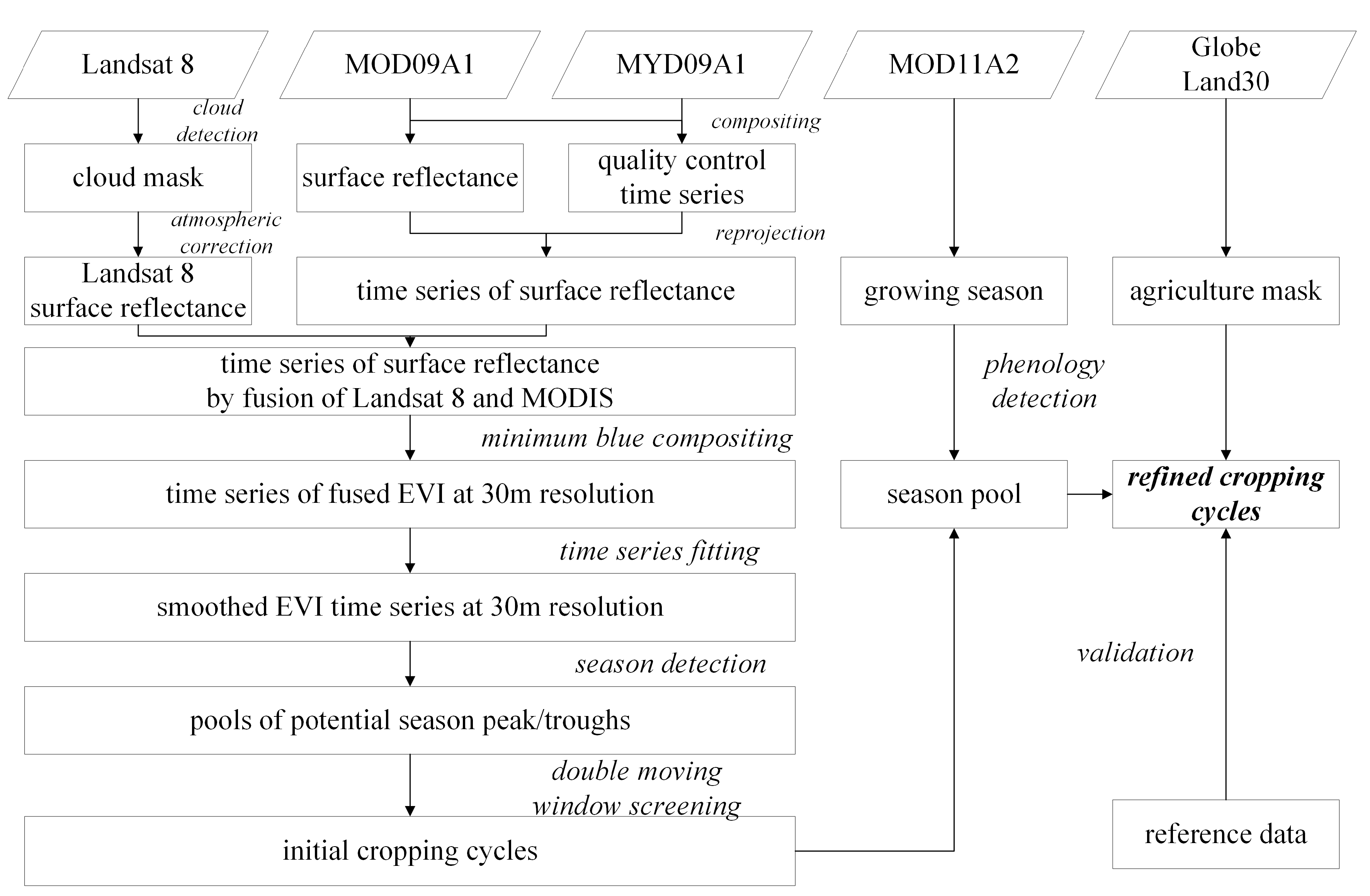
Figure 3.
Examples are shown for the surface reflectance images after fusion of Landsat and MODIS data and real Landsat data. The top line shows the fusion results for the entire SD scene, and the second line shows for a zoomed area as outlined by the yellow box, the third line shows for the real Landsat data, and the bottom line shows for the zoomed area as outlined by the yellow box. The images are shown for the false-color composite of near-infrared, red, and blue bands.

Figure 4.
Examples of the processes of EVI time series are shown for typical points of fallow, single cropping and double cropping in the Shandong scene. The fused EVI time series are composited from both MODIS Terra and Aqua data based on the minimum blue compositing method, and cloudy observations are identified based on the quality control data of original MODIS observations. The geographic coordinates for the fallow, single-cropping and double-cropping pixels are (38.082°N, 116.560°E), (37.604°N, 118.264°E), and (37.439°N, 116.866°E), respectively.
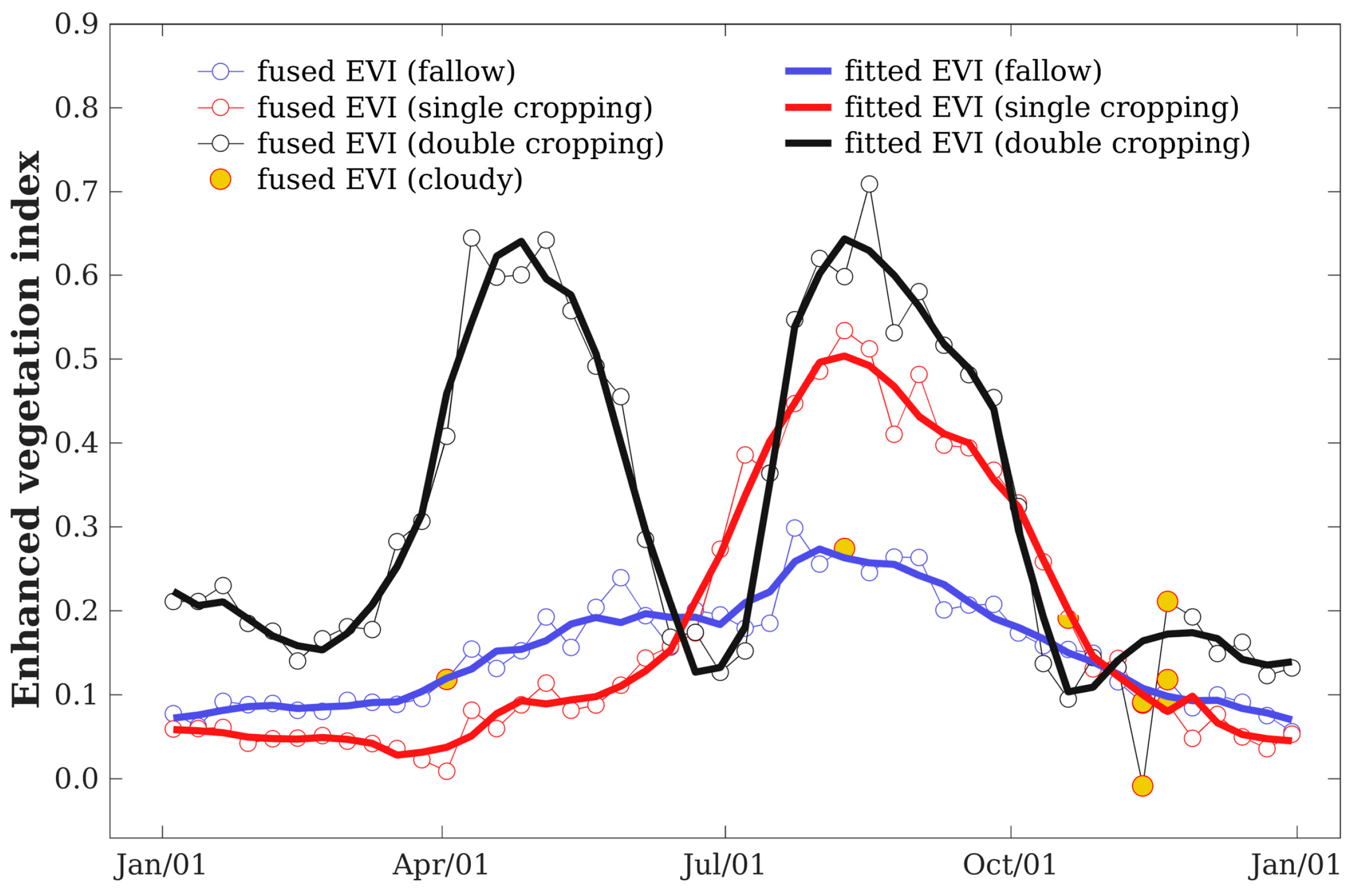
Figure 5.
Locations of validation points are shown for: (a) SD; and (b) JS, as derived from unfitted EVI time series data on the backdrop of the GlobeLand30 land cover maps; and (c) SD; and (d) JS, as derived from multi-temporal very high-resolution images of GF-1 and GF-2 on the backdrop of the GlobeLand30 land cover maps.

Figure 6.
Mapped cropping cycles for the SD scene and zoomed images. Images are shown for the distribution maps derived from the 30 m fusion data (top row, a–c) and from 500 m MODIS data (bottom row, d–f), respectively. The left column presents maps of cropping cycles for the entire scene, and the middle and the right column present two zoomed areas as marked by the red windows.

Figure 7.
Mapped cropping cycles for the JS scene and zoomed images. Images are shown for the distribution maps derived from the 30 m fusion data (top row, a–c) and from 500 m MODIS data (bottom row, d–f), respectively. The left column presents maps of cropping cycles for the entire scene, and the middle and the right column present two zoomed areas as marked by the red windows.

Figure 8.
Gross sown areas for the year of 2015 are compared between national census data at the county level and maps of cropping cycles as derived from: (a) SD; and (b) JS. The black dots represent estimates derived from 30 m fusion data and the blue hollow dots represent estimates derived from the 500 m MODIS data.
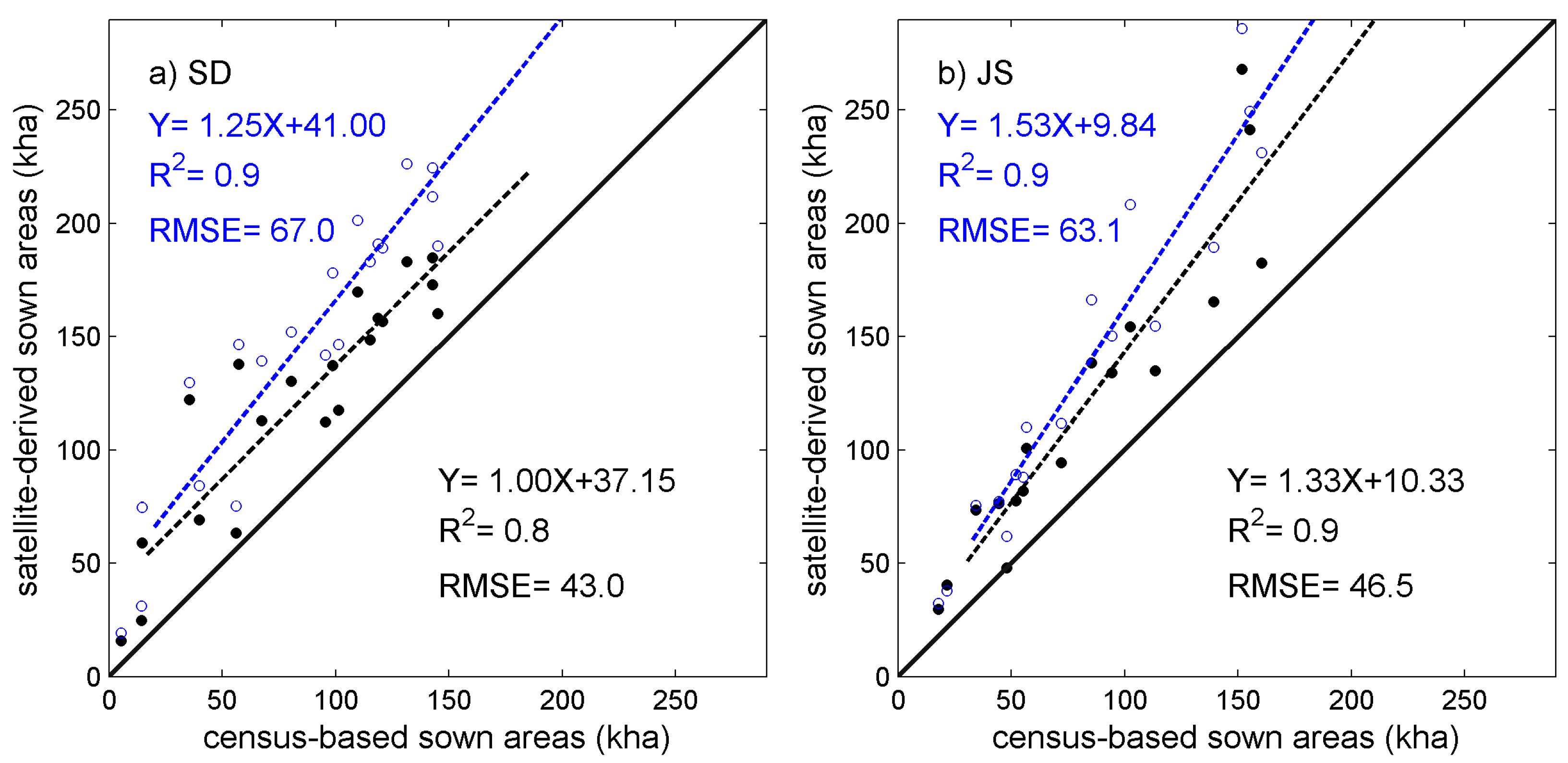
Figure 9.
The boxplots for the distribution of crop intensities are shown for the scenes of: (a) SD; and (b) JS. The 30 m cropping cycles mapped using the fusion data are aggregated to 500 m as fractional maps and are then compared with the binary cropping cycles mapped using the 500 m MODIS data for the entire scene.
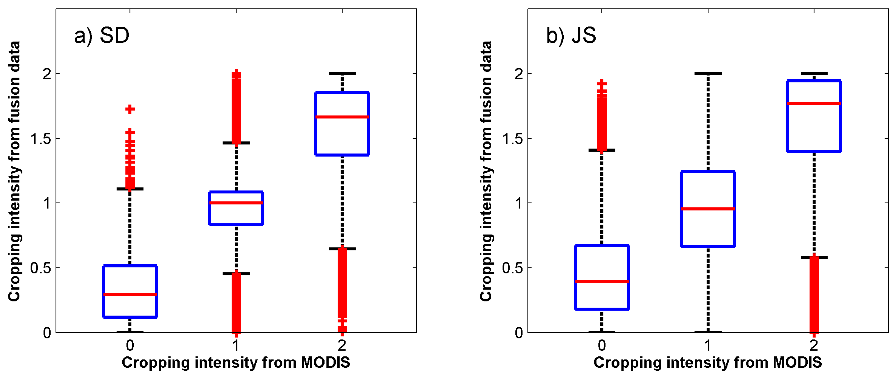
Figure 10.
Scatter plots of real surface reflectance and predicted surface reflectance in near-infrared and red bands using STARFM (a,b) and ESTARFM (c,d). The solid lines denote the 1:1 lines and the dash lines denote the regression lines.
Figure 10.
Scatter plots of real surface reflectance and predicted surface reflectance in near-infrared and red bands using STARFM (a,b) and ESTARFM (c,d). The solid lines denote the 1:1 lines and the dash lines denote the regression lines.
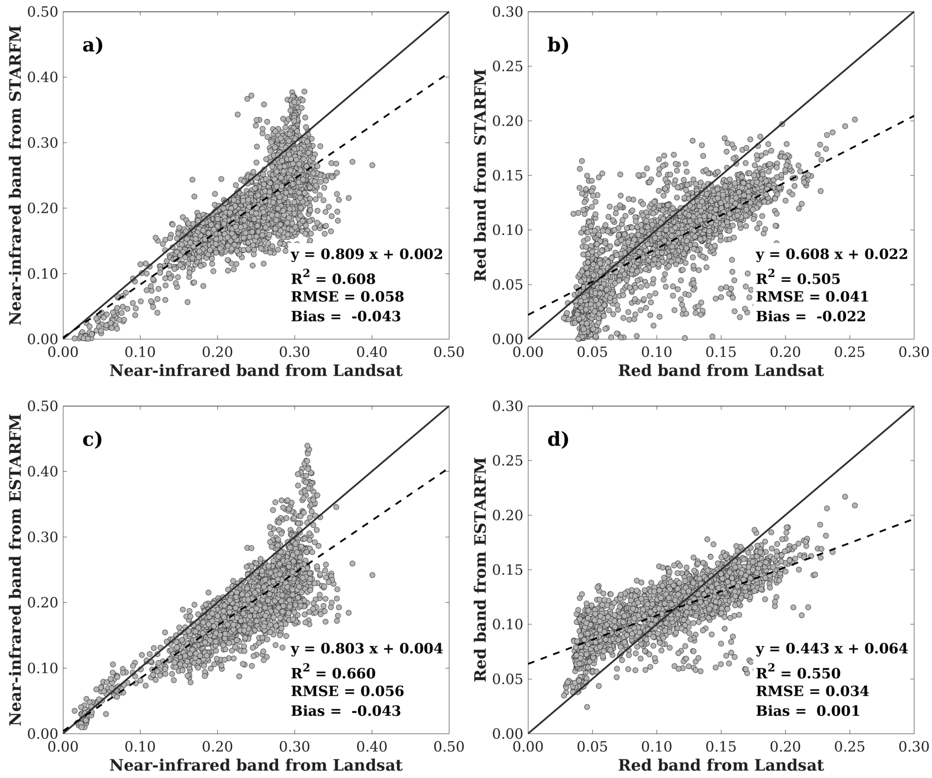
Figure 11.
The hand-digitized polygons on the backdrops of GF1 images in both: (a) SD; and (b) JS; and (c) the corresponding variogram.
Figure 11.
The hand-digitized polygons on the backdrops of GF1 images in both: (a) SD; and (b) JS; and (c) the corresponding variogram.

Table 1.
Information on all Landsat 8 images (cloud cover <10%) in 2015 for two studied scenes.
| Path, Row | Date | Scene Cloud Cover Percentage (%) | Land Cloud Cover Percentage (%) |
|---|---|---|---|
| 122, 034 | 19 January 2015 | 0.28 | 0.27 |
| 4 February 2015 | 9.14 | 9.03 | |
| 24 March 2015 | 0.81 | 0.79 | |
| 25 April 2015 | 1.86 | 1.81 | |
| 12 June 2015 | 1.59 | 0.84 | |
| 16 September 2015 | 1.54 | 1.54 | |
| 2 October 2015 | 0.09 | 0.09 | |
| 3 November 2015 | 0.72 | 0.70 | |
| 119, 038 | 27 September 2015 | 7.02 | 7.30 |
| 13 October 2015 | 3.20 | 3.29 | |
| 16 December 2015 | 6.60 | 6.71 |
Table 2.
The error matrices for the agricultural intensity maps in 2015 for both scenes using STARFM.
Table 2.
The error matrices for the agricultural intensity maps in 2015 for both scenes using STARFM.
| Mapped Classes | Reference Data | |||||||
|---|---|---|---|---|---|---|---|---|
| Shandong Scene | Jiangsu Scene | |||||||
| F | S | D | UA (%) | F | S | D | UA (%) | |
| F | 466 | 27 | 7 | 93.2% | 448 | 43 | 9 | 89.6% |
| S | 10 | 454 | 36 | 90.8% | 26 | 439 | 35 | 87.8% |
| D | 4 | 29 | 467 | 93.4% | 0 | 49 | 451 | 90.2% |
| PA (%) | 97.1% | 89.0% | 91.6% | 94.5% | 82.7% | 91.1% | ||
| OA (%) | 92.5% | 89.2% | ||||||
F denotes fallow; S denotes single-cropping; D denotes double-cropping; and PA, OA, and UA denote producer’s accuracy, overall accuracy and user’s accuracy, respectively.
Table 3.
The error matrices for the agricultural intensity maps using reference data derived from multi-temporal very high-resolution GF-1 and GF-2 images.
Table 3.
The error matrices for the agricultural intensity maps using reference data derived from multi-temporal very high-resolution GF-1 and GF-2 images.
| Mapped Classes | Reference for Region A | Reference for Region B | Reference for Region C | Reference for Region D | ||||||||||||
|---|---|---|---|---|---|---|---|---|---|---|---|---|---|---|---|---|
| F | S | D | UA (%) | F | S | D | UA (%) | F | S | D | UA (%) | F | S | D | UA (%) | |
| F | 84 | 11 | 5 | 84.0 | 86 | 11 | 3 | 86.0 | 87 | 11 | 2 | 87.0 | 76 | 18 | 6 | 76.0 |
| S | 5 | 77 | 18 | 77.0 | 10 | 78 | 12 | 78.0 | 13 | 76 | 11 | 76.0 | 11 | 71 | 18 | 71.0 |
| D | 1 | 14 | 85 | 85.0 | 3 | 14 | 83 | 83.0 | 8 | 11 | 81 | 81.0 | 3 | 7 | 90 | 90.0 |
| PA (%) | 93.3 | 75.5 | 78.7 | 86.9 | 75.7 | 84.7 | 80.6 | 77.6 | 86.2 | 84.4 | 74.0 | 78.9 | ||||
| OA (%) | 82.0 | 82.3 | 81.3 | 79.0 | ||||||||||||
| OA (%) for all samples: 81.2% | ||||||||||||||||
F denotes fallow; S denotes single-cropping; D denotes double-cropping; and PA, OA, and UA denote producer’s accuracy, overall accuracy and user’s accuracy, respectively.
Table 4.
The error matrices for the agricultural intensity maps in 2015 for both scenes using ESTARFM.
Table 4.
The error matrices for the agricultural intensity maps in 2015 for both scenes using ESTARFM.
| Mapped Classes | Reference Data | |||||||
|---|---|---|---|---|---|---|---|---|
| Shandong Scene | Jiangsu Scene | |||||||
| F | S | D | UA (%) | F | S | D | UA (%) | |
| F | 432 | 56 | 12 | 86.4% | 420 | 52 | 28 | 84.0% |
| S | 15 | 464 | 21 | 92.8% | 19 | 454 | 27 | 90.8% |
| D | 26 | 45 | 429 | 85.8% | 8 | 61 | 431 | 86.2% |
| PA(%) | 91.3% | 82.1% | 92.9% | 94.0% | 80.1% | 88.7% | ||
| OA(%) | 88.3% | 87.0% | ||||||
F denotes fallow; S denotes single-cropping; D denotes double-cropping; and PA, OA and UA denote producer’s accuracy, overall accuracy and user’s accuracy, respectively.
Table 5.
The error matrix for the GlobeLand30 map in SD as evaluated using ground survey data.
| GlobeLand30 Map | Ground Survey | ||
|---|---|---|---|
| Cropland | Not Cropland | User’s Accuracy | |
| Cropland | 129,940 | 28,073 | 82.2% |
| Not cropland | 1364 | 7258 | 84.2% |
| Producer’s accuracy | 99.0% | 20.5% | |
| Overall accuracy | 82.3% | ||
© 2017 by the authors. Licensee MDPI, Basel, Switzerland. This article is an open access article distributed under the terms and conditions of the Creative Commons Attribution (CC BY) license (http://creativecommons.org/licenses/by/4.0/).
Share and Cite
MDPI and ACS Style
Li, L.; Zhao, Y.; Fu, Y.; Pan, Y.; Yu, L.; Xin, Q. High Resolution Mapping of Cropping Cycles by Fusion of Landsat and MODIS Data. Remote Sens. 2017, 9, 1232. https://doi.org/10.3390/rs9121232
AMA Style
Li L, Zhao Y, Fu Y, Pan Y, Yu L, Xin Q. High Resolution Mapping of Cropping Cycles by Fusion of Landsat and MODIS Data. Remote Sensing. 2017; 9(12):1232. https://doi.org/10.3390/rs9121232
Chicago/Turabian StyleLi, Le, Yaolong Zhao, Yingchun Fu, Yaozhong Pan, Le Yu, and Qinchuan Xin. 2017. "High Resolution Mapping of Cropping Cycles by Fusion of Landsat and MODIS Data" Remote Sensing 9, no. 12: 1232. https://doi.org/10.3390/rs9121232
Note that from the first issue of 2016, this journal uses article numbers instead of page numbers. See further details here.