Normalized Difference Vegetation Index as an Estimator for Abundance and Quality of Avian Herbivore Forage in Arctic Alaska

Abstract
:
1. Introduction
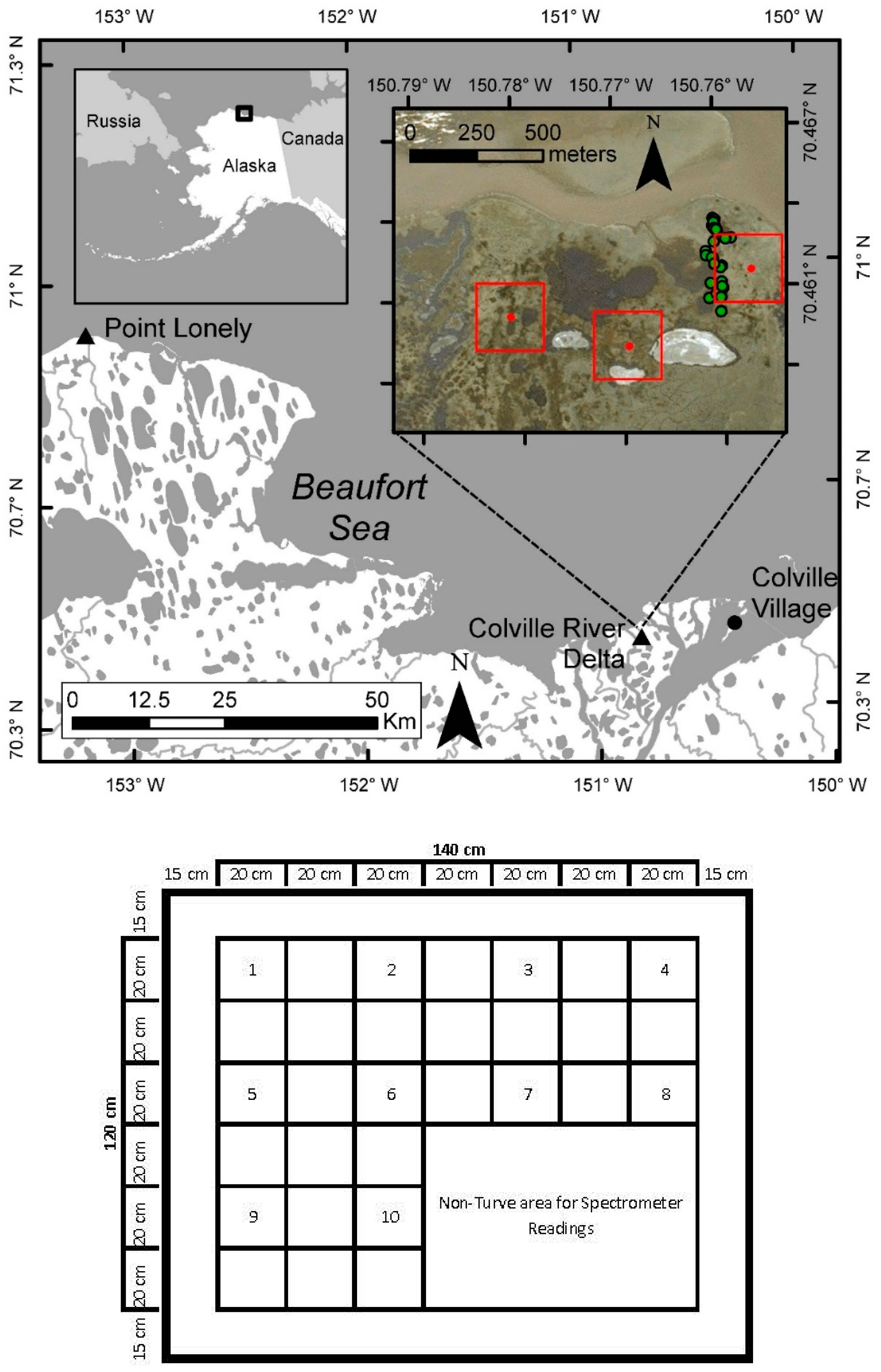
2. Study Area
3. Methods
3.1. Vegetation Sampling and Processing
3.2. Environmental Data
3.3. NDVI Data
3.4. Analyses
3.4.1. Predicting Aboveground Biomass and Nitrogen Biomass Using NDVI
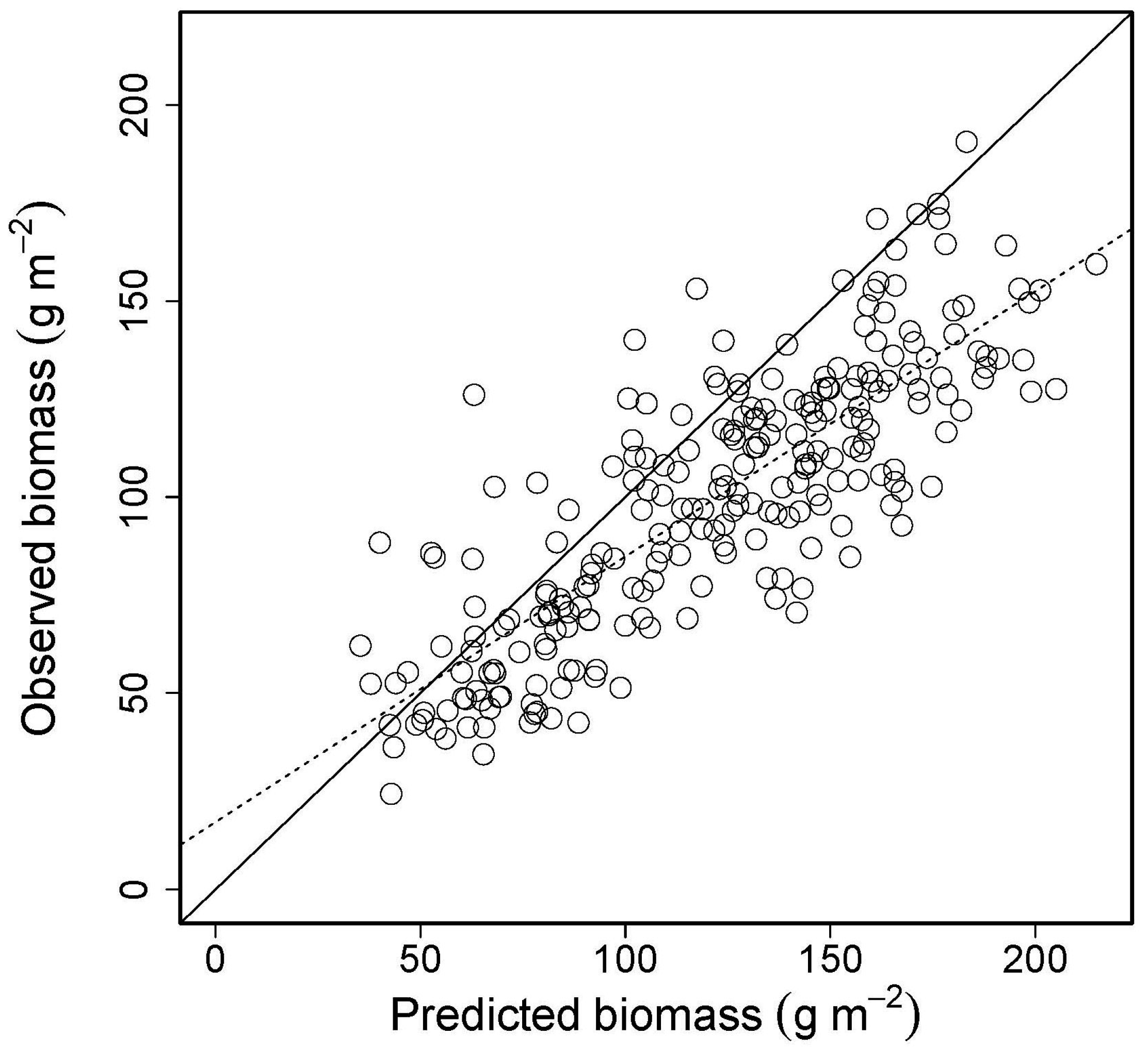
3.4.2. Validation: Prediction of Biomass
3.4.3. Phenology Metric: Linking Seasonal Phenology in NDVI and Percent Nitrogen
3.4.4. Phenology Curve Fitting and Metric Estimation
3.4.5. Assessing Predictive Power of Phenology Metrics
4. Results
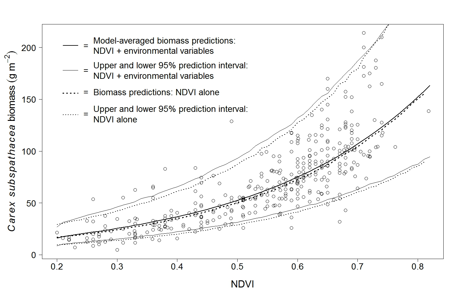
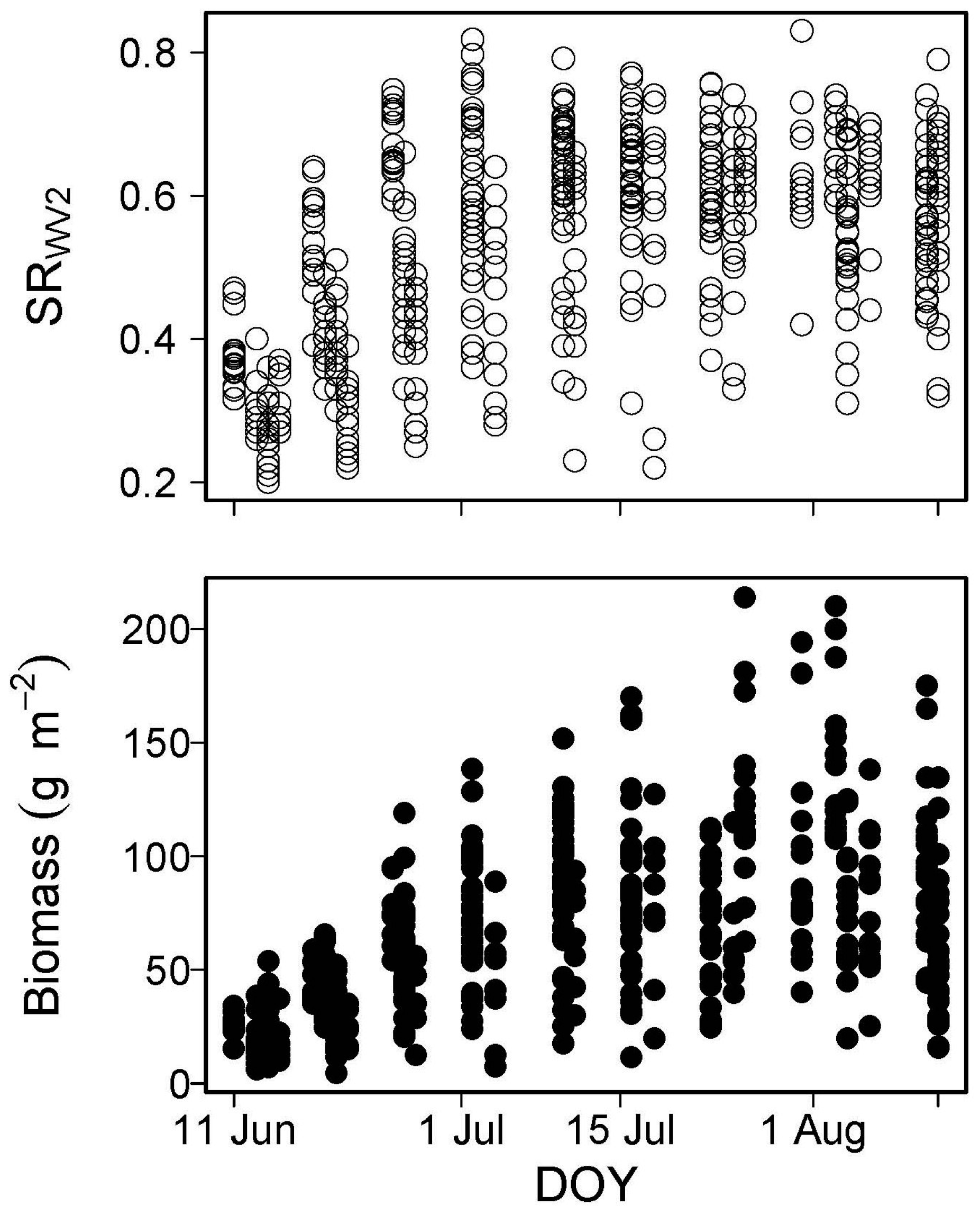
4.1. Predictions of Biomass and Nitrogen Biomass
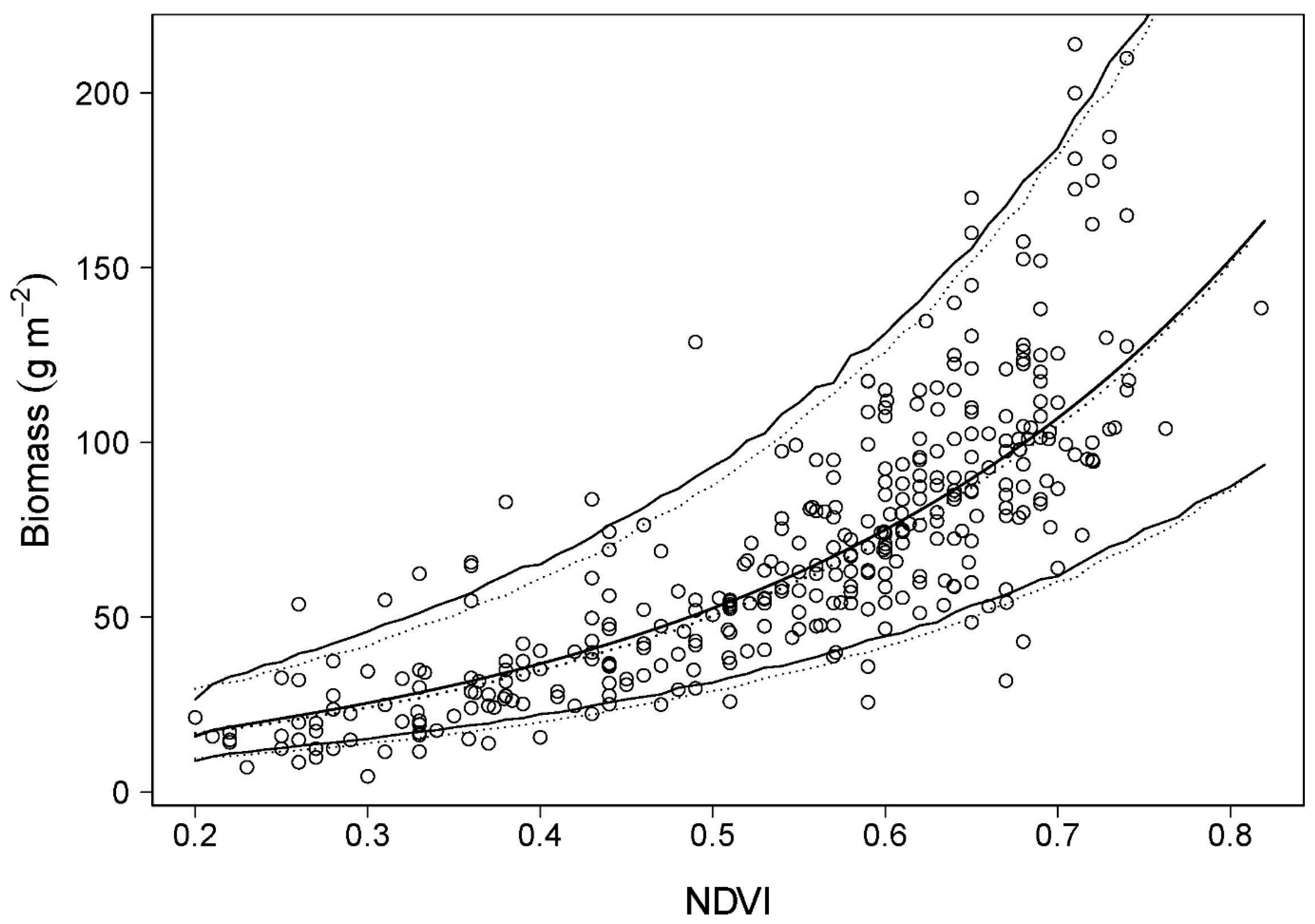
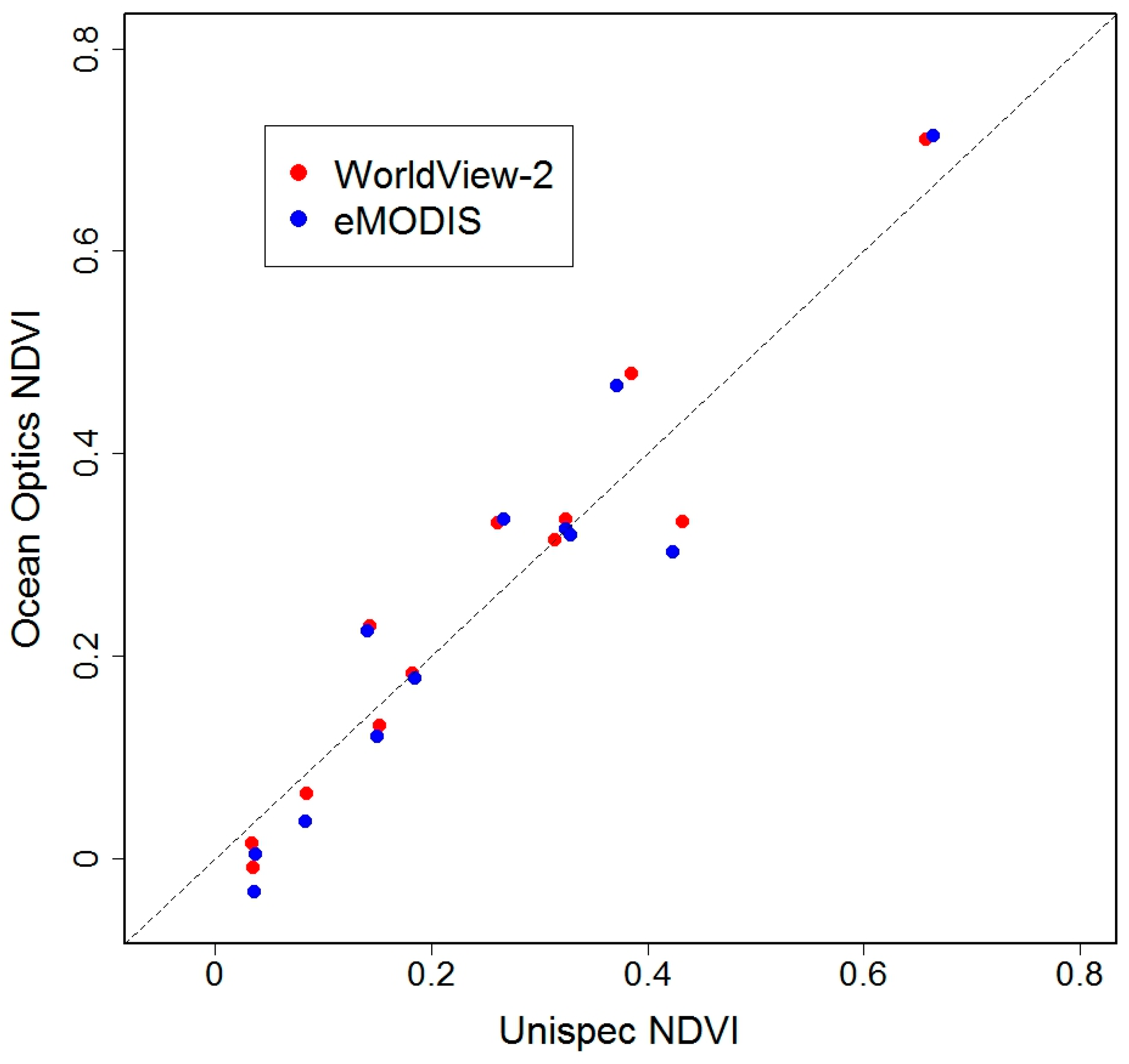
4.2. Validation: Estimation of Biomass at PL Using Spectrometer-Derived NDVI
4.3. NDVI as a Phenology Metric
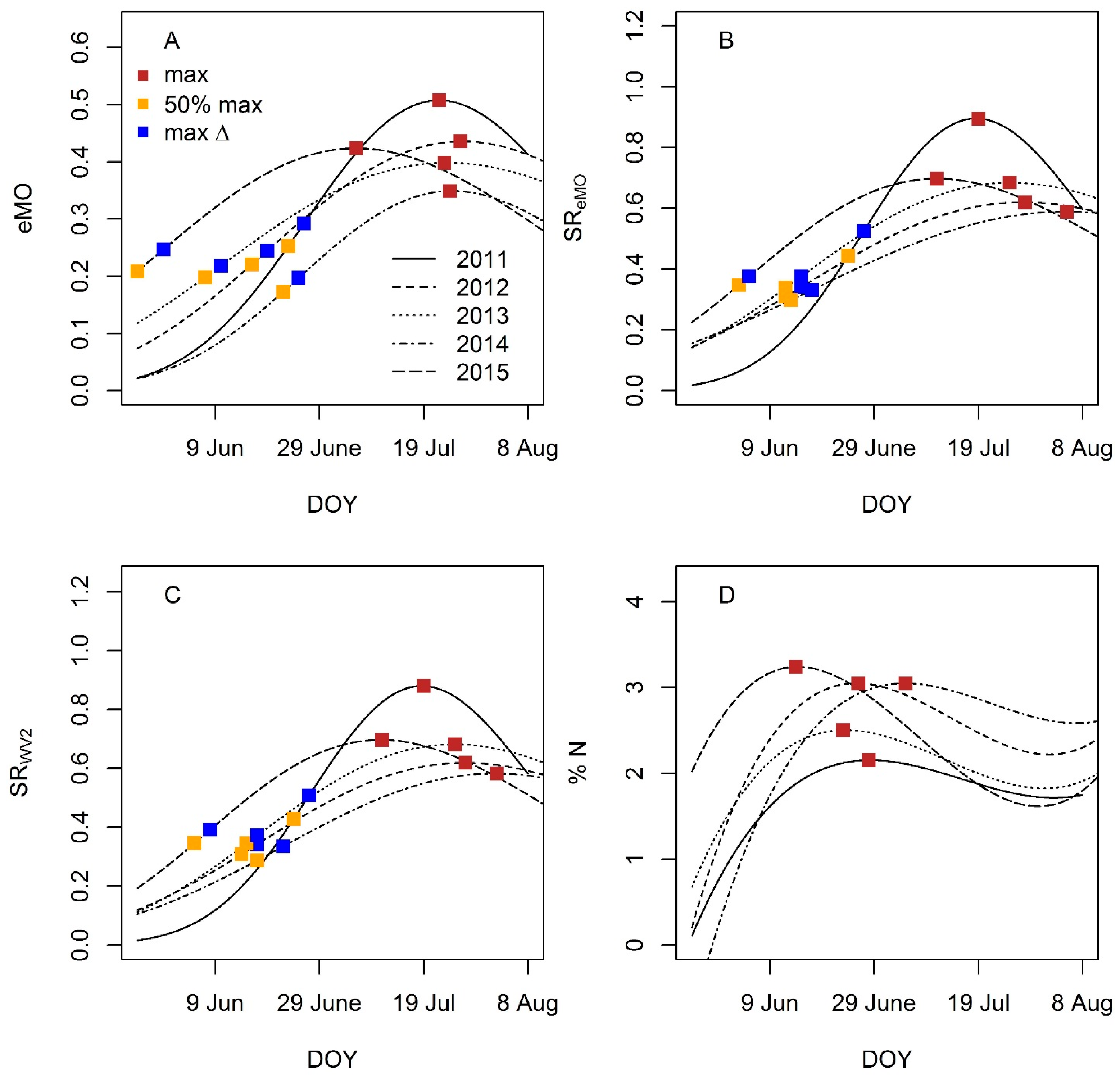
4.3.1. Seasonal Dynamics of NDVI and Percent Nitrogen
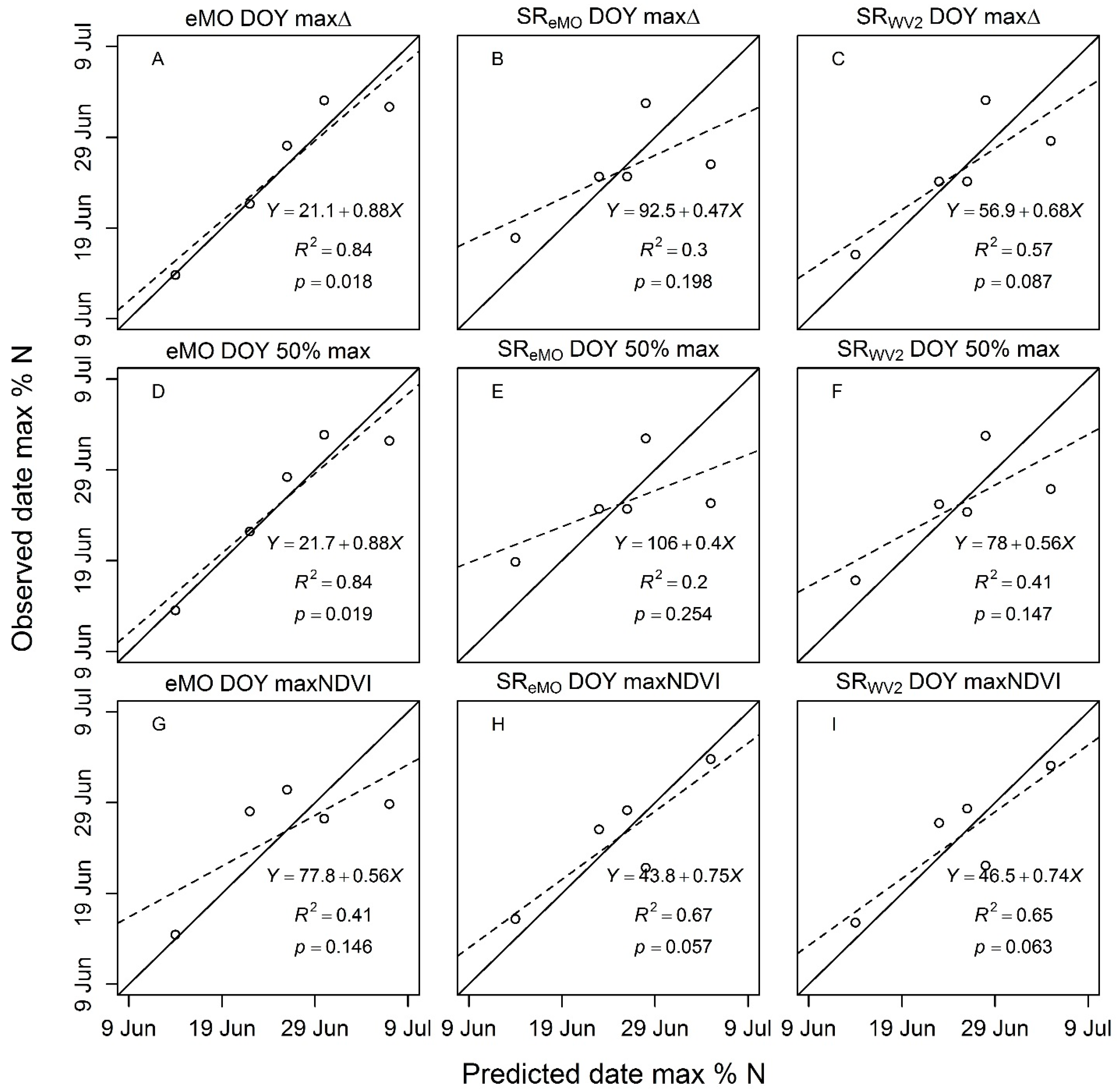
4.3.2. Phenology Metric Estimation and Performance
5. Discussion
5.1. NDVI as an Estimator of Biomass and Nitrogen
5.2. Sources of Error
5.3. NDVI as a Phenology Metric (Objective 2): Low Resolution Application
5.4. Performance of Satellite vs. Plot-Level NDVI Phenology Metrics
6. Conclusions
Acknowledgments
Author Contributions
Conflicts of Interest
Appendix A

| Variable | Model | df | ΔAICc | ωi |
|---|---|---|---|---|
| eMO | Gaussian | 4 | 0.69 | 0.41 |
| eMO | Lognormal | 4 | 0.00 | 0.59 |
| eMO | Null | 2 | 27.61 | 0.00 |
| SReMO | Gaussian | 4 | 5.78 | 0.05 |
| SReMO | Lognormal | 4 | 0.00 | 0.95 |
| SReMO | Null | 2 | 322.43 | 0.00 |
| SRWV2 | Gaussian | 4 | 7.37 | 0.02 |
| SRWV2 | Lognormal | 4 | 0.00 | 0.98 |
| SRWV2 | Null | 2 | 348.13 | 0.00 |

References
- Shaver, G.R.; Chapin, F.S. Production: Biomass relationships and element cycling in contrasting arctic vegetation types. Ecol. Monogr. 1991, 61, 1–31. [Google Scholar] [CrossRef]
- Jia, G.J.; Epstein, H.E.; Walker, D.A. Greening of arctic alaska, 1981–2001. Geophys. Res. Lett. 2003, 30. [Google Scholar] [CrossRef]
- Kittel, T.G.; Baker, B.B.; Higgins, J.V.; Haney, J.C. Climate vulnerability of ecosystems and landscapes on Alaska’s north slope. Reg. Environ. Chang. 2011, 11, 249–264. [Google Scholar] [CrossRef]
- Arp, C.D.; Jones, B.M.; Schmutz, J.A.; Urban, F.E.; Jorgenson, M.T. Two mechanisms of aquatic and terrestrial habitat change along an Alaskan arctic coastline. Polar Biol. 2010, 33, 1629–1640. [Google Scholar] [CrossRef]
- Tape, K.D.; Flint, P.L.; Meixell, B.W.; Gaglioti, B.V. Inundation, sedimentation, and subsidence creates goose habitat along the arctic coast of Alaska. Environ. Res. Lett. 2013, 8, 045031. [Google Scholar] [CrossRef]
- Van Hemert, C.; Flint, P.L.; Udevitz, M.S.; Koch, J.C.; Atwood, T.C.; Oakley, K.L.; Pearce, J.M. Forecasting wildlife response to rapid warming in the Alaskan Arctic. BioScience 2015, 65, 718–728. [Google Scholar] [CrossRef]
- Ward, D.H.; Reed, A.; Sedinger, J.S.; Black, J.M.; Derksen, D.V.; Castelli, P.M. North American brant: Effects of changes in habitat and climate on population dynamics. Glob. Chang. Biol. 2005, 11, 869–880. [Google Scholar] [CrossRef]
- Hupp, J.W.; Ward, D.H.; Hogrefe, K.R.; Sedinger, J.S.; Martin, P.D.; Stickney, A.A.; Obritschkewitsch, T. Growth of black brant and lesser snow goose goslings in northern Alaska. J. Wildl. Manag. 2017, 81, 846–857. [Google Scholar] [CrossRef]
- Flint, P.L.; Mallek, E.J.; King, R.J.; Schmutz, J.A.; Bollinger, K.S.; Derksen, D.V. Changes in abundance and spatial distribution of geese molting near Teshekpuk Lake, Alaska: Interspecific competition or ecological change? Polar Biol. 2008, 31, 549–556. [Google Scholar] [CrossRef]
- Burgess, R.M.; Ritchie, R.J.; Person, B.T.; Suydam, R.S.; Shook, J.E.; Prichard, A.K.; Obritschkewitsch, T. Rapid growth of a nesting colony of lesser snow geese (Chen caerulescens caerulescens) on the Ikpikpuk River delta, North Slope, Alaska, USA. Waterbirds 2017, 40, 11–23. [Google Scholar] [CrossRef]
- Stehn, R.A.; Larned, W.W.; Platte, R.M. Analysis of Aerial Survey Indices Monitoring Waterbird Populations of the Arctic Coastal Plain, Alaska, 1986–2012; U.S. Fish and Wildlife Service: Anchorage, AK, USA, 2013.
- Tucker, C.J. Spectral estimation of grass canopy variables. Remote Sens. Environ. 1977, 6, 11–26. [Google Scholar] [CrossRef]
- Pettorelli, N.; Vik, J.O.; Mysterud, A.; Gaillard, J.M.; Tucker, C.J.; Stenseth, N.C. Using the satellite-derived NDVI to assess ecological responses to environmental change. Trends Ecol. Evol. 2005, 20, 503–510. [Google Scholar] [CrossRef] [PubMed]
- Pettorelli, N.; Ryan, S.; Mueller, T.; Bunnefeld, N.; Jedrzejewska, B.; Lima, M.; Kausrud, K. The Normalized Difference Vegetation Index (NDVI): Unforeseen successes in animal ecology. Clim. Res. 2011, 46, 15–27. [Google Scholar] [CrossRef]
- Hamel, S.; Garel, M.; Festa-Bianchet, M.; Gaillard, J.M.; Côté, S.D. Spring Normalized Difference Vegetation Index (NDVI) predicts annual variation in timing of peak faecal crude protein in mountain ungulates. J. Appl. Ecol. 2009, 46, 582–589. [Google Scholar] [CrossRef]
- Garroutte, E.L.; Hansen, A.J.; Lawrence, R.L. Using NDVI and EVI to map spatiotemporal variation in the biomass and quality of forage for migratory elk in the greater Yellowstone ecosystem. J. Remote Sens. 2016, 8, 404. [Google Scholar] [CrossRef]
- Tucker, C.J.; Vanpraet, C.L.; Sharman, M.J.; Van Ittersum, G. Satellite remote sensing of total herbaceous biomass production in the Senegalese Sahel: 1980–1984. Remote Sens. Environ. 1985, 17, 233–249. [Google Scholar] [CrossRef]
- Pedersen, A.O.; Jepsen, J.U.; Yoccoz, N.G.; Fuglei, E. Ecological correlates of the distribution of territorial Svalbard rock ptarmigan. Can. J. Zool. 2007, 85, 122–132. [Google Scholar] [CrossRef]
- Mallegowda, P.; Grengaian, G.; Krishnan, J.; Niphadkar, M. Assessing habitat quality of forest-corridors through NDVI analysis in dry tropical forests of south India: Implications for conservation. J. Remote Sens. 2015, 7, 1619–1639. [Google Scholar] [CrossRef]
- Zhou, L.; Kaufmann, R.K.; Myneni, R.B.; Tucker, C.J. Relation between interannual variations in satellite measures of northern forest greenness and climate between 1982 and 1999. J. Geophys. Res. 2003, 108, 4004. [Google Scholar] [CrossRef]
- Pettorelli, N. The Normalized Difference Vegetation Index; Oxford University Press: Oxford, UK, 2013. [Google Scholar]
- Asrar, G.; Fuchs, M.; Kanemasu, E.T.; Hatfield, J.L. Estimating absorbed photosynthetic radiation and leaf area index from spectral reflectance in wheat. Agron. J. 1984, 76, 300–306. [Google Scholar] [CrossRef]
- Sellers, P.J. Canopy reflectance, photosynthesis and transpiration. Int. J. Remote Sens. 1985, 6, 1335–1372. [Google Scholar] [CrossRef]
- Myneni, R.B.; Hall, F.G.; Sellers, P.J.; Marshak, A.L. The interpretation of spectral vegetation indexes. IEEE Trans. Geosci. Remote Sens. 1995, 33, 481–486. [Google Scholar] [CrossRef]
- Boelman, N.T.; Stieglitz, M.; Rueth, H.M.; Sommerkorn, M.; Griffin, K.L.; Shaver, G.R.; Gamon, J.A. Response of NDVI, biomass, and ecosystem gas exchange to long-term warming and fertilization in wet sedge tundra. Oecologia 2003, 135, 414–421. [Google Scholar] [CrossRef] [PubMed]
- Hope, A.S.; Kimball, J.S.; Stow, D.A. The relationship between tussock tundra spectral reflectance properties and biomass and vegetation composition. Int. J. Remote Sens. 1993, 14, 1861–1874. [Google Scholar] [CrossRef]
- Boelman, N.T.; Stieglitz, M.; Griffin, K.L.; Shaver, G.R. Inter-annual variability of NDVI in response to long-term warming and fertilization in wet sedge and tussock tundra. Oecologia 2005, 143, 588–597. [Google Scholar] [CrossRef] [PubMed]
- Boelman, N.T.; Gough, L.; McLaren, J.R.; Greaves, H. Does NDVI reflect variation in the structural attributes associated with increasing shrub dominance in arctic tundra? Environ. Res. Lett. 2011, 6, 035501. [Google Scholar] [CrossRef]
- Raynolds, M.K.; Walker, D.A.; Verbyla, D.; Munger, C.A. Patterns of change within a tundra landscape: 22-year landsat NDVI trends in an area of the northern foothills of the Brooks Range, Alaska. Arct. Antarct. Alp. Res. 2013, 45, 249–260. [Google Scholar] [CrossRef]
- Han, S.; Hendrickson, L.L.; Ni, B. Comparison of satellite and aerial imagery for detecting leaf chlorophyll content in corn. Trans. ASAE 2002, 45, 1229–1236. [Google Scholar]
- Blackmer, T.M.; Schepers, J.S. Use of a chlorophyll meter to monitor nitrogen status and schedule fertization for corn. J. Prod. Agric. 1995, 8, 56–60. [Google Scholar] [CrossRef]
- Myneni, R.B.; Keeling, C.; Tucker, C.J.; Asrar, G.; Nemani, R.R. Increased plant growth in the northern high latitudes from 1981 to 1991. Nature 1997, 386, 698–702. [Google Scholar] [CrossRef]
- Karlsen, S.; Elvebakk, A.; Høgda, K.; Grydeland, T. Spatial and temporal variability in the onset of the growing season on Svalbard, arctic Norway—Measured by modis-NDVI satellite data. Remote Sens. 2014, 6, 8088–8106. [Google Scholar] [CrossRef]
- Griffith, B.; Douglas, D.C.; Walsh, N.E.; Young, D.D.; McCabe, T.R.; Russell, D.E.; White, R.G.; Cameron, R.D.; Whitten, K.R. The porcupine caribou herd. In Arctic Refuge Coastal Plain Terrestrial Wildlife Research Summaries; Douglas, D.C., Reynolds, P.E., Rhode, E.B., Eds.; U.S. Geological Survey, Biological Resources Division: Springfield, VA, USA, 2002; pp. 8–37. [Google Scholar]
- Doiron, M.; Legagneux, P.; Gauthier, G.; Lévesque, E. Broad-scale satellite normalized difference vegetation index data predict plant biomass and peak date of nitrogen concentration in arctic tundra vegetation. Appl. Veg. Sci. 2013, 16, 343–351. [Google Scholar] [CrossRef]
- Bhatt, U.S.; Walker, D.A.; Raynolds, M.K.; Comiso, J.C.; Epstein, H.E.; Jia, G.; Gens, R.; Pinzon, J.E.; Tucker, C.J.; Tweedie, C.E. Circumpolar arctic tundra vegetation change is linked to sea ice decline. Earth Interact. 2010, 14, 1–20. [Google Scholar] [CrossRef]
- Bhatt, U.S.; Walker, D.A.; Raynolds, M.K.; Bieniek, P.A.; Epstein, H.E.; Comiso, J.C.; Pinzon, J.E.; Tucker, C.J.; Polyakov, I.V. Recent declines in warming and vegetation greening trends over pan-arctic tundra. Remote Sens. 2013, 5, 4229–4254. [Google Scholar] [CrossRef]
- Bieniek, P.A.; Bhatt, U.S.; Walker, D.A.; Raynolds, M.K.; Comiso, J.C.; Epstein, H.E.; Pinzon, J.E.; Tucker, C.J.; Thoman, R.L.; Tran, H. Climate drivers linked to changing seasonality of alaska coastal tundra vegetation productivity. Earth Interact. 2015, 19, 1–29. [Google Scholar] [CrossRef]
- Huete, A.; Didan, K.; Miura, T.; Rodriguez, E.P.; Gao, X.; Ferreira, L.G. Overview of the radiometric and biophysical performance of the modis vegetation indices. Remote Sens. Environ. 2002, 83, 195–213. [Google Scholar] [CrossRef]
- Myneni, R.; Asrar, G. Atmospheric effects and spectral vegetation indices. Remote Sens. Environ. 1994, 47, 390–402. [Google Scholar] [CrossRef]
- Person, B.T.; Herzog, M.P.; Ruess, R.W.; Sedinger, J.S.; Anthony, R.M.; Babcock, C.A. Feedback dynamics of grazing lawns: Coupling vegetation change with animal growth. Oecologia 2003, 135, 583–592. [Google Scholar] [CrossRef] [PubMed]
- Viereck, L.A.; Dyrness, C.; Batten, A.; Wenzlick, K. The Alaska Vegetation Classification; U.S. Department of Agriculture, Forest Service, Pacific Northwest Research Station: Portland, OR, USA, 1992.
- Brown, J.; Howard, D.; Wylie, B.; Frieze, A.; Ji, L.; Gacke, C. Application-ready expedited modis data for operational land surface monitoring of vegetation condition. Remote Sens. 2015, 7, 16226–16240. [Google Scholar] [CrossRef]
- Jenkerson, C.; Maiersperger, T.; Schmidt, G. Emodis: A User-Friendly Data Source; 2331–1258; U.S. Geological Survey: Reston, VA, USA, 2010.
- Swets, D.L.; Reed, B.C.; Rowland, J.D.; Marko, S.E. A weighted least-squares approach to temporal NDVI smoothing. In Proceedings of the ASPRS Annual Conference: From Image to Information, Portland, OR, USA, 17–21 May 1999. [Google Scholar]
- Burnham, K.P.; Anderson, D.R. Model Selection and Multimodel Inference: A Practical Information-Theoretic Approach; Springer Science & Business Media: Berlin, Germany, 2003. [Google Scholar]
- Pinheiro, J.C.; Bates, D.M. Linear mixed-effects models: Basic concepts and examples. In Mixed-Effects Models in S and S-Plus; Springer: New York, NY, USA, 2000. [Google Scholar]
- Jia, G.J.; Epstein, H.E.; Walker, D.A. Controls over intra-seasonal dynamics of avhrr NDVI for the arctic tundra in northern Alaska. Int. J. Remote Sens. 2004, 25, 1547–1564. [Google Scholar] [CrossRef]
- Team, R.C. R: A Language and Environment for Statistical Computing (Version 3.1.4); R Foundation for Statistical Computing: Vienna, Austria, 2014. [Google Scholar]
- Bates, D.; Maechler, M.; Bolker, B.; Walker, S.; Christensen, R.; Singmann, H.; Dai, B.; Grothendieck, G. Package “lme4”. R Package Version 1.1–10. Available online: http://lme4.R-forge.R-project.Org/ (accessed on 15 March 2017).
- Mazerolle, M.J. Aiccmodavg: Model Selection and Multimodel Inference Based on (q) aic (c). R Package Version 2.1-0. Available online: http://CRAN.R-project.org/package=AICcmodavg (accessed on 15 March 2017).
- Knowles, J.; Frederick, C. Mertools: Tools for Analyzing Mixed Effect Regression Models [r Package Version 0.3.0]. R Package Version 0.3.0. Available online: http://CRAN.R-project.org/package=merTools (accessed on 15 March 2017).
- Nakagawa, S.; Schielzeth, H. A general and simple method for obtaining r2 from generalized linear mixed-effects models. Methods Ecol. Evol. 2013, 4, 133–142. [Google Scholar] [CrossRef]
- Lefcheck, J.S. Piecewisesem: Piecewise Structural Equation Modeling. R Package Version 1.2.1. Available online: http://CRAN.R-project/package=piecewiseSEM (accessed on 15 March 2017).
- Chapin, F.S., III; Van Cleve, K.; Tieszen, L. Seasonal nutrient dynamics of tundra vegetation at Barrow, Alaska. Arct. Alp. Res. 1975, 7, 209–226. [Google Scholar]
- Elzhov, T.; Mullen, K.; Spiess, A.; Bolker, B. Minpack. Lm: R Interface to the Levenberg-Marquardt Nonlinear Least-Squares Algorithm Found in Minpack, Plus Support for Bounds; (ver. 1.2-0) r Package, 1.2-1; The Comprehensive R Archive Network (CRAN): Vienna, Austria, 2015. [Google Scholar]
- Gamon, J.A.; Field, C.B.; Goulden, M.L.; Griffin, K.L.; Hartley, A.E.; Joel, G.; Penuelas, J.; Valentini, R. Relationships between NDVI, canopy structure, and photosynthesis in three californian vegetation types. Ecol. Appl. 1995, 5, 28–41. [Google Scholar] [CrossRef]
- Galvao, L.S.; Vitorello, I.; Pizarro, M.A. An adequate band positioning to enhance NDVI contrasts among green vegetation, senescent biomass, and tropical soils. Int. J. Remote Sens. 2000, 21, 1953–1960. [Google Scholar] [CrossRef]
- Buchhorn, M.; Raynolds, M.K.; Walker, D.A. Influence of brdf on NDVI and biomass estimations of alaska arctic tundra. Environ. Res. Lett. 2016, 11, 125002. [Google Scholar] [CrossRef]
- Stevenson, I.R.; Bryant, D.M. Avian phenology: Climate change and constraints on breeding. Nature 2000, 406, 366–367. [Google Scholar] [CrossRef] [PubMed]
- Brook, R.; Leafloor, J.; Abraham, K.; Douglas, D. Density dependence and phenological mismatch: Consequences for growth and survival of sub-arctic nesting Canada geese. Avian Conserv. Ecol. 2015, 10, 1. [Google Scholar] [CrossRef]
- Ross, M.V.; Alisauskas, R.T.; Douglas, D.C.; Kellett, D.K. Decadal declines in avian herbivore reproduction: Density-dependent nutrition and phenological mismatch in the Arctic. Ecology 2017, 98, 1869–1883. [Google Scholar] [CrossRef] [PubMed]
- McKinnon, L.; Picotin, M.; Bolduc, E.; Juillet, C.; Bêty, J. Timing of breeding, peak food availability, and effects of mismatch on chick growth in birds nesting in the high Arctic. Can. J. Zool. 2012, 90, 961–971. [Google Scholar] [CrossRef]
- Post, E.; Forchhammer, M.C. Climate change reduces reproductive success of an arctic herbivore through trophic mismatch. Philos. Trans. R. Soc. Lond. B Biol. Sci. 2008, 363, 2367–2373. [Google Scholar] [CrossRef] [PubMed]
- Sedinger, J.S.; Flint, P.L.; Lindberg, M.S. Environmental influence on life-history traits: Growth, survival, and fecundity in black brant (branta bernicla). Ecology 1995, 76, 2404–2414. [Google Scholar] [CrossRef]
- Schuur, E.A.; Crummer, K.G.; Vogel, J.G.; Mack, M.C. Plant species composition and productivity following permafrost thaw and thermokarst in alaskan tundra. Ecosystems 2007, 10, 280–292. [Google Scholar] [CrossRef]
- Zellmer, I.; Clauss, M.; Hik, D.; Jefferies, R. Growth responses of arctic graminoids following grazing by captive lesser snow geese. Oecologia 1993, 93, 487–492. [Google Scholar] [CrossRef] [PubMed]
- Hik, D.; Sadul, H.; Jefferies, R. Effects of the timing of multiple grazings by geese on net above-ground primary production of swards of puccinellia phryganodes. J. Ecol. 1991, 71, 715–730. [Google Scholar] [CrossRef]
- Post, E.; Forchhammer, M.C.; Bret-Harte, M.S.; Callaghan, T.V.; Christensen, T.R.; Elberling, B.; Fox, A.D.; Gilg, O.; Hik, D.S.; Høye, T.T. Ecological dynamics across the Arctic associated with recent climate change. Science 2009, 325, 1355–1358. [Google Scholar] [CrossRef] [PubMed]
- Gustine, D.; Barboza, P.; Adams, L.; Griffith, B.; Cameron, R.; Whitten, K. Advancing the match-mismatch framework for large herbivores in the Arctic: Evaluating the evidence for a trophic mismatch in caribou. PLoS ONE 2017, 12, e0171807. [Google Scholar] [CrossRef] [PubMed]
- Ward, D.H. Normalized Difference Vegetation Index, Biomass and Nitrogen Concentration of Goose Forage, Arctic Coastal Plain, Alaska, 2011–2015; U.S. Geological Survey data release, 2017.


| Model | k | ΔAICc | wi | Marginal R2 |
|---|---|---|---|---|
| SRWV2 + Precip + Temp + Date | 7 | 0 | 0.30 | 0.67 |
| SRWV2 + Precip + Date | 6 | 0.52 | 0.23 | 0.68 |
| SRWV2 + Temp + Date | 6 | 0.65 | 0.22 | 0.67 |
| SRWV2 + Date | 5 | 0.74 | 0.21 | 0.67 |
| SReMO + Precip + Temp + Date | 7 | 5.95 | 0.02 | 0.68 |
| SReMO + Temp + Date | 6 | 6.08 | 0.01 | 0.68 |
| SRWV2 | 4 | 6.96 | 0.01 | 0.69 |
| SReMO + Date | 5 | 8.56 | 0 | 0.69 |
| SReMO + Precip + Date | 6 | 9.03 | 0 | 0.70 |
| SReMO | 4 | 13.66 | 0 | 0.70 |
| eMO + Temp + Date | 6 | 150.6 | 0 | 0.39 |
| eMO + Precip + Temp + Date | 7 | 151.18 | 0 | 0.40 |
| Precip + Temp + Date | 6 | 167.87 | 0 | 0.36 |
| eMO + Date | 5 | 177.69 | 0 | 0.38 |
| eMO + Precip + Date | 6 | 178.48 | 0 | 0.38 |
| eMO | 4 | 236.88 | 0 | 0.34 |
| Intercept only | 3 | 441.58 | 0 | 0.00 |
| The lowest AICc score in the analysis was −416.47 | ||||
© 2017 by the authors. Licensee MDPI, Basel, Switzerland. This article is an open access article distributed under the terms and conditions of the Creative Commons Attribution (CC BY) license (http://creativecommons.org/licenses/by/4.0/).
Share and Cite
Hogrefe, K.R.; Patil, V.P.; Ruthrauff, D.R.; Meixell, B.W.; Budde, M.E.; Hupp, J.W.; Ward, D.H. Normalized Difference Vegetation Index as an Estimator for Abundance and Quality of Avian Herbivore Forage in Arctic Alaska. Remote Sens. 2017, 9, 1234. https://doi.org/10.3390/rs9121234
Hogrefe KR, Patil VP, Ruthrauff DR, Meixell BW, Budde ME, Hupp JW, Ward DH. Normalized Difference Vegetation Index as an Estimator for Abundance and Quality of Avian Herbivore Forage in Arctic Alaska. Remote Sensing. 2017; 9(12):1234. https://doi.org/10.3390/rs9121234
Chicago/Turabian StyleHogrefe, Kyle R., Vijay P. Patil, Daniel R. Ruthrauff, Brandt W. Meixell, Michael E. Budde, Jerry W. Hupp, and David H. Ward. 2017. "Normalized Difference Vegetation Index as an Estimator for Abundance and Quality of Avian Herbivore Forage in Arctic Alaska" Remote Sensing 9, no. 12: 1234. https://doi.org/10.3390/rs9121234