The Impact of Different Support Vectors on GOSAT-2 CAI-2 L2 Cloud Discrimination


1
Artificial Intelligence Research Center, National Institute of Advanced Industrial Science and Technology, 2-4-7 Aomi, Koto, Tokyo 135-0064, Japan
2
Climate Research Department, Meteorological Research Institute, 1-1 Nagamine, Tsukuba, Ibaraki 305-0052, Japan
3
School of Information Science & Technology, Tokai University, 4-1-1 Kitakaname, Hiratsuka, Kanagawa 259-1292, Japan
4
Center for Global Environmental Research, National Institute for Environmental Studies, 16-2 Onogawa, Tsukuba, Ibaraki 305-8506, Japan
*
Author to whom correspondence should be addressed.
Remote Sens. 2017, 9(12), 1236; https://doi.org/10.3390/rs9121236
Submission received: 17 October 2017
/
Revised: 17 November 2017
/
Accepted: 28 November 2017
/
Published: 30 November 2017
(This article belongs to the Section Atmospheric Remote Sensing)
Abstract
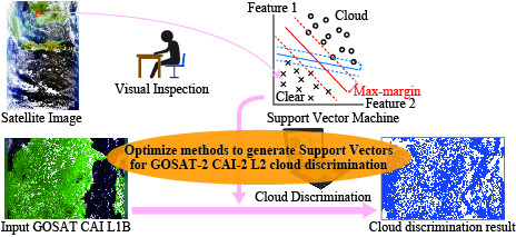
:Greenhouse gases Observing SATellite-2 (GOSAT-2) will be launched in fiscal year 2018. GOSAT-2 will be equipped with two sensors: the Thermal and Near-infrared Sensor for Carbon Observation (TANSO)-Fourier Transform Spectrometer 2 (FTS-2) and the TANSO-Cloud and Aerosol Imager 2 (CAI-2). CAI-2 is a push-broom imaging sensor that has forward- and backward-looking bands to observe the optical properties of aerosols and clouds and to monitor the status of urban air pollution and transboundary air pollution over oceans, such as PM2.5 (particles less than 2.5 micrometers in diameter). CAI-2 has important applications for cloud discrimination in each direction. The Cloud and Aerosol Unbiased Decision Intellectual Algorithm (CLAUDIA1), which applies sequential threshold tests to features is used for GOSAT CAI L2 cloud flag processing. If CLAUDIA1 is used with CAI-2, it is necessary to optimize the thresholds in accordance with CAI-2. However, CLAUDIA3 with support vector machines (SVM), a supervised pattern recognition method, was developed, and then we applied CLAUDIA3 for GOSAT-2 CAI-2 L2 cloud discrimination processing. Thus, CLAUDIA3 can automatically find the optimized boundary between clear and cloudy areas. Improvements in CLAUDIA3 using CAI (CLAUDIA3-CAI) continue to be made. In this study, we examined the impact of various support vectors (SV) on GOSAT-2 CAI-2 L2 cloud discrimination by analyzing (1) the impact of the choice of different time periods for the training data and (2) the impact of different generation procedures for SV on the cloud discrimination efficiency. To generate SV for CLAUDIA3-CAI from MODIS data, there are two times at which features are extracted, corresponding to CAI bands. One procedure is equivalent to generating SV using CAI data. Another procedure generates SV for MODIS cloud discrimination at the beginning, and then extracts decision function, thresholds, and SV corresponding to CAI bands. Our results indicated the following. (1) For the period from November to May, it is more effective to use SV generated from training data from February while for the period from June to October it is more effective to use training data from August; (2) In the preparation of SV, features obtained using MODIS bands are more effective than those obtained using the corresponding GOSAT CAI bands to automatically extract cloud training samples.
1. Introduction
There are few ground observation sites located in limited areas, though it is necessary to estimate and monitor greenhouse gas fluxes to cope with global warming caused by the greenhouse effect. However, satellites make observations at many points on the Earth; for example, Greenhouse gases Observing SATellite (GOSAT) records data at 56,000 points every 3 days. Thus, future satellite missions to monitor greenhouse gases are planned. GOSAT-2, the successor to GOSAT, will be launched in the fiscal year, 2018, to measure the global atmospheric CO2 (carbon dioxide), CH4 (methane), and CO (carbon monoxide) concentrations. GOSAT-2 will be equipped with two sensors: the Thermal and Near-infrared Sensor for Carbon Observation (TANSO)-Fourier Transform Spectrometer 2 (FTS-2) and the TANSO-Cloud and Aerosol Imager 2 (CAI-2) (Table 1).
The greenhouse gases column-averaged dry air mole fractions will be retrieved using the FTS-2. The CAI-2 will be used to observe the optical properties of aerosols and clouds, to monitor the status of urban air pollution and transboundary air pollution over oceans, and for cloud discrimination in the instantaneous field of view (IFOV) of the FTS-2 [1,2]. The Moderate Resolution Imaging Spectroradiometer (MODIS) cloud mask algorithm [3] is widely known as a highly accurate cloud discrimination algorithm for satellite images. The algorithm uses 22 bands in 36 MODIS spectral bands [4]. GOSAT CAI, however, uses only four bands from near ultraviolet (NUV) to short-wavelength infrared (SWIR). A cloud discrimination algorithm that maximally utilizes the small number of bands is needed for GOSAT CAI L2 cloud flag processing. Accordingly, the cloud and aerosol unbiased decision intellectual algorithm (CLAUDIA1) [5] with CAI was developed for cloud discrimination using GOSAT [6]. To improve the accuracy of estimates of atmospheric greenhouse gas concentrations, we need to refine the existing cloud discrimination algorithm, because the presence of clouds in the IFOV of the FTS-2 leads to incorrect estimates [7]. Therefore, a new cloud discrimination algorithm (CLAUDIA3) using support vector machines (SVM) [8] was developed [9], and then we applied CLAUDIA3 for GOSAT-2 CAI-2 L2 cloud discrimination processing. Verification and improvement of the processing method have been carried out and are still in progress, and these methods are evaluated in this study. Although the amount of observational data increases along with changes, such as the increased number of bands in GOSAT-2 TANSO-CAI-2, a ground system for the steady operational processing of GOSAT-2 data cannot be realized if the floor space significantly exceeds that of GOSAT. To deal with this problem, we previously evaluated the application of the graphics processing unit (GPU). These results indicated that the importance of the central processing unit (CPU) + GPU hybrid parallel processing for GOSAT-2 CAI-2 L2 cloud discrimination will increase in the future, as the data transfer speed between the host and the device memory becomes faster [10]. The observed time difference between the FTS-2 and CAI-2 may be greater than that between the FTS and CAI, because the CAI-2 is a push-broom imaging sensor with forward- and backward-looking bands. Thus, we proposed a method using CAI-2 cloud discrimination for screening cloud-contaminated FTS-2 data. The results indicated that it is necessary to add margins to the IFOV of the FTS-2 in a cloud discrimination image, depending on cloud movement by wind, to account for the time difference between CAI-2 and FTS-2 observations [11]. GOSAT and GOSAT-2 observations are made in sun-glint regions over the ocean, where specular reflection occurs and reflectance is high. In general, cloud discrimination in sun-glint regions is difficult, but either forward- or backward-looking bands of the CAI-2 can avoid sun-glint regions. We examined the difference between forward and backward cloud discrimination by applying CLAUDIA1 to Terra Multi-angle imaging Spectroradiometer (MISR) data. Over the ocean, cloud discrimination results that include no-sun-glint regions should be used for the retrieval of greenhouse gas column abundances. Over land, cloud discrimination results can be obtained with either band. Furthermore, the reason GOSAT-2 adopted to not use FTS-2 cloud discrimination, such as the A-Band Oxygen cloud screening algorithm (ABO2) [12], but instead use CAI-2 cloud discrimination has been described [13].
The CLAUDIA3 procedure with CAI (CLAUDIA3-CAI) can be roughly divided into the following steps.
- Perform supervised learning using SVM in a high-dimensional feature space of the training samples extracted from training images to determine the decision function, thresholds, and support vectors (SV).
- Perform cloud discrimination for input images, using the decision function, thresholds, and SV.
In this study, we performed two analyses to clarify the impact of the use of different SV on GOSAT-2 CAI-2 L2 cloud discrimination.
- We examined the impact of the choice of the collection period for the training data.
- We examined the impact of different SV generation procedures.
The present article is organized as follows: Section 2 describes the study areas, data, and analysis procedures used in the present study. Two comparative analyses of the training data and SV generation procedures are described in Section 3. The results are discussed in Section 4. Future work is presented in Section 5.
2. Tools and Methodology
2.1. Study Area and Data
We used Terra MODIS L1B calibrated radiances 1 km (MOD021KM) products in February and August 2012 as training data. We used GOSAT CAI L1B products, which can be downloaded from GOSAT User Interface Gateway (GUIG, https://data.gosat.nies.go.jp), for various land cover types, from 2012 to 2014, as input data (Table 2, Figure 1) and GOSAT CAI L3 global reflectance distribution products to generate surface albedo data and to examine seasonal change of surface reflectance. Currently GUIG has been changed to GOSAT Data Archive Service (GDAS, https://data2.gosat.nies.go.jp/index_en.html).
Study areas were selected using the MODIS land cover type product (MCD12). Japan scenes include Tokyo, which is the most populous megacity [14]. The spatial resolution of the CAI L1B products (pixel size at the nadir) was 500 m and the image size was 2048 × 1355 pixels (approximately 1000 × 680 km). CAI L1B products included the Shuttle Radar Topography Mission’s (SRTM) 15 arc-seconds land/sea mask. For areas at latitudes of higher than ±60°, however, the mask of the USGS Global Land 1-KM AVHRR Project was used. Surface albedo data at 1/8 arc-degree resolution were generated from CAI L3 global reflectance distribution products.
2.2. SV Preparation Procedure
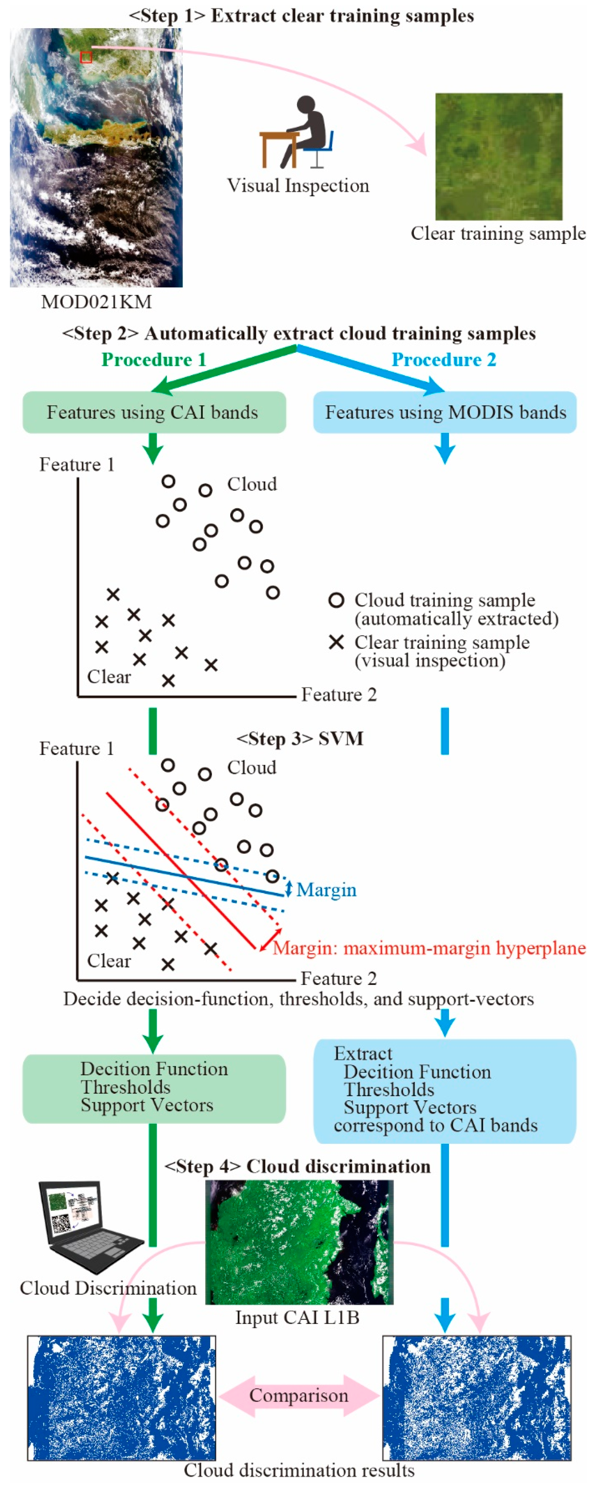
The SV preparation procedures included the steps shown in Figure 2.
- Extract clear training samples:Typical non-cloud-contaminated pixels were extracted as “clear training samples” by visual inspection from MOD021KM products for various land cover types.
- Automatically extract cloud training samples:“Cloud training samples” were automatically extracted under the assumption that pixels that were at sufficient distances from the clear training samples, based on Mahalanobis distances, were cloud-contaminated pixels.
- Decide decision function, thresholds, and SV:Supervised learning was performed using SVM, in a high-dimensional feature space for the extracted training samples, to determine the decision function, thresholds, and SV.
- Perform cloud discriminationCloud discrimination for input CAI L1B images was performed using the decision function, thresholds, and SV.
2.3. Analytical Procedure
We initially compared the CLAUDIA3-CAI results obtained using Terra MODIS data in February and August as training data. Next, we compared the CLAUDIA3-CAI results obtained using two types of SV, which were generated from the MODIS data following different procedures (Figure 2).
To generate SV for CLAUDIA3-CAI from MODIS data, there are two times at which features are extracted corresponding to CAI bands, i.e., at Step 2 (Procedure 1) or Step 3 (Procedure 2) in Figure 2. Procedure 1 is equivalent to generating SV using CAI data. Procedure 2 generates SV for MODIS cloud discrimination at the beginning, and then extracts decision functions, thresholds, and SV corresponding to CAI bands.
Finally, we compared the CLAUDIA3-CAI results obtained using MODIS and CAI data as training data.
3. Results
In this section, we summarize the results of three analyses of the impacts of SV. In this study, the “degree of agreement (D.A.)” was defined as the ratio of the number of pixels for which two CLAUDIA3-CAI results, obtained using different SV, agreed with respect to the number of pixels for an input image. “Overlook” was defined as the ratio of the number of pixels which a standard CLAUDIA3-CAI result judged cloudy, despite another clear result for the number of pixels for which the standard result was cloudy. “Overestimate” was defined as the ratio of the number of pixels judged as clear in the standard analysis, despite another result judged as cloudy for the number of pixels for which the standard result was clear. Because every CAI-2 band had the same swath width, but the swath width of CAI band 4 was different from that of bands 1–3, we used pixels in the swath range of CAI band 4. Each was defined by the following equations (the std subscript indicates standard results):
3.1. Results for Various Time Periods
To compare the CLAUDIA3-CAI results obtained using Terra MODIS data in February (Feb-SV) and August (Aug-SV) as training data, we used the comparative results for Feb-SV and Aug-SV. The SV generation procedure was Procedure 2.
Figure 3 shows monthly averages for the comparative results between Feb-SV and Aug-SV.
In Figure 3, for Overlook_2 and Overestimate_2, Feb-SV results were used as standard images, and Overlook_8 and Overestimate_8 used Aug-SV results as standard images. Overlook_2 was greater than Overlook_8 and Overestimate_8 was greater than Overestimate_2. Feb-SV results had a tendency to overestimate cloud regions and Aug-SV results had a tendency to overlook cloud regions. This can be explained by the darker images for Feb-SV than Aug-SV; the solar zenith angle is lower in February in the Northern hemisphere, which has a larger land area than the Southern hemisphere. In contrast, Aug-SV is prepared using brighter images and the solar zenith angle is higher in August in the Northern hemisphere. Therefore, the difference between results obtained using Feb-SV and Aug-SV is mainly explained by a trade-off relationship between the overestimation of results using Feb-SV and the underestimated results using Aug-SV.
In Australia, Japan, Borneo, and Algeria, there was no obvious seasonal variation. In Australia and Algeria, it was more effective to use Feb-SV throughout the year because Overlook_2 is strikingly great.
In Thailand, Overlook_2 was greater than Overestimate_8 from November to May, and Overestimate_8 was greater than Overlook_2 from June to October. For the period from November to May, it was more effective to use Feb-SV, while for the period from June to October it was more effective to use Aug-SV.
In Mongolia and Canada, we cannot generalize which SV was more effective, though there was seasonal variation.
In Alaska, it is more effective to use Aug-SV throughout the year excepting April because Overestimate_8 is strikingly great.
Overall, for the period from November to May, it was more effective to use Feb-SV while for the period from June to October it was more effective to use Aug-SV, when common SV is used in the global measurement.
3.2. Results Obtained for Various SV Generation Procedures
Table 4 shows the comparative results using the SV generated by Procedures 1 and 2, when using the SV generated by Procedure 1 as a standard.
In Australia and Algeria, the difference between Procedures 1 and 2 was less than 1%.
4. Discussion
In this section, we discuss the relationship between the seasonal variation in Figure 3 and the seasonal change of surface reflectance, and discuss the cause of high D.A. in Alaska and low D.A. in Thailand and Borneo Island.
4.1. Relationshp between the Seasonal Variation and the Seasonal Change of Surface Reflectance
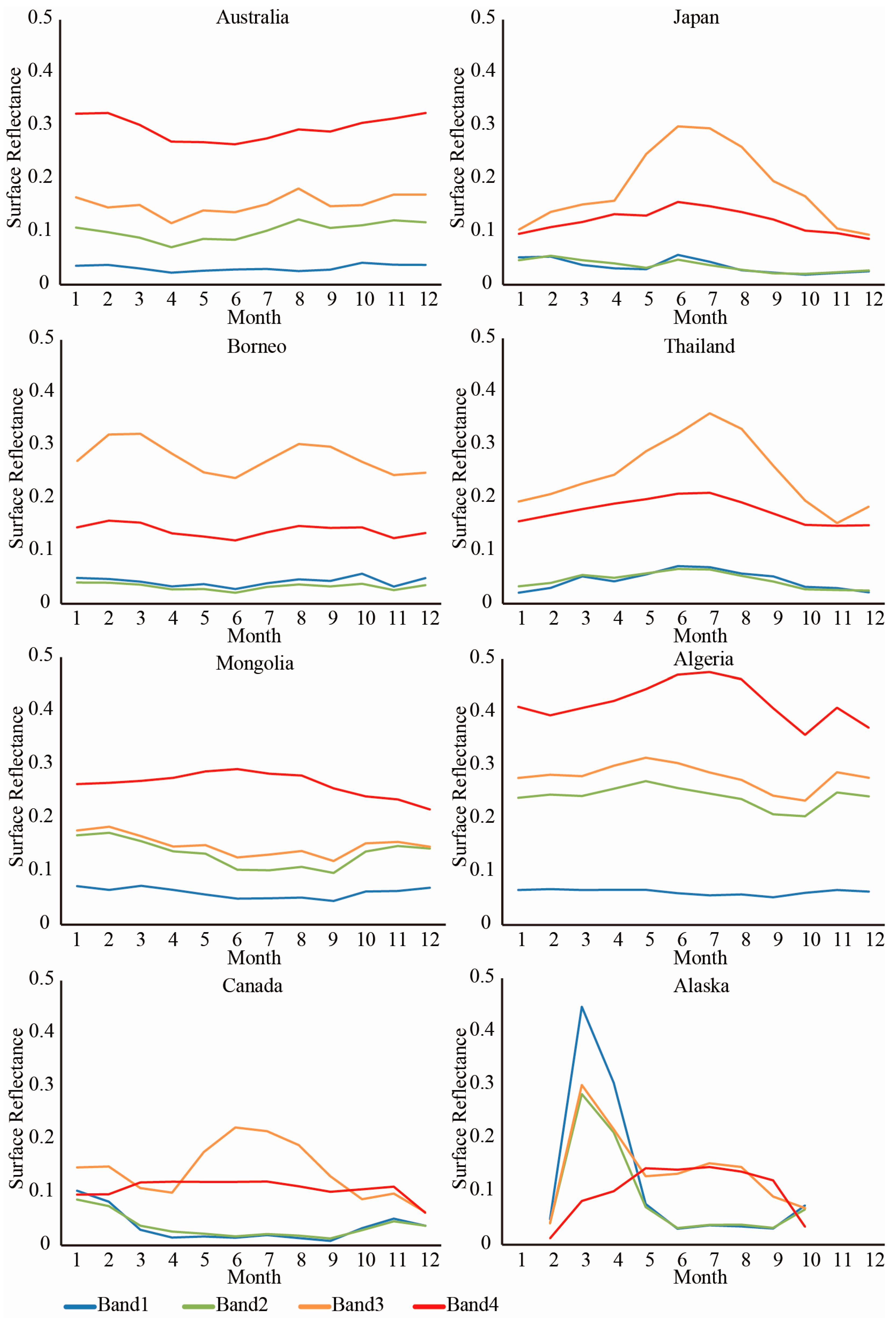
Figure 4 shows the change of surface reflectance in each band, and Figure 5 shows the global surface reflectance generated from CAI L3 global reflectance distribution products.
In Australia, the surface reflectance of Band 2 increased with that of Band 3 from April to August. It was caused by changing to dry land, corresponding to a reduction of vegetation from April to August because Australia is in the Southern hemisphere. For this reason, it is considered that there was tendency to overlook clouds using Aug-SV.
In Japan, surface reflectance of Band 3 was particularly higher than the other bands from May to October. It was caused by seasonal vegetation change. Meanwhile there was no obvious seasonal variation in Figure 3. It is difficult to determine the reason because cloud discrimination results depend on several features.
In Borneo, there was no obvious seasonal variation of surface reflectance.
In Thailand, surface reflectance of Band 3 was particularly higher than the other bands from May to October as Japan. For the reason, it is considered that there was a tendency to overestimate clouds from June to October, using Feb-SV, and to overlook clouds from November to May, using Aug-SV.
In Mongolia, the surface reflectance of Bands 2 and 3 from October to April was higher than that from May to September, while the surface reflectance of Band 4 from October to April was lower than that from May to September. It was caused by snow. It is considered that snow influenced the seasonal variation in Figure 3.
In Algeria, the surface reflectance of Bands 2–4 changed in the same way. It is considered that the lower surface reflectance in October, compared to the other months, influenced high Overlook, using Feb-SV and Aug-SV in October.
In Canada, the surface reflectance of Band 3 was particularly higher than the other bands, from May to September. It was caused by seasonal vegetation change. Meanwhile, the surface reflectance of Bands 2 and 3 from October to March was higher than that from April to September, while the surface reflectance of Band 4 from December to February was lower than that from March to November. It was caused by snow.
In Alaska, there was the same trend as Canada. Meanwhile the surface reflectance of Bands 1–3 from March to April was particularly higher than the other months. It might be caused by clouds. CAI L3 global reflectance distribution products were generated by collecting the image data with minimum reflectance from the CAI L1 data for 30 days (10 recurrent cycles) to remove clouds [15]. However, clouds remained when it was cloudy in all 10 images.
4.2. Cause of High D.A. in Alaska and Low D.A. in Thailand and Borneo Island
Figure 6 shows an example of comparative results for Alaska.
Since the CAI is not equipped with any thermal infrared bands, cloud discrimination based on the temperature at the top of clouds is not feasible. Accordingly, it is difficult to discriminate optically thin clouds and to discriminate between clouds and ice or snow. Thus, both Procedures 1 and 2 misidentified ice and snow as clouds. The difference or coincidence between Procedures 1 and 2 in Alaska was attributed to this source of error.
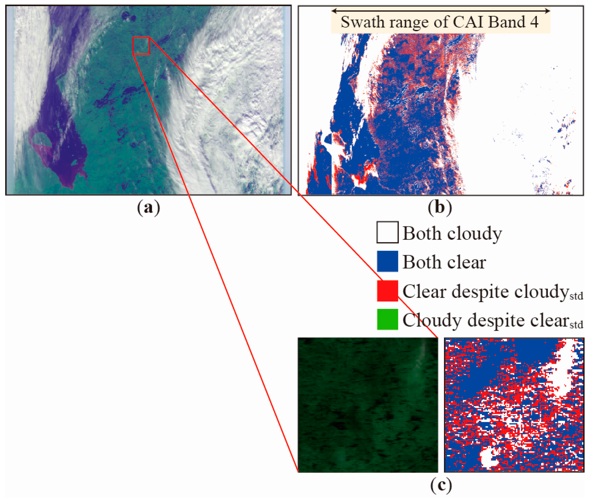
There was a bigger difference between methods in Thailand and Borneo Island, nearly 7%, than those observed in other study areas. Figure 7 shows an example of comparative results for Borneo.
Procedure 1 had a tendency to overlook optically thin clouds in comparison with Procedure 2.
Figure 8 shows an example of comparative results for Canada. Procedure 1 had a tendency to misjudge bright surfaces as clouds to a greater extent than Procedure 2.
5. Conclusions
In this study, we performed two analyses to clarify the impacts of different SV on GOSAT-2 CAI-2 L2 cloud discrimination.
Comparative CLAUDIA3-CAI results, using Terra MODIS data in February (Feb-SV) and August (Aug-SV) as training data, indicated that we should use Feb-SV from November to May and Aug-SV from June to October, when common SV is used in the global measurements. Whether the combination of Feb-SV and Aug-SV, and the interval of 6 months are optimal, are subjects for future examinations.
We compared SV generated by Procedures 1 and 2. Procedure 1 was equivalent to generating SV using CAI data. Procedure 2 generated SV for MODIS cloud discrimination at the beginning, and then extracted a decision function, thresholds, and SV corresponding to CAI bands. The comparative results indicated that the cloud discrimination accuracy was better for Procedure 2 than Procedure 1. Cloud training samples were automatically extracted by features using CAI bands at Step 2 in Procedure 1. Thus, Procedure 1 might extract clear-sky bright surfaces and cannot extract optically thin clouds as cloud training samples. These results provide a basis for decisions about training data sampling. It is necessary to add a new category of clear training samples for clear-sky bright surfaces that are misjudged as clouds, and it may be useful to intentionally add clouds on bright surfaces to cloud training samples.
Currently, the preparation of training data extracted from CAI data is in progress to evaluate differences between the use of Terra Moderate Resolution Imaging Spectroradiometer (MODIS) data and GOSAT CAI data as training data. If the comparative results indicate that using GOSAT CAI data as training data is better, SV for GOSAT-2 must be generated using GOSAT-2 CAI-2 data themselves as training data, otherwise, the SV generated by Procedure 2 in this study will be used for GOSAT-2 CAI-2 L2 cloud discrimination processing. Furthermore, we will study the application of the bands added in CAI-2 for retrieval of aerosol properties to cloud discrimination.
Acknowledgments
This research was mainly supported by the GOSAT-2 Project at the National Institute for Environmental Studies (NIES), Japan (2016). A part of this research is based on results obtained from a project commissioned by the New Energy and Industrial Technology Development Organization (NEDO), Japan. The authors would like to thank the GOSAT Project and GOSAT-2 Project for helpful comments as well as Ryosuke Kudo and Takuya Yamagishi for assistance with visual inspections.
Author Contributions
Yu Oishi, Haruma Ishida, Takashi Y. Nakajima, Ryosuke Nakamura, and Tsuneo Matsunaga conceived and designed the studies; Yu Oishi performed evaluations and analyzed the data; Haruma Ishida contributed analysis tools; Yu Oishi wrote the paper.
Conflicts of Interest
The authors declare no conflict of interest. The founding sponsors had no role in the design of the study; in the collection, analyses, or interpretation of data; in the writing of the manuscript, and in the decision to publish the results.
References
- GOSAT-2 Project at the National Institute for Environmental Studies, about GOSAT-2. Available online: www.gosat-2.nies.go.jp (accessed on 10 October 2017).
- Algorithm Theoretical Basis Document (ATBD) for CO2 and CH4 Column Amounts Retrieval from GOSAT TANSO-FTS SWIR. Available online: https://data2.gosat.nies.go.jp/doc/documents/ATBD_FTSSWIRL2_V2.0_en.pdf (accessed on 10 October 2017).
- Ackerman, S.; Strabala, K.; Menzel, P.; Frey, R.; Moeller, C.; Guemley, L. Discriminating clear sky from clouds with MODIS. J. Geophys. Res. 1998, 103, 32141–32157. [Google Scholar] [CrossRef]
- Discriminating Clear-Sky from Cloud with MODIS Algorithm Theoretical Basis Document (MOD35). Available online: http://modis-atmos.gsfc.nasa.gov/_docs/MOD35_ATBD_Collection6.pdf (accessed on 24 November 2017).
- Ishida, H.; Nakajima, T.Y. Development of an unbiased cloud detection algorithm for a spaceborne multispectral imager. J. Geophys. Res. 2009, 114. [Google Scholar] [CrossRef]
- Ishida, H.; Nakajima, T.Y.; Yokota, T.; Kikuchi, N.; Watanabe, H. Investigation of GOSAT TANSO-CAI cloud screening ability through an intersatellite comparison. J. Appl. Meteorol. Climatol. 2011, 50, 1571–1586. [Google Scholar] [CrossRef]
- Uchino, O.; Kikuchi, N.; Sakai, T.; Morino, I.; Yoshida, Y.; Nagai, T.; Shimizu, A.; Shibata, T.; Yamazaki, A.; Uchiyama, A.; et al. Influence of aerosols and thin cirrus clouds on the GOSAT-observed CO2: A case study over Tsukuba. Atmos. Chem. Phys. 2012, 12, 3393–3404. [Google Scholar] [CrossRef]
- Vapnik, V.; Lerner, A. Pattern recognition using generalized portrait method. Autom. Remote Control 1963, 24, 774–780. [Google Scholar]
- Ishida, H.; Oishi, Y.; Morita, K.; Moriwaki, K.; Nakajima, T.Y. Development of a support vector machine based cloud detection method for MODIS with the adjustability to various conditions. Remote Sens. Environ. 2017, in press. [Google Scholar]
- Oishi, Y.; Hiraki, K.; Yokota, Y.; Sawada, Y.; Murakami, K.; Kamei, A.; Yoshida, Y.; Matsunaga, T. Usability evaluation of GPU for GOSAT-2 TANSO-CAI-2 L2 cloud flag processing. J. Remote Sens. Soc. Jpn. 2015, 35, 173–183, (In Japanese with English Abstract). [Google Scholar] [CrossRef]
- Oishi, Y.; Nagao, T.M.; Ishida, H.; Nakajima, T.Y.; Matsunaga, T. Preliminary study of a method using the GOSAT-2 CAI-2 cloud discrimination for screening of cloud-contaminated FTS-2 data. J. Remote Sens. Soc. Jpn. 2015, 35, 299–306, (In Japanese with English Abstract). [Google Scholar] [CrossRef]
- Taylor, T.E.; O’Dell, C.W.; O’Brien, D.M.; Kikuchi, N.; Yokota, T.; Nakajima, T.Y.; Ishida, H.; Crisp, D.; Nakajima, T. Comparison of cloud-screening methods applied to GOSAT near-infrared spectra. IEEE Trans. Geosci. Remote Sens. 2012, 50, 295–309. [Google Scholar] [CrossRef]
- Oishi, Y.; Nakajima, T.Y.; Matsunaga, T. Difference between forward- and backward-looking bands of GOSAT-2 CAI-2 cloud discrimination using Terra MISR data. Int. J. Remote Sens. 2016, 37, 1115–1126. [Google Scholar] [CrossRef]
- The World’s Cities in 2016. Available online: http://www.un.org/en/development/desa/population/publications/pdf/urbanization/the_worlds_cities_in_2016_data_booklet.pdf (accessed on 7 November 2017).
- NIES GOSAT TANSO-CAI Level 3 Data Product Format Description. Available online: https://data2.gosat.nies.go.jp/GosatDataArchiveService/doc/GU/GOSAT_ProductDescription_33_CAIL3_V3.01_en.pdf (accessed on 17 November 2017).
Figure 1.
Study areas. Black rectangles indicate the locations of CAI frames.
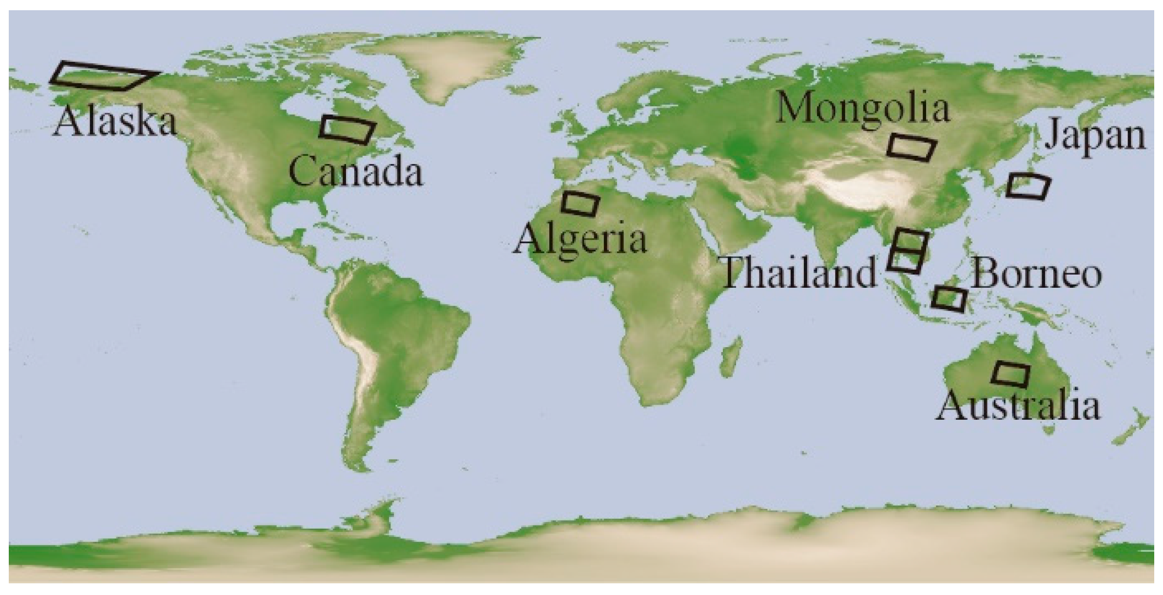
Figure 2.
Analytical procedure to examine the impact of different SV generation procedures using MODIS data.
Figure 2.
Analytical procedure to examine the impact of different SV generation procedures using MODIS data.

Figure 3.
Monthly averages of “degree of agreement (D.A.)”, “Overlook”, and “Overestimate” in a comparative analysis using Feb-SV (February support vector) and Aug-SV (August support vector). For Overlook_2 and Overestimate_2, Feb-SV results were used as standard images, and Overlook_8 and Overestimate_8 used Aug-SV results as standard images.
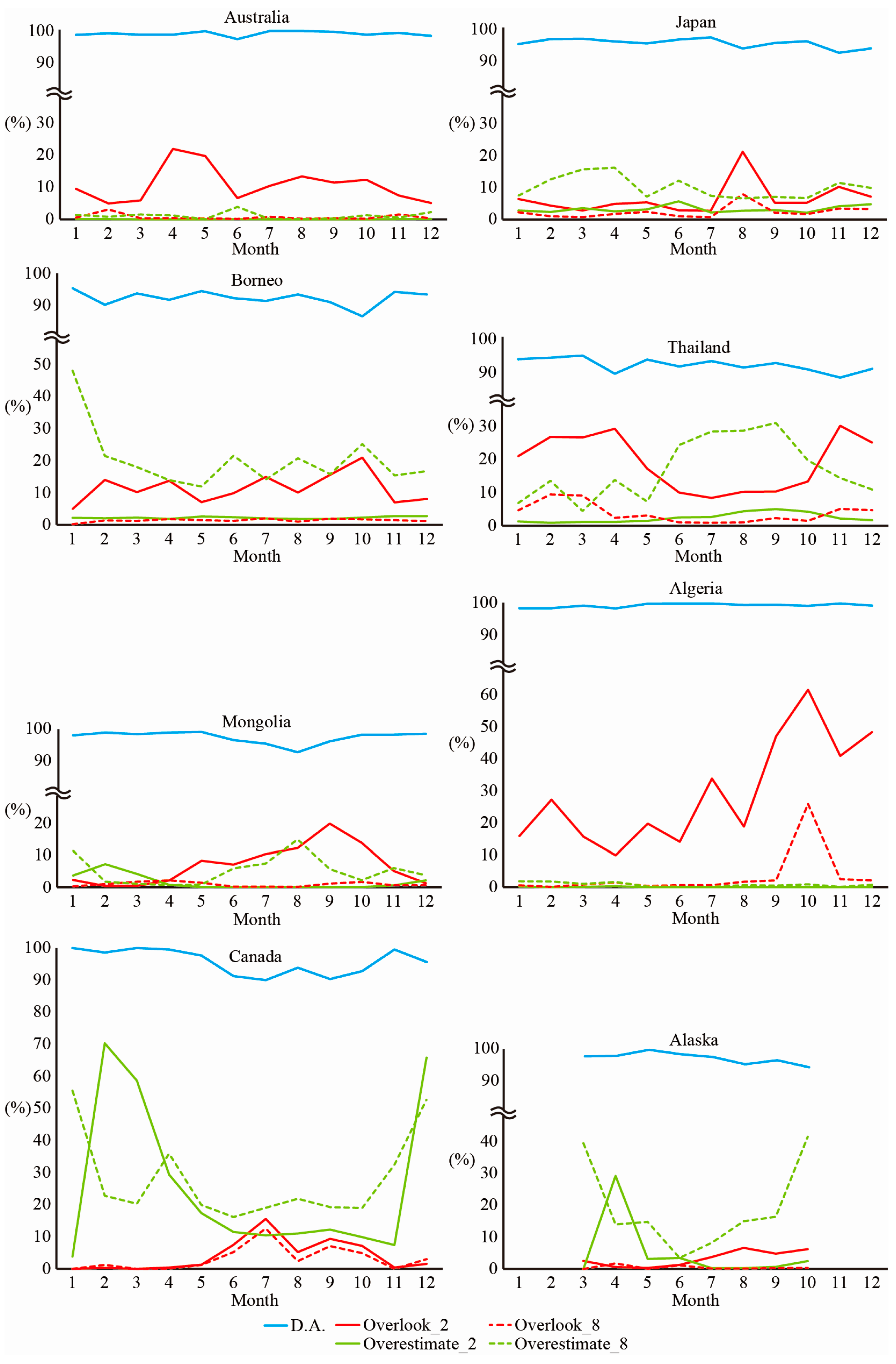
Figure 4.
Change of surface reflectance in each band (Band 1: 0.38 nm; Band 2: 0.67 nm; Band 3: 0.87 nm; Band 4: 1.6 μm).
Figure 4.
Change of surface reflectance in each band (Band 1: 0.38 nm; Band 2: 0.67 nm; Band 3: 0.87 nm; Band 4: 1.6 μm).

Figure 5.
Change of global surface reflectance (R: Band 2; G: Band 3; B: Band 1).
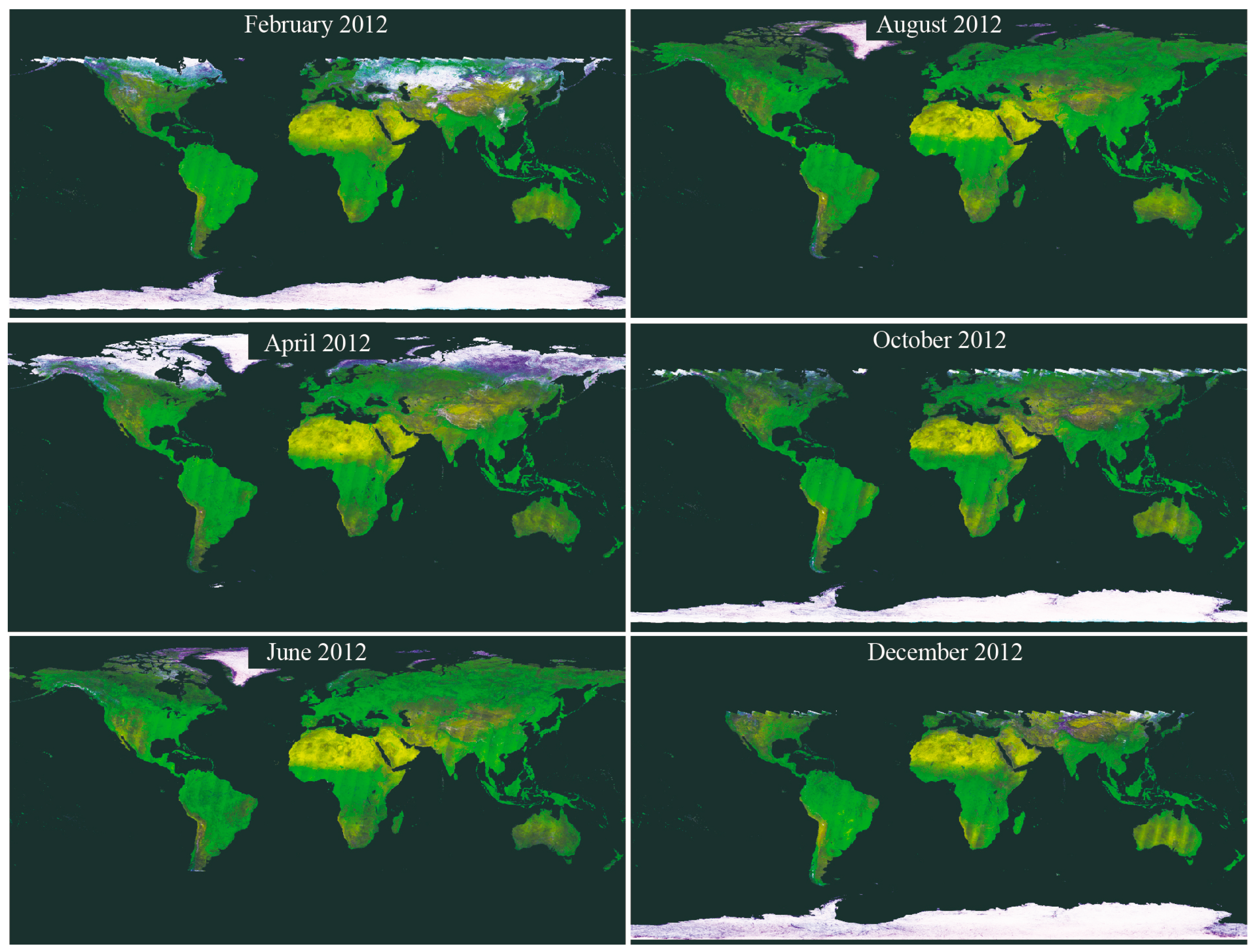
Figure 6.
Comparative results for Alaska on 1 March 2014. (a) Input CAI L1B product (R: Band 2, G: Band 3, B: Band 1); (b) Comparative results for the SV generated by Procedures 1 and 2 when using the SV generated by Procedure 1 as a standard. The right lower border is caused by the conversion of features from land or water cloud tests to polar cloud tests.
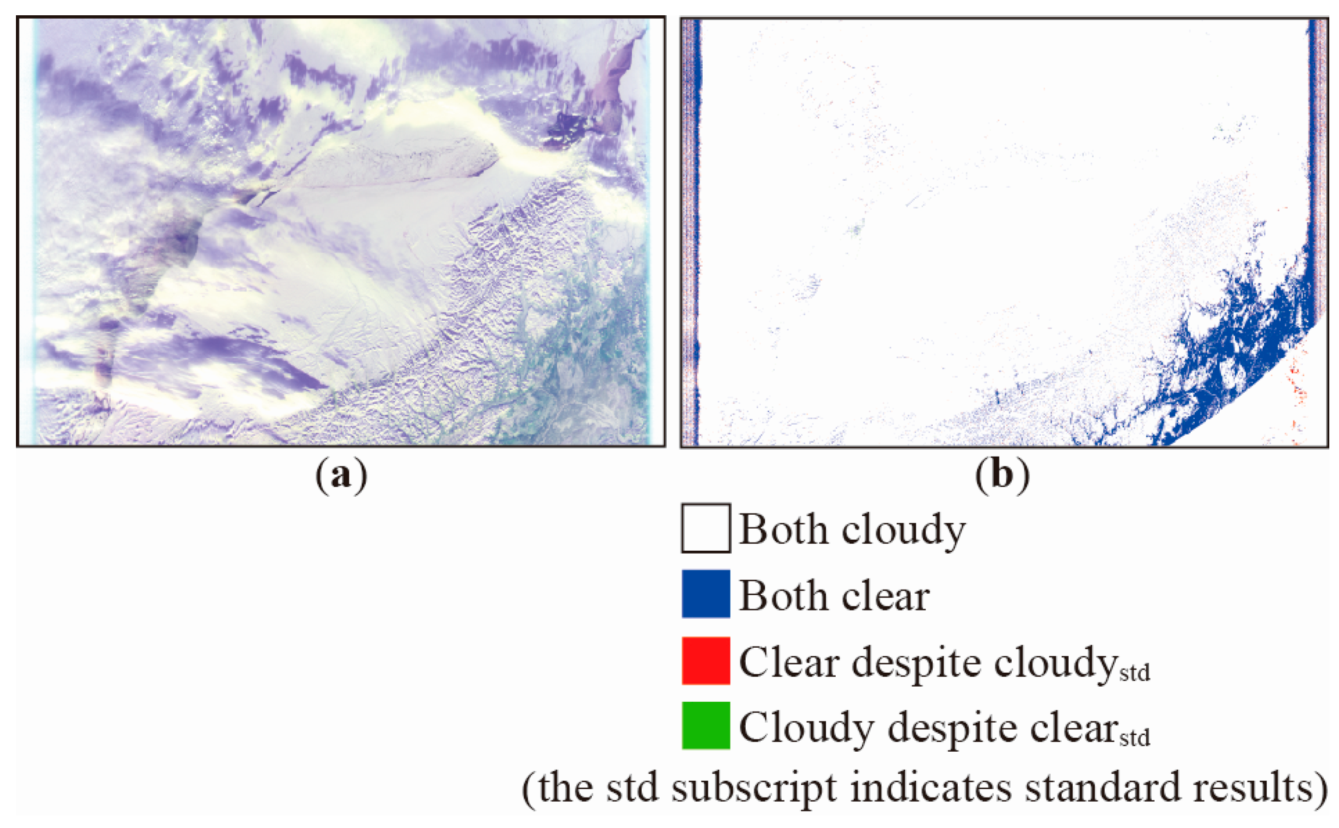
Figure 7.
Comparative results for Borneo Island on 2 June 2012. (a) Input CAI L1B product (R: Band 2, G: Band 3, B: Band 1); (b) Comparative results using SV generated by Procedures 1 and 2 when using the SV generated by Procedure 1 as a standard; (c) Enlarged figures of (a) and (b).
Figure 7.
Comparative results for Borneo Island on 2 June 2012. (a) Input CAI L1B product (R: Band 2, G: Band 3, B: Band 1); (b) Comparative results using SV generated by Procedures 1 and 2 when using the SV generated by Procedure 1 as a standard; (c) Enlarged figures of (a) and (b).

Figure 8.
Comparative results for Canada on 1 October 2012. (a) Input CAI L1B product (R: Band 2, G: Band 3, B: Band 1); (b) Comparative results using SV generated by Procedures 1 and 2 when using the SV generated by Procedure 1 as a standard; (c) Enlarged figures of (a) and (b).
Figure 8.
Comparative results for Canada on 1 October 2012. (a) Input CAI L1B product (R: Band 2, G: Band 3, B: Band 1); (b) Comparative results using SV generated by Procedures 1 and 2 when using the SV generated by Procedure 1 as a standard; (c) Enlarged figures of (a) and (b).


Table 1.
Specifications of Greenhouse gases Observing SATellite (GOSAT) Cloud and Aerosol Imager (CAI) and GOSAT-2 CAI-2.
Table 1.
Specifications of Greenhouse gases Observing SATellite (GOSAT) Cloud and Aerosol Imager (CAI) and GOSAT-2 CAI-2.
| Specifications of GOSAT CAI | ||||
| Band | Spectral Coverage (μm) | Spatial Resolution (m) | Swath (km) | |
| 1 | 0.370–0.390 | 500 | 1000 | |
| 2 | 0.664–0.684 | 500 | 1000 | |
| 3 | 0.860–0.880 | 500 | 1000 | |
| 4 | 1.555–1.645 | 1500 | 750 | |
| Specifications of GOSAT-2 CAI-2 | ||||
| Band | Spectral Coverage (μm) | Spatial Resolution (m) | Viewing Angle (°) | Swath (km) |
| 1 | 0.333–0.353 | 460 | +20 (Forward) | 920 |
| 2 | 0.433–0.453 | |||
| 3 | 0.664–0.684 | |||
| 4 | 0.859–0.879 | |||
| 5 | 1.585–1.675 | 920 | ||
| 6 | 0.370–0.390 | 460 | −20 (Backward) | |
| 7 | 0.540–0.560 | |||
| 8 | 0.664–0.684 | |||
| 9 | 0.859–0.879 | |||
| 10 | 1.585–1.675 | 920 | ||
Table 2.
GOSAT CAI L1B products evaluated in this study. Land-cover was derived from the MODIS land cover type product (MCD12).
Table 2.
GOSAT CAI L1B products evaluated in this study. Land-cover was derived from the MODIS land cover type product (MCD12).
| Location (CAI Path_Frame) | Data Period | Land Cover |
|---|---|---|
| Australia (4_35) | 3 April 2012–3 March 2014 | Open shrublands |
| Japan (5_25) | 1 April 2012–1 March 2014 | Mixed forests |
| Borneo (7_31) | 3 April 2012–3 March 2014 | Evergreen broadleaf forest |
| Thailand 1 (9_28) | 2 April 2012–2 March 2014 | Cropland/natural vegetation |
| Thailand 2 (9_29) | 2 April 2012–2 March 2014 | Cropland/natural vegetation |
| Mongolia (22_26) | 3 April 2012–3 March 2014 | Grasslands |
| Algeria (22_26) | 3 April 2012–3 March 2014 | Barren or sparsely vegetated |
| Canada (32_22) | 1 April 2012–1 March 2014 | Evergreen needleleaf forest |
| Alaska (43_19) | 1 April 2012–1 March 2014 | Open shrublands |
Table 3.
Features using MODIS bands and CAI bands. Rwavelength and Twavelength denote the top of atmosphere (TOA) reflectance and brightness temperature, respectively, at a wavelength. The definitions of NDSI, NDVI, and Split window are (R0.66 − R1.64)/(R0.66 + R1.64), (R0.87 − R0.66)/(R0.87 + R0.66), and T11.0 − T12.0, respectively.
| Features Using MODIS Bands | Features Using CAI Bands |
|---|---|
| NDSI | R0.66 |
| R0.66 | R0.87 |
| R0.87 | R0.87/R0.66 |
| R0.87/R0.66 | NDVI |
| NDVI | R0.87/R1.64 |
| T13.9 | |
| T13.3 − T11.0 | |
| Split window | |
| T11.0 − T8.6 | |
| T11.0 − T3.9 | |
| R1.38 | |
| R0.905/R0.935 | |
| R0.87/R1.64 | |
| R1.24/R0.55 |
Table 4.
Average and standard deviation (in parentheses) of degree of agreement (D.A.), Overlook, and Overestimate for each study area.
Table 4.
Average and standard deviation (in parentheses) of degree of agreement (D.A.), Overlook, and Overestimate for each study area.
| Location (CAI Path_Frame) | D.A. (%) | Overlook (%) | Overestimate (%) |
|---|---|---|---|
| Australia (4_35) | 99.4 (0.9) | 0.3 (0.3) | 0.8 (1.3) |
| Japan (5_25) | 97.3 (1.3) | 2.8 (2.3) | 3.2 (4.1) |
| Borneo (7_31) | 93.1 (4.6) | 2.4 (2.5) | 10.5 (11.9) |
| Thailand 1 (9_28) | 93.3 (4.5) | 6.7 (8.3) | 13.0 (18.0) |
| Thailand 2 (9_29) | 95.0 (2.0) | 6.8 (7.9) | 7.9 (9.8) |
| Mongolia (10_23) | 97.6 (2.1) | 1.1 (2.0) | 3.7 (3.9) |
| Algeria (22_26) | 99.3 (1.4) | 1.1 (3.0) | 0.7 (1.5) |
| Canada (32_22) | 96.7 (3.0) | 1.3 (3.0) | 15.6 (14.8) |
| Alaska (43_19) | 98.8 (0.8) | 1.1 (0.9) | 4.1 (7.3) |
© 2017 by the authors. Licensee MDPI, Basel, Switzerland. This article is an open access article distributed under the terms and conditions of the Creative Commons Attribution (CC BY) license (http://creativecommons.org/licenses/by/4.0/).
Share and Cite
MDPI and ACS Style
Oishi, Y.; Ishida, H.; Nakajima, T.Y.; Nakamura, R.; Matsunaga, T. The Impact of Different Support Vectors on GOSAT-2 CAI-2 L2 Cloud Discrimination. Remote Sens. 2017, 9, 1236. https://doi.org/10.3390/rs9121236
AMA Style
Oishi Y, Ishida H, Nakajima TY, Nakamura R, Matsunaga T. The Impact of Different Support Vectors on GOSAT-2 CAI-2 L2 Cloud Discrimination. Remote Sensing. 2017; 9(12):1236. https://doi.org/10.3390/rs9121236
Chicago/Turabian StyleOishi, Yu, Haruma Ishida, Takashi Y. Nakajima, Ryosuke Nakamura, and Tsuneo Matsunaga. 2017. "The Impact of Different Support Vectors on GOSAT-2 CAI-2 L2 Cloud Discrimination" Remote Sensing 9, no. 12: 1236. https://doi.org/10.3390/rs9121236
Note that from the first issue of 2016, this journal uses article numbers instead of page numbers. See further details here.