Estimating Land Surface Temperature from Feng Yun-3C/MERSI Data Using a New Land Surface Emissivity Scheme


1
State Key Laboratory of Remote Sensing Science, Jointly Sponsored by Beijing Normal University and Institute of Remote Sensing and Digital Earth of Chinese Academy of Sciences, Beijing 100875, China
2
Institute of Remote Sensing Science and Engineering, Faculty of Geographical Science, Beijing Normal University, Beijing 100875, China
3
Department of Geographical Sciences, University of Maryland, College Park, MD 20742, USA
*
Author to whom correspondence should be addressed.
Remote Sens. 2017, 9(12), 1247; https://doi.org/10.3390/rs9121247
Submission received: 2 November 2017
/
Revised: 29 November 2017
/
Accepted: 29 November 2017
/
Published: 1 December 2017
(This article belongs to the Special Issue Advances in Quantitative Remote Sensing in China – In Memory of Prof. Xiaowen Li)
Abstract
:Land surface temperature (LST) is a key parameter for a wide number of applications, including hydrology, meteorology and surface energy balance. In this study, we first proposed a new land surface emissivity (LSE) scheme, including a lookup table-based method to determine the vegetated surface emissivity and an empirical method to derive the bare soil emissivity from the Global LAnd Surface Satellite (GLASS) broadband emissivity (BBE) product. Then, the Modern Era Retrospective-Analysis for Research and Applications (MERRA) reanalysis data and the Feng Yun-3C/Medium Resolution Spectral Imager (FY-3C/MERSI) precipitable water vapor product were used to correct the atmospheric effects. After resolving the land surface emissivity and atmospheric effects, the LST was derived in a straightforward manner from the FY-3C/MERSI data by the radiative transfer equation algorithm and the generalized single-channel algorithm. The mean difference between the derived LSE and field-measured LSE over seven stations is approximately 0.002. Validation of the LST retrieved with the LSE determined by the new scheme can achieve an acceptable accuracy. The absolute biases are less than 1 K and the STDs (RMSEs) are less than 1.95 K (2.2 K) for both the 1000 m and 250 m spatial resolutions. The LST accuracy is superior to that retrieved with the LSE determined by the commonly used Normalized Difference Vegetation Index (NDVI) threshold method. Thus, the new emissivity scheme can be used to improve the accuracy of the LSE and further the LST for sensors with broad spectral ranges such as FY-3C/MERSI.

1. Introduction
Land surface temperature (LST) is one of the key parameters in the land surface physical processes at regional and global scales, integrating the interactions between the surface and atmosphere and all energy exchanges between the atmosphere and the land [1,2]. LST plays a significant role in many research fields, such as weather forecasting, global ocean circulation and climate change research [3]. Remote sensing is a unique way of obtaining the LST at regional and global scales. Three kinds of algorithms have been proposed in the past decades to derive the LST from satellite data [4,5], i.e., the single-channel algorithm [6,7,8], the split-window (SW) algorithm [1,9,10,11] and the multi-channel algorithm [12,13]. With these versatile algorithms, many LST products have been produced from different satellite data, such as the Advanced Spaceborne Thermal Emission and Reflection Radiometer (ASTER) [14,15], Moderate Resolution Imaging Spectroradiometer (MODIS) [1,16], Visible Infrared Imaging Radiometer Suite (VIIRS) [10,17], Geostationary Operational Environmental Satellites (GOES) [18,19] and Spinning Enhanced Visible and Infrared Imager (SEVIRI) [20]. Those LST products have been widely used for monitoring urban heat islands [21,22] and volcanoes [23,24,25], detecting forest fires [26,27], and so on.
FengYun-3C (FY-3C) satellites are China’s second-generation polar-orbiting meteorological satellites. The Medium Resolution Spectral Imager (MERSI) is the instrument onboard the FY-3C, with 4 of 19 visible/shortwave channels and 1 thermal infrared (TIR) channel are set for 250 m spatial resolution, with other channels for 1 km spatial resolution. FY-3C/MERSI also provides 1000 m radiance data interpolated from the original 250 m data. Thus, we can obtain 250 m and 1000 m spatial resolution thermal infrared data from FY-3C/MERSI. FY-3C/MERSI provides a new data source for the retrieval of LST and meteorology monitoring. However, to our knowledge, an operational FY-3C/MERSI LST product is unavailable.
For the sensor with only one TIR channel, a set of LST retrieval algorithms, such as the radiative transfer equation algorithm [8,28], the mono-window algorithm [6] and the generalized single-channel algorithm [7], have been developed for estimating the LST. According to the validation results obtained from four Surface Radiation Budget Network (SURFRAD) sites by Yu et al. [29], the radiative transfer equation algorithm has the highest accuracy, and the root mean square error is less than 1 k. Additionally, the study by Windahl and Beurs [30] verified the precision of the radiative transfer equation method, mono-window algorithm and generalized single-channel algorithm. The accuracy of the three algorithms decreased with the increase of water vapor content, and the radiative transfer equation method has a higher precision under a high water vapor content. The research of Jiménez-Muñoz et al. [31] indicated that the accuracy of the generalized single-channel algorithm is below 1 K when the water vapor content was lower than 2 g/cm2. The effective mean atmospheric temperatures in the mono-window algorithm are often estimated from the empirical formula with the near-surface air temperature, and this may be not suitable for some special study areas [32]. Thus, both the radiative transfer equation algorithm and the generalized single-channel algorithm are the potential LST retrieval algorithms for FY-3C/MERSI.
The accuracy of the single channel algorithm depends on the accuracy of the atmospheric correction and land surface emissivity (LSE). At present, the Normalized Difference Vegetation Index (NDVI) threshold method [33], the Vegetation Cover Method (VCM) [3] and the classification-based method [34] are widely used in the single channel algorithms. However, these techniques present several limitations. LSE based on the classification-based method cannot reflect the land cover changes [35]. For example, the MODIS LST products (collection 5) underestimate the LST in an arid area of northwest China, due to an overestimation of the LSE by the classification-based method [36]. Therefore, an accurate LSE scheme is the prerequisite of accurate LST retrieval. In addition to the determination accuracy of the land surface emissivity, the precision of the atmospheric correction also affects the results of the LST. Most of the single channel algorithms were developed without considering the effect of the view zenith angle; this will introduce a large error into the results of the sensor with a large view zenith angle [32]. Given that the view zenith angle of FY-3C/MERSI can reach up to 55 degrees, we will conduct an angular dependent atmospheric correction.
This study aims to accurately estimate the LST from the FY-3C/MERSI data using a more realistic LSE scheme. The structure of this paper is arranged as follows: Section 2 introduces the data used in this study and the estimation of the ground LST. Section 3 describes the methodology used in this study, including a new LSE scheme, atmospheric correction and the determination of the LST. The results and analysis are presented in Section 4. A discussion is provided in Section 5, and the main conclusions are summarized in Section 6.
2. Data
2.1. Satellite Products
The FY-3C/MERSI images, Global LAnd Surface Satellite (GLASS) broadband emissivity (BBE) product, GLASS leaf area index (LAI) product, MODIS Surface Reflectance data (MOD09GQ) and MODIS Land Cover data (MCD12Q1) were used to estimate the land surface temperature. Nine FY-3C/MERSI images ranging from 17 July 2014 to 6 October 2014 were obtained in this study. For the convenience of registration, the calibrated MERSI 1000 m resolution earth viewing data was used after calibration. The land surface reflectance, land cover or LAI products from FY-3C/MERSI are unavailable; therefore, the MOD09GQ, MCD12Q1 and GLASS LAI were used for the LST retrieval from FY-3C/MERSI. The FY-3C/MERSI images were re-projected to the projection of MOD09GQ. All the satellite products used were resampled to 1 km resolution to match the spatial resolution of the FY-3C/MERSI data.
The MOD09GQ Version 6 product provides an estimate of the surface spectral reflectance of the Terra MODIS 250 m data corrected for the atmospheric conditions such as gases, aerosols, and Rayleigh scattering. The MOD09GQ were used to calculate the NDVI and then identify the vegetated surfaces. The MODIS Land Cover product (MCD12Q1) is an annual land cover dataset with a 500 m spatial resolution, which contains five classification schemes. The International Geosphere Biosphere Program (IGBP) global vegetation classification scheme was selected in this paper to determine the leaf emissivity of vegetated surfaces.
The GLASS BBE product [37] was derived from the Advanced Very High Resolution Radiometer (AVHRR) and MODIS data using the newly developed algorithms [38,39]. The GLASS LAI product was generated using a general regression neural network (GRNN) from the MODIS surface reflectance data [40]. Both GLASS BBE and LAI products have spatial and temporal resolutions of 1 km and eight days, respectively. Detailed information for the GLASS product can be found in Liang et al. [37]. The GLASS BBE and the GLASS LAI products were used for estimating the LSE for FY-3C/MERSI.
2.2. Ground Measurements
The Heihe Watershed Allied Telemetry Experimental Research (HiWATER) [41,42] was performed in the Heihe River Basin, which is a typical inland river basin in northwest China. In this study, three datasets were selected from this experiment: the dataset of the thermal infrared spectrum observed by BOMEM MR304 in the middle reaches of the Heihe River Basin [43], the dataset of the hydrometeorological observation network (automatic weather station, 2014) [44] and the dataset of infrared temperature in the Zhanye Airport desert [45].
The surface-leaving radiance of the different components of land surfaces (soil, sand, corn leaf, soybean leaf, apple leaf, etc.) and atmospheric downward radiance were measured by ABB BOMEM MR304 spectroradiometers and a diffuse gold plate [36]. The emissivity spectra in the range of 8~14 µm with a spectral resolution of 1 cm−1 were retrieved using the Iterative Spectrally Smooth Temperature and Emissivity Separation (ISSTES) algorithm [46]. The emissivity spectra in the ASTER and the MODIS spectral library were also used to determine the leaf emissivity in Section 3.3 and to derive the LSE for the FY-3C/MERSI from the GLASS BBE for bare soils.
There are five automatic weather stations in this study: Bajitan Gobi Desert station (GB), Shenshawo sandy desert station (SSW), Huazhaizi desert steppe station (HZZ), Zhangye wetland station (SD) and Daman Superstation (CJZ) and the automatic weather stations were installed with Kipp and Zonen CNR1 net radiometers at a 6-m-height or with the SI-111 radiometer at a 2.65-m-height. The datasets of the five automatic weather stations and infrared temperatures in the Zhanye Airport desert (JCHM) were used to validate the LST estimated from the FY-3C/MERSI. The spatial distribution of the six field sites is shown in Figure 1.
For the CJZ, GB and SSW sites, the ground LSTs were estimated from the upward and downward longwave radiation, which were observed at nadir by Kipp and Zonen CNR1 net radiometers, using the following equation:
where Ts is the LST, is the surface upward longwave radiation, is the BBE, σ is the Stefan-Boltzmann constant (5.67 × 10⁻⁸ Wm−2 K−4), and is the atmospheric downward longwave radiation at the surface. The BBE is estimated from the ASTER narrowband emissivity using the following linear equation derived by Cheng et al. [47]:
where is the surface broadband emissivity at a spectral range of 8 ~ 13.5 µm, and ~ are the ASTER narrowband emissivity of five channels. The average values of 0.944 ± 0.009 and 0.914 ± 0.009 were obtained from all 20 scenes of the AST_05 product (May of 2012 to August of 2015) for the GB and SSW sites, respectively. The average values of the CJZ sites were calculated from the GLASS BBE of each eight-day period, as the ASTER LSE was inaccurate over vegetated surface [14,48] and the GLASS BBE achieves an acceptable accuracy over vegetated surfaces [49].
For the SD, HZZ and JCHM sites, the ground LSTs were calculated from radiometric temperatures measured at nadir by the SI-111 radiometer, using the following equation:
where B is the Planck function weighted for the spectral response function of the SI-111 radiometer, is the surface emissivity of the SI-111 channel with a spectral range of 8–14 µm and Lsky is the downward longwave radiation measured by the SI-111 radiometers installed at the JCHM site, which is aimed at the sky at approximately 55° from the zenith. The average was estimated from the five ASTER narrowband emissivity using the following linear equation derived from the spectral library: the average values of 0.964 ± 0.006 and 0.955 ± 0.007 were adopted for the HZZ and JCHM sites, respectively. The average values of the SD sites were also calculated from the GLASS BBE of each eight-day period for the same reason as the CJZ sites.
3. Methods
3.1. Algorithms Used for Estimating the LSTs
3.1.1. The Radiative Transfer Equation (RTE) Algorithm
According to the radiative transfer equation, the blackbody radiance under clear sky conditions can be expressed by the following formula:
where is the at-sensor radiance of channel i, is the land surface temperature, is the view zenith angle (VZA), is the blackbody radiance of channel i, is the land surface emissivity of channel i, and are the atmospheric transmittance and atmospheric upward radiance of channel i at VZA , and is the downward atmospheric irradiance of channel i. Provided with LSE and three atmospheric parameters, the LST calculation is straightforward.
3.1.2. The Generalized Single-Channel (GSC) Algorithm
Jiménez-Muñoz and Sobrino [7] developed a generalized single-channel method to retrieve the land surface temperature from a single thermal sensor. The land surface temperature is expressed by the following formula:
where is the land surface emissivity of channel i, and given by the following:
where refers to the at-sensor brightness temperature; is the radiance received by channel i of the sensor; is and is 14387.7 ; is the effective band wavelength for band i; and , and are the atmospheric functions, given by the following:
where and are the atmospheric transmittance and atmospheric upward radiance of channel i at VZA , and is the downward atmospheric irradiance of channel i. If the atmospheric parameters , and are known, the atmospheric functions can be calculated from (8).
3.2. Angular Dependent Atmospheric Correction
It is well known that and vary with VZA [32], so the effect of VZA should be considered in the atmospheric correction, because the VZA of the FY-3C/MERSI can reach up to a maximum value of 55 degrees. In the RTE algorithm, many studies have indicated that various atmospheric reanalysis products, such as NCEP/FNL, MERRA and ERA-Interim can obtain good atmospheric correction results [8,50,51,52,53]. Benefitting from its high vertical resolution (42 pressure levels from 1000 hpa to 0.1 hpa) and high spatial resolution (2/3° longitude × 1/2° latitude) [52], the MERRA reanalysis data in conjunction with the fast radiative transfer model RTTOV 11.3 [54] are utilized for atmospheric correction in the RTE algorithm. The precipitable water vapor product of FY-3C/MERSI, which is longitude/latitude projected with a 0.05° resolution, were used to calculate the atmospheric functions in the GSC algorithm.
For a particular FY-3C/MERSI scene, the atmospheric transmittance and upward radiance at nadir view ( and ) were calculated using RTTOV and MERRA in the RTE algorithm and calculated from the water vapor content in the GSC algorithm. To minimize the computational time, the downward radiance was modeled as a non-linear function of the upward radiance at nadir view [55]. For a given VZA, and can be fitted as the non-linear function of and . MODTRAN 5.2 and SeeBor V5.0 training database of global profiles [56,57] (SeeBor V5.0 profiles for simplicity as follows) were used for establishing the non-linear relationship.
According to the study of Galve et al. [58], 2762 SeeBor V5.0 profiles acquired on land under clear sky conditions were chosen for the simulation. Given that the VZA of the FY-3C/MERSI can reach up to 55 degrees, the VZA are designed with a range from 0 to 65 degrees in a 5-degree step. The result of atmospheric transmittance and upward radiance under various VZAs are depicted in Figure 2. Clearly, the atmospheric transmittance or upward radiance differences increase with VZA, due to the rise of the atmospheric path with the angle. For a given VZA, and can be expressed by and through the following quadratic equation and can also be expressed by through the following expression. The coefficients will be given in Section 4.1.
where X is or , Y is or .
3.3. A New Scheme for Determining Land Surface Emissivity
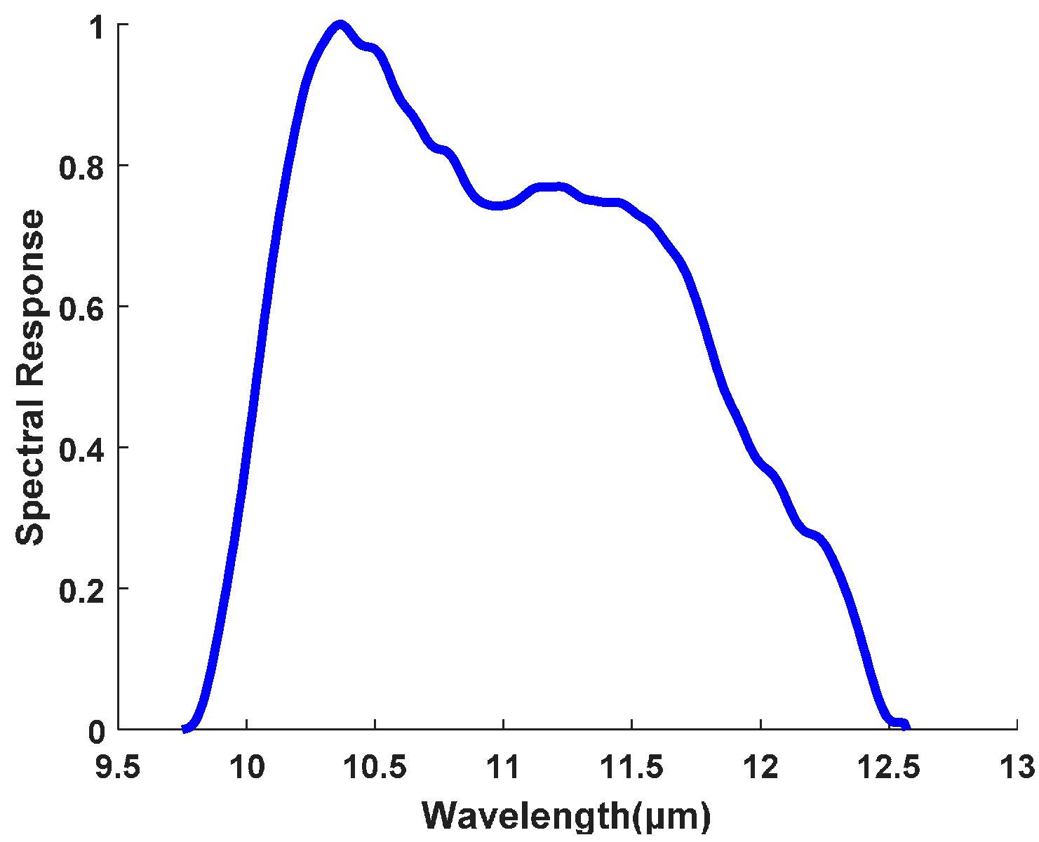
The land surface was divided into vegetated surfaces and bare soils to calculate their LSEs, respectively. Figure 3 shows the spectral response for band 5 of the FY-3C/MERSI. We can see that the MERSI has a broadband spectral range of 9.5–13 µm, which is inside the spectral range of GLASS BBE (8–13.5 µm). The study of Ren and Cheng [59] indicated that a linear relationship between MERSI emissivity and GLASS BBE existed for bare soils using the soil emissivity spectra in the ASTER spectral library. As the accuracy of GLASS BBE is better than 0.02 [60], the performance of this linear relationship is certainly better than the constant assumption or a linear function fitting of red reflectance adopted by the NDVI threshold and the VCM methods in predetermining LSE for LST estimation. Thus, the GLASS BBE was used to determine the LSE for LST estimation from the FY-3C/MERSI. The emissivity of the bare soils was estimated with the following equations:
where is the soil emissivity and is the GLASS BBE. The regression coefficients are determined by a total of 45 emissivity spectra from the ASTER spectral library, MODIS spectral library and the measured soil emissivity from Wang et al. [43].
Regarding the vegetated surfaces, we followed the method proposed by Cheng et al. [49], which can reflect the abundance of the vegetation and also has an accuracy of better than 0.005 over the fully covered vegetated surface. We used the 4Scattering by Arbitrary Inclined Leaves (4SAIL) model to construct a lookup table (LUT) of the LSE for vegetated surfaces. The variation ranges for three principal model inputs were set as follows: the leaf emissivity ranges from 0.935 to 0.995 and has an interval of 0.01; the soil emissivity varies from 0.71 to 0.99 and has an interval of 0.01; and the LAI ranges from 0 to 6.0 and has an interval of 0.5. After that, we can derive the emissivity of vegetated surfaces by interpolating the LUT using three inputs: leaf emissivity, soil emissivity, and LAI. Vegetated surfaces were identified using the NDVI calculated from MOD09GQ. LAI was extracted from the GLASS LAI product. Leaf emissivity was calculated from the measurements by Pandya et al. [61], Wang et al. [43], and the ASTER and MODIS spectral library for five composited vegetation land cover types based on MCD12Q1; these are shown in Table 1. The soil background emissivity underneath the vegetation canopy was derived from the mean GLASS BBE from month 10 of this year to month 4 of the following year. The land surface in this period is covered by soil rather than vegetation, and the emissivity in this period is the emissivity of the soil background for vegetated surfaces.
4. Results and Analysis
4.1. Coefficients for Atmospheric Correction
Values for and in Equation (9) can be derived after running the RTTOV, or they can be calculated from the precipitable water vapor through the following expression:
Different coefficients are obtained for each VZA when regressions of and are completed against and . To obtain a uniform angular dependent atmospheric correction expression, a linear function of is used [62], and the quadratic equation can be written as follows:
where S = , a1, a2, a3, b1, b2, b3, c1, c2 and c3 are the coefficients of the formula. The angular dependent atmospheric correction coefficients for FY-3C/MERSI are given in Table 2 and the coefficient of determination of 0.99 was obtained by fitting all data to Equation (12).
4.2. Evaluation with the In Situ LSE
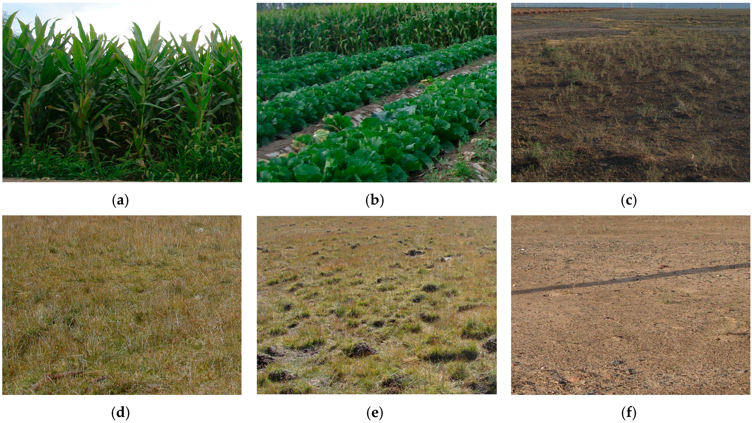
In this paper, the measured emissivities on 4 September 2014 or 5 September 2014 were selected to validate the estimated LSE on 4 September 2014. The emissivities were measured near the in situ sites by the 102F Portable Fourier Transform Infrared (FTIR) Spectrometer [63]. There are six measurements for the vegetation surfaces, namely, corn leaf, Chinese cabbage leaf, Alhagi sparsifolia, sparse vegetation, large cluster sparse vegetation, and one measurement for bare soil. The leaf emissivity of corn and Chinese cabbage were measured on 5 September 2014, the emissivities of other types were measured on 4 September 2014.
Table 3 summarizes the values of measured emissivity, estimated LSE and the bias between them for the different sites. Figure 4 shows the photos of measurement sites. Compared to the measured emissivity values, the LSE at the CJZ01, SSW02, SSW03 and GB02 sites were overestimated by 0.012, 0.025, 0.003 and 0.003, respectively; and LSE at CJZ02, GB01 and SSW01 sites were underestimated by 0.002, 0.016 and 0.015, respectively. What the spectrometer actually measured at the CJZ01 site is the emissivity of corn leaf, and so it is lower than the estimated LSE because the multi-scattering is not considered. The bias is very small at a relatively homogeneous site such as GB02. Regarding the sparsely vegetated surfaces, the spatial scaling effect is very strong because it is difficult to determine exactly what the spectrometer has seen in its narrow field of view. We should be very cautious when using the measured data in sparse vegetation. For example, the field of view of the spectrometer may be totally soil or vegetation canopy if the vegetation coverage is quite low. Figure 4c can also illustrate this phenomenon. The measured object is Alhagi sparsifolia, whose area ratio is quite low in the whole pixel, and so the estimated LSE of the whole pixel is close to the measured soil emissivity (Figure 4f). The larger bias that appears over GB01 and SSW02 is not difficult to understand. Assuming that the measured emissivity is accurate enough, the large bias between the measured emissivity and estimated LSE may come from the uncertainty of a new emissivity determination method or the spatial variability of field stations, both of which will be discussed in the following sections.
4.3. Sensitivity Analysis of Emissivity
To analyze the effects of leaf emissivity, soil emissivity and LAI on the estimated LSE over vegetated surfaces, we adhered to the following rules to conduct the simulation: (1) the leaf emissivity ranges from 0.92 to 0.98 with an interval of 0.02, the LAI ranges from 0.1 to 6.0 with an interval of 0.5 from 0.5 to 6.0, and the soil emissivity was set to 0.96; (2) the soil emissivity ranges from 0.90 to 0.98 with an interval of 0.02, the LAI ranges from 0.1 to 6.0 with an interval of 0.5 from 0.5 to 6.0, and the leaf emissivity was set to 0.96. Figure 5 shows the emissivity calculated from the 4SAIL model. When the LAI values change from 0.1 to 2.0, the variation of soil emissivity has more influence on the estimated LSE than the variation of the leaf emissivity. In this range, when the leaf emissivity changes from 0.92 to 0.98, the difference between the maximum and minimum estimated LSE changed from 0.033 to 0.046, but when the soil emissivity changed from 0.90 to 0.98, the difference between the maximum and minimum estimated LSE changed from 0.075 to 0.007. This indicated that the soil emissivity might cause great errors to the estimated LSE of the vegetated surface when the LAI is less than 2.0. The emissivity shows little change when the LAI is greater than 3.0, when the leaf emissivity changes from 0.92 to 0.98, the emissivity remains from 0.978 to 0.994, no matter how the soil emissivity and LAI change. The emissivity shows little change when the LAI is greater than 3.0, when the soil emissivity changes from 0.90 to 0.98 and the leaf emissivity is equal to 0.96, the emissivity remains 0.989, no matter how much the LAI changes.
We also analyzed the stability of the soil background emissivity underneath the vegetation canopy and the applicability of the regression formula over bare soils. First, we plot the BBE of each eight-day period from 2001 to 2014 for different stations, as shown in Figure 6. As described in Section 3.3, the emissivity from month 10 of this year to month 4 of next year is the emissivity of the soil background for vegetated surfaces. We can infer from this that the soil background emissivity underneath the vegetation canopy is stable, based on Figure 6. According to the validation using four field trials by Cheng et al. [39], the accuracy of the GLASS BBE of bare soil is 0.016, and so the mean soil emissivity can be used to represent the soil background emissivity underneath the vegetation canopy. Second, using only one formula to regress the relationship between the GLASS BBE and estimated LSE may introduce some errors. The BBE variation is various for the different soil types, different seasons and different areas [49]. This trend is also obvious in Figure 6, as the BBE are slightly different at the various stations. Because of this, we chose soil and sand samples from the spectral library to calculate the regression coefficient between the GLASS BBE and estimated LSE, respectively. The regression results from soil and sand samples are obviously different, so it is noteworthy when using the regression formula. If we used the regression formula for soil samples to calculate the LSE of the sand surface, it may be inaccurate.
4.4. Validation of Retrieved LST from FY-3C/MERSI with In Situ LST
Both the radiative transfer equation algorithm and the generalized single-channel algorithm were used for estimating the LST from the FY-3C/MERSI images acquired in 2014. Figure 7 shows the statistical results between the estimated LST from the RTE algorithm or the GSC algorithm and the in situ LST. The results derived from the RTE algorithm, using the LSE calculated by the new emissivity scheme, was denoted as RTE1. The NDVI threshold method developed by Sobrino et al. [33] was also used to retrieve the LST by the RTE algorithm. The results were called RTE2 accordingly. The results derived from the GSC algorithm, which the LSE calculated by new scheme, was denoted as GSC1, whereas the result derived from the GSC algorithm using the LSE calculated by the NDVI threshold method was denoted as GSC2. Note that the LST of the GSC algorithm on 17 July 2014 was empty due to a lack of atmospheric water vapor data.
From Figure 7, we can see that there is a high correlation between the estimated LST and the in situ LSTs for both the RTE algorithm and the GSC algorithm. The bias and STD (RMSE) of the RTE algorithm with the LSE derived from the new scheme are −0.92 K and 1.53 K (1.77 K). The bias and STD (RMSE) of the RTE algorithm using the LSE calculated by the NDVI threshold method are −0.82 K and 1.77 K (1.94 K). The bias and STD (RMSE) of the GSC algorithm with the LSE derived from the new LSE scheme are 0.45 K and 1.85 K (1.89 K). The bias and STD (RMSE) of the GSC algorithm using the LSE calculated by the NDVI threshold method are 0.98 K and 1.94 K (2.16 K). The validation results showed that the estimated LSTs are obviously underestimated at most stations for the two RTE algorithms, while most of the LSTs derived from the GSC algorithm was overestimated. Overall, we can conclude that the new LSE scheme can achieve a higher precision of LST determination.
Comparing the LSE derived by the NDVI threshold method with the LSE derived by the new scheme, the two methods have nearly similar LSTs, because the soil emissivity used here is the same as the new scheme, rather than the constant assumption adopted by the original NDVI threshold. According to the MODIS precipitable water product (MOD05), most of the total water vapor content of the validation stations in 2014 was less than 2.0 g/cm2, and so the RTE and GSC algorithms all have obtained a high level of accuracy. The results are consistent with the study by Jiménez-Muñoz et al. [31], who claimed that the GSC algorithm has a high accuracy in a low water vapor content area. Although a high precision of the LST can be achieved with the LSE determined by the new scheme, we should be very cautious when using the atmospheric profiles for atmospheric correction. When the surroundings of study area were covered by clouds, the LST of the RTE algorithm is underestimated, e.g., JCHM station on 24 August 2014.
5. Discussion
5.1. Comparison with LST Derived from ASTER Emissivity Product
In this section, we used the LSE calculated from the ASTER Surface Emissivity product (AST_05) to evaluate the accuracy of the LSE estimated by the new scheme, as well as the estimated LSTs. The AST_05 is an on-demand product generated using the Temperature/Emissivity Separation (TES) algorithm [12] and combined with the Water Vapor Scaling (WVS) atmospheric correction method [55] for the five thermal infrared (TIR) 90 m resolution bands. The study by Hully et al. [64] indicated that the accuracies in retrieving the spectral emissivity for ASTER were below 0.016. The AST_05 product on 23 July 2014 was used to evaluate the emissivity determined by the new scheme.
First, the FY-3C/MERSI LSE can be calculated from the linear transformation formula, as shown in Equation (13). We adopted the least-squares fitting method to establish the transformation formula, using the 251-emissivity spectra in the ASTER spectral library and the spectral response function of the ASTER band 13, 14 and FY-3C/MERSI.
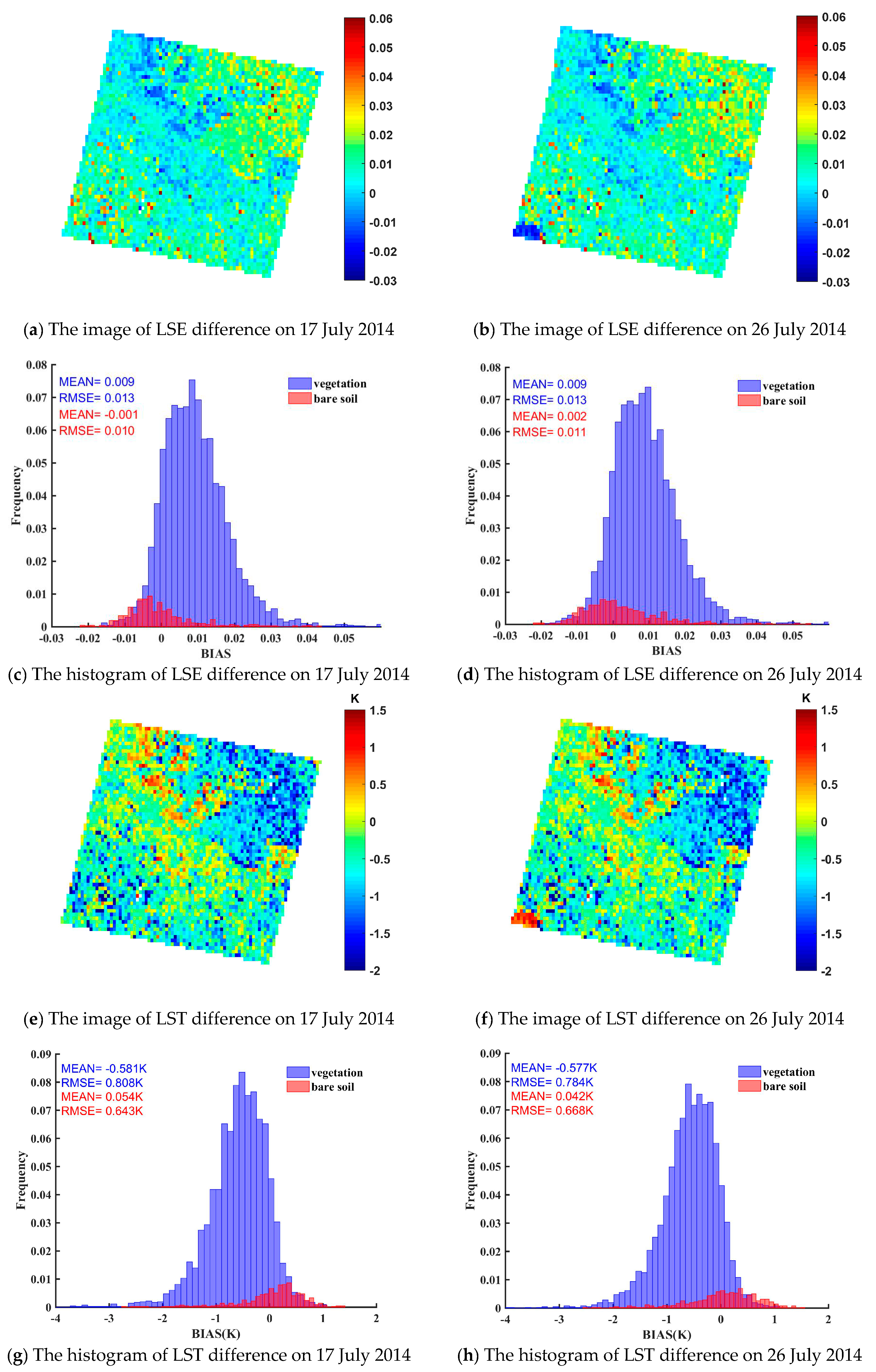
where LSEaster, and are the land surface emissivity of the FY-3C/MERSI and ASTER channels 13 and 14, respectively. Then, we compared the estimated LSE on 17 and 26 July 2014 to the LSE calculated from AST_05 on 23 July 2014, assuming that the land surface emissivity of the study area is stable during a short time. Figure 8 shows the images of the LSE difference on 17 and 26 July 2014 and the corresponding images of the LST difference. The LSE difference was calculated using the LSE estimated from the scheme presented in this paper (LSEmersi) minus the LSE estimated from the AST_05 product (LSEaster). The LSTs were derived from the RTE algorithm. The histogram of the LSE difference on 17 and 26 July 2014 and the corresponding histogram of the LST difference (LSTmersi − LSTaster) are also provided.
The average bias of the LSE difference over vegetated surfaces on 17 July 2014 is 0.009 and the RMSE is 0.013. The average bias and RMSE of the LSE difference over the vegetated surface on 26 July 2014 are the same as the values on 17 July 2014. The new scheme provides accurate values over bare soil surface on 17 July 2014 and 26 July 2014, with an average bias of less than 0.002 and a RMSE of less than 0.011, respectively. The LSE estimated from the new scheme over the vegetated surface on 17 July 2014 and on 26 July 2014 have been overestimated by 0.01, when compared with the LSE estimated from the AST_05 product. This result is consistent with the experiments of Gillespie et al. [65] and the research of Jiménez-Muñoz et al. [66]. They found that the TES algorithm has larger uncertainties over low spectral contrast surfaces, such as vegetation, and it provides accurate values for soil and rocks [49].
The average bias of the LST difference over vegetated surfaces on 17 July 2014 is −0.581 K and the RMSE is 0.808 K. The average bias and RMSE of the LST difference over vegetated surfaces on 26 July 2014 are −0.577 K and 0.784 K, respectively. The new scheme provides accurate values over the bare soil surfaces on 17 July 2014 and 26 July 2014, with an average bias of less than 0.06 K and RMSE less than 0.7 K, respectively. The statistical results show that the LST bias over the vegetated and bare soil surfaces have small statistical errors, most of the absolute bias values are within 2 K. Table 4 shows the results of the LSE estimated from AST_05 and that determined by the new scheme on 17 and 26 July 2014, as well as the corresponding LST at the validation stations. The LSEs of the GB and HZZ sites provided accurate values on 17 and 26 July 2014, with biases of less than 0.003 and the biases of the corresponding LSTs are within 0.3 K. Compared with the LSEs estimated from AST_05, the LSEs of the SSW site are overestimated by 0.01 and 0.013, respectively, and the LSTs are underestimated by 0.71 K and 0.87 K, respectively. The LSTs of the SD and CJZ sites are all within 2 K with in situ measured LSTs. From the above analyses, we can conclude that the LSE determined by the new scheme is acceptable over a bare soil surface compared with the LSE directly calculated from the AST_05 product. Therefore, a high precision of the LST can be achieved from the RTE algorithm with the LSE determined by the new scheme.
5.2. Effects of Spatial Scale on the LST and LSE Evaluation
The LST validation sites must be homogeneous from the point scale to several kilometers [67,68]. The spatial variability of the validation stations has large effects on the validation results. To analyze the spatial variability of the six validation stations, we extracted the LSE or LST of the 3 × 3 (270 m), 5 × 5 (450 m), 7 × 7 (630 m), 9 × 9 (810 m), and 11 × 11 (990 m) pixels centered on each validation station from the twenty scenes of the ASTER LSE or LST products, respectively. The standard deviation of the different window sizes calculated from the twenty scenes of the ASTER LST or ASTER LSE products reflects the spatial variability of the validation stations. The average standard deviations of the different window sizes at the six stations are shown in Table 5. The average standard deviation of the ASTER LSE at the six stations changes little or remains the same with the various window sizes, with a range from 0.003 to 0.006. The average standard deviation of the ASTER LSE over the bare soil surface, e.g., HZZ and JCHM station changes are smaller than the vegetation surface, e.g., CJZ and SD stations. The average standard deviation of the ASTER LST at the six stations changes variously with the different window sizes. The HZZ, JCHM and GB stations show the lower standard deviation at all window sizes, with a range from 0.34 K to 0.89 K. The standard deviation of the SD and CJZ sites were higher than 1.0 K, except the 3 × 3 window size, which had a range from 1.04 K to 1.98 K. It appears to be that the two vegetation sites have higher heterogeneity than other sites.
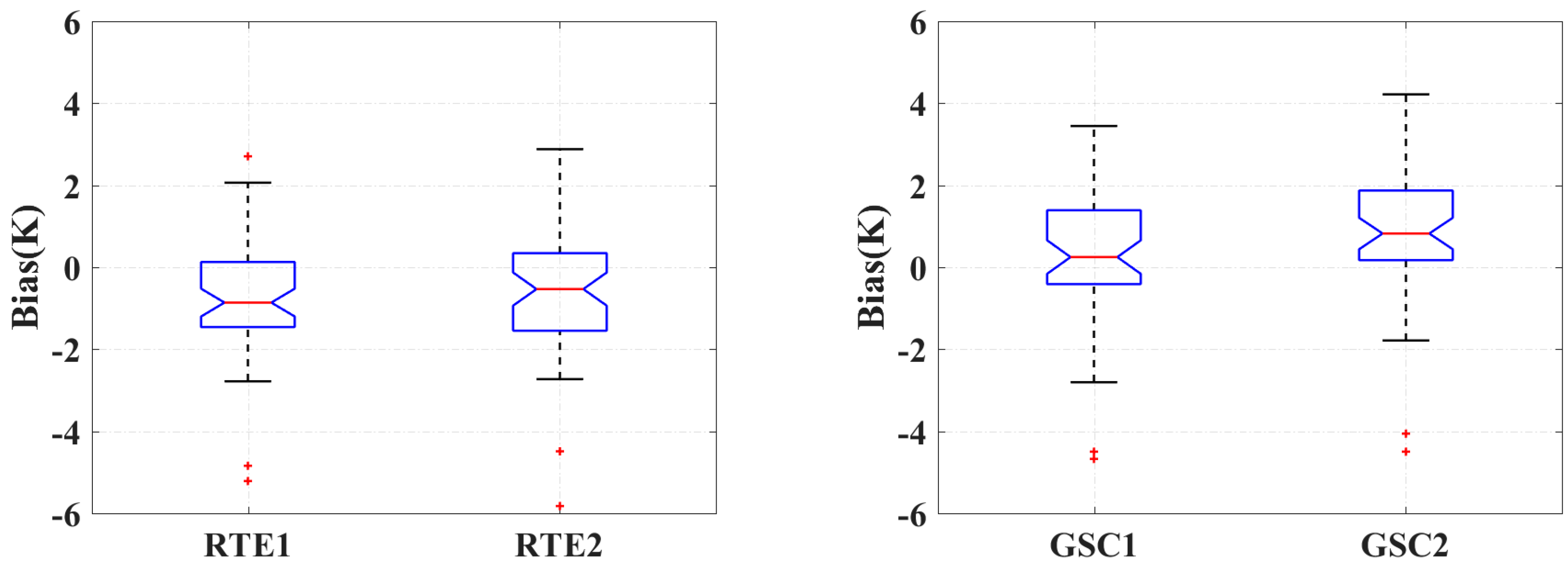
To illustrate the heterogeneous surface’s effects on the estimated LST, we estimated the land surface temperature using the 250 m FY-3C/MERSI data. The GLASS BBE and GLASS LAI products were resized to a 250 m resolution based on the nearest neighbor interpolation model. Figure 9 shows the boxplots between the estimated LSTs from the RTE algorithm (left) or the GSC algorithm (right) at a 250 m resolution and ground LSTs. The trend is similar to the results of the 1000 m spatial resolution. The estimated LSTs are obviously underestimated in the RTE algorithm and most of the LSTs derived from the GSC algorithm were larger than the in situ LSTs.
Compared with the results of the two algorithms at 1000 m resolution, the deviation of the two algorithms at 250 m resolution has improved to a certain extent. The bias of the RTE algorithm has changed from −0.92 K to −0.73 K for RTE1 and from −0.82 K to −0.53 K for RTE2. The bias of the GSC algorithm has changed from 0.45 K to 0.23 K for GSC1 and from 0.98 K to 0.87 K for GSC2. In addition, the STD (RMSE) of the RTE and GSC algorithms are all less than 1.76 K (1.95 K). From the above analyses, we can conclude that the two LST algorithms with the LSE derived from the new scheme are all suitable for estimating land surface temperatures. The estimated LSTs with the new LSE scheme have a higher precision than the estimated LST with the NDVI threshold method. Although the scaling effect on the ASTER LST is significant, the heterogeneous surface has little effect on the estimated LST for the coarser spatial resolution (250 m and 1000 m).
6. Conclusions
In this study, we proposed a new scheme to predetermine the LSE for estimating LST from the FY-3C/MERSI with only one thermal infrared channel. The new scheme first divides the land surface into bare soils and vegetated surfaces, then takes advantage of the 4SAIL model’s ability to derive the land surface emissivity for vegetated surfaces and establishes the linear relationship between the GLASS BBE and the land surface emissivity of the FY-3C/MERSI data for bare soil surfaces. After determining the LSE, the LST was retrieved by using the RTE and GSC algorithms.
The LSE derived by the new scheme was validated by the field measurements collected at seven stations during the HiWATER experiment. The mean difference between the derived LSE and field-measured LSE is approximately 0.002. When the LSE determined by the new scheme was used for the LST retrieval from the FY-3C/MERSI data using the RTE and GSC algorithms, an acceptable accuracy was achieved, i.e., at 1000 m resolution, the absolute bias of the two algorithms were less than 1 K, and the STD (RMSE) values were all less than 1.95 K (2.2 K). At 250 m resolution, the absolute bias, STD and RMSE of the two algorithms were all less than 0.87 K, 1.76 K and 1.95 K, respectively. Compared to the LST derived by the same algorithm but with the commonly used NDVI threshold method, the new land surface emissivity scheme can achieve better results. Additionally, the new scheme was evaluated by the ASTER emissivity product. The new scheme can provide an accurate LSE estimate, with an average bias of less than 0.009 and RMSE of less than 0.013. Both the ASTER LSE and LSE determined by the new scheme were used to retrieve the LST from the FY-3C/MERSI data, and good agreement was obtained. The average bias and RMSE of the corresponding LST differences are −0.6 K and 0.8 K, respectively. Regarding the validation and evaluation results, we can conclude that the new emissivity scheme can be used to improve the accuracy of the LSE and further the LST for sensors with a broad spectral range such as the FY-3C/MERSI.
Acknowledgments
The ground data used in this study is provided by Cold and Arid Regions Science Data Center at Lanzhou (http://westdc.westgis.ac.cn). The GLASS BBE and LAI products are downloaded from GLCF (ftp://ftp.glcf.umd.edu/glcf/GLASS/). The MODIS products are downloaded from NASA (https://search.earthdata.nasa.gov/). This work was partly supported by the National Natural Science Foundation of China via grant 41771365, the National Key Research and Development Program of China via grant 2016YFA0600101, and the National Natural Science Foundation of China via grant 41371323.
Author Contributions
Jie Cheng conceived and designed the algorithm; Xiangchen Meng performed the algorithm, analyzed the data and wrote the paper. All authors participated in the editing of the paper.
Conflicts of Interest
The authors declare no conflict of interest.
References
- Wan, Z.; Dozier, J. A generalized split-window algorithm for retrieving land-surface temperature from space. IEEE Trans. Geosci. Remote Sens. 1996, 34, 892–905. [Google Scholar]
- Mannstein, H. Surface Energy Budget, Surface Temperature and Thermal Inertia. In Remote Sensing Applications in Meteorology and Climatology; Vaughan, R.A., Ed.; Springer Netherlands: Dordrecht, The Netherlands, 1987; pp. 391–410. [Google Scholar]
- Valor, E.; Caselles, V. Mapping land surface emissivity from NDVI: Application to european, African, and South American areas. Remote Sens. Environ. 1996, 57, 167–184. [Google Scholar] [CrossRef]
- Cheng, J.; Liang, S.; Wang, J.; Li, X. A stepwise refining algorithm of temperature and emissivity separation for hyperspectral thermal infrared data. IEEE Trans. Geosci. Remote Sens. 2010, 48, 1588–1597. [Google Scholar] [CrossRef]
- Li, Z.-L.; Wu, H.; Wang, N.; Qiu, S.; Sobrino, J.A.; Wan, Z.-M.; Tang, B.-H.; Yan, G.-J. Land surface emissivity retrieval from satellite data. Int. J. Remote Sens. 2013, 34, 3084–3127. [Google Scholar]
- Qin, Z.; Karnieli, A.; Berliner, P. A mono-window algorithm for retrieving land surface temperature from landsat tm data and its application to the Israel-Egypt border region. Int. J. Remote Sens. 2001, 22, 3719–3746. [Google Scholar]
- Jiménez-Muñoz, J.C. A generalized single-channel method for retrieving land surface temperature from remote sensing data. J. Geophys. Res. Atmos. 2003, 108. [Google Scholar] [CrossRef]
- Ellicott, E.; Vermote, E.; Petitcolin, F.; Hook, S.J. Validation of a new parametric model for atmospheric correction of thermal infrared data. IEEE Trans. Geosci. Remote Sens. 2008, 47, 295–311. [Google Scholar] [CrossRef]
- Becker, F.; Li, Z.L. Towards a local split window method over land surfaces. Int. J. Remote Sens. 1990, 11, 369–393. [Google Scholar] [CrossRef]
- Yu, Y.; Privette, J.L.; Pinheiro, A.C. Evaluation of split-window land surface temperature algorithms for generating climate data records. IEEE Trans. Geosci. Remote Sens. 2008, 46, 179–192. [Google Scholar] [CrossRef]
- Yunyue, Y.; Tarpley, D.; Privette, J.L.; Goldberg, M.D.; Rama Varma Raja, M.K.; Vinnikov, K.Y.; Hui, X. Developing algorithm for operational GOES-R land surface temperature product. IEEE Trans. Geosci. Remote Sens. 2009, 47, 936–951. [Google Scholar] [CrossRef]
- Gillespie, A.; Rokugawa, S.; Matsunaga, T.; Cothern, J.S.; Hook, S.; Kahle, A.B. A temperature and emissivity separation algorithm for advanced spaceborne thermal emission and reflection radiometer (ASTER) images. IEEE Trans. Geosci. Remote Sens. 1998, 36, 1113–1126. [Google Scholar] [CrossRef]
- Masiello, G.; Serio, C.; De Feis, I.; Amoroso, M.; Venafra, S.; Trigo, I.F.; Watts, P. Kalman filter physical retrieval of surface emissivity and temperature from geostationary infrared radiances. Atmos. Meas. Tech. 2013, 6, 3613–3634. [Google Scholar] [CrossRef]
- Coll, C.; Caselles, V.; Valor, E.; Niclòs, R.; Sánchez, J.M.; Galve, J.M.; Mira, M. Temperature and emissivity separation from ASTER data for low spectral contrast surfaces. Remote Sens. Environ. 2007, 110, 162–175. [Google Scholar] [CrossRef]
- Sobrino, J.; Jimenezmunoz, J.; Balick, L.; Gillespie, A.; Sabol, D.; Gustafson, W. Accuracy of ASTER level-2 thermal-infrared standard products of an agricultural area in Spain. Remote Sens. Environ. 2007, 106, 146–153. [Google Scholar] [CrossRef]
- Wan, Z. New refinements and validation of the collection-6 modis land-surface temperature/emissivity product. Remote Sens. Environ. 2014, 140, 36–45. [Google Scholar] [CrossRef]
- Liu, Y.; Yu, Y.; Yu, P.; Göttsche, F.; Trigo, I. Quality assessment of S-NPP VIIRS land surface temperature product. Remote Sens. 2015, 7, 12215–12241. [Google Scholar] [CrossRef]
- Sun, D.; Pinker, R.T. Estimation of land surface temperature from a geostationary operational environmental satellite (GOES-8). J. Geophys. Res. Atmos. 2003, 108. [Google Scholar] [CrossRef]
- Sun, D.; Yu, Y. Land Surface Temperature (LST) Retrieval from Goes Satellite Observations. In Satellite-based Applications on Climate Change; Qu, J., Powell, A., Sivakumar, M., Eds.; Springer Netherlands: Dordrecht, The Netherlands, 2013; pp. 289–334. [Google Scholar]
- Masiello, G.; Serio, C.; Venafra, S.; Liuzzi, G.; Göttsche, F.; Trigo, I.F.; Watts, P. Kalman filter physical retrieval of surface emissivity and temperature from seviri infrared channels: A validation and intercomparison study. Atmos. Meas. Tech. 2015, 8, 2981–2997. [Google Scholar] [CrossRef]
- Weng, Q.; Lu, D.; Schubring, J. Estimation of land surface temperature-vegetation abundance relationship for urban heat island studies. Remote Sens. Environ. 2004, 89, 467–483. [Google Scholar] [CrossRef]
- Imhoff, M.L.; Zhang, P.; Wolfe, R.E.; Bounoua, L. Remote sensing of the urban heat island effect across biomes in the continental USA. Remote Sens. Environ. 2010, 114, 504–513. [Google Scholar] [CrossRef]
- Fee, D.; Matoza, R.S. An overview of volcano infrasound: From hawaiian to plinian, local to global. J. Volcanol. Geotherm. Res. 2013, 249, 123–139. [Google Scholar] [CrossRef]
- Diker, C.; Ulusoy, I. Monitoring Thermal Activity of Eastern Anatolian Volcanoes Using Modis Images. In Proceedings of the European Geosciences Union General Assembly, Vienna, Austria, 27 April–2 May 2014; pp. 375–381. [Google Scholar]
- Ulusoy, İ. Temporal monitoring of radiative heat flux from the craters of tendürek volcano (East Anatolia, Turkey) using ASTER satellite imagery. In Proceedings of the European Geosciences Union General Assembly, Vienna, Austria, 27 April–2 May 2014. [Google Scholar]
- Guangmeng, Q.; Mei, Z. Using MODIS land surface temperature to evaluate forest fire risk of Northeast China. IEEE Geosci. Remote Sens. Lett. 2004, 1, 98–100. [Google Scholar] [CrossRef]
- ManzoDelgado, L.; SánchezColón, S.; Álvarez, R. Assessment of seasonal forest fire risk using NOAA-AVHRR: A case study in central mexico. Int. J. Remote Sens. 2009, 30, 4991–5013. [Google Scholar] [CrossRef]
- Meng, X.; Li, H.; Du, Y.; Liu, Q.; Zhu, J.; Sun, L. Retrieving land surface temperature from landsat 8 TIRS data using RTTOV and ASTER GED. In Proceedings of the Geoscience and Remote Sensing Symposium, Beijing, China, 10–15 July 2016; pp. 4302–4305. [Google Scholar]
- Yu, X.; Guo, X.; Wu, Z. Land surface temperature retrieval from landsat 8 TIRS—Comparison between radiative transfer equation-based method, split window algorithm and single channel method. Remote Sens. 2014, 6, 9829–9852. [Google Scholar] [CrossRef]
- Windahl, E.; Beurs, K.D. An intercomparison of landsat land surface temperature retrieval methods under variable atmospheric conditions using in situ skin temperature. Int. J. Appl. Earth Obs. Geoinf. 2016, 51, 11–27. [Google Scholar] [CrossRef]
- Jimenez-Munoz, J.C.; Cristobal, J.; Sobrino, J.A.; Soria, G.; Ninyerola, M.; Pons, X.; Pons, X. Revision of the single-channel algorithm for land surface temperature retrieval from landsat thermal-infrared data. IEEE Trans. Geosci. Remote Sens. 2009, 47, 339–349. [Google Scholar] [CrossRef]
- Zhou, J.; Zhan, W.; Hu, D.; Zhao, X. Improvement of mono-window algorithm for retrieving land surface temperature from HJ-1B satellite data. Chin. Geogr. Sci. 2010, 20, 123–131. [Google Scholar] [CrossRef]
- Sobrino, J.A.; Raissouni, N.; Li, Z.L. A comparative study of land surface emissivity retrieval from NOAA data. Remote Sens. Environ. 2001, 75, 256–266. [Google Scholar] [CrossRef]
- Snyder, W.C.; Wan, Z.; Zhang, Y.; Feng, Y.Z. Classification-based emissivity for land surface temperature measurement from space. Int. J. Remote Sens. 1998, 19, 2753–2774. [Google Scholar] [CrossRef]
- Hulley, G.; Veraverbeke, S.; Hook, S. Thermal-based techniques for land cover change detection using a new dynamic MODIS multispectral emissivity product (MOD21). Remote Sens. Environ. 2014, 140, 755–765. [Google Scholar] [CrossRef]
- Li, H.; Sun, D.; Yu, Y.; Wang, H.; Liu, Y.; Liu, Q.; Du, Y.; Wang, H.; Cao, B. Evaluation of the VIIRS and MODIS lst products in an arid area of Northwest China. Remote Sens. Environ. 2014, 142, 111–121. [Google Scholar] [CrossRef]
- Liang, S.; Zhao, X.; Liu, S.; Yuan, W.; Cheng, X.; Xiao, Z.; Zhang, X.; Liu, Q.; Cheng, J.; Tang, H.; et al. A long-term global land surface satellite (GLASS) data-set for environmental studies. Int. J. Digit. Earth 2013, 6, 5–33. [Google Scholar] [CrossRef]
- Cheng, J.; Liang, S. Estimating global land surface broadband thermal-infrared emissivity from the advanced very high resolution radiometer optical data. Int. J. Digit. Earth 2013, 6, 34–49. [Google Scholar] [CrossRef]
- Cheng, J.; Liang, S. Estimating the broadband longwave emissivity of global bare soil from the MODIS shortwave albedo product. J. Geophys. Res. Atmos. 2014, 119, 614–634. [Google Scholar] [CrossRef]
- Xiao, Z.; Liang, S.; Wang, J.; Chen, P.; Yin, X.; Zhang, L.; Song, J. Use of general regression neural networks for generating the glass leaf area index product from time-series MODIS surface reflectance. IEEE Trans. Geosci. Remote Sens. 2013, 52, 209–223. [Google Scholar] [CrossRef]
- Xu, Z.; Liu, S.; Li, X.; Shi, S.; Wang, J.; Zhu, Z.; Xu, T.; Wang, W.; Ma, M. Intercomparison of surface energy flux measurement systems used during the HIWATER-MUSOEXE. J. Geophys. Res. Atmos. 2013, 118, 13140–13157. [Google Scholar] [CrossRef]
- Li, X.; Cheng, G.; Liu, S.; Xiao, Q.; Ma, M.; Jin, R.; Che, T.; Liu, Q.; Wang, W.; Qi, Y.; et al. Heihe watershed allied telemetry experimental research (HIWATER): Scientific objectives and experimental design. Bull. Am. Meteorol. Soc. 2013, 94, 1145–1160. [Google Scholar] [CrossRef]
- Wang Heshun, L.H.; Cao, B.; Du, Y.; Xiao, Q.; Liu, Q. HIWATER: Dataset of Thermal Infrared Spectrum Observed by BOMEM MR304 in the Middle Reaches of the Heihe River Basin; Institute of Remote Sensing Applications, Chinese Academy of Sciences: Beijing, China, 2012. [Google Scholar]
- Liu, S.M.; Xu, Z.W.; Wang, W.Z.; Jia, Z.Z.; Zhu, M.J.; Bai, J.; Wang, J.M. A comparison of eddy-covariance and large aperture scintillometer measurements with respect to the energy balance closure problem. Hydrol. Earth Syst. Sci. 2011, 15, 1291–1306. [Google Scholar] [CrossRef]
- Tan Junlei, M.M. HIWATER: Dataset of Infrared Temperature in Zhanye Airport Desert; Cold and Arid Regions Environmental and Engineering Research Institute, Chinese Academy of Sciences: Beijing, China, 2012. [Google Scholar]
- Ingram, P.M.; Muse, A.H. Sensitivity of iterative spectrally smooth temperature/emissivity separation to algorithmic assumptions and measurement noise. IEEE Trans. Geosci. Remote Sens. 2001, 39, 2158–2167. [Google Scholar] [CrossRef]
- Cheng, J.; Liang, S.; Yao, Y.; Ren, B.; Shi, L.; Liu, H. A comparative study of three land surface broadband emissivity datasets from satellite data. Remote Sens. 2013, 6, 111–134. [Google Scholar] [CrossRef]
- Jimenez-Munoz, J.C.; Sobrino, J.A. Feasibility of retrieving land-surface temperature from ASTER TIR bands using two-channel algorithms: A case study of agricultural areas. IEEE Geosci. Remote Sens. Lett. 2007, 4, 60–64. [Google Scholar] [CrossRef]
- Cheng, J.; Liang, S.; Verhoef, W.; Shi, L.; Liu, Q. Estimating the hemispherical broadband longwave emissivity of global vegetated surfaces using a radiative transfer model. IEEE Trans. Geosci. Remote Sens. 2016, 54, 905–917. [Google Scholar] [CrossRef]
- Barsi, J.A.; Butler, J.J.; Schott, J.R.; Palluconi, F.D.; Hook, S.J. Validation of a web-based atmospheric correction tool for single thermal band instruments. In Proceedings of the Optics and Photonics, San Diego, CA, USA, 31 July–4 August 2005; Volume 5882, pp. 136–142. [Google Scholar]
- Li, H.; Liu, Q.; Du, Y.; Jiang, J.; Wang, H. Evaluation of the NCEP and MODIS atmospheric products for single channel land surface temperature retrieval with ground measurements: A case study of HJ-1B IRS data. IEEE J. Sel. Top. Appl. Earth Obs. Remote Sens. 2013, 6, 1399–1408. [Google Scholar] [CrossRef]
- Cook, M.; Schott, J.; Mandel, J.; Raqueno, N. Development of an operational calibration methodology for the landsat thermal data archive and initial testing of the atmospheric compensation component of a land surface temperature (LST) product from the archive. Remote Sens. 2014, 6, 11244–11266. [Google Scholar] [CrossRef]
- Rivalland, V.; Tardy, B.; Huc, M.; Hagolle, O.; Marcq, S.; Boulet, G. A useful tool for atmospheric correction and surface temperature estimation of landsat infrared thermal data. In Proceedings of the European Geosciences Union General Assembly, Vienna, Austria, 17–22 April 2016; Volume 8, p. 696. [Google Scholar]
- Matricardi, M.; Chevallier, F.; Kelly, G.; Thépaut, J.N. An improved general fast radiative transfer model for the assimilation of radiance observations. Q. J. R. Meteorol. Soc. 2010, 130, 153–173. [Google Scholar] [CrossRef]
- Tonooka, H. Accurate atmospheric correction of ASTER thermal infrared imagery using the WVS method. IEEE Trans. Geosci. Remote Sens. 2005, 43, 2778–2792. [Google Scholar] [CrossRef]
- Jiang, G.M.; Zhou, W.; Liu, R. Development of split-window algorithm for land surface temperature estimation from the VIRR/FY-3A measurements. IEEE Geosci. Remote Sens. Lett. 2013, 10, 952–956. [Google Scholar] [CrossRef]
- Borbas, E.E.; Seemann, S.W.; Huang, H.L.; Li, J.; Menzel, P.W. Global profile training database for satellite regression retrievals with estimates of skin temperature and emissivity. In Proceedings of the International TOVS Study Conference, Beijing, China, 25–31 May 2005. [Google Scholar]
- Galve, J.M.; Coll, C.; Caselles, V.; Valor, E. An atmospheric radiosounding database for generating land surface temperature algorithms. IEEE Trans. Geosci. Remote Sens. 2008, 46, 1547–1557. [Google Scholar] [CrossRef]
- Ren, B.; Cheng, J. Land Surface Temperature Retrieval Algorithm of Single Channel for FY-3A/MERSI; Beijing Normal University: Beijing, China, 2015. [Google Scholar]
- Dong, L.X.; Hu, J.Y.; Tang, S.H.; Min, M. Field validation of glass land surface broadband emissivity database using pseudo-invariant sand dunes sites in Northern China. Int. J. Digit. Earth 2013, 6, 96–112. [Google Scholar] [CrossRef]
- Pandya, M.R.; Shah, D.B.; Trivedi, H.J.; Lunagaria, M.M.; Pandey, V.; Panigrahy, S.; Parihar, J.S. Field measurements of plant emissivity spectra: An experimental study on remote sensing of vegetation in the thermal infrared region. J. Indian Soc. Remote Sens. 2013, 41, 787–796. [Google Scholar] [CrossRef]
- Niclòs, R.; Caselles, V.; Coll, C.; Valor, E. Determination of sea surface temperature at large observation angles using an angular and emissivity-dependent split-window equation. Remote Sens. Environ. 2007, 111, 107–121. [Google Scholar] [CrossRef]
- Yu Wenping, M.M.; Ren, Z.; Tan, J.; Li, Y.; Wang, H. HIWATER: Dataset of Emissivity in the Heihe River Basin; Cold and Arid Regions Science Data Center at Lanzhou: Lanzhou, China, 2013. [Google Scholar]
- Hulley, G.C.; Hughes, C.G.; Hook, S.J. Quantifying uncertainties in land surface temperature and emissivity retrievals from ASTER and MODIS thermal infrared data. J. Geophys. Res. Atmos. 2012, 117. [Google Scholar] [CrossRef]
- Guillevic, P.C.; Privette, J.L.; Coudert, B.; Palecki, M.A.; Demarty, J.; Ottlé, C.; Augustine, J.A. Land surface temperature product validation using NOAA’S surface climate observation networks—Scaling methodology for the visible infrared imager radiometer suite (VIIRS). Remote Sens. Environ. 2012, 124, 282–298. [Google Scholar] [CrossRef]
- Jiménez-Muñoz, J.C.; Sobrino, J.A.; Gillespie, A.; Sabol, D.; Gustafson, W.T. Improved land surface emissivities over agricultural areas using ASTER NDVI. Remote Sens. Environ. 2006, 103, 474–487. [Google Scholar] [CrossRef]
- Coll, C.; Valor, E.; Galve, J.M.; Mira, M.; Bisquert, M.; García-Santos, V.; Caselles, E.; Caselles, V. Long-term accuracy assessment of land surface temperatures derived from the advanced along-track scanning radiometer. Remote Sens. Environ. 2012, 116, 211–225. [Google Scholar] [CrossRef]
- Cheng, J.; Liang, S.; Dong, L.; Ren, B.; Shi, L. Validation of the moderate-resolution imaging spectrometer (MODIS) land surface emissivity products over the taklimakan desert. J. Appl. Remote Sens. 2014, 8. [Google Scholar] [CrossRef]
Figure 1.
Spatial distribution of the six in situ sites. (The base map is from HJ-1 CCD false color composite image and the RGB components are channels 4, 3 and 2, respectively).
Figure 1.
Spatial distribution of the six in situ sites. (The base map is from HJ-1 CCD false color composite image and the RGB components are channels 4, 3 and 2, respectively).
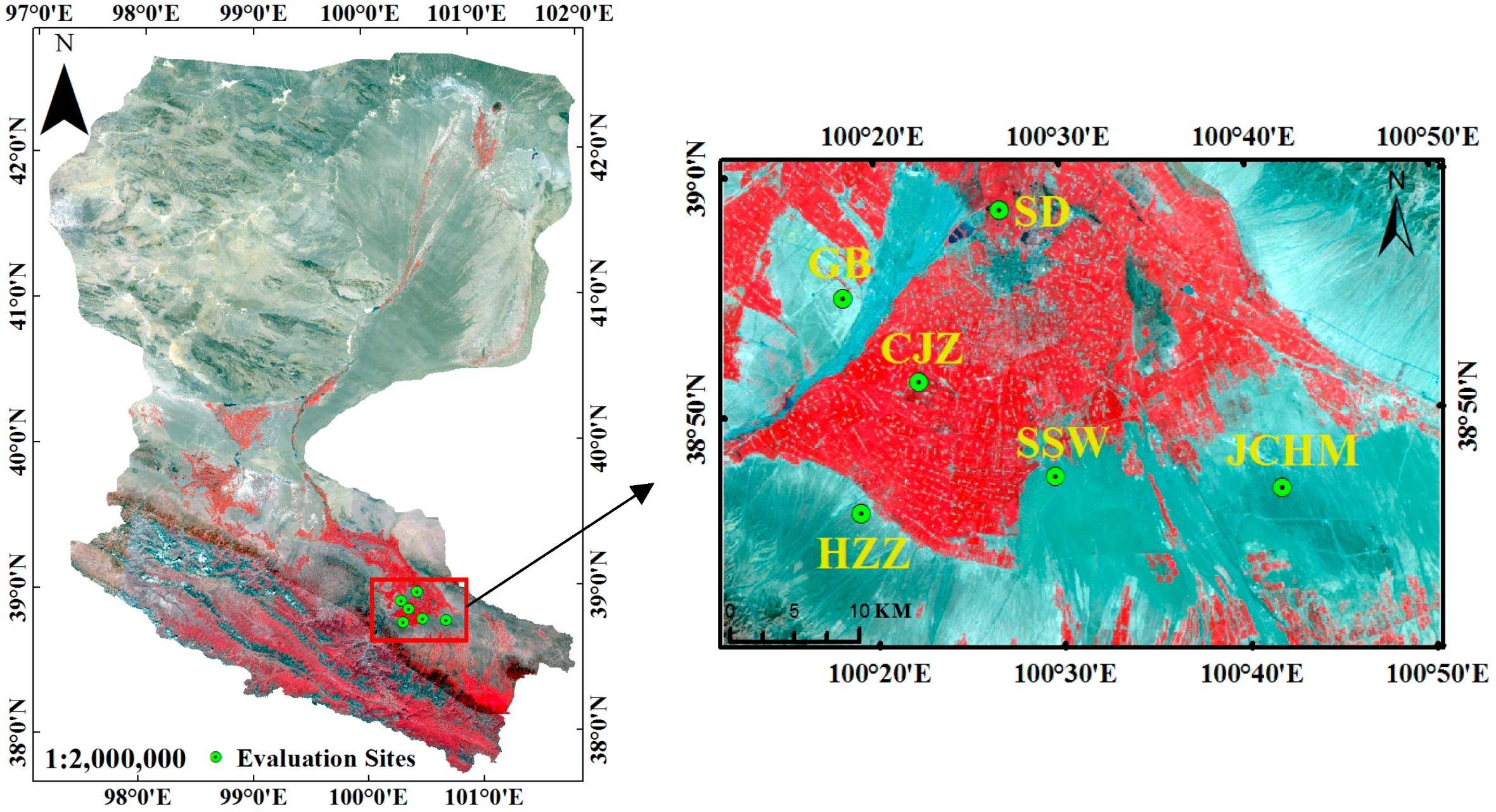
Figure 2.
Plot of the atmospheric transmittance (a) or upward radiance (b) at a given VZA against the atmospheric transmittance or upward radiance at nadir view.
Figure 2.
Plot of the atmospheric transmittance (a) or upward radiance (b) at a given VZA against the atmospheric transmittance or upward radiance at nadir view.
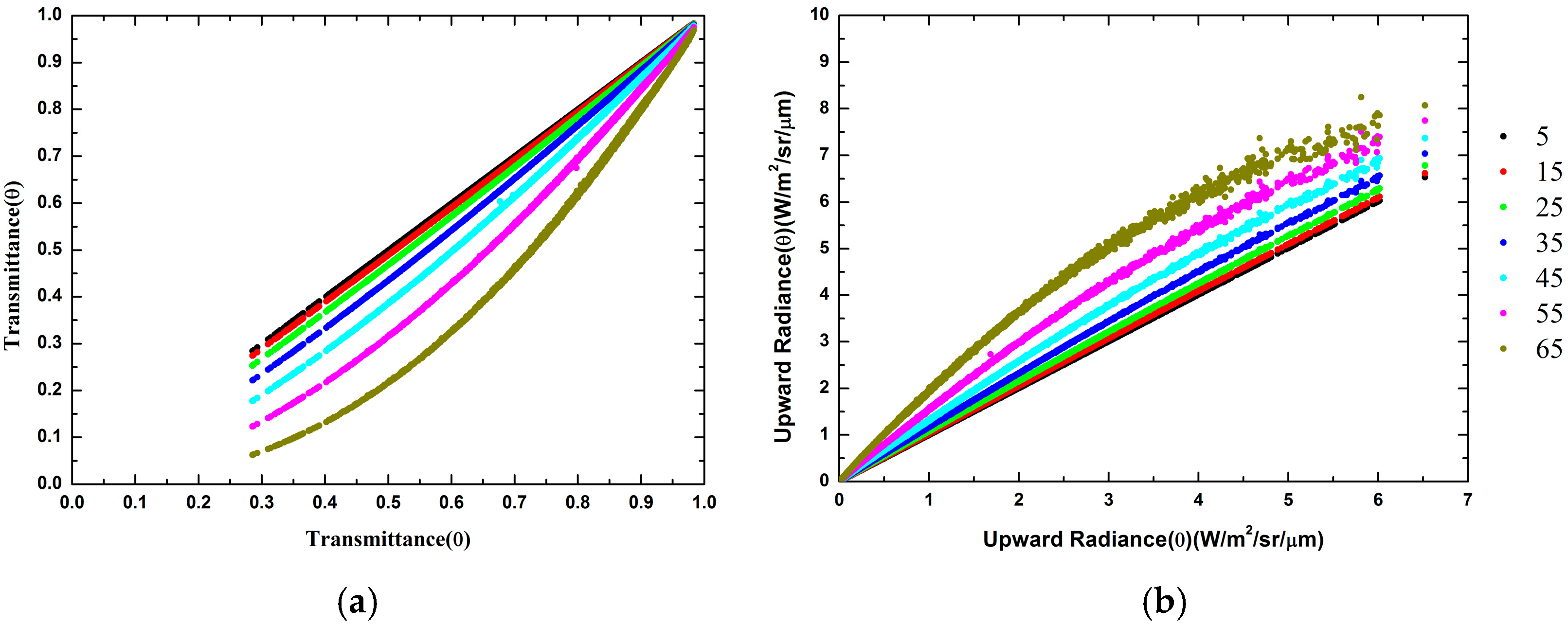
Figure 3.
Spectral response for band 5 of FY-3C/MERSI.

Figure 4.
Photos of measurement sites. (a) CJZ01; (b) CJZ02; (c) GB01; (d) SSW01; (e) SSW02,03; (f) GB02.
Figure 4.
Photos of measurement sites. (a) CJZ01; (b) CJZ02; (c) GB01; (d) SSW01; (e) SSW02,03; (f) GB02.

Figure 5.
LSE simulated by 4SAIL model varying LAI at a fixed soil emissivity of 0.96 (left) or a fixed leaf emissivity of 0.96 (right).
Figure 5.
LSE simulated by 4SAIL model varying LAI at a fixed soil emissivity of 0.96 (left) or a fixed leaf emissivity of 0.96 (right).
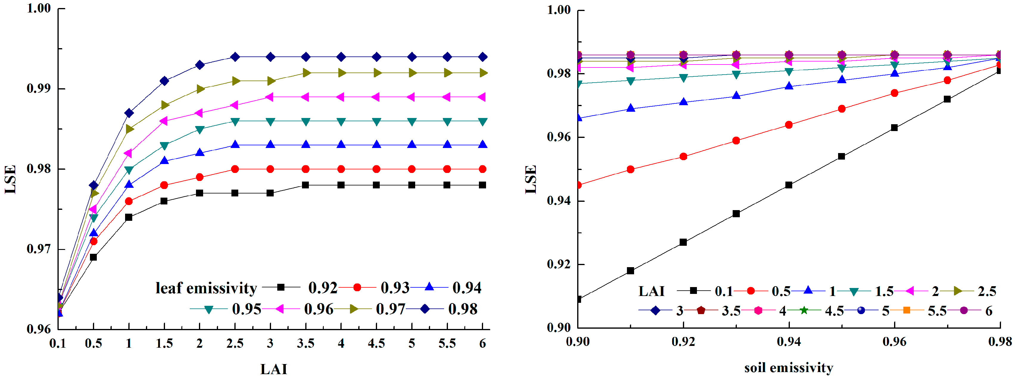
Figure 6.
The BBE of each eight-day period from 2001 to 2014 for six stations.
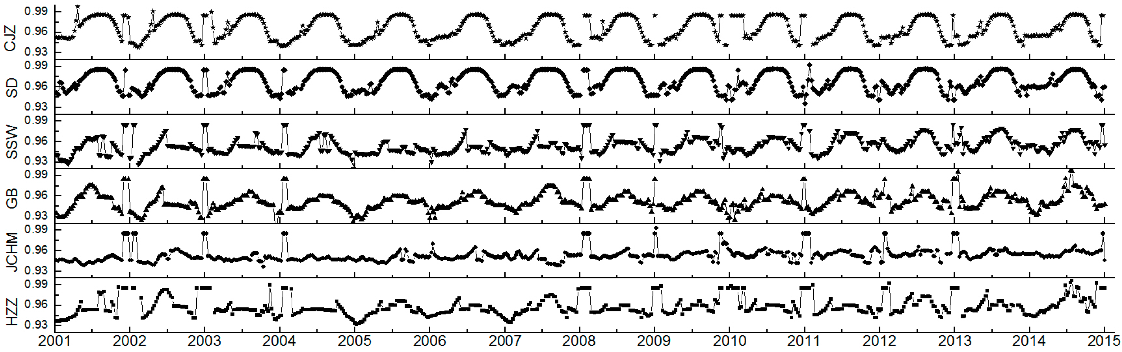
Figure 7.
Scatterplots between estimated LST from RTE algorithm (left) or GSC algorithm (right) and in situ LST.
Figure 7.
Scatterplots between estimated LST from RTE algorithm (left) or GSC algorithm (right) and in situ LST.
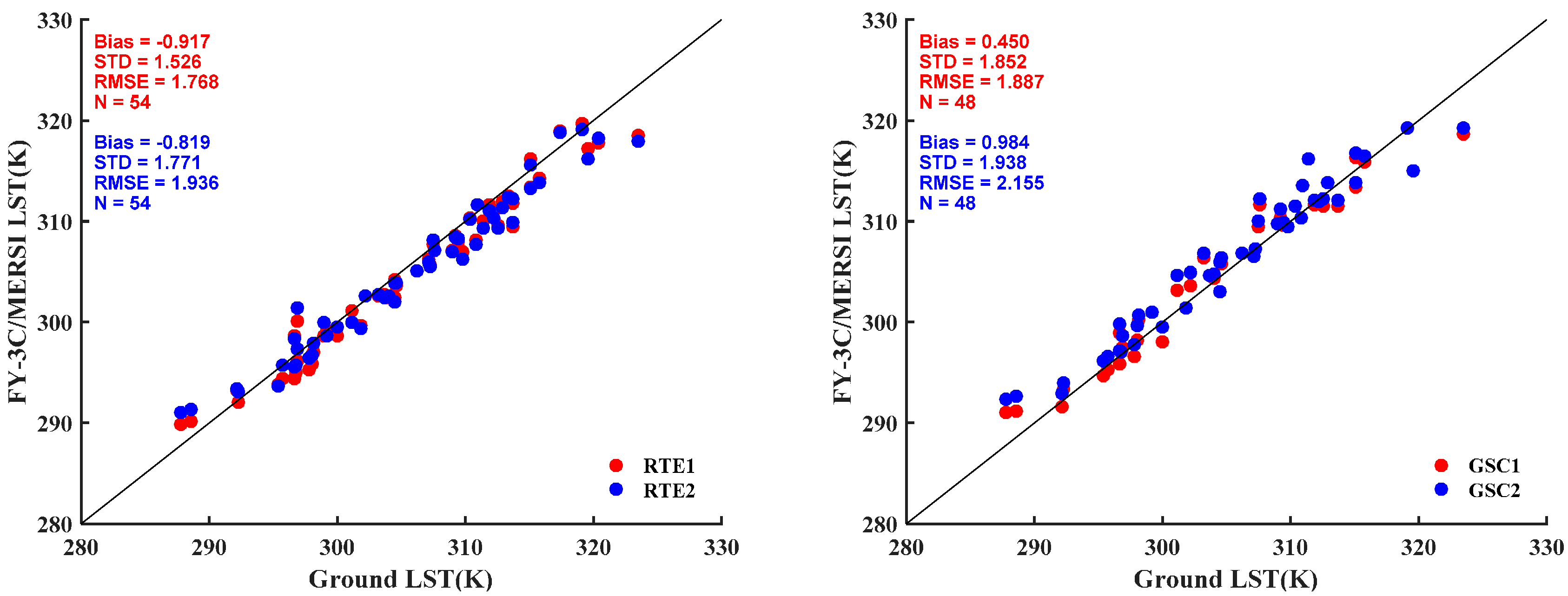
Figure 8.
The images and histograms of LSE difference between the AST_05 product and the new method on 17 and 26 July 2014; the corresponding images and histograms of LST difference. (a) The image of LSE difference on 17 July 2014; (b) The image of LSE difference on 26 July 2014; (c) The histogram of LSE difference on 17 July 2014; (d) The histogram of LSE difference on 26 July 2014; (e) The image of LST difference on 17 July 2014; (f) The image of LST difference on 26 July 2014; (g) The histogram of LST difference on 17 July 2014; (h) The histogram of LST difference on 26 July 2014.

Figure 9.
Boxplots between estimated LSTs from RTE algorithm (left) or GSC algorithm (right) at 250 m resolution and in situ LSTs.
Figure 9.
Boxplots between estimated LSTs from RTE algorithm (left) or GSC algorithm (right) at 250 m resolution and in situ LSTs.


Table 1.
Leaf emissivity values for five composited vegetation land cover types.
| IGBP Class | Composite Type | Leaf Emissivity | Sources |
|---|---|---|---|
| 1~7 | Forest and Shrubland | 0.967 | Mean of conifer and deciduous emissivity from ASTER spectral library and 24 leaf emissivities from MODIS spectral library and 10 measured leaf emissivities from Wang et al. [43] |
| 8, 9 | Savanna | 0.966 | 50% forest + 50% grassland |
| 10 | Grassland | 0.965 | Mean of green grass emissivity from ASTER spectral library and elephant grass emissivity from Pandya et al. [61] |
| 12, 14 | Cropland | 0.966 | Mean of 9 leaf emissivities from Pandya et al. [61], 4 wheat emissivities of Li et al. [36] and 39 measured leaf emissivities from Wang et al. [43] |
| 16, 254 | Other types | 0.966 | Mean value of above four types |
Table 2.
Angular Dependent Atmospheric correction coefficients of Equation (12) for FY3C/MERSI.
| Parameters | a1 | a2 | a3 | b1 | b2 | b3 | c1 | c2 | c3 |
|---|---|---|---|---|---|---|---|---|---|
| −0.0111 | −0.0846 | 0.0007 | −0.0955 | 0.9205 | 0.9997 | 0.0189 | −0.0198 | 0.0003 | |
| 0.1077 | 0.721 | −0.0055 | −0.2987 | −0.4775 | 1.0104 | 0.1885 | −0.2376 | −0.005 |
Table 3.
List of measured emissivities, estimated LSEs and the bias between them for different types.
Table 3.
List of measured emissivities, estimated LSEs and the bias between them for different types.
| Station Name | Type Name | Measured Emissivity | Estimated LSE Using the Method in Section 3.3 | Bias |
|---|---|---|---|---|
| CJZ01 | Corn leaf | 0.973 | 0.985 | 0.012 |
| CJZ02 | Chinese cabbage leaf | 0.987 | 0.985 | −0.002 |
| GB01 | Alhagi sparsifolia | 0.976 | 0.960 | −0.016 |
| SSW01 | Sparse vegetation | 0.986 | 0.971 | −0.015 |
| SSW02 | Large cluster sparse vegetation | 0.960 | 0.985 | 0.025 |
| SSW03 | Large cluster sparse vegetation | 0.959 | 0.962 | 0.003 |
| GB02 | Bare soil | 0.957 | 0.960 | 0.003 |
Table 4.
LSE estimated from AST_05 or the new method on 17 and 26 July 2014, as well as the corresponding LST.
Table 4.
LSE estimated from AST_05 or the new method on 17 and 26 July 2014, as well as the corresponding LST.
| 17 July 2014 | 26 July 2014 | |||||||
|---|---|---|---|---|---|---|---|---|
| Sites | LSEaster | LSEmersi | LSTaster (K) | LSTmersi (K) | LSEaster | LSEmersi | LSTaster (K) | LSTmersi (K) |
| SD | 0.955 | 0.984 | 300.566 | 298.887 | 0.955 | 0.984 | 302.115 | 300.447 |
| CJZ | 0.963 | 0.985 | 302.865 | 301.524 | 0.963 | 0.985 | 300.360 | 299.062 |
| GB | 0.954 | 0.955 | 312.475 | 312.401 | 0.954 | 0.957 | 315.341 | 315.154 |
| SSW | 0.954 | 0.964 | 317.890 | 317.179 | 0.954 | 0.967 | 318.487 | 317.616 |
| HZZ | 0.971 | 0.968 | 314.886 | 315.099 | 0.971 | 0.968 | 314.020 | 314.224 |
Table 5.
The average STD of the 3 × 3, 5 × 5, 7 × 7, 9 × 9, and 11 × 11 pixels extracted from 20 scenes of ASTER LST or ASTER LSE products at six stations.
Table 5.
The average STD of the 3 × 3, 5 × 5, 7 × 7, 9 × 9, and 11 × 11 pixels extracted from 20 scenes of ASTER LST or ASTER LSE products at six stations.
| LST STD (K) | LSE STD | |||||||||
|---|---|---|---|---|---|---|---|---|---|---|
| Sites | 3 × 3 | 5 × 5 | 7 × 7 | 9 × 9 | 11 × 11 | 3 × 3 | 5 × 5 | 7 × 7 | 9 × 9 | 11 × 11 |
| SD | 0.929 | 1.086 | 1.242 | 1.470 | 1.664 | 0.006 | 0.006 | 0.006 | 0.006 | 0.006 |
| CJZ | 0.804 | 1.041 | 1.387 | 1.801 | 1.977 | 0.005 | 0.005 | 0.005 | 0.005 | 0.005 |
| GB | 0.435 | 0.625 | 0.776 | 0.842 | 0.887 | 0.003 | 0.004 | 0.004 | 0.005 | 0.005 |
| SSW | 0.671 | 0.829 | 0.942 | 1.121 | 1.485 | 0.004 | 0.004 | 0.005 | 0.005 | 0.005 |
| HZZ | 0.396 | 0.468 | 0.530 | 0.601 | 0.684 | 0.003 | 0.004 | 0.004 | 0.004 | 0.005 |
| JCHM | 0.342 | 0.426 | 0.491 | 0.506 | 0.523 | 0.003 | 0.004 | 0.004 | 0.004 | 0.004 |
© 2017 by the authors. Licensee MDPI, Basel, Switzerland. This article is an open access article distributed under the terms and conditions of the Creative Commons Attribution (CC BY) license (http://creativecommons.org/licenses/by/4.0/).
Share and Cite
MDPI and ACS Style
Meng, X.; Cheng, J.; Liang, S. Estimating Land Surface Temperature from Feng Yun-3C/MERSI Data Using a New Land Surface Emissivity Scheme. Remote Sens. 2017, 9, 1247. https://doi.org/10.3390/rs9121247
AMA Style
Meng X, Cheng J, Liang S. Estimating Land Surface Temperature from Feng Yun-3C/MERSI Data Using a New Land Surface Emissivity Scheme. Remote Sensing. 2017; 9(12):1247. https://doi.org/10.3390/rs9121247
Chicago/Turabian StyleMeng, Xiangchen, Jie Cheng, and Shunlin Liang. 2017. "Estimating Land Surface Temperature from Feng Yun-3C/MERSI Data Using a New Land Surface Emissivity Scheme" Remote Sensing 9, no. 12: 1247. https://doi.org/10.3390/rs9121247
Note that from the first issue of 2016, this journal uses article numbers instead of page numbers. See further details here.