Comparison and Evaluation of the TES and ANEM Algorithms for Land Surface Temperature and Emissivity Separation over the Area of Valencia, Spain

Abstract

Land Surface temperature (LST) is a key magnitude for numerous studies, especially for climatology and assessment of energy fluxes between surface and atmosphere. Retrieval of accurate LST requires a good characterization of surface emissivity. Both quantities are coupled in a single radiance measurement; for this reason, for N spectral bands available in a remote sensor, there will always be N + 1 unknowns. To solve the indeterminacy, temperature-emissivity separation methods have been proposed, among which the Temperature Emissivity Separation (TES) algorithm is one of the most widely used. The Adjusted Normalized Emissivity Method (ANEM) was proposed as a modification of the Normalized Emissivity Method (NEM) algorithm by adjusting the initial emissivity guess using an estimation provided by the Vegetation Cover Method (VCM). In this work, both methods were applied to a set of five ASTER scenes over the area of Valencia, Spain, which were recalibrated and atmospherically corrected using local radiosoundings and ground measurements. These scenes were compared to the ASTER temperature and emissivity standard products (AST08 and AST05, respectively). The comparison to reference measurements showed a better agreement of ANEM LST in low spectral contrast surfaces, with biases of +0.4 K, +0.8 K for TES and +1.4 K for the AST08 product in a rice crop site. For sea surface temperature, bias was −0.1 K for ANEM, +0.3 K for TES and +1.3 K for the AST08 product. The larger differences of the AST08 product could be ascribed mainly to the atmospheric correction based on NCEP profiles in contrast to the local correction used in TES and ANEM and to a lesser extent the Maximum-Minimum Difference (MMD) empirical relationship used by TES. In terms of emissivity, ANEM obtained biases up to ±0.007 (positive over vegetation and negative over water), while TES biases were up to −0.015. The AST05 product showed differences up to −0.050, although for high contrast areas, such as sand surfaces, it showed better accuracy than both TES and ANEM. A comparison between TES and ANEM on four different classes within the scene showed a systematic difference between both algorithms, which was more pronounced for low spectral contrast surfaces. Therefore, ANEM improves the accuracy at low spectral contrast surfaces, while obtaining similar results to TES at higher spectral contrast surfaces, such as urban areas. The combination of both methods could provide a procedure benefiting from the strengths shown by each of them.

1. Introduction

Land Surface Temperature (LST) is one of the most important magnitudes for numerous climatological and meteorological processes, as the energy fluxes between surface and atmosphere for instance [1,2,3]. Retrieving accurate LSTs from remote sensing measurements depends on two essential issues: firstly, to make a correct characterization of the atmosphere, in order to remove the atmospheric effects on the at-sensor measurements; secondly, the Land Surface Emissivity (LSE) must be well known, with appropriate values for the analyzed bands [4]. However, LSE is commonly an unknown magnitude. For this reason, obtaining accurate LST and LSE values is a challenging goal in Thermal Infrared (TIR) remote sensing.

The main problem lays in the fact that for N TIR spectral bands, there exist N + 1 unknowns, corresponding to the respective emissivity channels and the LST value. Different temperature-emissivity separation algorithms, based on quasi-empirical models, have been proposed to solve this indetermination in the last two decades, e.g., [5,6,7,8,9,10,11]. Generally, these models assume an initial emissivity to make a first approach, which later is adjusted or improved.

One of the most used methods is the Temperature and Emissivity Separation (TES) algorithm, which has been studied in depth by different authors for different multispectral sensors [12,13,14,15,16]. This method starts from an initial emissivity guess for all pixels and channels (Normalized Emissivity Method or NEM module) and uses an empirical relationship (Maximum-Minimum Difference, or MMD module) that allows estimating the minimum emissivity of the spectrum by taking into account the spectral contrast, thus to obtain the emissivity for all channels.

Coll et al. proposed in [17,18] the Adjusted Normalized Emissivity Method (ANEM) based on the NEM [19], which is estimated using the vegetation cover method proposed in [20], which relates for each pixel the effective emissivity to the fractional vegetation cover calculated previously from a vegetation index.

Presently, most remote sensing missions tend to integrate hyperspectral sensors, with several spectral bands in the thermal infrared region. In this manner, these empirical models will contribute to the LST and LSE retrieval from thermal infrared measurements in near future hyperspectral missions, like the HyspIRI mission. In this context, the comparison of the TES and ANEM algorithms, which has not been performed before, can be of interest.

ASTER, launched on 19 December 1999 aboard the Terra satellite, is a multispectral sensor provided with 15 spectral bands (4 Visible and Near-Infrared Bands (VNIR), 6 Shortwave Infrared Bands (SWIR) and 5 Thermal Infrared Bands (TIR)). ASTER offers high resolution imagery for the TIR region (90 m), with LST and emissivity products (AST08 and AST05, respectively) based on the TES method. Validation studies [16,21,22,23] have shown the agreement of these products within the predicted uncertainty values of ±1.5 K for temperature and ±0.015 for emissivity. Despite this, some authors suggest improvements to the product algorithm in order to reduce that uncertainty, most of them related to atmospheric correction [13,24,25].

In this paper, ASTER products AST05 and AST08 were compared with TES and ANEM algorithms applied to ASTER L1 scenes, which were previously calibrated and corrected atmospherically using local radiosoundings and ground measurements. The aim of this work is to evaluate the ANEM algorithm in comparison to the TES algorithm in ASTER scenes over different surface types. To reach the objective, five ASTER L1 scenes and ASTER LST and LSE and emissivity products over the Valencia area, Spain, were used, covering different surface types such as rice crops and other agricultural sites, water and urban areas.

The paper proceeds as follows. Section 2 presents the study area and data. Then, in Section 3, the methodology applied to carry out the study, corresponding to TES and ANEM methods, is presented. Section 4 shows the results obtained, while the corresponding discussion is presented in Section 5. Finally, the main conclusions of the work are given in Section 6.

2. Study Area & Data

2.1. Study Area

This study was carried out over the Mediterranean coast near the city of Valencia, Spain (see Figure 1). This area covers different surface types including Valencia city, many smaller urban centers and industrial areas (seen in gray in Figure 1), the Albufera Lake with rice crops around it, agricultural areas corresponding to other crops (mainly orange groves, seen in orange-red in Figure 1), Mediterranean forest areas (seen in brown in Figure 1) and the Mediterranean Sea.

The study area is characterized by the Mediterranean climate. It is a typically hot climate during the summer season. Maximum temperatures are close to 308 K; the minimum ones are around 293 K; and rain is scarce in this period of the year. The orography of the area is varied, with altitudes from sea level to 800 m, although most part of the zone is below 300 m.

2.2. Data

Five ASTER L1B scenes that provided the Top of Atmosphere (TOA) radiances required to apply the analyzed methods were used. These scenes were selected from all ASTER L1B scenes available for the study area taking into account two main reasons, which make the evaluation conditions optimum: the homogeneity of the surface existing during the summer period at the rice crops and the availability of in situ radiosounding profiles launched concurrently with the ASTER overpasses. They were recorded on 3 August 2004, 12 August 2004, 21 July 2005, 24 July 2006 and 11 July 2007. The atmospheric correction was applied to the different scenes and channels in order to obtain the corresponding at-surface radiances required by the methods. The results were compared with ground data measured over the rice fields concurrent to the satellite overpass, with the Sea Surface Temperature (SST) product from the MODIS sensor and also with the ASTER emissivity and temperature standard products (AST05 and AST08, respectively).

2.2.1. ASTER Sensor

ASTER provides high resolution images of the Earth at 14 different bands of the electromagnetic spectrum, with two Visible and two Near-Infrared (VNIR) bands, six Shortwave Infrared (SWIR) bands and five Thermal Infrared (TIR) bands. The viewing angle is close to nadir (<8.5°). The spatial resolution depends on the sensor spectral band, with 15 m for VNIR, 30 m for SWIR and 90 m for the TIR (see

Table 1. Wavelength and spatial resolution of each ASTER band.

Spectral Range	ASTER Band	Wavelength (µm)	Spatial Resolution (m)
VNIR	1	0.520–0.600	15
	2	0.630–0.690
	3n	0.760–0.860
	3b	0.760–0.860
SWIR	4	1.600–1.700	30
	5	2.145–2.185
	6	2.185–2.225
	7	2.235–2.285
	8	2.295–2.365
	9	2.360–2.430
TIR	10	8.125–8.475	90
	11	8.475–8.825
	12	8.925–9.275
	13	10.250–10.950
	14	10.950–11.650

).

The VNIR data (ASTER Bands 2 and 3n) were used to calculate the NDVI needed to retrieve the ANEM emissivity as shown in the next section. The digital numbers were transformed to at-sensor radiances according to:

$$L_{TOA,i}=\left(D{N}_i-1\right)UC{C}_i$$

(1)

where $UC{C}_i$ are the unit conversion coefficients given in the scene metadata, which take values of 0.708 and 0.862 W m⁻² sr⁻¹ µm⁻¹ for Bands 2 and 3, respectively. Then, L_TOA,i was converted to at-surface reflectance using the image-based atmospheric correction model of Chavez et al. proposed in [26], based on Dark-Object Subtraction (DOS model). This model corrects the at-sensor radiance subtracting the path radiance, before calculating the at-surface reflectance.

For the TIR bands, at-surface radiances are needed to apply the TES and ANEM methods. To increase the precision and accuracy of the at-surface radiances, the local calibration and atmospheric correction proposed in [21] were applied instead of the ASTER standard calibration. This combined local calibration and atmospheric correction was given by a linear function of DN_i:

$$L_{surf,i}=a_{i}D{N}_i+b_i$$

(2)

where coefficients $a_i$ and $b_i$ depend on the band and date of the scene, $L_{surf,i}$ being the at-surface recalibrated and atmospherically-corrected radiances at band $i$. These coefficients were retrieved using simulated radiances from the radiative transfer code MODTRAN 4 [27] with atmospheric profiles of pressure, temperature and moisture measured using an RS80 radiosonde balloon launched at the study area at the time of satellite overpass (details are given in [21]). The use of ground measurements reduces the $L_{surf,i}$ uncertainties due to calibration and atmospheric correction, so the application of the ANEM and TES methods should provide, in principle, more accurate results than the standard ASTER products. Coefficients used in Equation (2) for all dates are presented in

Table 2. Coefficients a_i (W m⁻² sr⁻¹ µm⁻¹/DN) and b_i (W m⁻² sr⁻¹ µm⁻¹) to apply the combined local calibration and atmospheric correction for the scenes used in the present study (given in [21]) for 2004 and 2005 and derived here for 2006 and 2007. The correlation coefficients of each linear function are also provided.

Date	Band	ai	bi	r2
3 August 2004	10	0.012908	−5.982	0.9996
	11	0.010369	−3.682	0.9998
	12	0.009087	−2.687	0.9997
	13	0.007389	−2.451	1.0000
	14	0.007210	−3.057	0.9989
12 August 2004	10	0.012796	−6.113	0.9994
	11	0.010419	−3.859	0.9997
	12	0.008995	−2.640	0.9994
	13	0.007430	−2.587	1.0000
	14	0.007320	−3.378	1.0000
21 July 2005	10	0.013155	−6.639	0.9993
	11	0.010774	−4.480	1.0000
	12	0.009265	−3.131	0.9996
	13	0.007538	−2.831	1.0000
	14	0.007602	−3.908	0.9986
24 July 2006	10	0.013970	−7.445	0.9995
	11	0.011175	−4.933	0.9986
	12	0.009451	−3.379	0.9998
	13	0.007779	−3.221	1.0000
	14	0.007852	−4.313	0.9996
11 July 2007	10	0.014565	−7.297	0.9956
	11	0.011427	−4.663	0.9991
	12	0.009836	−3.523	0.9989
	13	0.008485	−3.940	1.0000
	14	0.008629	−5.136	0.9993

for each band.

ASTER L2 standard products of emissivity and temperature (AST05 and AST08, respectively) were used as a reference to compare with the images obtained with the analyzed methods. AST05 and AST08 products are obtained by the TES algorithm, with a spatial resolution of 90 m. The nominal accuracy of these products are ±1.5 K for AST 08 and ±0.015 for AST05 [28]. These products use the radiative transfer model MODTRAN 3.5 with required atmospheric parameters obtained from the National Center of Environmental Prediction and the National Center of Atmosphere Research (NCEP and NCAR) and satellite data [23,29].

2.2.2. Reference Measurements

In order to evaluate the results obtained with the different methodologies, temperature and emissivity values for different surface types measured by Coll et al. [21] and Niclòs et al. [30] in the field were used.

One of the major difficulties with the evaluation of remote sensing data is the difference between the spatial scales of satellite and ground measurements. In this case, that ASTER sensor has a spatial resolution of 90 m in the TIR, but the spatial scale of ground radiometric measurements is usually lower than 1 m. In order to make the two types of measurements compatible, it is necessary to consider wide and homogeneous reference areas, both in temperature and emissivity. Consequently, water (Mediterranean Sea) and vegetation with complete cover (rice fields around Albufera Lake) were used for the evaluation and comparison.

The temperature of rice-covered surfaces was obtained through in situ radiometric measurements concurrent to the ASTER overpass, between 10:54 and 11:00 UTC depending on the data. Two CIMEL 312 radiometers [31] were used, for which the temperature measurements corresponding to 3 min around the satellite overpass were considered for evaluation. The mean value and standard deviation of those temperatures were calculated, the latter giving an estimate of the natural variability of ground temperatures in the area. The average radiometric temperature was corrected for emissivity and atmospheric effects using measurements of emissivity and atmospheric downwelling irradiance. The uncertainty associated with the in situ-measured LST includes the radiometer calibration uncertainties, the emissivity correction uncertainties and the natural variation of the surface temperature (see [21] for details). The retrieved LSTs and uncertainties for the rice field evaluation site are shown in

Table 3. Ground LST values and uncertainties measured in situ at the rice field concurrent to the ASTER overpass. MODIS-Terra SST product values (mean and standard deviation for 3 × 3 pixels centered at the location shown as latitude/longitude) from the Mediterranean Sea and the total precipitable water (TPW) are also given.

Date	TPW (cm)	Rice Field			Mediterranean Sea
		LST (K)	δ (K)	Location	SST (K)	δ (K)	Location
3 August 2004	2.35	303.6	0.7	39.250°N, 0.295°W	299.3	0.4	39.250°N, 0.295°W
12 August 2004	2.05	302.0	0.5	39.250°N, 0.295°W	299.6	0.5	39.250°N, 0.295°W
21 July 2005	2.03	301.6	0.6	39.265°N, 0.308°W	299.8	0.4	39.250°N, 0.295°W
24 July 2006	2.39	302.4	0.9	39.265°N, 0.308°W	301.0	0.4	39.250°N, 0.295°W
11 July 2007	2.90	300.3	0.3	39.265°N, 0.308°W	297.9	0.4	39.250°N, 0.295°W

. Additionally,

Table 4. Rice and sand beach emissivity values with their standard deviations (Std) retrieved from ground measurements using Temperature Emissivity Separation (TES) with CIMEL 312-2 and Mediterranean Sea emissivity using CIMEL CE312-2 and Negative Temperature Coefficient (NTC) thermistors.

CE 312 Band	λi (µm)	Rice Field		Sand Beach		Mediterranean Sea
		ε	Std	ε	Std	ε	Std
6	8.42	0.970	0.012	0.820	0.011	0.980	0.006
5	8.68	0.980	0.015	0.813	0.009	0.984	0.005
4	9.15	0.978	0.015	0.796	0.010	0.984	0.004
3	10.57	0.982	0.010	0.951	0.005	0.990	0.004
2	11.30	0.982	0.008	0.956	0.003	0.991	0.004

shows the emissivity of the rice crops and also of the sand at the nearby beach that were measured in situ for the five bands of the CIMEL 312-2 radiometer through the TES method adapted to that radiometer [32].

To compare the ASTER-derived water temperature, the MODIS-Terra SST product MOD28 [33] with 1 km of spatial resolution was used. The SST was obtained for a window 3 × 3 of each MODIS scene and compared against a window of 33 × 33 pixels of ASTER centered on the same coordinates. Table 3 shows the MOD28 SST values together with their uncertainty, calculated as the quadratic sum of the SST standard deviation for the 3 × 3 pixels and the product uncertainty established by Niclòs et al. in [34]. This last uncertainty has a value of ±0.37 and was obtained as a result of a MOD28 product validation with in situ measurements. Water emissivity values, shown in Table 4, were measured in [30] for the six CE312-2 bands. A sample of Mediterranean Sea water was used to obtain the emissivity from measurements of the surface and sky radiance with two CE312-2 radiometers and the surface temperature with several Negative Temperature Coefficient (NTC) thermistors (see [30] for more details).

3. Methodology

3.1. TES Algorithm

The Temperature-Emissivity Separation (TES) method was first proposed in [10] to obtain LST and LSE from the five TIR ASTER channels. TES is applied to channel i at-surface radiance (L_surf,i), as given by Equation (3):

$$L_{surf,i}={\epsilon }_i{B}_i\left(T\right)+\frac{\left(1-{\epsilon }_i\right)F_{atm,i}}{\pi }$$

(3)

where $B_i\left(T\right)$ is Planck’s function for the effective wavelength λ_i of each ASTER band at surface temperature T, ${\epsilon }_i$ is the channel emissivity and $F_{atm,i}$ is the downwelling atmospheric irradiance. TES starts with the Normalized Emissivity Method (NEM) module [19], in which the at-surface radiances obtained from the atmospherically-corrected at-sensor radiances are introduced into Equation (3) using an initial surface emissivity value, generally 0.99, for all channels and pixels, and the Planck radiance $B_i\left(T\right)$ is retrieved for each band:

$$B_i\left(T\right)=\frac{\left[L_{surf,i}-\frac{\left(1-{\epsilon }_i\right)F_{atm,i}}{\pi }\right]}{{\epsilon }_i}$$

(4)

Planck radiances are then inverted obtaining five temperature values. The maximum temperature value (T_NEM) is chosen as the first approximation to the LST. Using T_NEM in Equation (3), new emissivity values are retrieved for each band (${\epsilon }_{NEM,i}$):

$${\epsilon }_{NEM,i}=\frac{\left(L_{surf,i}-\frac{F_{atm,i}}{\pi }\right)}{\left(B_i\left(T_{NEM}\right)-\frac{F_{atm,i}}{\pi }\right)}$$

(5)

${\epsilon }_{NEM,i}$ values are used to retrieve the temperature-independent ${\beta }_i$ index ($\beta$ spectrum):

$${\beta }_i=\frac{{\epsilon }_{NEM,i}}{\overline{\epsilon }}$$

(6)

where $\overline{\epsilon }$ is the mean value of NEM emissivities of the five TIR bands. Then, the difference between maximum and minimum β values is calculated (maximum-minimum difference or MMD). The MMD is related to the minimum value of the emissivity spectrum (${\epsilon }_{min}$) in accordance with an empirical relationship (calibration curve), which is obtained using a set of spectra of rocks, soils, vegetation, snow and water given in the ASTER library [35]. Hulley and Hook in [12] obtained a new expression, which adjusts better to vegetated covers since they used a larger number of vegetated cover types to estimate the MMD regression curve, which is:

$${\epsilon }_{min}=0.9951-0.7264\times MM{D}^{0.7873}$$

(7)

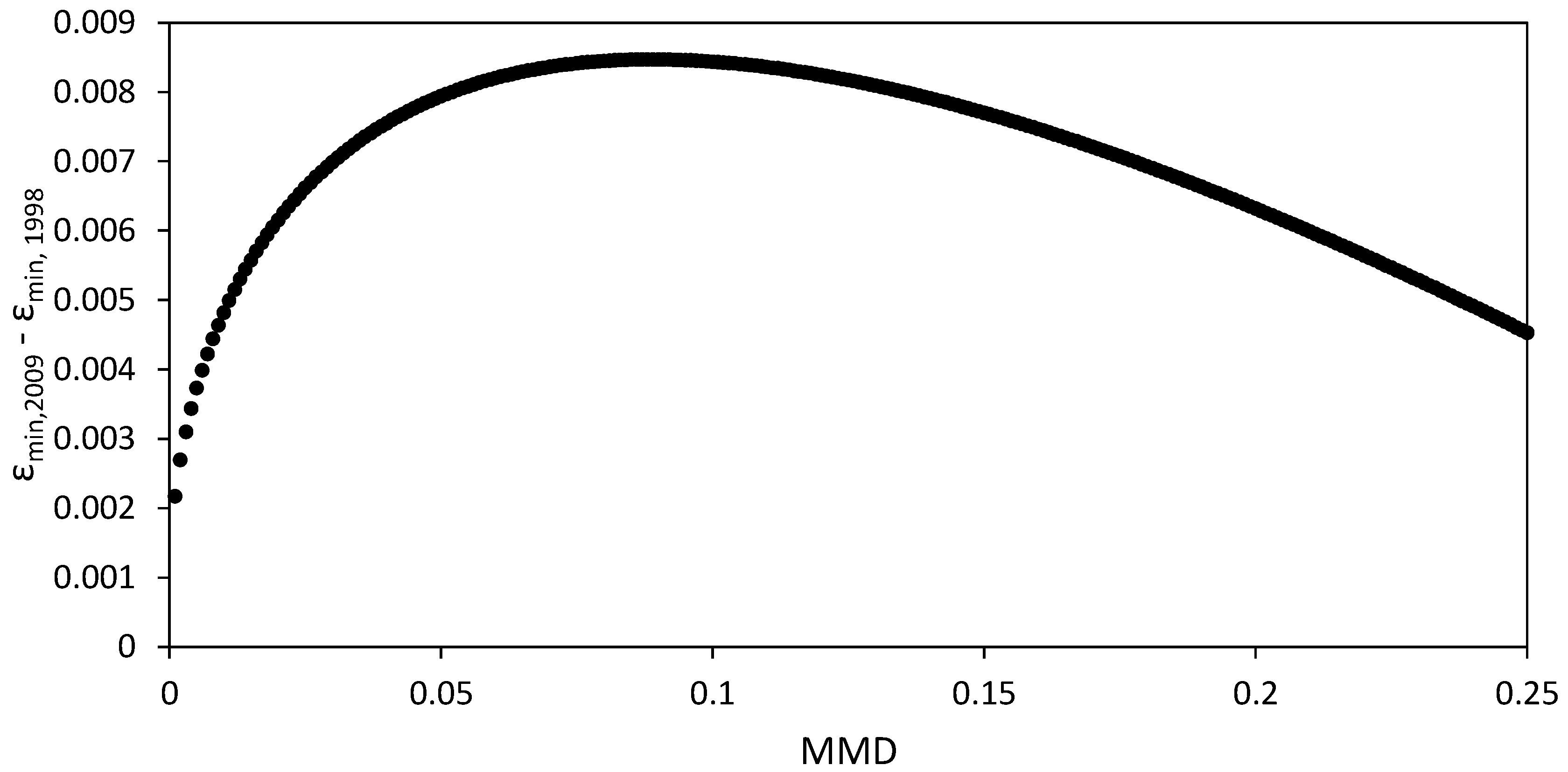
This expression was compared with the one given by Gillespie et al. in [10]. The difference between both expressions according to the MMD value is shown in Figure 2. This difference is higher for MMD values between 0.05 and 0.15, showing a maximum disagreement up to 1% in the minimum emissivity estimation.

Finally, the emissivity spectrum is calculated using ${\epsilon }_{min}$ together with the β spectrum.

$${\epsilon }_i={\epsilon }_{min}\frac{{\beta }_i}{min\left({\beta }_i\right)}$$

(8)

The emissivity spectra obtained from Equation (8) are then used in Equation (4), from which five new temperatures are retrieved. These new temperatures should be equal, but often, they present small differences. If these differences are lower than the noise equivalent temperature difference (NEΔT) of ASTER (±0.3 K), then the maximum of the obtained temperature values is considered as the best estimate of LST.

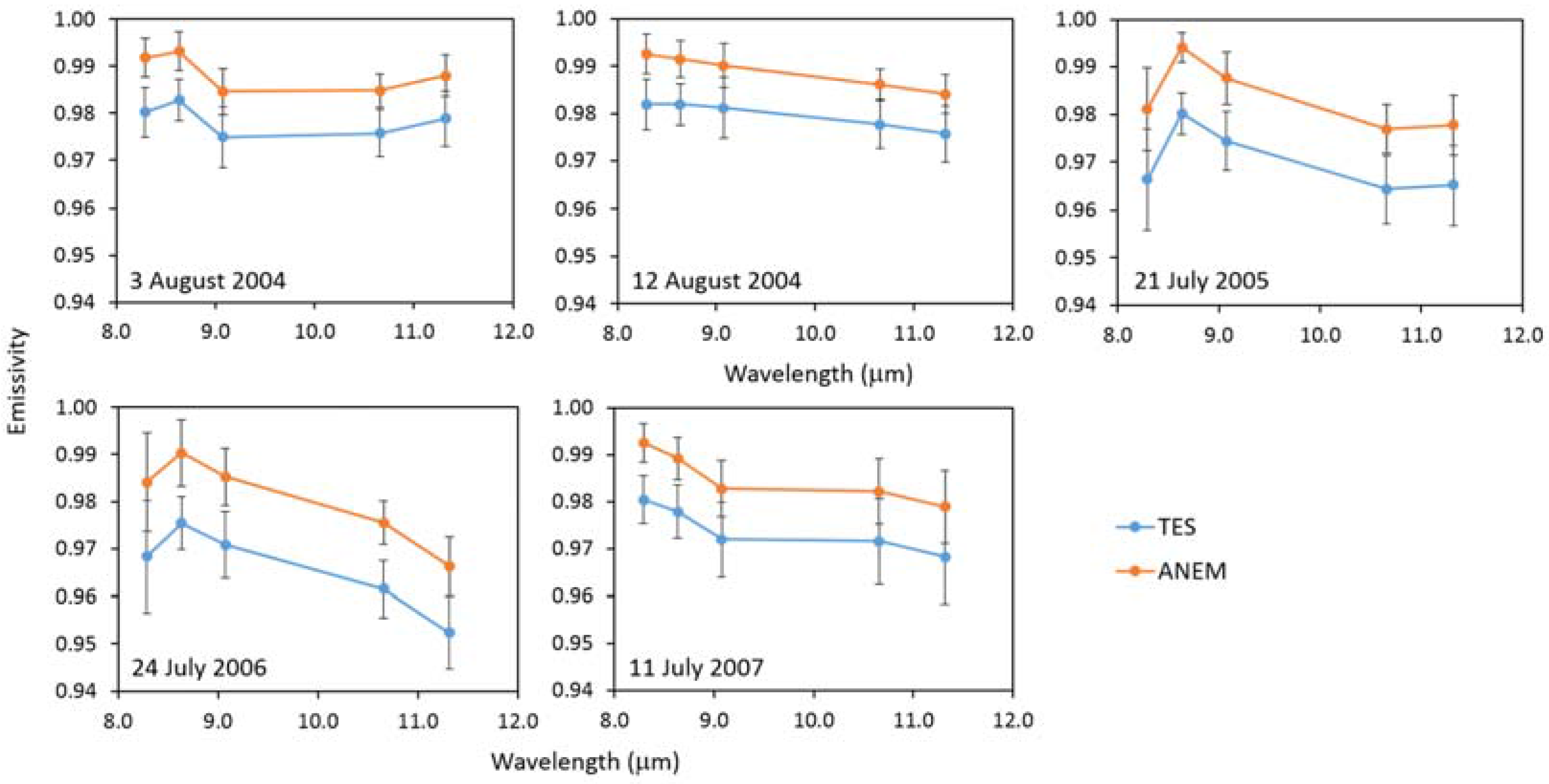
3.2. ANEM Algorithm

The Adjusted Normalized Emissivity Method (ANEM) was proposed in [18] as a combination of the Vegetation Cover Method (VCM) [20,36] and NEM [19], explained in Section 3.1. In ANEM, the emissivity introduced as the input in NEM is retrieved with VCM depending on the vegetation fraction of each pixel in the scene. As a consequence, a different value of emissivity is used for each pixel as initial emissivity for NEM, instead of a unique value for all pixels.

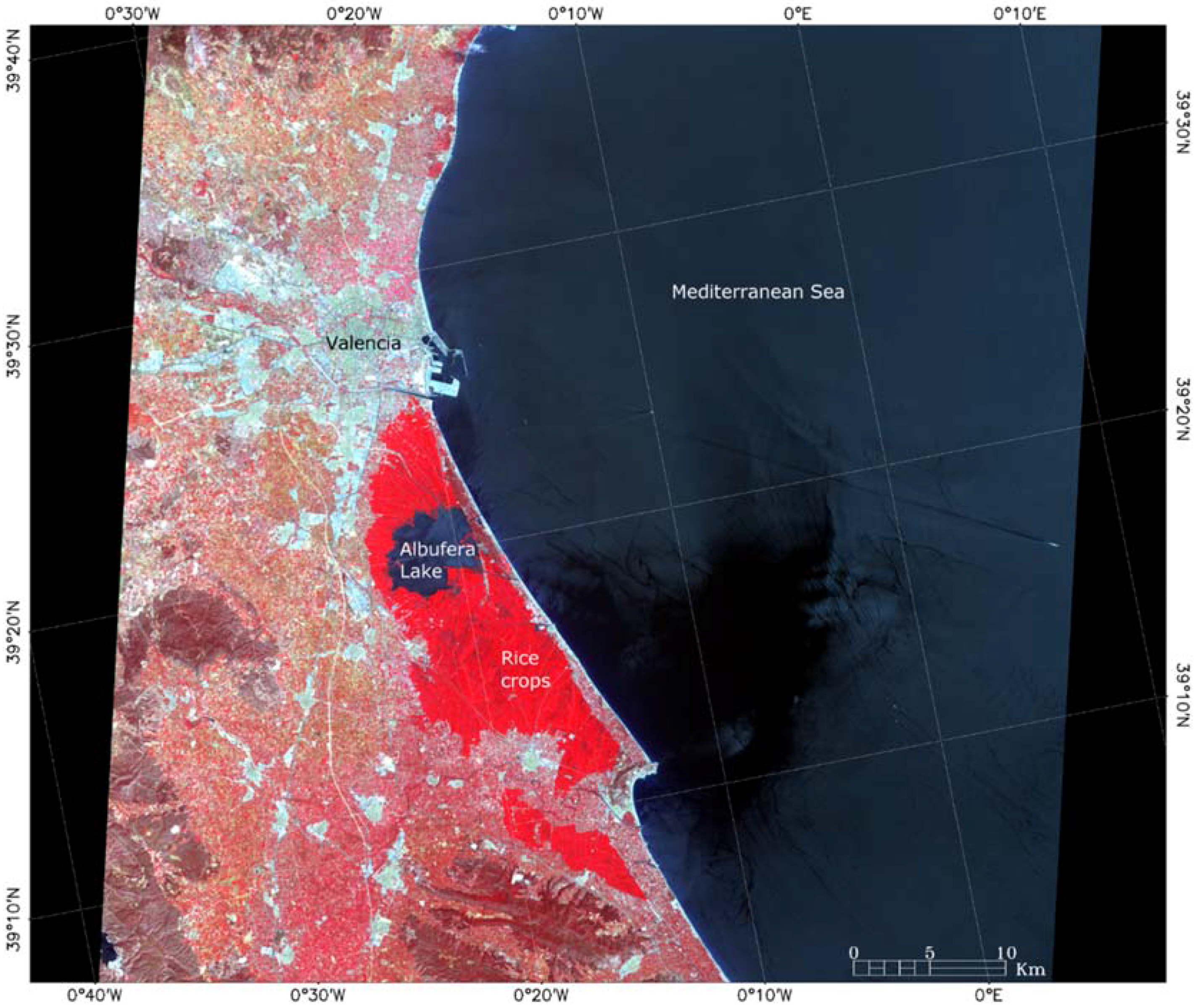
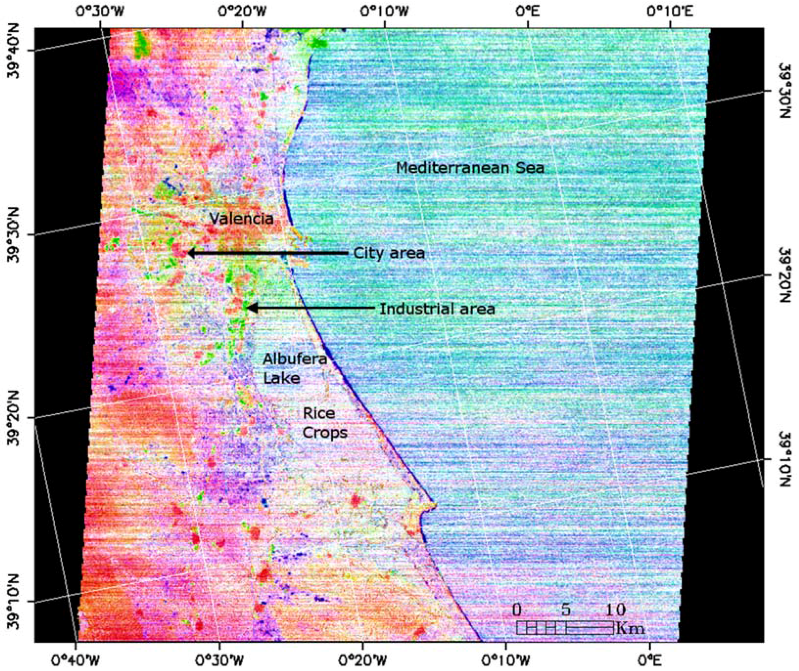
To apply ANEM, it is required to distinguish between natural areas, urban areas and water using the corresponding masks in the scene. They were obtained using ASTER Shortwave Infrared (SWIR) bands (Bands 4–9) with a supervised classification using a Mahalanobis distance of 30 m. We selected the following regions of interest: natural areas including different types of agricultural fields (mainly rice paddies and orange groves) and forested areas; urban areas such as the city of Valencia and other smaller towns around it; and water areas of the Mediterranean Sea and the Albufera Lake. The VCM is applied for natural areas. The effective emissivity of a heterogeneous and rough surface is calculated as:

$${\epsilon }_i={\epsilon }_{vi}{P}_v+{\epsilon }_{si}\left(1-P_v\right)+4\langle d{\epsilon }_i\rangle P_v\left(1-P_v\right)$$

(9)

where ${\epsilon }_{vi}$ and ${\epsilon }_{si}$ are the emissivities of vegetation and soil pixels in band i, respectively, $P_v$ is the vegetation fractional cover and $\langle d{\epsilon }_i\rangle$ is a term related to the internal reflections between vegetation and soil that depend on the surface structure (cavity term), which is given in [37]:

$$\langle d{\epsilon }_i\rangle =-0.435{\epsilon }_{si}+0.4343$$

(10)

The ${\epsilon }_{vi}$ and ${\epsilon }_{si}$ values (see

Table 5. Emissivity of vegetation (${\epsilon }_{vi}$), soil (${\epsilon }_{si}$) and cavity term ($\langle d{\epsilon }_i\rangle$) to be used in the Vegetation Cover Method (VCM) for the different ASTER TIR channels (see Equation (9)). The indicated uncertainties correspond to the standard deviation of the emissivity values for all the considered samples.

Band	${\mathit{\epsilon }}_{\mathit{v}\mathit{i}}$	${\mathit{\epsilon }}_{\mathit{s}\mathit{i}}$	$\mathbf{\langle }\mathit{d}{\mathit{\epsilon }}_{\mathit{i}}\mathbf{\rangle }$
10	0.990 ± 0.002	0.92 ± 0.05	0.03 ± 0.02
11	0.986 ± 0.005	0.93 ± 0.05	0.03 ± 0.02
12	0.979 ± 0.015	0.93 ± 0.04	0.031 ± 0.017
13	0.985 ± 0.005	0.970 ± 0.006	0.012 ±0.003
14	0.988 ± 0.003	0.971 ± 0.005	0.012 ± 0.002

) were estimated from the spectra provided in the ASTER spectral library. For vegetation, ${\epsilon }_{vi}$ was calculated as the average emissivity of green vegetation samples (grass and conifer) for each of the five ASTER TIR bands; while for soil, the procedure is the same, but using 65 soil samples, including 23 aridisols, 11 entisols, 10 mollisols, 9 alfisols, 8 inceptisols, 2 vertisols, 1 spodosol and 1 ultisol. Before the estimation, the different emissivity spectra were integrated with the filter functions of the five ASTER TIR channels to get band-integrated emissivities corresponding to each spectrum.

Different values of vegetation fraction between 0 and 1 were introduced into Equation (9) together with the coefficients given in Table 5. For each value of P_v, five different effective emissivity values were retrieved, one per band, then the maximum value was taken. The obtained emissivity maximum values were adjusted against P_v, with a correlation coefficient of 0.987, resulting in Equation (11), which directly provides the maximum emissivity value to be introduced into NEM as a function of the vegetation fraction:

$${\epsilon }_{max}=0.9938P_v+0.9699\left(1-P_v\right)+0.044P_v\left(1-P_v\right)$$

(11)

The vegetation fraction needed in Equation (11) was calculated following the procedure proposed in [20]:

$$P_v=\frac{\left(1-\frac{i}{i_s}\right)}{\left(1-\frac{i}{i_s}\right)-K\left(1-\frac{i}{i_v}\right)}$$

(12)

where $i$ is the Normalized Difference Vegetation Index (NDVI) [38] of each pixel,$i_s$ and $i_v$ are the minimum and maximum NDVI values of the area, which are representative of bare soil and dense vegetation, respectively, and $K=\left({\rho }_{3v}-{\rho }_{2v}\right)/\left({\rho }_{3s}-{\rho }_{2s}\right)$, where ${\rho }_{is}$ (${\rho }_{iv}$) is the at-surface reflectance value in the red (ASTER Band 2) and near-infrared (ASTER band 3) over pixels where the values $i_s$ ($i_v$) are found. Then, the NDVI image was resized to the SWIR pixel size in order to take the $i_s$ and $i_v$ values from the histogram of the scene taking into consideration only the pixels belonging to the natural areas mask. Using the cumulative histogram, the mean value of the pixels between percentiles 4 and 7 was used to calculate $i_s$, while the mean of the pixels with percentiles between 93 and 96 of the NDVI distribution was used to obtain $i_v$.

Since the previous procedure is not applicable in the case of urban zones and water surfaces, an input emissivity value for the NEM module was determined for them. For water, the emissivity values for the ASTER channels were obtained from Niclòs et al. in [30] (see Table 4). The maximum value was taken as ε_max = 0.991 corresponding to ASTER Band 14.

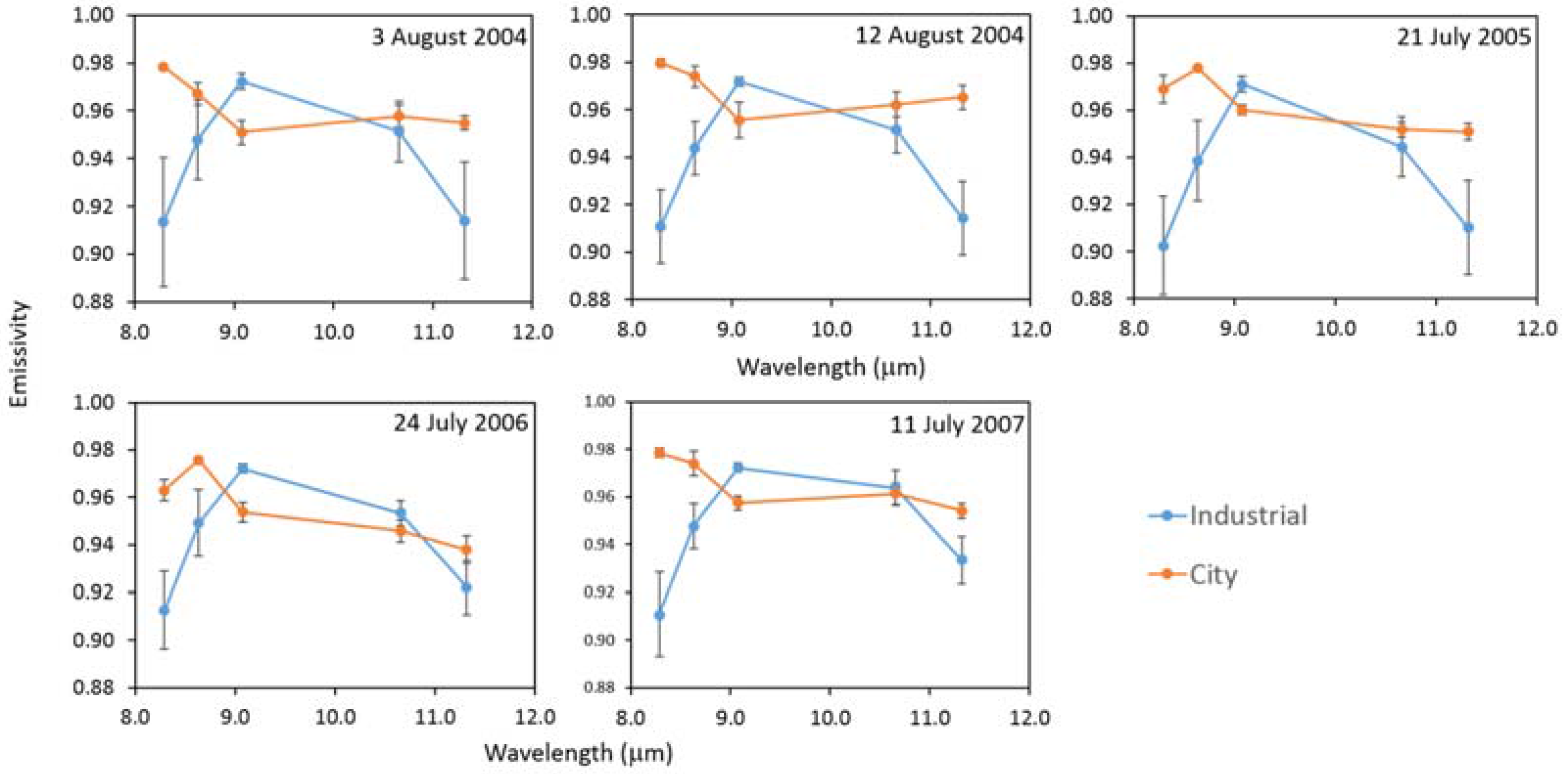
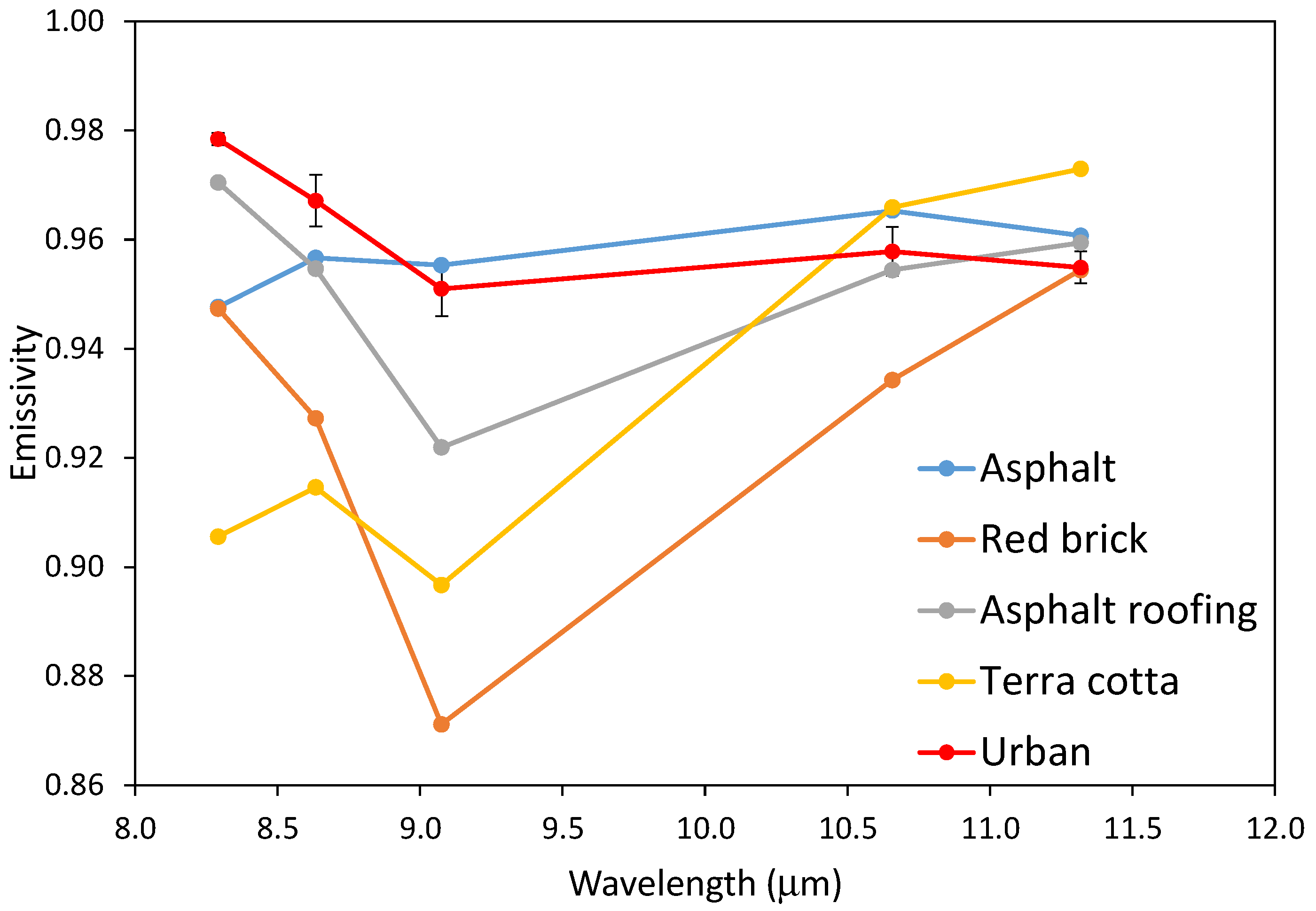
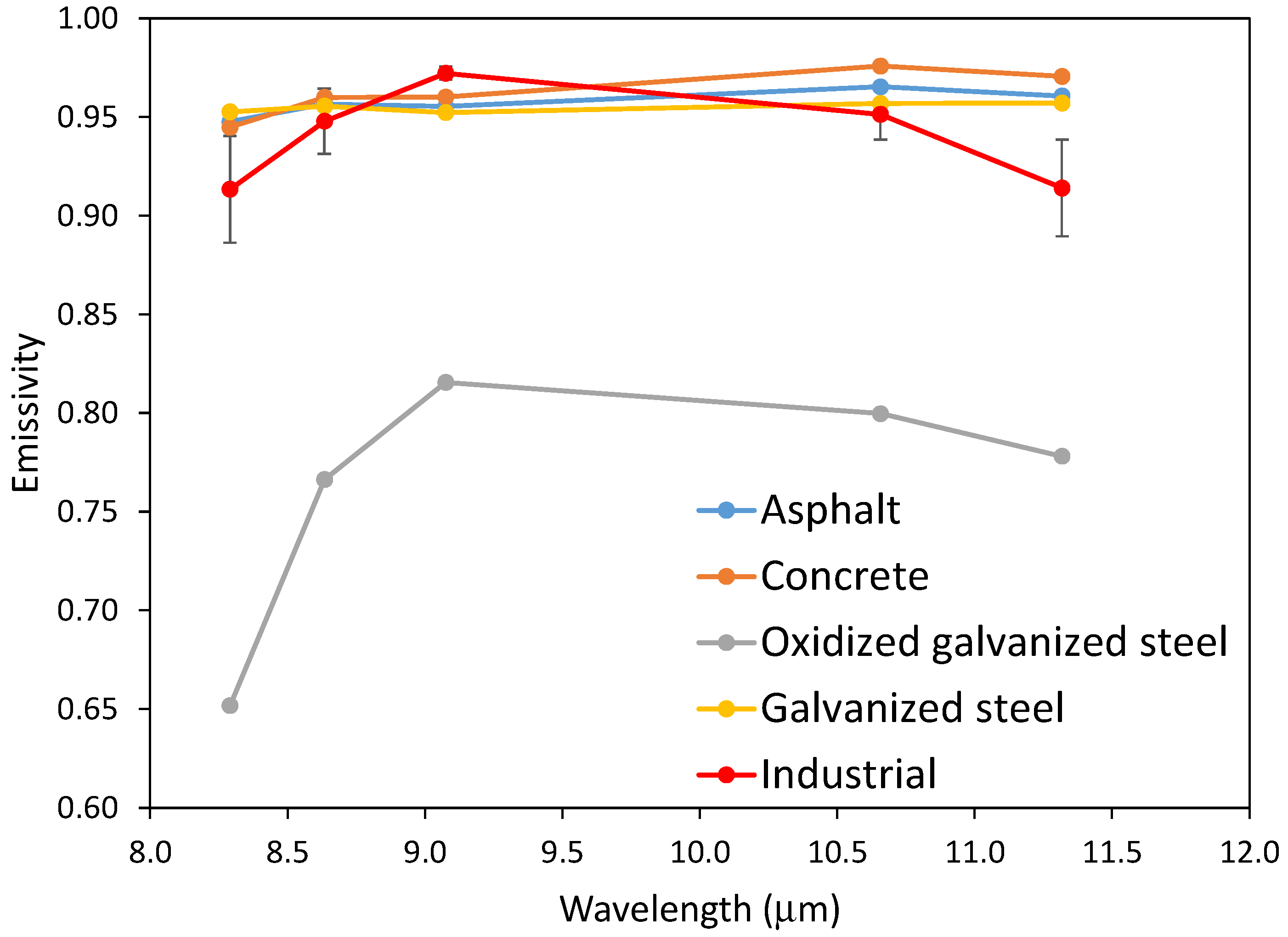
For urban areas, the ASTER library spectra of manmade materials were divided into three groups: construction concrete (to estimate the emissivity of building walls), road asphalts and tars (to estimate the emissivity of streets) and roofing materials (emissivity of building tops). All the spectra in these groups were integrated with the filter functions. For each group, the average and the standard deviation were calculated, obtaining three values of emissivity with a given uncertainty (see

Table 6. Emissivity of urban areas (${\epsilon }_{urbanarea}$) used by the VCM algorithm for the ASTER TIR bands. The values of the emissivities and uncertainties of building tops (${\epsilon }_t$), streets (${\epsilon }_g$) and building walls (${\epsilon }_w$) used to retrieve the emissivity of urban areas are also shown. See the main text for additional details.

ASTER Band	${\mathit{\epsilon }}_{\mathit{g}}$			${\mathit{\epsilon }}_{\mathit{w}}$			${\mathit{\epsilon }}_{\mathit{t}}$			${\mathit{\epsilon }}_{\mathit{urban}\mathit{area}}$
10	0.941	±	0.013	0.92	±	0.03	0.94	±	0.07	0.96	±	0.03
11	0.945	±	0.013	0.92	±	0.03	0.92	±	0.09	0.95	±	0.04
12	0.942	±	0.014	0.90	±	0.04	0.88	±	0.11	0.92	±	0.05
13	0.956	±	0.014	0.96	±	0.02	0.94	±	0.03	0.970	±	0.013
14	0.956	±	0.012	0.959	±	0.007	0.954	±	0.019	0.973	±	0.010

). With these values, the effective emissivity of the urban areas was determined using the model of Caselles and Sobrino described in [39]:

$${\epsilon }_{urbanarea}={\epsilon }_t{P}_t+{\epsilon }_g\left(1-P_t\right)+{\epsilon }_w\left(1-{\epsilon }_g\right)\left(1-P_t\right)\left[\left(1+\frac{H}{S}\right)-\sqrt{1+{\left(\frac{H}{S}\right)}^2}\right]$$

(13)

where ${\epsilon }_t$ is the roofing materials emissivity (building tops), ${\epsilon }_g$ is road asphalts and tars emissivity (streets), ${\epsilon }_w$ is construction concrete emissivity (building walls), $P_t$ is the roof proportion, H is the height of components in the urban area and S is the separation between these components.

In the calculations, different combinations of the aspect ratio H/S (from 0.5–10, at intervals of 0.5) and $P_t$ (from 0.2–0.8, at intervals of 0.05) were considered for the possible urban structures. Using these values, urban emissivity values were simulated using a random procedure considering that the different variables in Equation (13) were normally distributed around a mean value, given by the mean values in Table 6, with a standard deviation given by the corresponding uncertainties in that table. Each simulation in this procedure gives as a result an emissivity for the urban area. The procedure was repeated 25 times, from which the final urban emissivity value was calculated as the average of the 25 different obtained values. It was checked that the use of a larger number of repetitions did not change the obtained average value and the standard deviation. The final values and uncertainties for the urban emissivity at the ASTER bands are shown in Table 6.

In the ANEM algorithm, the VCM emissivity values for the natural areas must be calculated for each scene; however, the estimated values for water and urban areas can be used for every ASTER scene and do not need to be estimated again.

4. Results

4.1. Land Surface Temperature and Emissivity Evaluation

The values retrieved from TES and ANEM algorithms and the ASTER AST08 product were compared with ground measurements at the rice fields around the Albufera Lake and water from the Mediterranean Sea. LST values retrieved with each source are shown in

Table 7. LST values retrieved at evaluation points of rice crops and water from TES, Adjusted Normalized Emissivity Method (ANEM) and AST08 scenes, together with reference values measured at the ground for each analyzed day. The standard deviation (Std) of each measurement is also shown.

	Date	TES		ANEM		AST08		REFERENCE
		LST (K)	Std (K)	LST (K)	Std (K)	LST (K)	Std (K)	LST (K)	Std (K)
RICE	3 August 2004	304.2	0.4	303.8	0.4	304.3	0.3	303.6	0.7
	12 August 2004	302.5	0.5	302.2	0.5	303.0	0.5	302.0	0.5
	21 July 2005	302.5	0.6	302.0	0.5	302.5	0.5	301.6	0.6
	24 July 2006	303.0	0.6	302.5	0.5	304.5	0.5	302.4	0.9
	11 July 2007	301.6	0.6	301.3	0.5	302.6	0.4	300.3	0.3
WATER	3 August 2004	299.3	0.2	298.8	0.1	299.9	0.3	299.3	0.2
	12 August 2004	300.4	0.2	300.1	0.2	301.3	0.3	299.6	0.3
	21 July 2005	300.2	0.3	299.7	0.2	300.9	0.3	299.8	0.2
	24 July 2006	300.7	0.3	300.3	0.2	302.2	0.3	301.0	0.2
	11 July 2007	298.5	0.3	298.1	0.2	299.6	0.3	297.9	0.2

.

From the comparison of LST and SST values in Table 7, a better agreement between ANEM and the reference values is obtained in both areas, rice crops and the Mediterranean Sea. For the rice crops area, the three products overestimate the LST reference value, with a mean bias of +0.8 K for TES, +0.4 K for ANEM and +1.4 K for the AST08 product. While for seawater, the mean bias for TES is +0.3 K, −0.1 K for ANEM and +1.3 K for the AST08 product. In these cases, TES and the AST08 product overestimate the references values while ANEM shows a slight underestimation of them, although on some days, such as 3 August 2004 and 11 July 2007, ANEM overestimates the SST value. It was checked that the standard deviation of SST did not depend significantly on the number of pixels used for the calculation (with similar results for 3 × 3 and 33 × 33 pixel boxes).

The emissivity at the same points was retrieved for the ASTER thermal bands using the TES and ANEM algorithms and also the AST05 product. These emissivity values were compared with the reference measurements for rice crops and water. A comparison for the sand beach was added in this analysis.

The obtained rice crop emissivity spectra corresponding to the days analyzed in this paper are shown in Figure 3. Vertical bar errors depicted in Figure 3 represent the standard deviation of the 3 × 3 window centered on the pixel of the evaluation point.

Results show a better agreement between TES values and the reference for shorter wavelength bands, while for ASTER Bands 13 and 14, ANEM emissivity is closer to the reference values. Average differences between TES, ANEM and AST05 with reference values are, respectively: 0.003, 0.014 and −0.012 for Band 10; −0.003, 0.007 and −0.021 for Band 11; −0.004, 0.006 and −0.027 for Band 12; −0.009, 0.0 and −0.011 for Band 13; and finally, −0.010, 0.0 and −0.014 for Band 14. The underestimated values of TES and AST05 emissivity are in accordance with the LST bias observed before. Moreover, the larger LST difference observed in AST08 is shown again in Figure 3 in terms of emissivity differences in the AST05 product.

In Figure 4, water spectral emissivity is depicted for each studied day. Vertical bar errors in Figure 4 represent the standard deviation of the 33 × 33 window centered on the pixel of the evaluation point.

Results in Figure 4 show better agreement between ANEM and reference emissivity, with differences under 1%. Differences between TES, ANEM and the AST05 product and reference values are, respectively: −0.014, −0.005 and −0.047 for Band 10; −0.016, −0.007 and −0.048 for Band 11; −0.011, −0.002 and −0.049 for Band 12; −0.012, −0.003 and −0.023 for Band 13; and −0.013, −0.004 and −0.026 for Band 14. These results are in accordance with the SST values of Table 7, which determined that the ANEM SST was the most accurate compared to the reference. The largest differences were shown, as with LST, by the AST05 product, with differences up to 5%. It is noticed that all of them underestimate reference emissivity as was observed previously over low-contrast surfaces [21]. This underestimation is more pronounced at Bands 10–12, as was observed in [13].

The emissivity comparison was also made using pixels along the beach coastline, since the sand emissivity spectrum was also measured in situ. In Figure 5, the retrieved emissivity spectra are depicted together with the reference emissivity of sand beach measured using the TES method with the CIMEL 312-2 radiometer.

Results in Figure 5 show a better agreement of the AST05 product, with differences below 1% in some cases with respect to the reference values. Average differences between TES, ANEM and AST05 with reference values are, respectively: 0.063, 0.059 and −0.001 for Band 10; 0.082, 0.083 and 0.037 for Band 11; 0.077, 0.079 and 0.032 for Band 12; 0.011, 0.015 and 0.008 for Band 13; and 0.011, 0.015 and −0.009 for Band 14. For sand, the ASTER product AST05 works better than TES and ANEM, with values closer to the reference. These results show that the ASTER product is working pretty well for this high contrast surface (sand beach), but shows significant errors in relation to low contrast surfaces (i.e., vegetation and water). The atmospherically-adjusted and -recalibrated TES used in this work and the ANEM algorithm supply very similar values in the case of sand, although they are overestimating significantly the emissivity in Channels 10–12, giving better results in Bands 13 and 14.

4.2. Comparison between TES and ANEM

To compare both methods over different surface types, four different cover types characteristic of the area were chosen: rice crop, water, orange fields and urban areas. Emissivity spectra for the four classes are presented in Figure 6, Figure 7, Figure 8 and Figure 9.

Rice crop emissivity for ASTER bands is depicted in Figure 6. This emissivity was calculated as the average value of all pixels classified as rice crop; vertical bar errors show the emissivity standard deviation. These spectra show ANEM emissivities higher than TES ones, with differences ${\epsilon }_{TES}-{\epsilon }_{ANEM}$ ranging between −0.009 and −0.012 depending on the spectral band and the analyzed scene, with larger differences for lower wavelengths. In comparison to the reference spectrum in Figure 3, TES underestimates emissivity, while ANEM overestimates it, but in both cases, the differences are within the measurement errors. As shown in Figure 3, TES adjusted better for lower wavelengths, with differences smaller than ±0.005 in ASTER Bands 10, 11 and 12, while for Bands 13 and 14, these differences are up to ±0.013. For ANEM emissivity, Band 10 shows a difference up to ±0.015; Bands 11 and 12 show differences lower than ±0.008; and for Bands 13 and 14, the emissivity values are closer, with differences below ±0.003. The standard deviation obtained for each channel emissivity is higher for shorter wavelengths than for longer ones, taking values from ±0.006–±0.013 for TES and from ±0.004–±0.011 for ANEM, showing a reasonable homogeneity within this class.

The same analysis was performed for pixels classified as water, which include the Mediterranean Sea and the Albufera Lake, and the results are shown in Figure 7. ANEM produces emissivity values higher than TES. There is a constant difference between them for all bands of ${\epsilon }_{TES}-{\epsilon }_{ANEM}=-0.009$, which means a consistency in the spectral shape retrieved from both methods. This shape is in accordance with the reference spectra shown in Figure 4, although both methods underestimated the reference values, with higher differences for TES, which are up to −0.022, than for ANEM with differences up to −0.011. The standard deviations depicted with the error bars present values between ±0.004 and ±0.015 for TES and between ±0.003 and ±0.012 for ANEM, showing lower deviations for Bands 13 and 14 and higher for Bands 10 and 11.

Since the agricultural area is the most extensive class, an orange field area common for the five scenes was selected to provide a surface with constant vegetation fractional cover over time (trees are green-leaved and have no fruits in the summer season). Figure 8 shows the emissivity spectra for this class. For each scene, the TES and ANEM methods provide the same spectral shape for each day, with emissivity differences ${\epsilon }_{TES}-{\epsilon }_{ANEM}$ of −0.010 for 3 August 2004, −0.009 for 12 August 2004, −0.014 for 21 July 2005 and 24 July 2006 and −0.011 for 11 July 2007. The standard deviation for TES ranges between ±0.004 and ±0.012, and for ANEM, it does between ±0.003 and ±0.010.

Figure 9 shows the emissivity corresponding to urban areas, which include cities, towns, industrial zones and other urbanized sites. For urban surfaces, emissivity spectra retrieved from TES and ANEM provide closer values, with differences below ±0.004. For ASTER Bands 10, 11 and 12, TES overestimates ANEM values, with differences ${\epsilon }_{TES}-{\epsilon }_{ANEM}$ up to +0.007. For Bands 13 and 14, it depends on the scene, but the differences are very close to zero. The standard deviation obtained for TES is between ±0.009 and ±0.018, and for ANEM, it is between ±0.008 and ±0.020, with higher differences for lower wavelengths.

5. Discussion

5.1. Advantages and Limitations of TES and ANEM

TES and ANEM algorithms have as a common point the use of the NEM method. TES uses NEM as the initial module starting from a single emissivity value for every pixel and channel to get a first-guess relative spectrum, which is then spectrally tuned using the MMD empirical relationship getting finally the LST. ANEM obtains a maximum emissivity value different for each pixel (contrary to TES) using the VCM algorithm, then obtains the emissivity spectrum using this first-guess emissivity in the NEM method.

Both methods need the use of at-surface radiances corrected for the atmospheric effects as input data. For this reason, atmospheric correction with radiosounding profiles spatially and temporally coincident to the ASTER data recordings and local recalibration of the ASTER radiances were used. This procedure assured that both methods were compared under optimal conditions.

A rough classification is required in the VCM module of ANEM to separate the vegetated surfaces from urban and water areas (and eventually, ice/snow where needed). For water and urban areas, the maximum emissivity is estimated once (as in this paper) and can be applied to different scenes and areas. For the vegetated surface, the maximum emissivity for NEM needs an estimation of the fractional vegetation cover that can be calculated easily from VNIR data using the proposed methodology with low dependence on the atmospheric correction and two average emissivity coefficients, namely bare soil and vegetation emissivity. A mean emissivity is enough for vegetation, but it could be insufficient to describe the variation of all soil types, especially in the 8–10-µm range. However, the soil emissivity usually peaks within 10–12 µm just where soil emissivities show much lower variability as can be seen in the standard deviation of the soil coefficients for ASTER Channels 13 and 14 in Table 5 (below ±0.006). Note that in ANEM, the VCM is used to get a first-guess maximum emissivity as the input to the NEM module and not to obtain the final spectrum. In addition, the VCM allows adjusting this first-guess considering the temporal changes in the surface introduced by the vegetation phenology; these changes can be significant through the year especially for senescent vegetation and agricultural areas.

The matrix confusion of the classification was used to check its accuracy, and it showed an overall accuracy of 97.3% and an index kappa of 0.967. In any case, an estimation of the emissivity error in ANEM due to misclassified pixels was also made. It would cause a difference in the initial emissivity at the NEM module. If a pixel of the urban area were misclassified as water or vegetated area, or vice versa, this difference in the initial emissivity would be ±0.015. This difference at the initial emissivity would lead to errors up to ±0.7 K in the final LST following the described methodology.

In contrast, TES applies the NEM module with a single emissivity value to get a first relative emissivity spectrum and LST value. They are then refined by using the MMD empirical relationship that places the absolute value of the emissivity spectrum providing the final LST. The main drawback of TES is the MMD relationship that was initially derived with a strong predominance of soil and rock samples, although it was modified by Hulley and Hook in [12] by adding simulated samples with different degrees of vegetation cover; and the high sensitivity of the MMD to residual errors in the atmospheric correction that makes this relationship provide too low minimum emissivities, thus lowering the whole spectrum. For that reason, TES provides in general excellent results over high contrast surfaces (almost all the validation exercises have been conducted till present over desert areas), but more modest results over vegetated or water surfaces.

5.2. Quality of Reference Data

Different data were used as the reference for validating the results obtained. For rice crops, LST data were measured with several CIMEL 312 radiometers deployed in the field concurrent to the scene acquisition, providing accurate ground reference values. For water, no radiometric or contact temperatures provided by sea buoys were available at the time of scene acquisitions; thus, the MODIS L2 SST product (MOD28) was taken as the reference, or at least as a cross-comparison for the TES and ANEM results. Although the MOD28 SST product is not a ground reference strictly speaking, the SST values are obtained using a split-window algorithm devised specifically for the sea surface and has been extensively validated [40,41,42,43], in particular including buoys in the Mediterranean Sea in the comparison [34], providing an overall accuracy of ±0.37 K (for MODIS viewing angles ≤40°) that gives confidence to these data as a valid reference for TES and ANEM. The difference in spatial resolution of MODIS (1 km) and ASTER (90 m) is not a limiting condition for the comparison, since SST usually varies smoothly in space as can be seen in the low standard deviations of the MODIS SST data collected in 3 × 3 pixel boxes (<0.2 K) and the corresponding TES and ANEM SST values for 33 × 33 pixel windows (<0.3 K).

5.3. LSE and LST Evaluation

With regard to the LST evaluation using the reference measurements, the ASTER AST08 product retrieved values within the uncertainty established in [10], as other previous works have pointed out [13,22]. However, the LSTs obtained from the applied TES and ANEM algorithms showed a better accuracy in this paper when applied to data with a more site-specific atmospheric correction, the results being slightly better for ANEM than for TES.

With regard to emissivity, it is observed that for surfaces with low spectral contrast such as water or rice crops, AST05 provides less accurate values than ANEM or TES out of the predicted uncertainty range proposed in [10]. These differences could be due to the empirical expression to retrieve the minimum emissivity from MMD at the AST05 product algorithm, which is not fitted to low contrast surfaces [12], as well as to the atmospheric correction applied at the product AST05, since NCEP atmospheric profiles are less accurate than profiles obtained by in situ radiosoundings [44,45]. As an example, Pérez-Planells et al. in [45] showed that using interpolated NCEP profiles instead of radiosoundings yielded errors of ±0.6 K for sites close to sea level, which would be equivalent to ±0.01 in terms of emissivity. Moreover, previous studies pointed out that ASTER product atmospheric correction loses accuracy in warm and humid areas close to sea level [23,24]. Despite using an MMD relationship including additional samples for vegetated surfaces and a local recalibration and atmospheric correction, the results of emissivity for these surfaces are systematically lower for TES than for ANEM (see Figure 3 and Figure 4), which confirms the existence of an impact of residual atmospheric correction errors that may be affecting TES emissivities more than ANEM ones.

Nevertheless, for a high contrast surface as the sand beach is, the AST05 product fits much better to the ground reference measurement than the TES applied in this paper and ANEM, especially for spectral bands from 8–10 µm. It is difficult to find an explanation of this result, provided that the AST05 product and the TES version applied in this work should at least give similar results, since a local radiosounding was used in the latter. By contrast, TES provides virtually the same results as ANEM for that surface type.

5.4. TES and ANEM Comparison over Time

The comparison between TES and ANEM algorithms on different surfaces over time shows that the obtained spectra are consistent for all surfaces, with little differences, which are always within the uncertainty. For rice crop, water and orange field, ANEM emissivity values are higher than TES by 1%, ANEM results being closer to the ground reference values.

For urban areas, an overestimation of TES emissivity is observed, which does not appear in the previous classes, so urban area is a class that provides pixels with positive differences between TES and ANEM. In this class, moreover, the spectra show again temporal consistency over the years, as was the case of rice crops and water.

It is worth showing that two different areas can be distinguished inside the urban class. Using TES emissivities in ASTER Bands 10, 12 and 14, emissivity bands in the RGB composition shown in Figure 10 for the scene on 3 August 2004, city areas (red pixels) can be clearly distinguished from industrial areas (green pixels); a difference that cannot be clearly observed with the VNIR and SWIR bands. The same effect was observed using ANEM emissivities. For each scene, a set of 3 × 3 pixels (selected from visual inspection of Figure 10) was used to retrieve the emissivity spectra of each area for the five TES scenes used in this work, obtaining the results shown in Figure 11.

A clearly different spectrum for each area is observed. The main construction materials for the city area are red bricks, terra cotta tiles and asphalt for building roofing and streets. The emissivity spectra of these materials were retrieved from the ASTER Spectral Library and integrated for the TIR ASTER bands (see Figure 12). The same process was done for the industrial area, considering concrete, galvanized steel, oxidized galvanized steel and asphalt as the main construction materials for this area (see Figure 13). Oxidized galvanized steel was also included because galvanized steel oxidizes after a time outdoors.

The TES emissivity spectra obtained for the city area (Figure 11) resemble the spectra of red brick and asphalt roofing (Figure 12), showing similar shapes. This is reasonable, since red brick is one of the materials most used in buildings. It is observed that the city spectra show values higher than any material; this may be due to the cavity effect caused by the city structure. Looking at the industrial area, the TES emissivity spectra shown in Figure 11 are very similar to the shape of the oxidized galvanized steel spectrum shown in Figure 13. It should be noted that this last spectrum does not fit the MMD regression curve used by TES, showing lower values (${\epsilon }_{min}$ = 0.65) than those predicted by Equation (7) (${\epsilon }_{min}$ = 0.82) for MMD = 0.16 observed in Figure 13. Taking into account the spectra of the other materials used in these zones, which have higher emissivity values and a lower spectral contrast, and taking into account the cavity effect, the spectra compare reasonably well.

6. Conclusions

This paper compared the TES and ANEM algorithms using L1 ASTER data that were recalibrated and atmospherically corrected using concurrent local atmospheric profiles. The algorithms were applied to a set of five ASTER scenes over the area of Valencia, Spain, which included water, agricultural and urban areas. The results were compared to the ASTER temperature and emissivity standard products (AST08 and AST05 products, respectively).

The surface temperatures obtained from TES, ANEM and AST08 product were validated with reference measurements taken on a rice paddy located near the Albufera Lake of Valencia and also with the sea surface temperature provided by Terra MODIS (MOD28 product). From these comparisons, it is concluded that ANEM shows the best agreement, with a bias of +0.4 K and −0.01 K for LST and SST, respectively. For TES, biases are +0.8 K and +0.3 K, respectively. Both methods provide good results since their accuracy is less than 1 K. Results shown by the AST08 product are worse, with biases of +1.4 K for LST and +1.3 K for SST; this may be due largely to the use of NCEP profiles for atmospheric correction in AST08 in comparison to the local recalibration and atmospheric correction performed in ANEM and TES.

The emissivity spectra obtained with both methods and provided by the AST05 product were compared on two land surfaces, rice and sand, for which ground measurements were made, and on the sea surface using the water spectra provided by the ASTER spectral library. It was observed that in the case of rice crops, TES provided values closer to the reference spectra in ASTER Bands 10–12, while ANEM showed better accuracy for ASTER Bands 13 and 14. For water, both the TES and ANEM methods underestimated the emissivity. ANEM results were closer to the reference with differences lower than 0.005, while for TES, these differences were up to 0.015. In comparison, the AST05 product showed less agreement in these two low-contrast surfaces, yielding differences up to −0.027 for rice crops and −0.050 for water. For sand, differences between TES and ANEM were less than 0.005, and they disagreed with the reference measurement by 0.06–0.08 for Bands 10–12 and by 0.011–0.015 for Bands 13 and 14. In contrast, the results shown by the AST05 product in this case were much better, showing biases of −0.001 for Band 10, +0.037 for Band 11, +0.032 for Band 12, +0.008 for Band 13 and −0.009 for Band 14. These were out of the uncertainty predicted for the AST05 product, which could be attributed to residual errors in the atmospheric correction used in the ASTER products, as has been pointed out previously [21,23,25], as well as to the deficient adjustment for low-contrast surfaces in the MMD empirical relationship [21]. However, results showed a better agreement of the AST05 product over high spectral contrast areas, such as a sandy beach.

The TES and ANEM results were also compared to each other using four known surface types common for the scenes. For surfaces with low spectral contrast, such as water or vegetated areas, ANEM systematically overestimated TES emissivity, yielding closer values to the reference emissivity. However, for surfaces with a high spectral difference, such as urban areas, ANEM obtained values lower than TES, but close to them. Both methods were capable of separating surfaces with different spectral behaviors, as shown in the analysis of the urban areas. In addition, the temporal evolution of the obtained emissivity spectra in both cases could be used to monitor changes in the observed surfaces as has been also indicated by Hulley et al. in [46].

Future work will be addressed to analyzing the use of more efficient atmospheric correction algorithms in TES and ANEM, such as the Water Vapor Scaling (WVS) method [24] or the Single-Band Atmospheric Correction (SBAC) [47], and the eventual combination of TES and ANEM in a single algorithm that could benefit from the strengths shown by both methods.

References

1. Zhang, R.; Tian, J.; Su, H.; Sun, X.; Chen, S.; Xia, J. Two improvements of an operational two-layer model for terrestrial surface heat flux retrieval. Sensors 2008, 8, 6165–6187. [Google Scholar] [CrossRef] [PubMed]
2. Anderson, M.C.; Kustas, W.P.; Norman, J.M.; Hain, C.R.; Mecikalski, J.R.; Schultz, L.; González-Dugo, M.P.; Cammalleri, C.; D’Urso, G.; Pimstein, A.; et al. Mapping daily evapotranspiration at field to continental scales using geostationary and polar orbiting satellite imagery. Hydrol. Earth Syst. Sci. 2011, 15, 223–239. [Google Scholar] [CrossRef] [Green Version]
3. Sánchez, J.M.; López-Urrea, R.; Rubio, E.; González-Piqueras, J.; Caselles, V. Assessing crop coefficients of sunflower and canola using two-source energy balance and thermal radiometry. Agric. Water Manag. 2014, 137, 23–29. [Google Scholar] [CrossRef]
4. Li, Z.; Tang, B.; Wu, H.; Ren, H.; Yan, G.; Wan, Z.; Trigo, I.F.; Sobrino, J.A. Satellite-derived land surface temperature: Current status and perspectives. Remote Sens. Environ. 2013, 131, 14–37. [Google Scholar] [CrossRef]
5. Watson, K. Two-temperature method for measuring emissivity. Remote Sens. Environ. 1992, 42, 117–121. [Google Scholar] [CrossRef]
6. Li, Z.L.; Becker, F. Feasibility of land surface temperature and emissivity determination from AVHRR data. Remote Sens. Environ. 1993, 43, 67–85. [Google Scholar] [CrossRef]
7. Barducci, A.; Pippi, I. Temperature and emissivity retrieval from remotely sensed images using the “grey body emissivity” method. IEEE Trans. Geosci. Remote Sens. 1996, 34, 681–695. [Google Scholar] [CrossRef]
8. Borel, C. Iterative Retrieval of Surface Emissivity and Temperature for a Hyperspectral Sensor. In Proceedings of the 1st JPL Workshop on Remote Sensing of Land Surface Emissivity, Pasadena, CA, USA, 6–8 May 1997. [Google Scholar]
9. Wan, Z.; Li, Z.L. A physics-based algorithm for retrieving land-surface emissivity and temperature from eos/modis data. IEEE Trans. Geosci. Remote Sens. 1997, 35, 980–996. [Google Scholar]
10. Gillespie, A.; Rokugawa, S.; Matsunaga, T.; Cothern, J.S.; Hook, S.; Kahle, A.B. A Temperature and Emissivity Separation Algorithm for Advanced Spaceborne Thermal Emission and Reflection Radiometer (ASTER) Images. IEEE Trans. Geosci. Remote Sens. 1998, 36, 1113–1126. [Google Scholar] [CrossRef]
11. Wang, N.; Wu, H.; Nerry, F.; Li, C.; Li, Z.L. Temperature and emissivity retrievals from hyperspectral thermal infrared data using linear spectral emissivity constraint. IEEE Trans. Geosci. Remote Sens. 2011, 49, 1291–1303. [Google Scholar] [CrossRef]
12. Hulley, G.C.; Hook, S.J. The North American ASTER Land Surface Emissivity Database (NAALSED) Version 2.0. Remote Sens. Environ. 2009, 113, 1967–1975. [Google Scholar] [CrossRef]
13. Sabol, D.E.; Gillespie, A.R.; Abbott, E.; Yamada, G. Field validation of the ASTER Temperature-Emissivity Separation algorithm. Remote Sens. Environ. 2009, 113, 2328–2344. [Google Scholar] [CrossRef]
14. Jiménez-muñoz, J.C.; Sobrino, J.A.; Mattar, C.; Hulley, G.; Göttsche, F. Temperature and Emissivity Separation from MSG/SEVIRI Data. IEEE Trans. Geosci. Remote Sens. 2013, 52, 1–15. [Google Scholar] [CrossRef]
15. Coll, C.; García-Santos, V.; Niclòs, R.; Caselles, V. Test of the MODIS Land Surface Temperature and Emissivity Separation Algorithm with ground measurements over a rice paddy. IEEE Trans. Geosci. Remote Sens. 2016, 54, 3061–3069. [Google Scholar] [CrossRef]
16. Islam, T.; Hulley, G.; Malakar, N.; Radocinski, R.; Guillevic, P.; Hook, S. A physics-based algorithm for the simultaneous retrieval of land surface temperature and emissivity from VIIRS thermal infrared data. IEEE Trans. Geosci. Remote Sens. 2017, 55, 563–576. [Google Scholar] [CrossRef]
17. Coll, C.; Caselles, V.; Rubio, E.; Sospedra, F.; Valor, E. Temperature and emissivity separation from calibrated data of the Digital Airborne Imaging Spectrometer. Remote Sens. Environ. 2001, 76, 250–259. [Google Scholar] [CrossRef]
18. Coll, C.; Valor, E.; Caselles, V.; Niclo, R. Adjusted Normalized Emissivity Method for surface temperature and emissivity retrieval from optical and thermal infrared remote sensing data. J. Geophys. Res. 2003, 108, 1–14. [Google Scholar] [CrossRef]
19. Gillespie, A.R. Lithologic Mapping of Silicate Rocks Using TIMS; TIMS Data User’s Workshop Jet Propulsion Laboratory: Pasadena, CA, USA, 1986; pp. 29–44. [Google Scholar]
20. Valor, E.; Caselles, V. Mapping Land Surface Emissivity from NDVI: Application to European, African, and South American Areas. Remote Sens. Environ. 1996, 184, 167–184. [Google Scholar] [CrossRef]
21. Coll, C.; Caselles, V.; Valor, E.; Niclòs, R.; Sánchez, J.M.; Galve, J.M.; Mira, M. Temperature and emissivity separation from ASTER data for low spectral contrast surfaces. Remote Sens. Environ. 2007, 110, 162–175. [Google Scholar] [CrossRef]
22. Barreto, Á.; Arbelo, M.; Hernández-Leal, P.A.; Núez-Casillas, L.; Mira, M.; Coll, C. Evaluation of surface temperature and emissivity derived from ASTER data: A case study using ground-based measurements at a volcanic site. J. Atmos. Ocean. Technol. 2010, 27, 1677–1688. [Google Scholar] [CrossRef]
23. Gillespie, A.R.; Abbott, E.A.; Gilson, L.; Hulley, G.; Jiménez-Muñoz, J.C.; Sobrino, J.A. Residual errors in ASTER temperature and emissivity standard products AST08 and AST05. Remote Sens. Environ. 2011, 115, 3681–3694. [Google Scholar] [CrossRef]
24. Tonooka, H. Accurate atmospheric correction of ASTER thermal infrared imagery using the WVS method. IEEE Trans. Geosci. Remote Sens. 2005, 43, 2778–2792. [Google Scholar] [CrossRef]
25. Gustafson, W.; Gillespie, A.; Yamada, G. Revisions to the ASTER temperature/emissivity separation algorithm. In Proceedings of the 2nd Recent Advances in Quantitative Remote Sensing, Torrent, Spain, 25–29 September 2006; pp. 770–775. [Google Scholar]
26. Chavez, P.S. Image-Based Atmospheric Corrections—Revisited and Improved. Photogramm. Eng. Remote Sens. 1996, 62, 1025–1036. [Google Scholar]
27. Berk, A.; Anderson, G.P.; Acharya, P.K.; Chetwynd, J.H.; Bernstein, L.S.; Shettle, E.P.; Matthew, M.W. MODTRAN4 User’s Manual; Air Force Research Laboratory: Hanscom AFB, Bedford, MA, USA, 1999. [Google Scholar]
28. Gillespie, A.R.; Rokugawa, S.; Hook, S.J.; Matsunaga, T.; Kahle, A.B. Temperature/Emissivity Separation Algorithm Theoretical Basis Document, Version 2.4; NASA: Washington, DC, USA, 1999; Volume 4, pp. 1–64.
29. Thome, K.; Palluconi, F.; Takashima, T.; Masuda, K. Atmospheric correction of ASTER. IEEE Trans. Geosci. Remote Sens. 1998, 36, 1199–1211. [Google Scholar] [CrossRef]
30. Niclòs, R.; Doña, C.; Valor, E.; Bisquert, M.; Niclòs, R.; Doña, C.; Valor, E.; Bisquert, M. Thermal-Infrared Spectral and Angular Characterization of Crude Oil and Seawater Emissivities for Oil Slick Identification. IEEE Trans. Geosci. Remote Sens. 2014, 52, 5387–5395. [Google Scholar]
31. Legrand, M.; Pietras, C.; Brogniez, G.; Haeffelin, M.; Abuhassan, N.K.; Sicard, M. A high-accuracy multiwavelength radiometer for in situ measurements in the thermal infrared. Part I: Characterization of the instrument. J. Atmos. Ocean. Technol. 2000, 17, 1203–1214. [Google Scholar] [CrossRef]
32. Payan, V.; Royer, A. Analysis of Temperature Emissivity Separation (TES) algorithm applicability and sensitivity. Int. J. Remote Sens. 2004, 25, 15–37. [Google Scholar] [CrossRef]
33. Brown, O.B.; Minnett, P.J. MODIS Infrared Sea Surface Temperature Algorithm Algorithm Theoretical Basis Document; University of Miami: Miami, FL, USA, 1999. [Google Scholar]
34. Niclòs, R.; Caselles, V.; Coll, C.; Valor, E. Determination of sea surface temperature at large observation angles using an angular and emissivity-dependent split-window equation. Remote Sens. Environ. 2007, 111, 107–121. [Google Scholar] [CrossRef]
35. Baldridge, A.M.; Hook, S.J.; Grove, C.I.; Rivera, G. The ASTER spectral library version 2.0. Remote Sens. Environ. 2009, 113, 711–715. [Google Scholar] [CrossRef]
36. Caselles, E.; Valor, E.; Abad, F.; Caselles, V. Automatic classification-based generation of thermal infrared land surface emissivity maps using AATSR data over Europe. Remote Sens. Environ. 2012, 124, 321–333. [Google Scholar] [CrossRef]
37. Valor, E.; Caselles, V. Validation of the vegetation cover method for land surface emissivity estimation. In Recent Research Developments in Thermal Remote Sensing; Research Signpost: Kerala, India, 2005. [Google Scholar]
38. Rouse, J.W.; Haas, R.H.; Schell, J.A.; Deering, D.W.; Harlan, J.C. Monitoring the Vernal Advancement and Retrogradation (Greenwave Effect) of Natural Vegetation; Type III, Final Report; NASA/GSFC: Greenbelt, MD, USA, 1974; p. 371.
39. Caselles, V.; Sobrino, J.A. Determination of frost in orange groves from NOAA-9 AVHRR data. Remote Sens. Environ. 1989, 29, 135–146. [Google Scholar] [CrossRef]
40. Marcello, J.; Eugenio, F.; Hernandez, A. Validation of MODIS and AVHRR/3 Sea Surface Temperature Retrieval Algorithms. In Proceedings of the IEEE International Geoscience and Remote Sensing Symposium (IGARSS ’04), Anchorage, AK, USA, 20–24 September 2004; pp. 839–842. [Google Scholar]
41. Lee, M.-A.; Tzeng, M.-T.; Hosoda, K.; Sakaida, F.; Kawamura, H.; Shieh, W.; Yang, Y.; Chang, Y. Validation of JAXA/MODIS Sea Surface Temperature in Water around Taiwan Using the Terra and Aqua Satellites. Terr. Atmos. Ocean. Sci. 2010, 21, 727–736. [Google Scholar] [CrossRef]
42. Qin, H.; Chen, G.; Wang, W.; Wang, D.; Zeng, L. Validation and application of MODIS-derived SST in the South China Sea. Int. J. Remote Sens. 2014, 35, 4315–4328. [Google Scholar] [CrossRef]
43. Hao, Y.; Cui, T.; Singh, V.P.; Zhang, J.; Yu, R.; Zhilei, Z. Validation of MODIS Sea Surface Temperature Product in the Coastal Waters of the Yellow Sea. IEEE J. Sel. Top. Appl. Earth Obs. Remote Sens. 2017, 10, 1667–1680. [Google Scholar] [CrossRef]
44. Coll, C.; Caselles, V.; Valor, E.; Niclòs, R. Comparison between different sources of atmospheric profiles for LST retrieval from single channel thermal infrared data. Remote Sens. Environ. 2012, 117, 199–210. [Google Scholar] [CrossRef]
45. Pérez-Planells, L.; García-Santos, V.; Caselles, V. Comparing different profiles to characterize the atmosphere for three MODIS TIR bands. Atmos. Res. 2015, 161–162, 108–115. [Google Scholar] [CrossRef]
46. Hulley, G.; Veraverbeke, S.; Hook, S. Thermal-based techniques for land cover change detection using a new dynamic MODIS multispectral emissivity product (MOD21). Remote Sens. Environ. 2014, 140, 755–765. [Google Scholar] [CrossRef]
47. Galve, J.M.; Coll, C.; Sánchez, J.M.; Valor, E.; Niclòs, R.; Pérez-Planells, L.; Doña, C.; Caselles, V. Single band atmospheric correction tool for thermal infrared data: Application to Landsat 7 ETM+. In Proceedings of the SPIE 10004, Image and Signal Processing for Remote Sensing XXII, Edinburgh, UK, 26–29 September 2016. [Google Scholar] [CrossRef]
Figure 1. Scene over the study area on 3 August 2004 using VNIR ASTER Channels 3n (0.81 µm), 2 (0.66 µm) and 1 (0.56 µm) to compose the RGB image, respectively.
Remotesensing 09 01251 g001
Figure 2. Difference between minimum emissivity retrieved using the empirical expression proposed in [12] and the one proposed in [10] depending on the maximum-minimum difference (MMD).
Remotesensing 09 01251 g002
Figure 3. Rice crop emissivity for each studied day measured in the field (REFERENCE), obtained with TES and ANEM methods, and provided by the standard product AST05.
Remotesensing 09 01251 g003
Figure 4. Water emissivity for each studied day provided by Niclòs et al. in [34] (REFERENCE), obtained with TES and ANEM methods and provided by the standard product AST05.
Remotesensing 09 01251 g004
Figure 5. Sand emissivity spectra retrieved with the different methods compared to the ground reference measurements carried out on the sand beach.
Remotesensing 09 01251 g005
Figure 6. Mean emissivity retrieved with TES and ANEM methods using the pixels classified as rice crop for the five thermal ASTER bands.
Remotesensing 09 01251 g006
Figure 7. Mean emissivity retrieved with TES and ANEM methods using the pixels classified as water for the five thermal ASTER bands.
Remotesensing 09 01251 g007
Figure 8. Mean emissivity retrieved with TES and ANEM methods using the pixels selected over orange fields for the five thermal ASTER bands.
Remotesensing 09 01251 g008
Figure 9. Mean emissivity retrieved with TES and ANEM methods using the pixels classified as urban area for the five thermal ASTER bands.
Remotesensing 09 01251 g009
Figure 10. Scene over the study area on 3 August 2004 using TES emissivity from ASTER Channels 10 (8.29 µm), 12 (9.08 µm) and 14 (11.32 µm) to compose the RGB image, respectively.
Remotesensing 09 01251 g010
Figure 11. Mean emissivity retrieved with the TES method in 3 × 3 windows over the industrial area (centered on coordinates: 39°14’1’’N 0°29′25″W) and the urban area (centered on coordinates: 39°11′35″N 0°26′2″W) for the five thermal ASTER bands.
Remotesensing 09 01251 g011
Figure 12. Mean emissivity of urban construction materials retrieved from the ASTER Spectral Library and integrated for the five thermal ASTER bands.
Remotesensing 09 01251 g012
Figure 13. Mean emissivity of industrial construction materials retrieved from the ASTER Spectral Library and integrated for the five thermal ASTER bands.
Remotesensing 09 01251 g013