An Analysis of Ku-Band Profiling Radar Observations of Boreal Forest


 ,
,  , , , ,
Abstract
:
1. Introduction
2. Materials and Methods
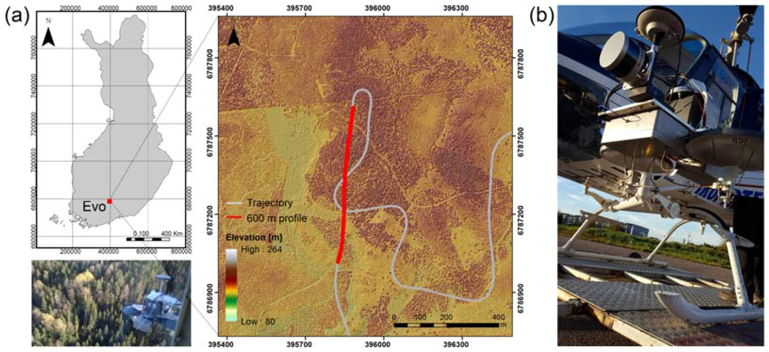
2.1. Study Site
2.2. Tomoradar Data
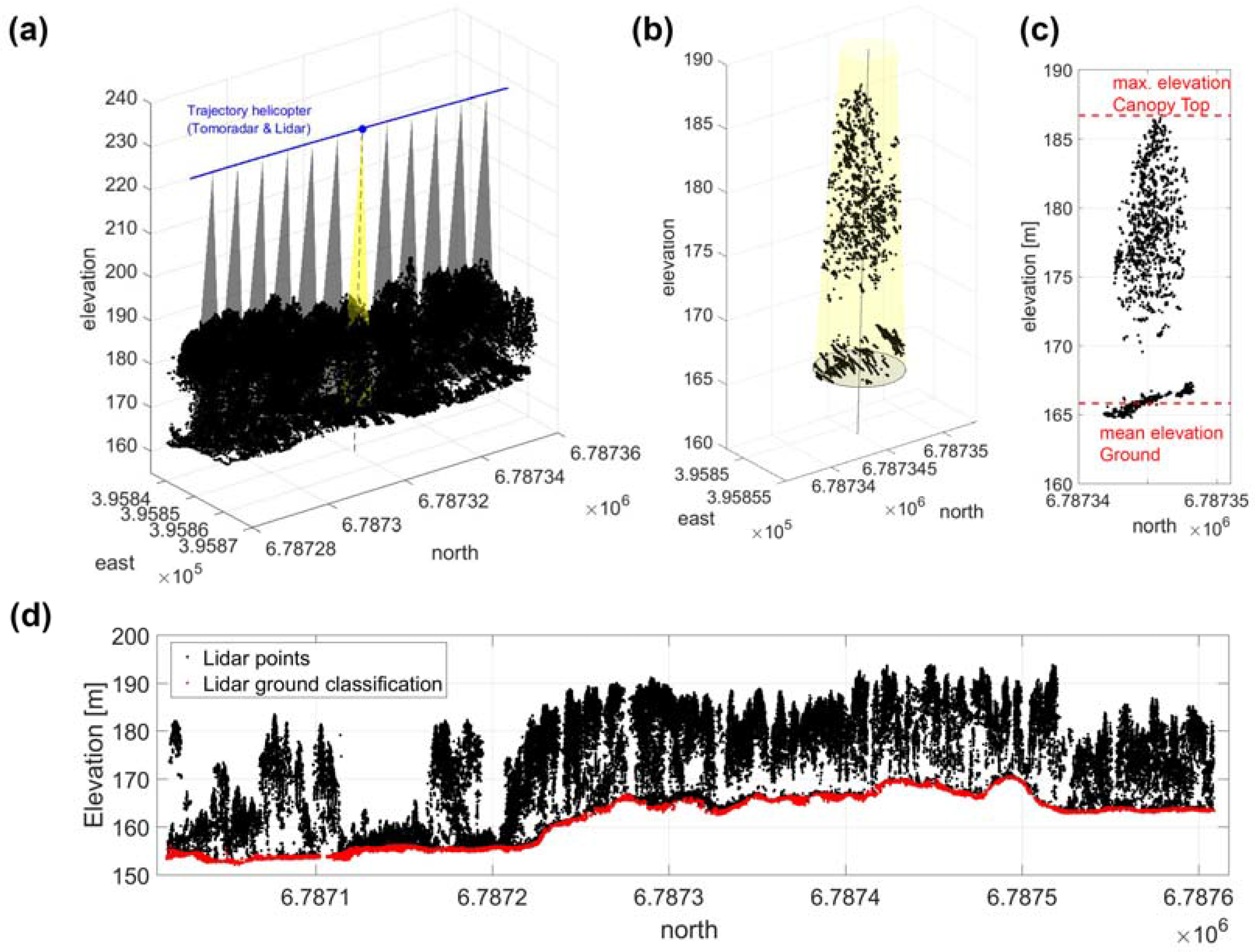
2.3. Lidar Data
2.4. Analyses
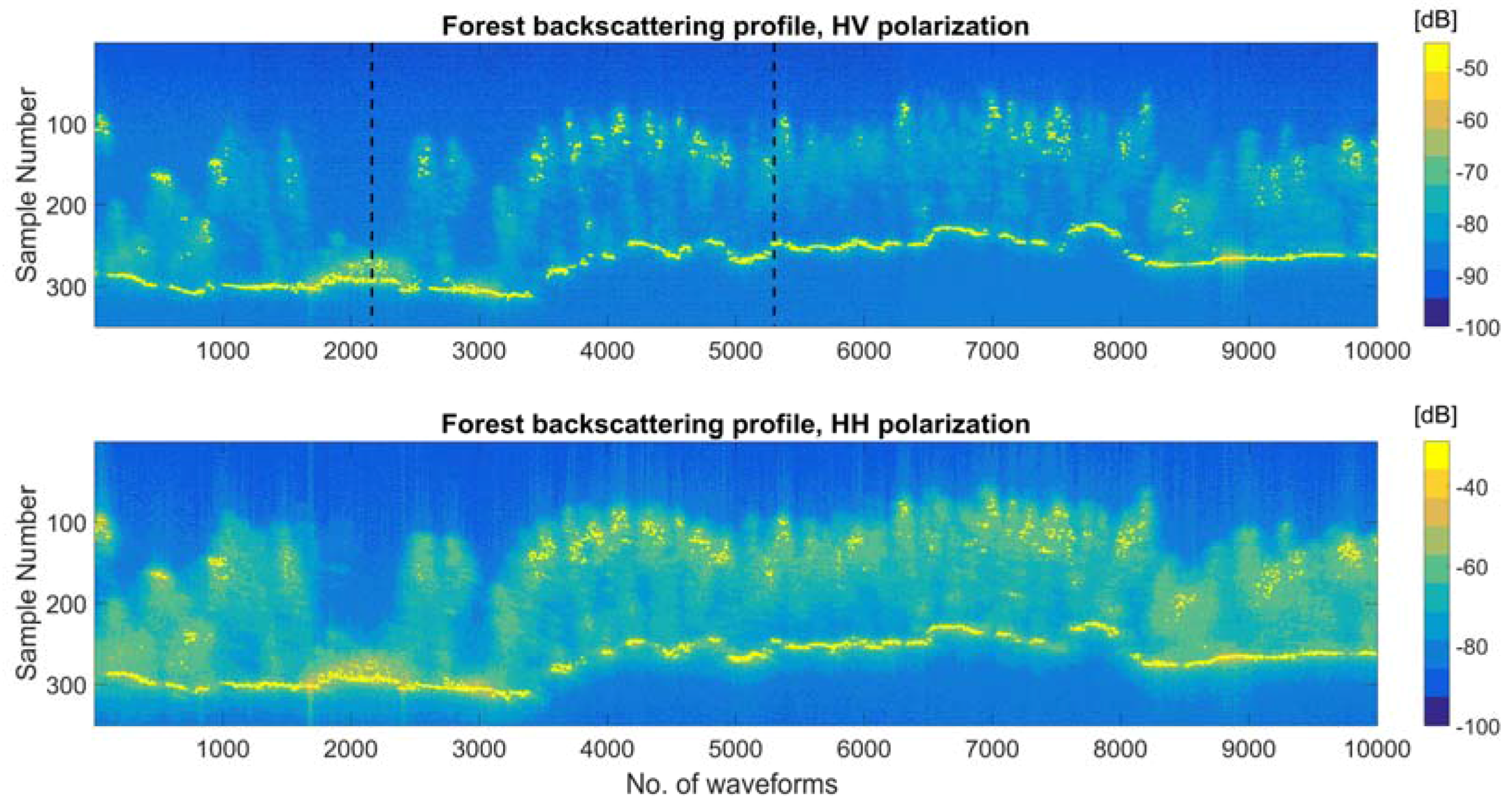
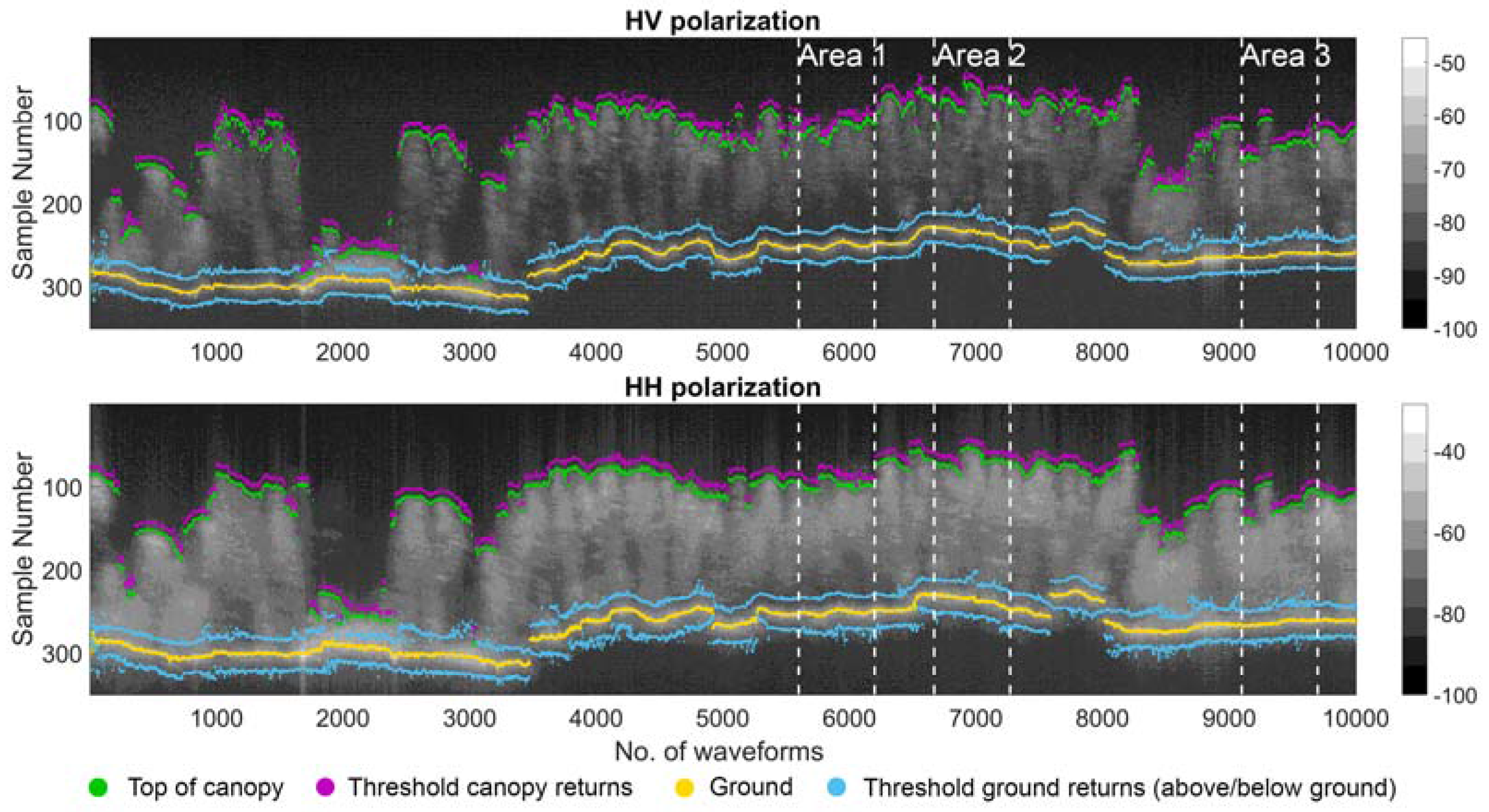
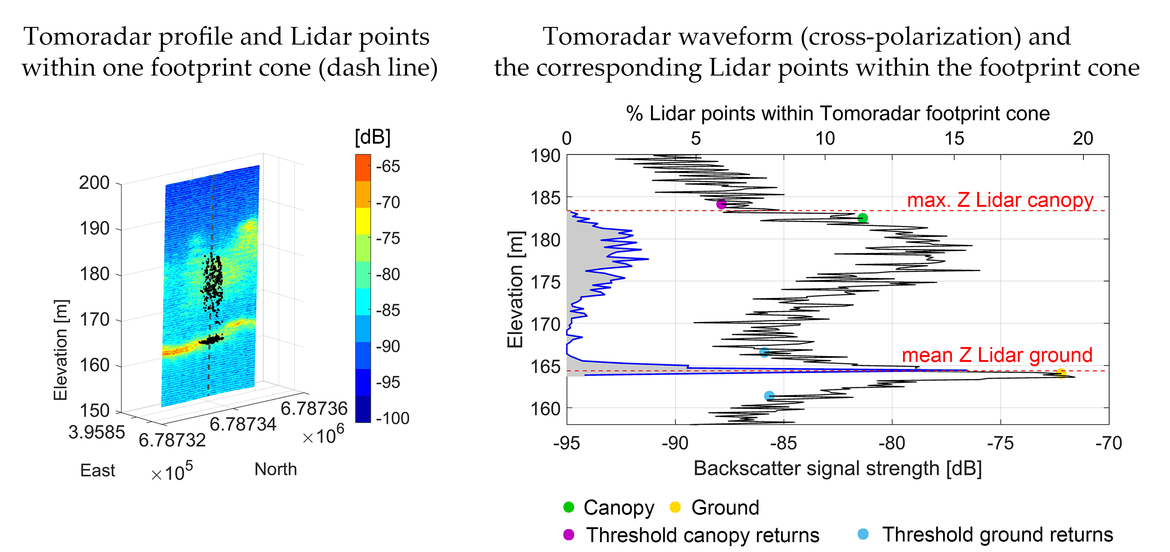
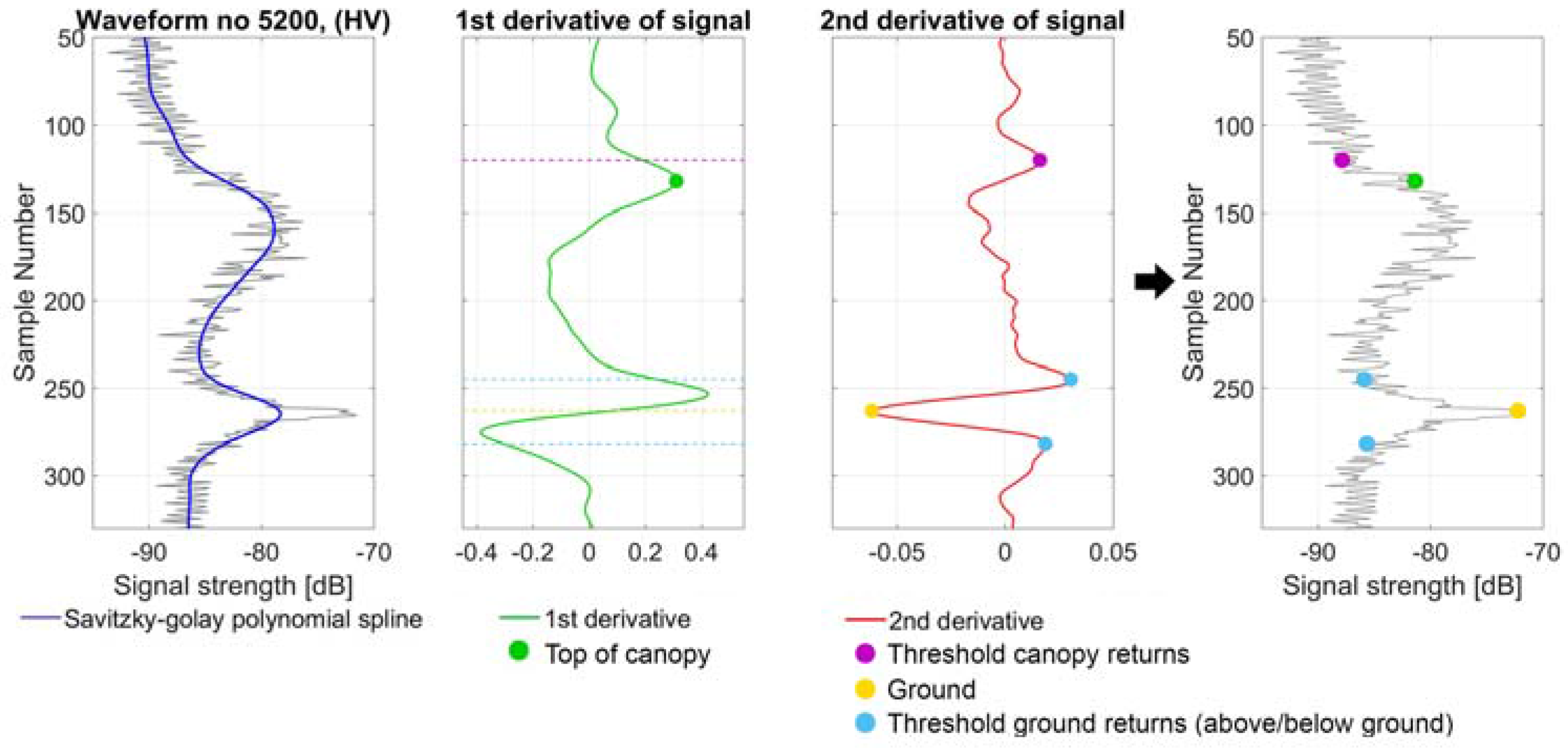
2.4.1. Detection of Ku-Band Ground and Canopy Profiles
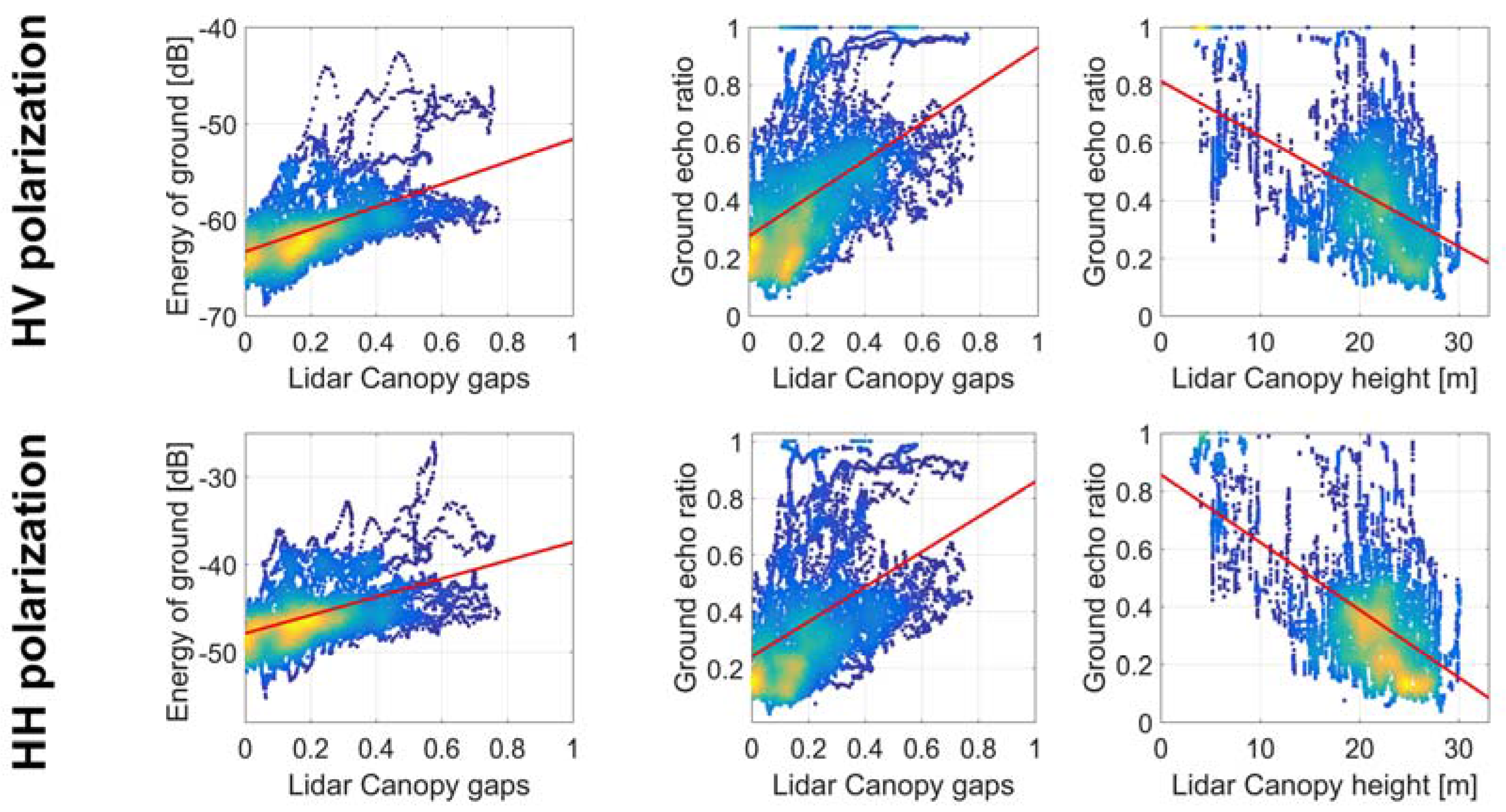
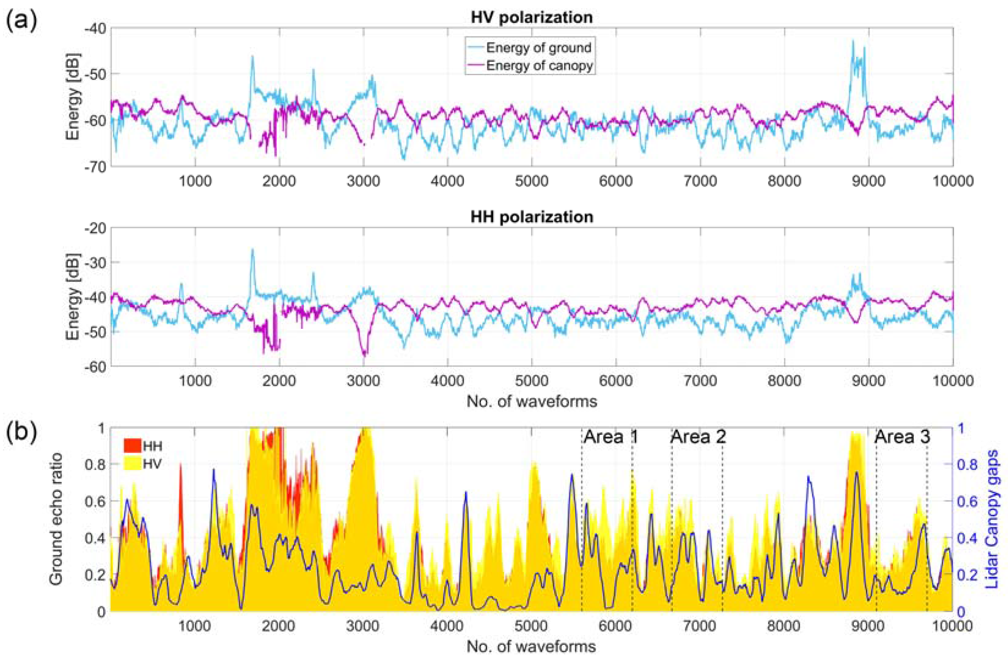
2.4.2. Analysis of the Energy of Ground, Canopy, and Ground Echo Ratio in Comparison with Lidar
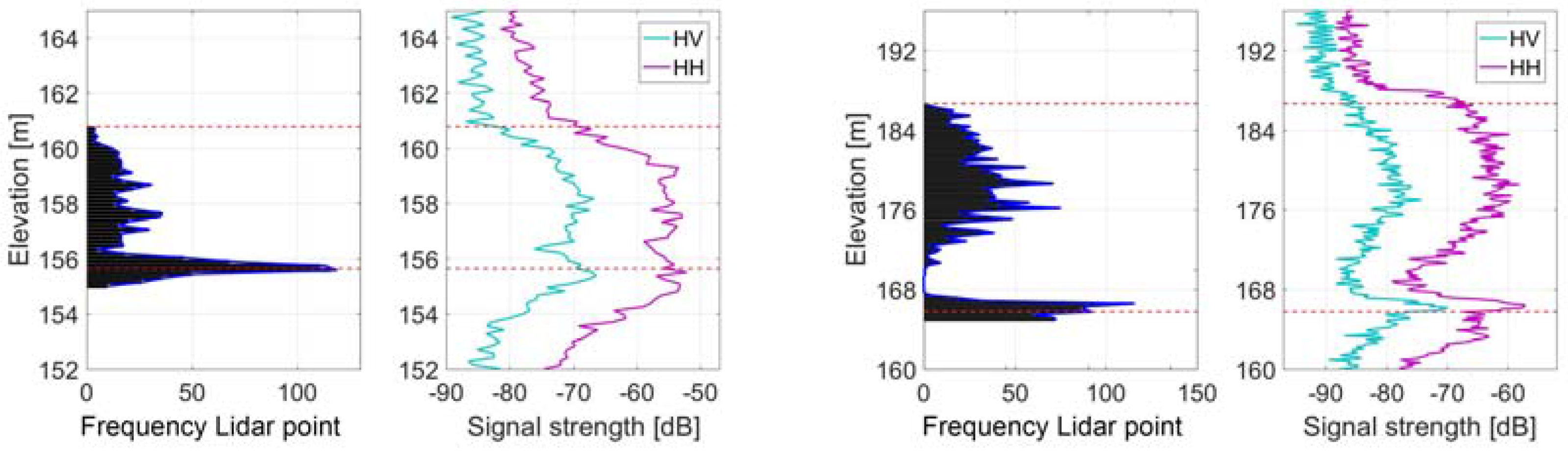
2.4.3. Validation of Signal Processing Method: Comparison of Waveform Features with Canopy and Terrain Elevation
3. Results
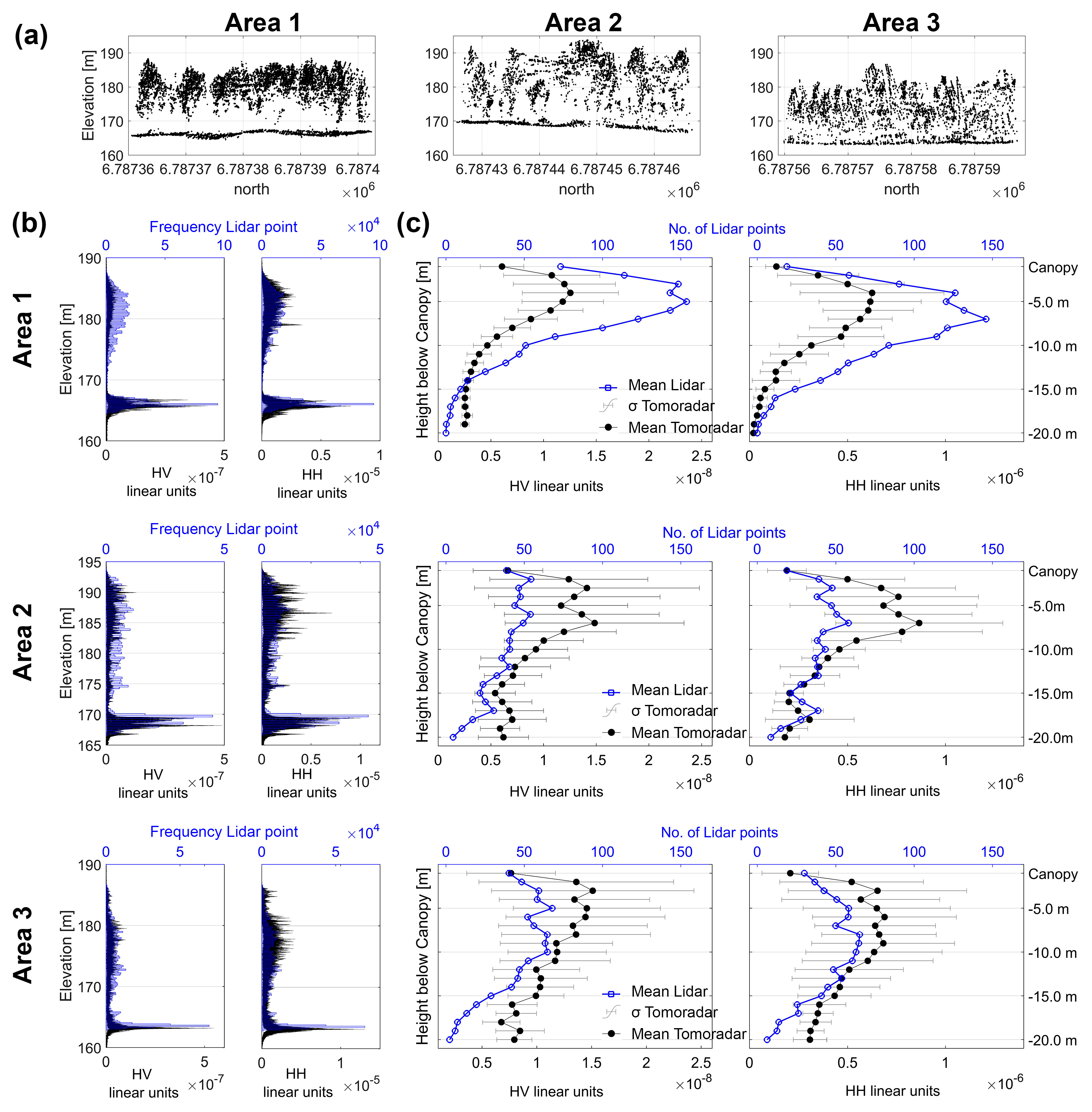
3.1. Quantitative Analyses of the Ku-Band Backscatter Signal Penetration
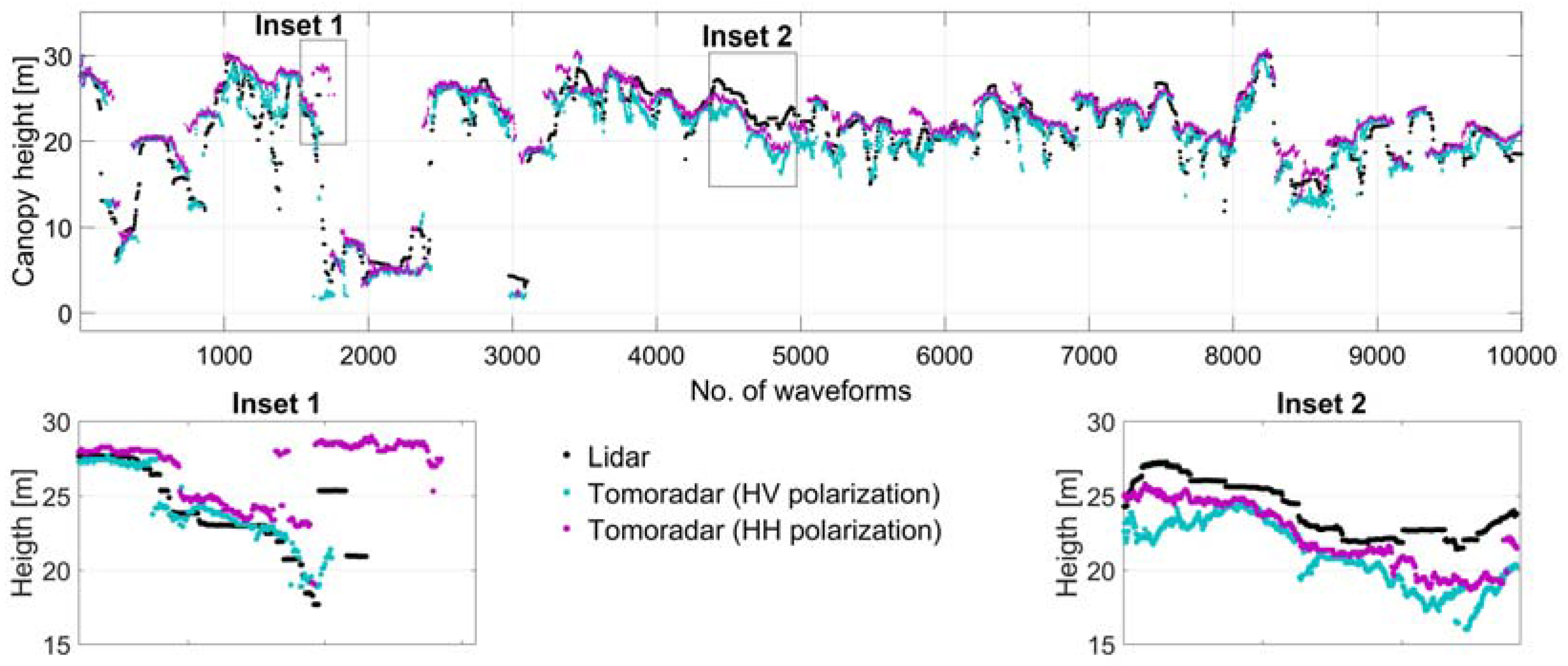
3.2. Estimation of Tomoradar Ground and Canopy Elevation Accuracy
4. Discussion
5. Conclusions
Acknowledgments
Author Contributions
Conflicts of Interest
References
- Ridder, R.M. Global Forest Resources Assessment 2010: Options and Recommendations for a Global Remote Sensing Survey of Forests. FAO Forestry Working Paper 141. 2007. Available online: http://www.fao.org/3/a-ai074e.pdf (accessed on 20 September 2017).
- Spies, T.A.; Spies, T.A. Forest structure: A key to the ecosystem. Northwest Sci. 1998, 72, 34–36. [Google Scholar]
- Hurtt, G.C.; Dubayah, R.; Drake, J.; Moorcroft, P.R.; Pacala, S.W.; Blair, J.B.; Fearon, M.G. Beyond potential vegetation: Combining lidar data and a height-structured model for carbon studies. Ecol. Appl. 2004, 14, 873–883. [Google Scholar] [CrossRef]
- Drake, J.B.; Dubayah, R.O.; Clark, D.B.; Knox, R.G.; Blair, J.B.; Hofton, M.A.; Chazdone, R.L.; Weishampelf, J.F.; Prince, S. Estimation of tropical forest structural characteristics using large-footprint lidar. Remote Sens. Environ. 2002, 79, 305–319. [Google Scholar] [CrossRef]
- Kellndorfer, J.; Walker, W.; Pierce, L.; Dobson, C.; Fites, J.A.; Hunsaker, C.; Clutter, M. Vegetation height estimation from shuttle radar topography mission and national elevation datasets. Remote Sens. Environ. 2004, 93, 339–358. [Google Scholar] [CrossRef]
- Andersen, H.E.; Reutebuch, S.E.; McGaughey, R.J. Active remote sensing. In Computer Applications in Sustainable Forest Management; Springer: Dordrecht, The Netherlands, 2006; pp. 43–66. [Google Scholar]
- Devaney, J.; Barrett, B.; Barrett, F.; Redmond, J.; O’Halloran, J. Forest Cover Estimation in Ireland Using Radar Remote Sensing: A Comparative Analysis of Forest Cover Assessment Methodologies. PLoS ONE 2015, 10, e0133583. [Google Scholar] [CrossRef] [PubMed]
- Perko, R.; Raggam, H.; Deutscher, J.; Gutjahr, K.; Schardt, M. Forest assessment using high resolution SAR data in X-band. Remote Sens. 2011, 3, 792–815. [Google Scholar] [CrossRef]
- Balzter, H.; Rowland, C.S.; Saich, P. Forest canopy height and carbon estimation at Monks Wood National Nature Reserve, UK, using dual-wavelength SAR interferometry. Remote Sens. Environ. 2007, 108, 224–239. [Google Scholar] [CrossRef]
- Soja, M.J.; Persson, H.; Ulander, L.M. Estimation of forest height and canopy density from a single InSAR correlation coefficient. IEEE Geosci. Remote Sens. Lett. 2015, 12, 646–650. [Google Scholar] [CrossRef]
- Solberg, S.; Astrup, R.; Bollandsås, O.M.; Næsset, E.; Weydahl, D.J. Deriving forest monitoring variables from X-band InSAR SRTM height. Can. J. Remote Sens. 2010, 36, 68–79. [Google Scholar] [CrossRef]
- Karjalainen, M.; Kankare, V.; Vastaranta, M.; Holopainen, M.; Hyyppä, J. Prediction of plot-level forest variables using TerraSAR-X stereo SAR data. Remote Sens. Environ. 2012, 117, 338–347. [Google Scholar] [CrossRef]
- Schmitt, M.; Brück, A.; Schönberger, J.; Stilla, U. Potential of airborne single-pass millimeterwave InSAR data for individual tree recognition. In Proceedings of the 33rd Wissenschaftlich-Technische Jahrestagung der DGPF, Freiburg, Germany, 27 February–1 March 2013; pp. 427–436. [Google Scholar]
- Tebaldini, S.; Ferro-Famil, L. High resolution three-dimensional imaging of a snowpack from ground-based SAR data acquired at X and Ku band. In Proceedings of the 2013 IEEE International Geoscience and Remote Sensing Symposium (IGARSS), Melbourne, Australia, 21–26 July 2013; pp. 77–80. [Google Scholar]
- King, J.; Kelly, R.; Kasurak, A.; Duguay, C.; Gunn, G.; Rutter, N.; Watts, T.; Derksen, C. Spatio-temporal influence of tundra snow properties on Ku-band (17.2 GHz) backscatter. J. Glaciol. 2015, 61, 226. [Google Scholar] [CrossRef]
- Rott, H.; Cline, D.; Duguay, C.; Essery, R.; Haas, C.; Macelloni, G.; Yueh, S. CoReH2O-A Ku-and X-band SAR mission for snow and ice monitoring. In Proceedings of the 7th European Conference on Synthetic Aperture Radar (EUSAR), Friedrichshafen, Germany, 2–5 June 2008; pp. 1–4. [Google Scholar]
- Hyyppä, J.; Hallikainen, M. A helicopter-borne 8-channel ranging scatterometer for remote sensing, Part II: Forest Inventory. IEEE Trans. Geosci. Remote Sens. 1993, 31, 170–179. [Google Scholar] [CrossRef]
- Morrison, K.; Bennett, J.; Solberg, S. Ground-based C-band tomographic profiling of a conifer forest stand. Int. J. Remote Sens. 2013, 34, 7838–7853. [Google Scholar] [CrossRef]
- Chen, Y.; Hakala, T.; Karjalainen, M.; Feng, Z.; Tang, J.; Litkey, P.; Hyyppä, J. UAV-Borne Profiling Radar for Forest Research. Remote Sens. 2017, 9, 58. [Google Scholar] [CrossRef]
- Feng, Z.; Chen, Y.; Hakala, T.; Hyyppä, J. Range calibration of airborne profiling radar used in forest inventory. In Proceedings of the 2016 IEEE International Geoscience and Remote Sensing Symposium (IGARSS), Beijing, China, 10–15 July 2016; pp. 6672–6675. [Google Scholar]
- Pfeifer, N.; Mandlburger, G.; Otepka, J.; Karel, W. OPALS—A framework for Airborne Laser Scanning data analysis. Environ. Urban Syst. 2014, 45, 125–136. [Google Scholar] [CrossRef]
- Savitzky, A.; Golay, M.J. Smoothing and differentiation of data by simplified least squares procedures. Anal. Chem. 1964, 36, 1627–1639. [Google Scholar] [CrossRef]
- Banskota, A.; Wynne, R.H.; Johnson, P.; Emessiene, B. Synergistic use of very high-frequency radar and discrete-return lidar for estimating biomass in temperate hardwood and mixed forests. Ann. For. Sci. 2011, 68, 347–356. [Google Scholar] [CrossRef]


| Parameters | |
|---|---|
| Modulation frequency | 163 Hz |
| Output frequency | 14 GHz (2.1 cm) |
| Range resolution (m) | 0.15 |
| Along-track sampling interval (m) | 0.06 |
| Spatial resolution | two-way antenna beamwidth < 6° |
| Transmit receive polarizations | HV/HH |
| Weight | Less than 5 kg |
| Data rate | 2.5 Mbits/s |
| Energy Entire Profile | Energy of Ground Selected Area (~36 m Profile) | Energy of Canopy Selected Area (~36 m Profile) | ||||||||||||||
|---|---|---|---|---|---|---|---|---|---|---|---|---|---|---|---|---|
| Polar. | Ground | Canopy | Area 1 | Area 2 | Area 3 | Area 1 | Area 2 | Area 3 | ||||||||
| Mean | σ | Mean | σ | Mean | σ | Mean | σ | Mean | σ | Mean | σ | Mean | σ | Mean | σ | |
| HV | −60.7 | 3.5 | −59.2 | 1.8 | −61.2 | 1.3 | −61.8 | 2.1 | −61.7 | 1.6 | −61.0 | 0.7 | −59.0 | 1.0 | −58.7 | 1.0 |
| HH | −45.5 | 3.5 | −43.2 | 2.5 | −46.9 | 1.0 | −47.1 | 1.8 | −46.2 | 1.4 | −44.3 | 1.0 | −42.2 | 1.1 | −42.1 | 1.1 |
| Ground Echo Ratio Entire Profile | Ground Echo Ratio Selected Area (~36 m Profile) | |||||||
|---|---|---|---|---|---|---|---|---|
| Polarized Channel | Mean | σ | Area 1 | Area 2 | Area 3 | |||
| Mean | σ | Mean | σ | Mean | σ | |||
| HV | 0.42 | 0.22 | 0.49 | 0.09 | 0.36 | 0.14 | 0.35 | 0.12 |
| HH | 0.38 | 0.23 | 0.36 | 0.08 | 0.26 | 0.11 | 0.28 | 0.11 |
| Data | Elevation Difference [m] | |||||||||
|---|---|---|---|---|---|---|---|---|---|---|
| Ground | Canopy | |||||||||
| Mean | σ | Median | RMSE | R2 | Mean | σ | Median | RMSE | R2 | |
| Tomoradar | ||||||||||
| HH-HV | −0.173 | 0.284 | −0.140 | 0.333 | 0.997 | 1.544 | 2.910 | 0.842 | 3.294 | 0.849 |
| Tomoradar-Lidar | ||||||||||
| HV-Velodyne | −0.033 | 0.440 | −0.112 | 0.441 | 0.993 | −0.584 | 2.422 | −0.586 | 2.492 | 0.930 |
| HH-Velodyne | −0.207 | 0.491 | −0.281 | 0.533 | 0.991 | 1.354 | 3.430 | 0.334 | 3.687 | 0.858 |
| HV-Riegl | −0.167 | 0.339 | 0.159 | 0.378 | 0.996 | — | — | — | — | — |
| HH-Riegl | −0.006 | 0.403 | −0.003 | 0.403 | 0.994 | — | — | — | — | — |
| Riegl-Velodyne | ||||||||||
| Velodyne-Riegl | 0.201 | 0.341 | 0.282 | 0.395 | 0.996 | — | — | — | — | — |
© 2017 by the authors. Licensee MDPI, Basel, Switzerland. This article is an open access article distributed under the terms and conditions of the Creative Commons Attribution (CC BY) license (http://creativecommons.org/licenses/by/4.0/).
Share and Cite
Piermattei, L.; Hollaus, M.; Milenković, M.; Pfeifer, N.; Quast, R.; Chen, Y.; Hakala, T.; Karjalainen, M.; Hyyppä, J.; Wagner, W. An Analysis of Ku-Band Profiling Radar Observations of Boreal Forest. Remote Sens. 2017, 9, 1252. https://doi.org/10.3390/rs9121252
Piermattei L, Hollaus M, Milenković M, Pfeifer N, Quast R, Chen Y, Hakala T, Karjalainen M, Hyyppä J, Wagner W. An Analysis of Ku-Band Profiling Radar Observations of Boreal Forest. Remote Sensing. 2017; 9(12):1252. https://doi.org/10.3390/rs9121252
Chicago/Turabian StylePiermattei, Livia, Markus Hollaus, Milutin Milenković, Norbert Pfeifer, Raphael Quast, Yuwei Chen, Teemu Hakala, Mika Karjalainen, Juha Hyyppä, and Wolfgang Wagner. 2017. "An Analysis of Ku-Band Profiling Radar Observations of Boreal Forest" Remote Sensing 9, no. 12: 1252. https://doi.org/10.3390/rs9121252