Annual Seasonality Extraction Using the Cubic Spline Function and Decadal Trend in Temporal Daytime MODIS LST Data


1
Department of Mathematics and Computer Science, Faculty of Science and Technology, Prince of Songkla University, Pattani Campus, Chang Wat Pattani 94000, Thailand
2
Faculty of Technology and Environment, Prince of Songkla University, Phuket Campus, Chang Wat Phuket 83120, Thailand
3
Climate Change Cluster, University of Technology Sydney, City Campus, Ultimo, NSW 2007, Australia
*
Author to whom correspondence should be addressed.
Remote Sens. 2017, 9(12), 1254; https://doi.org/10.3390/rs9121254
Submission received: 27 October 2017
/
Revised: 25 November 2017
/
Accepted: 29 November 2017
/
Published: 2 December 2017
(This article belongs to the Special Issue Remote Sensing for Land Surface Temperature (LST) Estimation, Generation, and Analysis)
Abstract
:Examining climate-related satellite data that strongly relate to seasonal phenomena requires appropriate methods for detecting the seasonality to accommodate different temporal resolutions, high signal variability and consecutive missing values in the data series. Detection of satellite-based Land Surface Temperature (LST) seasonality is essential and challenging due to missing data and noise in time series data, particularly in tropical regions with heavy cloud cover and rainy seasons. We used a semi-parametric approach, involving the cubic spline function with the annual periodic boundary condition and weighted least square (WLS) regression, to extract annual LST seasonal pattern without attempting to estimate the missing values. The time series from daytime Aqua eight-day MODIS LST located on Phuket Island, southern Thailand, was selected for seasonal extraction modelling across three different land cover types. The spline-based technique with appropriate number and placement of knots produces an acceptable seasonal pattern of surface temperature time series that reflects the actual local season and weather. Finally, the approach was applied to the morning and afternoon MODIS LST datasets (MOD11A2 and MYD11A2) to demonstrate its application on seasonally-adjusted long-term LST time series. The surface temperature trend in both space and time was examined to reveal the overall 10-year period trend of LST in the study area. The result of decadal trend analysis shows that various Land Use and Land Cover (LULC) types have increasing, but variable surface temperature trends.
1. Introduction
Satellite-based climate-related data, such as Land Surface Temperature (LST), play a critical role in monitoring climatological processes, land surface energy interactions and water balance at regional to global scales [1,2,3,4], as well as climate change impacts. LST is the skin temperature of the land surface measured at the interface between surface materials (top of plant canopy, water, soil, ice or snow surface) and the atmosphere [5]. Some of the most advanced and widely-used LST products are those from the Moderate Resolution Imaging Spectroradiometer (MODIS) on-board the NASA Earth Observation System (EOS) Terra and Aqua satellites, launched in 1999 and 2002, respectively. Both space-borne sensors detect and measure the Earth’s surface temperature four times per day, at 10:30/22:30 (Terra) and 13:30/1:30 (Aqua) local overpass-times. With a high temporal frequency of data observations, MODIS provides daily, eight-day and monthly LST data time series at two spatial resolutions (1 km and 0.05 deg. Climate model grids, CMG) [6].
The MODIS LST time series data have been used in many applications. Long-term LST data are studied to understand their dynamics and influencing factors. Stoppiana et al. [5] used ten years of both day and nighttime MOD11A2 products over Southern Italy to quantify the influence of topography, solar radiation and land cover on land surface temperature seasonality. Moreover, Frey and Kuenzer [7,8] studied the impact of Land Use and Land Cover (LULC) changes on long-term surface thermal properties in the Mekong Basin using MODIS LST data. In the MODIS LST product used in these studies, cloud gaps will typically appear when the data are masked for cloudy pixels. Some Urban Heat Island effect (UHI) studies have used MODIS LST time series data to investigate seasonal and long-term thermal effects of urbanization on the land surface and atmosphere conditions [9,10]. Yao et al. [11] used 15 years of MODIS LST to examine the temporal trends of surface urban heat islands (SUHIs) in 31 mega cities in China. Nevertheless, imputed values for all missing data is a prerequisite when using filter-based time series analysis methods that use a set of fixed filters (moving averages) to decompose the time series and detect the seasonal components. Many space-time interoperation techniques for missing MODIS LST [12,13,14,15,16] have been developed to reconstruct the surface temperature maps using spatially neighbouring cloud-free pixels to estimate the LST of cloudy pixels [17] and fill the temporal gaps using high temporal time series. These techniques require rather more complicated mathematical and statistical models, as well as a sufficient range of temporal data. However, some of them still fail to fully achieve time series reconstruction. Many long-term MODIS LST studies tend to neglect the gap issue and minimize the effect of missing values by averaging values per period (or land cover type or region) and normalizing values (e.g., temperature anomalies) across different years, which also take seasonality into account. Similar to other time domain data, LST time series consist of seasonal, trend and residual (or noise) components. Season usually has a direct influence on the long-term LST that creates fluctuation and variation in observed surface temperature values. This seasonal effect needs to be considered and managed adequately before future trend analysis. Previous long-term LST trend studies minimize seasonal variation by focusing on specific periods within a year (e.g., growing season) and different times (e.g., day/night time) instead of explicitly accounting for seasonality. One of the most commonly-used standard techniques is the averaging approach. It can diminish seasonal effects and simply reveal the trend of the data. However, it also reduces the number of observations and, in many cases, has insufficient data for inferential statistical analysis of trends.
Clouds directly generate gaps in MODIS LST time series, but other phenomena also contaminate the measured signal, including atmospheric perturbations and variable illumination and viewing geometry, as well as atmospheric correction processes [18] that cause noise and errors in the retrieval of LST. Noise and missing value patterns, especially in the tropical regions that have so much cloud cover and rainy seasons, cause uncertain values and long gaps in LST time series. It is difficult and inappropriate, in many circumstances, to estimate consecutive missing values in LST time series because the surface temperature within a given time span varies so much due to many reasons such as surface topography, altitude, land cover and climatic conditions. Moreover, it often requires a sizable amount of historical data and complicated methods to acceptably interpolate consecutive missing values in such LST time series data. With the lack of available existing methods of seasonal extraction suitable for time series with consecutive missing values, it is essential and yet challenging to detect seasonality in MODIS LST time series due to serial gaps and noises. Thus, a straightforward method is needed for detecting seasonality in the analysis of long-term LST data.
In this work, we propose an alternative semi-parametric method for extracting annual seasonality in MODIS LST data that have high variability and many successive gaps without any interpolation attempt for estimating missing values. The aim of this work is to extract the seasonal LST pattern using cubic spline functions as an uncomplicated non-parametric model and Weighted Least Square (WLS) regression (a parametric model). The approach involves (1) finding an appropriate curve fitted to the data using statistical goodness of fit as the optimality criterion and (2) obtaining an estimated curve that does not display too much rapid fluctuation by selecting the right number and placements of the spline function components. In this study, we are aware of making a necessary compromise between two curve estimations aspects, acceptable fit to data and the smoothness and continuity of the fitted curve. Lastly, we apply the method and analyse trends and seasonality over the island of Phuket, Thailand, a tropical island study area with forests and complex land use/cover patterns.
2. Materials and Methods
2.1. Study Area
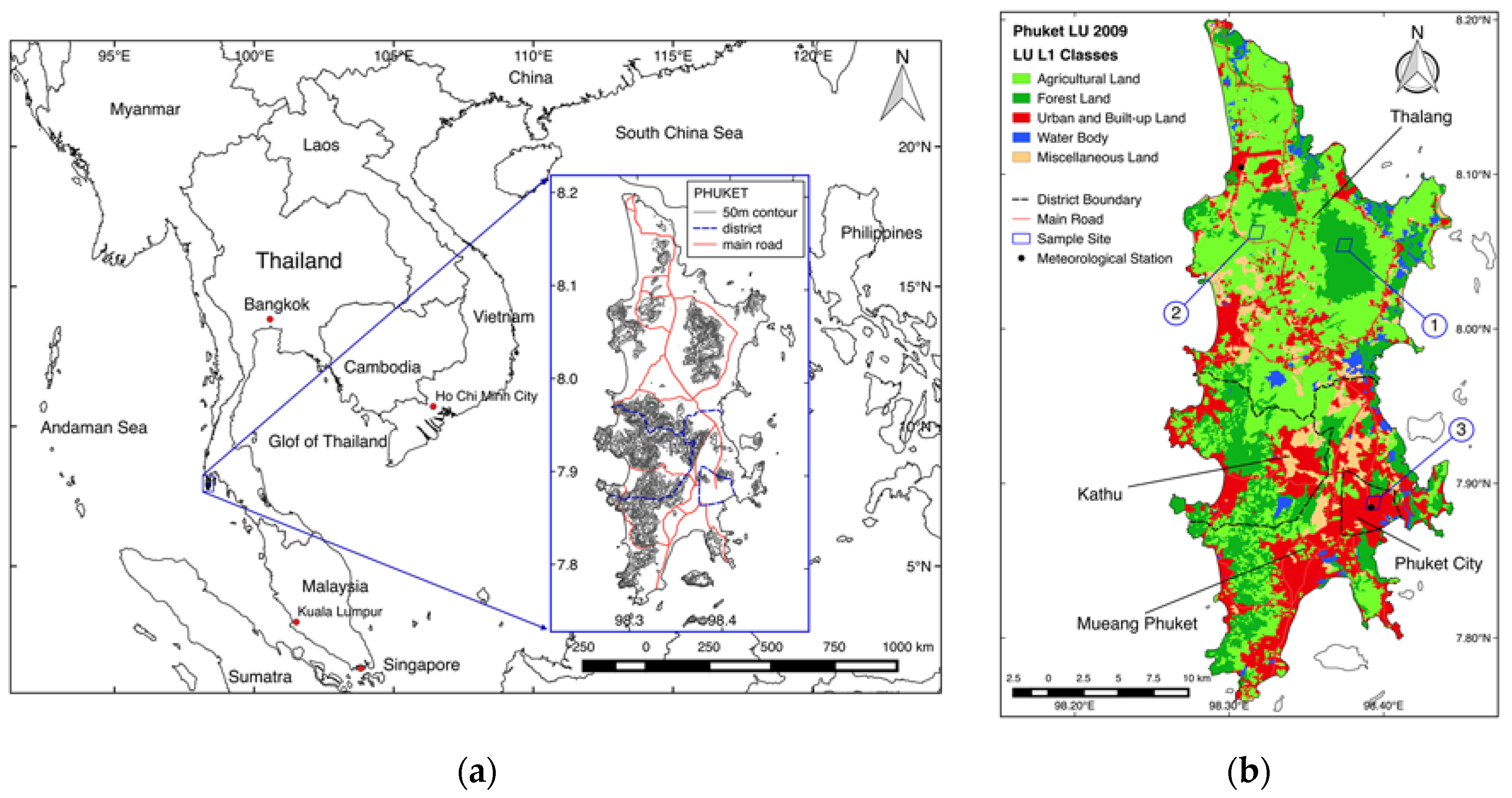
The study area is Phuket Island (see Figure 1). It has a tropical monsoon weather designation using the Köppen climate classification [19]. Its climate is typically divided into two distinct seasons, dry and rainy, with transitional periods in between. The dry season begins in November and usually lasts until March, which is influenced by the northeast monsoon that brings cold and dry air from the Asian continent. The rainy season starts in April and lasts until October. The strong wind of the southwest monsoon draws warm moisture from the India Ocean, resulting in plenty of rain. The average rainfall in Phuket is around 200–400 mm per month during the wet and humid period. Phuket Island is divided into three administrative districts and one local administration. The details of district area and its land cover are described in Table 1. The land use/cover distribution is illustrated in the map of the year 2009 LULC classification (Figure 1b). There are three major land cover types found in the study area are Forest (F), Agricultural land (A) and Urban and built-up land (U), according to the Level-1 LULC types classified by the Land Development Department (LDD), Ministry of Agriculture and Cooperatives of Thailand. The inland Water bodies (W) are mostly dams, canals, old mine pits and aquaculture farms that comprise 1.5% of the entire island area. The abandoned open ground mines, which eventually turn into scrub, open woodland and grassland, comprise the primary land use type of Miscellaneous land (M) that cover around 7.1% of the study area. Figure 1b also shows the locations of three samples of 1-km MODIS LST pixels with 1:30 p.m. overpass-time MODIS LST time series that were extracted from and subsequently were used to model annual seasonality. The details of the sample sites location and their LULC types are described in Table 2.
2.2. Data
2.2.1. MODIS LST
The Collection-6 (C6) daytime MODIS/Terra and MODIS/Aqua land surface temperature and emissivity eight-day composite L3 global 1-km sinusoidal grid products (MOD11A2 and MYD11A2) downloaded from the Global Subsets Tool [20] were used in this study. The C6 MODIS LST/emissivity products have a much better quality than the qualities of the C4.1 LST product (produced by the version 4 algorithm from C5 input data) and C5 products (generated by the version 5 algorithm from C5 input data) because they provide more stable results. Detailed validation of the new version of MODIS LST products is given in the most recently published paper [18,21]. As one of the aims of this study was to demonstrate how to apply the cubic spline function for detecting seasonal patterns in satellite-based temperature data, three samples of daytime temperature time series were extracted from a MYD11A2 product (LST_Day_1km). Moreover, its product quality control layers (QC_day), which provide information on the accuracy of the retrievals, were also used. Each time series consists of a total of 690 observations (4 July 2002–26 June 2017), which is precisely 15 years of data observation. Moreover, daytime LST data from both MODIS sensors on Terra and Aqua satellites were also used to apply the proposed pixel-based seasonal extracting method and further decadal trend investigation.
2.2.2. Meteorological Data
The 15-year historical weather data acquired from the National Climatic Data Center (NCDC) under public access provided by NOAA’s National Center of Environmental Information (NCEI). The data collected from two meteorological stations in the study area were used to compare the trend of seasonality produced from the proposed seasonality extraction method with the local climate. The daily average surface air temperatures, including maximum and minimum temperature reported during the day from the year 2002–2016, reduced the effect of variation by averaging into monthly data. However, only climatic data from the meteorological station located in Phuket downtown were used in comparison with the seasonality of LST extracted from Study Site 3, which is an urban and built-up land cover site, because the region of the study site covers the location of the meteorological station (see Figure 1b).
2.3. Methods
2.3.1. Cubic Spline Function
A k-th order spline model is a well-known, numeric curve fitting function with derivatives that users can define as necessary for its applications [22]. Not only the degree of the spline function, but other parameters such as a number of polynomial pieces connecting points (known as knots), the position of the knots and the free coefficients of the spline function are the user’s choice [23]. The most commonly-used spline is a cubic spline, of order 3. A cubic spline function is a piecewise cubic polynomial with continuous second derivatives and is smoothest among all functions in the sense that it has a minimal integrated squared second derivative. Moreover, it is easily fitted using linear least squares regression [24]. The cubic spline function is widely used for smoothing data in various fields of study such as interactive computer graphics [24,25], real-time digital signal processing [26,27,28] and satellite-based time series data [29,30,31,32,33,34]. The main advantages of the spline fit are that the first and second derivatives are continuous [24], including its simple calculation, good stability, high precision and smoothness [30]. The gradients derived from cubic spline functions are smoothly joined parabolas, not the abruptly joined straight line segments characteristic of parabolic spline smoothing [35].
As MODIS LST data are collected over time, they fluctuate over the season. The seasonal pattern is assumed to be the same for every year, and the change in other parameters such as the land cover change that has a direct or indirect effect on the LST data is consistently increasing or decreasing. A sudden natural disaster, for instance a forest fire or landslide or tsunami that could cause the instantaneous change of data behaviour, is excluded in this model consideration. Ideally, the model should provide continuous seasonal patterns for each day of the year within a year. These considerations suggest that the most appropriate model is a cubic spline with specific boundary conditions that ensure smooth periodicity. The model and all of the parameters are illustrated in Figure 2. The formula for a cubic spline function is:
Where denotes time, are specified knots and is for and 0 otherwise.
In this case, we need a special annual periodic boundary condition that requires the quadratic and cubic coefficients of the spline function to be 0 for and , where and are the location of the first knot and the last knot, respectively. The functions (between and ) and (between and ) are linear functions with the same slope. Thus, the following two equations must be satisfied:
To ensure a smooth and continuous curve at the start and the endpoint, the slopes at and need to be imposed, and they need to be equal. However, the values at the end and the start points are not necessarily matched in order to allow the trend to appear in the function. When considering at , the function beyond is linear as the function before . Therefore, in all derivatives of the cubic polynomial (, where is the degree of the spline function).
Thus, , which makes and consequently, . Incorporating two constraints (Equations (2) and (3)) into the equation above, therefore,
In this case, the cubic spline function with degree 3 needs free coefficients, where is the number of knots (each polynomial piece has coefficients, and the continuity conditions introduce bands per knot, leaving free coefficients), then the cubic spline function can be rewritten as:
where:
This cubic spline function was used in this study to capture the seasonal component in LST time series within the annual period. Note that this cubic spline function has a dissimilar boundary condition from the “periodic end condition” when the cubic spline function satisfies the following condition [25]: , , and for a natural cubic spline.
2.3.2. Knots Selection
Choosing the location and number of knots for smoothing the spline curve is a critical issue. However, there are current strategies for the optimal selection of those parameters based on procedures to add knots in intervals where the residuals show trends as indicated by autocorrelation or in intervals where the residuals are inadmissibly significant [23]. The number of knots corresponds to the number of linear segments. More knots would result in a smoother covariance surface, but would require more parameters to estimate. Locations of knots should correspond to the pattern of changes along the curve. Rapid changes require a larger number of knots in a given region, whereas small changes would need a sparser distribution of knots [36].
There are, practically, two distinctive philosophical approaches in choosing the optimal number and placement of knots. The first one is the subjective choice, for which one could place more knots where the data vary the most rapidly, and fewer knots where they are more stable. It is one of the advantages of using cubic spline that the data can be obtained at unequal intervals [37]. In contrast, there could be as few knots as possible to ensure that there are at least 4 or 5 points per interval for the cubic spline [22]. This restriction corresponds to the usual practice of keeping the number of parameters as small as possible since the flexibility of the spline function could over-fit. The second approach is the automatic method where the optimal knots are chosen directly by the data. This objective approach would be to use an iterative algorithm for the free knot spline [38] where the spline parameters are automatically estimated using uniform quartiles to find the knot positions and generalized cross-validation [39,40] to quantify the appropriate number of knots to be used. The basic idea of leave-one-out cross-validation is to omit some portion of data randomly and fit the model using the remaining data, then to use the fitted model to make predictions on the omitted data. Finally, the errors are computed (called predicted residuals). The step is repeated multiple times, and then, the Mean Square Error (MSE) is calculated from the predicted residuals (called cross-validated errors).
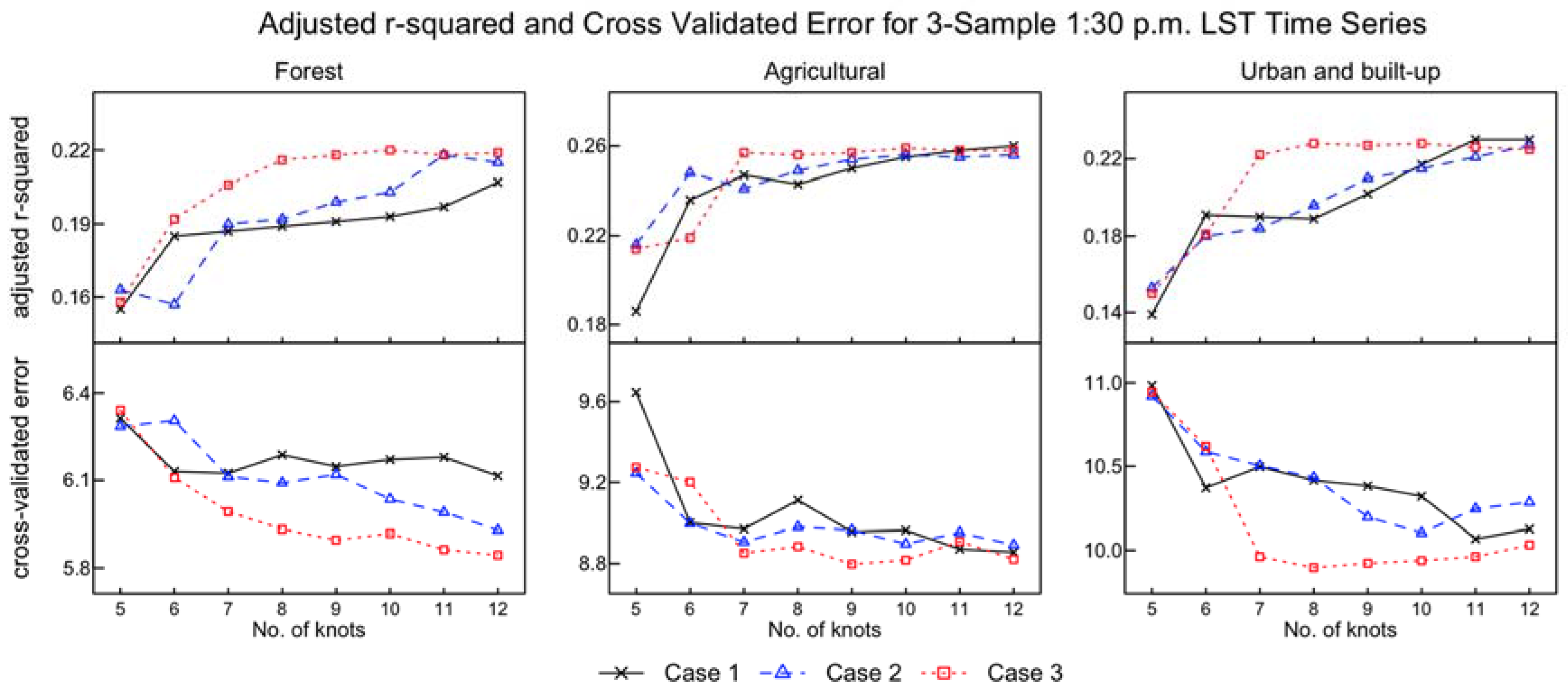
To select the optimal number and placement of knots to be used with LST data in this study, we compromised between goodness of fit and smoothness of the seasonal curve. Figure 3 shows the result of the adjusted r-squared and cross-validated error, respectively, when we varied the number of knots in different scenarios of their position. The criteria of three separate cases, which are subjected to the knots placement method, are (1) knots are placed at an equal interval (denoted by Case 1), (2) knots are placed at uniform quartiles (denoted by Case 2) and (3) knots are placed at a “best practice” locations (denoted by Case 3). The “best practice” knot locations are defined based on the actual behaviour of the LST data. LST data, especially in the tropical region, generally have high proportions of missing and highly variable data during the rainy season. We fix four knots at Julian Days 10, 115, 310 and 350 to avoid misplacing knots in the high variation and low distribution of data segmentation and to ensure that at least two knots are located near the beginning and the end of the annual range. Then, we allocate the rest between those four knots by equal intervals to cover the rapid change of the curve. It is important that the knots be located where the data are stable and not too far from the beginning and the end of the annual data series to ensure a continuous seasonal pattern between years.
2.3.3. LST Outlier Elimination
Since we fit the annual climatological profile using spline functions, all 15-year data series were re-ordered into Julian days. Extreme values can be detected for each group of data at each Julian day using the Interquartile Range (IQR). However, this outlier detection method may not adequately filter out the extreme values where there is less data density and the LST values separate from other values in a specific Julian day. The simple additional anomaly detection using the 3-sigma rule could be used if the entire time series were normally distributed. Any LST value that exceeds three standard deviations from the norm (±3σ) was thus marked as an outlier.
2.3.4. Weighted Least Squares Regression
Due to the negative effects on a number of phenomena that contaminate the measured LST signal, including clouds, atmospheric perturbations, variable illumination and viewing geometry [37], which tend to cause fluctuation in the LST values, weighted least squares regression can be applied to penalize negative errors instead of using an ordinary least squares regression. The method of Weighted Least Squares (WLS) regression can be utilized when the Ordinary Least Squares (OLS) assumption of the constant variation in the errors is violated and is less sensitive to large changes in small parts of the observations. The WLS method is adopted in this study as a way of dealing with heteroscedastic errors. WLS can be achieved by minimizing the weighted sum of squares,
where are weights inversely proportional to the variance of the residuals (i.e., ). This includes OLS as the special case where all the weights .
In this study, we set the rule as extreme LST values are given zero weight () and give a score range from 4–1 according to the quality control data [5,6]. We give a score of 4 when average LST error ≤ 1 K, a score of 3 for average LST error ≤ 2 K, a score of 2 for average LST error ≤ 3 K and a score of 1 for average LST error > 3 K.
3. Results
3.1. Placement and Number of Knots
From the optimal knots sensitivity testing result, as shown in Figure 3, the “best practice” approach for knots placement (Case 3) could enhance the periodic cubic spline model fitting, which gives high adjusted r-squared and low cross-validated error in all sample LST time series when the number of knots is larger. The Case 3 lines have constant values of the goodness of fit and error after using eight or nine knots in most of the sample data series. Increasing the number of knots gives no better fit to data and tends to have more errors when using more than 10 knots. Additional knots contribute to the roughness of a curve that appears in highly fluctuating LST data. Using eight knots as the “best practice” may be more appropriate in this case. We can achieve our aim to trade-off between suitable curve fitting and a smooth, good-looking curve. Moreover, this approach introduces fewer free coefficients in the cubic spline function, which ensures that data are not overfitted.
3.2. Annual Seasonal Patterns of LST Time Series
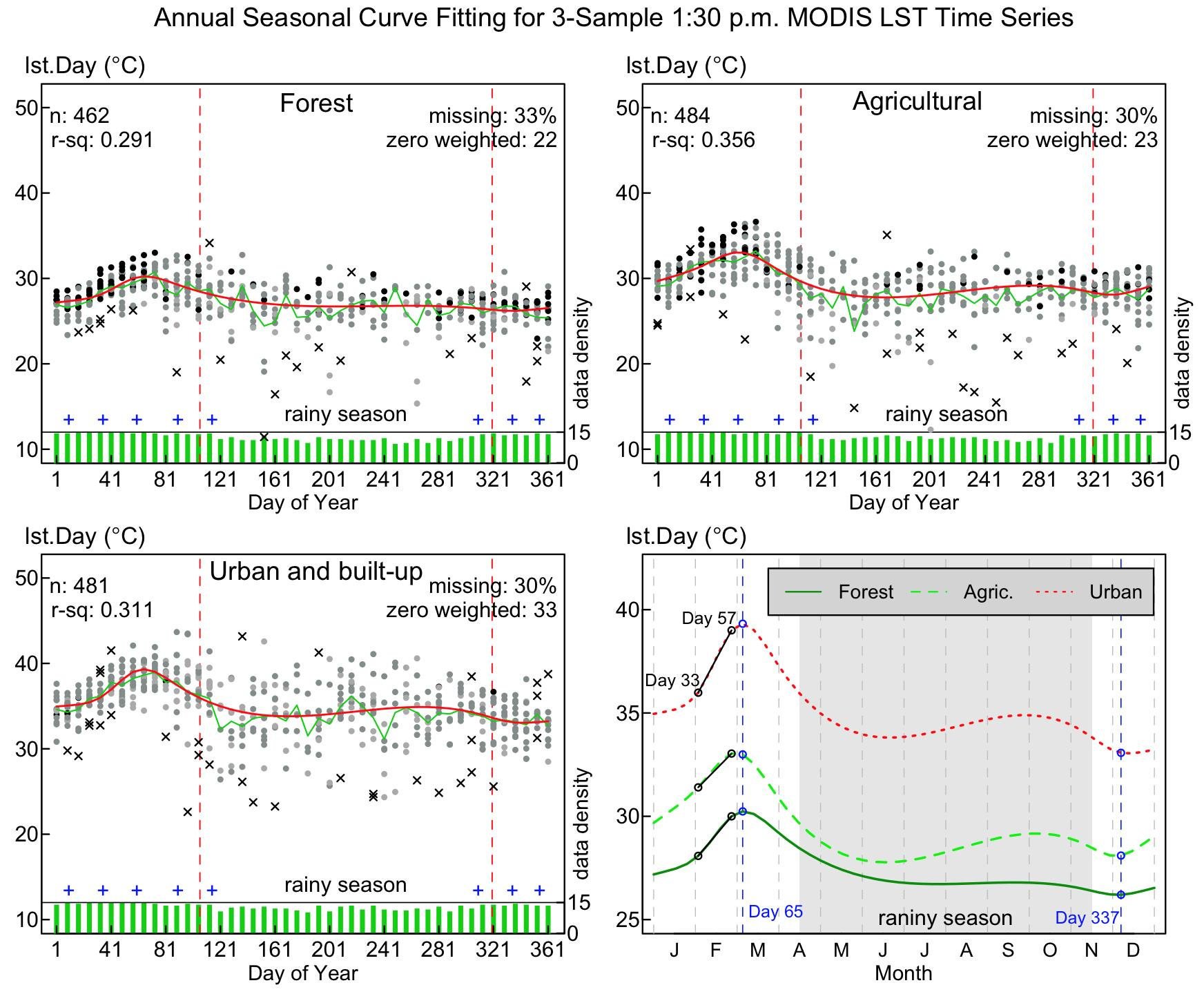
Figure 4 demonstrates how the cubic spline curve tracks the pattern of the LST data in the annual period when choosing eight knots at the “best practice” location. The estimated seasonal component was calculated after eliminating all extreme LST values and applying WLS regression using the weighted conditions as described in Section 3.3. The adjusted r-squared values display how well the proposed cubic spline function with optimal knots and their appropriate allocation fitted the data. Although they are not considered to be the best fit, we cannot accomplish a better fit to the data due to the high variability from different years in the LST data. This is typical behaviour for satellite-based temperature data, especially in the tropical climate region. The weighted regression that considers the outliers and the bias from data measurement error produces a curve more closely reflecting the actual trend of the data. The proposed cubic spline function with the unique boundary condition produces a smooth seasonal curve when compared to the eight-day and monthly average MODIS LST, as shown in Figure 5. Averaging data in a specific period is the traditional approach to overcome the missing value issue and variability in the data. When averaging data within a short period, there is high fluctuation in seasonality due to a high variation in LST data. The smoothness of seasonality could be achieved when a longer span of data was used in averaging. However, this means the number of data is significantly reduced, as well. Figure 5 also shows the trend of seasonality from the urban and built-up site along with the trend of monthly surface air temperature measured from the meteorological station at the study site that represents the local weather. Although the surface skin temperature (Tskin) and the surface air temperature (Tair) are different measures with regard to both their physical meaning and their magnitude (an absolute value of LST is usually higher than the surface air temperature), the two temperatures are complementary in their contribution of valuable information in climate study [41]. LST has been used for mapping and estimating surface air temperature in the different parts of the globe [42,43,44,45]. The seasonal curve resulting from the cubic spline function shows a similar pattern and trend to the local monthly average air temperature.
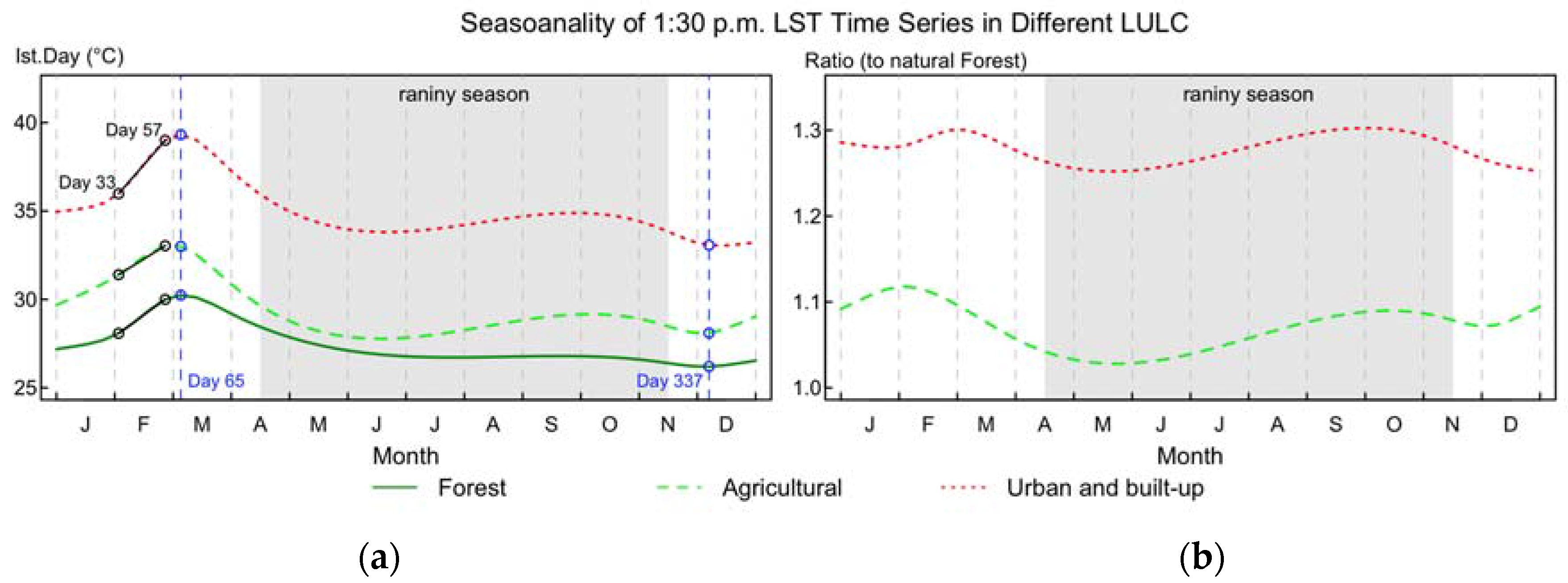
The surface temperature is constant during the wet season, despite the high variation and less intensity of data during this time. It keeps a steady level until early December, which is a month after the formal end of the rainy season. This delay of time could be because high moisture is still stored in the ground during the rainy season, as well as the variation of seasons in different years. The surface temperature starts rising around the middle of December and touches the highest point around late February to the middle of March. The surface temperature then begins to decrease when the first rain of the southwest monsoon comes around late March, often followed by more rainfall. However, the regular local rainy season usually starts in April, when the amount of rainfall and the number of the rainy days are substantial. Figure 6a shows the annual seasonality of sample LST data from forest, agriculture and urban land cover sites. The temperature of the urban surface is the warmest in all months, while the forest surface is the coolest. The rising rate (the slope from Julian Day 33–57 where the rising seasonality curve has maximum linearity during this period) of the urban impervious surface temperature during the drying out phase is approximately 0.126 °C/day. It is also higher than the rising temperature of the forest and agricultural area, which are approximately 0.079 and 0.068 °C/day, respectively. The difference between the maximum (at Julian Day 65) and minimum (at Julian Day 337) surface temperature during the dry season (ΔTdry) for the urban surface site is also higher than other locations. The ΔTdry of the urban site is around 6.03 °C, whereas the ΔTdry of the entire forest and agriculture land cover sites is around 4.03 and 4.89 °C, respectively. The urban and built-up land surface causes more variability of maximum and minimum surface temperature during the dry period. Figure 6b displays the ratio of surface temperature seasonality in urban and agricultural land cover area to the forest (Surban/Sforest and Sagric./Sforest). It highlights the impact of urbanization and agriculture land use on natural surface vegetation.
3.3. Application to Daytime MODIS LST Data
We applied the proposed seasonal extraction method to the morning and afternoon LST data from MOD11A2 and MYD11A2 products. The data observed in the daytime MOD11A2 data (10:30 a.m. overpass-time) starts from 5 March 2000, which is two years earlier than the daytime MYD11A2 data (1:30 p.m. overpass-time). However, for the simplicity of data processing and comparing the result, we decided to select data observation from 4 July 2002–26 June 2017, which are 690 observations in total (46 observations each year for precisely 15 years). There are 611 MODIS LST pixels within Phuket Island excluding one pixel situated over the Bangwad dam. The seasonal component was calculated in a series by series (pixel by pixel) procedure. There is no distinction of the seasonal pattern found in the daytime MODIS LST datasets since our study area is considered as local scale with the same local weather and seasonal effect throughout the area. Therefore, we selected eight knots and placed them as the “best practice” position, which gives the best goodness of fit in the optimal knots process for both 10:30 a.m. and 1:30 p.m. LST datasets, to all LST time series located over the Phuket Island.
Once the seasonality is identified, the seasonal effect can be eliminated from the data series. This process is called seasonal adjustment, or deseasonalizing. Since the seasonal component from the spline-based seasonal extraction process is the additive model [46], the seasonally-adjusted series was determined by subtracting the LST series from the seasonal component and then adding the differentiation of averaged seasonal component and averaged seasonal subtracted LST, which is denoted as:
where is the seasonal component and is the observation ordered in the data series. Then, the LST data had become a stationary time series. Subsequently, detecting the lag one autocorrelation in the seasonal stationary data using first-order autoregression model, written as AR(1) [47,48], is required. If the autocorrelation is found, then it can be eliminated using linear filtering [49]. This procedure is vital to time series data analysis to meet the assumption of random error terms (independent errors), especially when fitting the linear trend using the OLS regression model. Autocorrelation in data will cause standard errors of regression coefficients to underestimate the true standard error and produce narrow confidence intervals. We found that the maximum lag one autocorrelation in 10:30 a.m. and 1:30 p.m. LST data is 0.26 and 0.24, respectively. There is around 25% of the time series that requires being filtered using a linear filter (reverse subtraction) to remove the autocorrelation influence. Finally, the surface temperature trend of the sufficient number of LST observations was directly estimated using a linear regression model, and the p-value can be obtained to weight the strength of the evidence.
3.3.1. Spatial Distribution of Daytime LST Trends
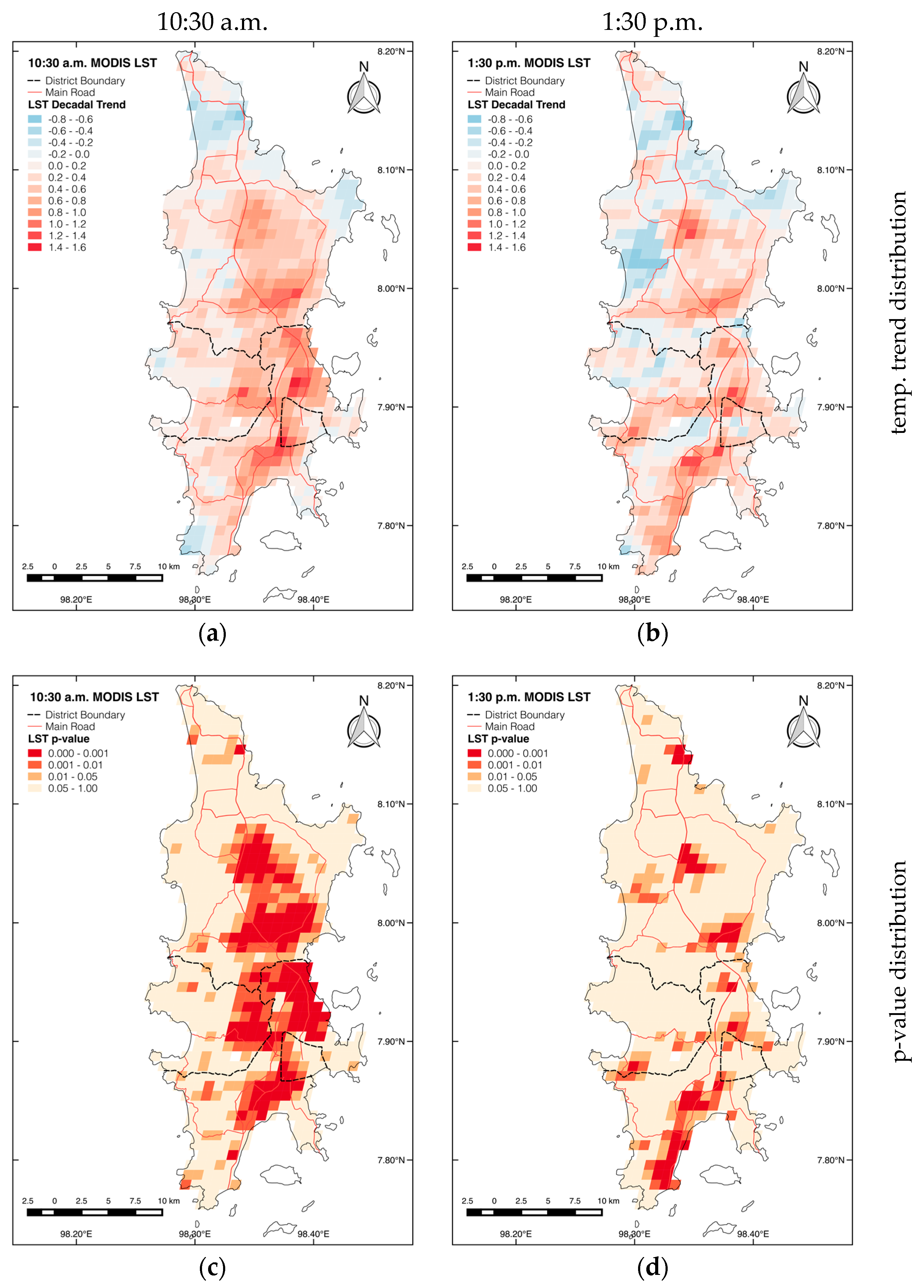
To observe the linear trend for each LST time series, the linear least squares estimation can be used to fit the data with any function of the form for . A method is a general approach that estimates α and β by minimizing the sum of squared deviations observed from expected responses. The linear model can be used over long ranges of data, but it is assumed to have poor extrapolation properties and sensitivity to outliers. When dividing the β parameter with the Δx in the LST time series, we can obtain the level of temperature change during the Δx period. Although we have data for 15 years and we can find the linear trend of LST over the 15-year time, a “decadal” trend of temperature change seems to be more appropriate and more widely used in the scientific community. The result of 10-year period LST trends can be depicted as thematic maps. Figure 7a,b displays the distribution of the trends of 10:30 a.m. and 1:30 p.m. MODIS LST time series, respectively. The p-value of linear trends for each LST series are demonstrated in Figure 7c,d. The diurnal LST displays a high positive surface temperature trend occurring along the main road surrounding Phuket City boundary. The areas that have warming surface temperatures higher than 1 °C per decade with high statistical significance (p-value < 0.01) appear mostly in the agriculture lands (~54% for 10:30 a.m. and ~76% for 1:30 p.m. LST data) and urban area (~20% for 10:30 a.m. and ~10% for 1:30 p.m. LST data).
3.3.2. Trend of Daytime LST in Different LULC Types
We further investigated the overall trend of daytime LST in all LULC types in the entire study area. To discover the overall LST trend for more extensive area, we used the Generalized Estimating Equations (GEEs) [50,51]. GEE is a general statistical approach to fit a marginal model for longitudinal/clustered data analysis [52]. The GEE method takes clustered correlations into account by means of keeping high correlations within the group and fewer correlations between the group. This statistical model is ideal for time series analysis of multiple series such as temporal LST from many locations that have a spatial correlation with other nearby locations. Figure 8 shows the overall trends of land surface temperature in various LULC types and areas of 10:30 a.m. and 1:30 p.m. MODIS LST datasets. The LST data have been grouped into five main LULC categories and four administrative regions. In each LULC group, there is the combination of uniform and mixed land cover types in a 1-km2 LST pixel area. In the study area, there are 0.24 and 0.12 °C increases in the surface temperature in a decade for the 10:30 a.m. and 1:30 p.m. datasets, respectively, and those uprising trends are statistically significant. All diurnal surface temperature trends are warmer in all various land cover types and areas. The rising surface temperature trend in the morning is higher than in the afternoon. The overall LST trends, both 10:30 a.m. and 1:30 p.m. overpass-time, in the miscellaneous land (total 39 time series) increase more than in other areas. The second warming trend is found in the urban area (total of 62 time series), followed by the forest (total of 92 time series) and the agricultural (total of 389 time series) land cover areas. However, the afternoon LST trend in a cultivated area is more significant than in the forest area. Moreover, LST trends in Phuket City and Mueang Phuket districts, which have an extreme density of asphalt streets and concrete buildings, are higher than Thalang and Kathu districts, which are mainly para-rubber plantations and upland evergreen rain forest, respectively.
4. Discussion
The daytime MYD11A2 subset of data over the study area contained a large percentage of high-quality data, which was greater than 67% of the total observations. There were 33% of missing observations from the selected forest site and 30% missing observations from the sample agricultural and urban sites, as shown in Figure 4. The primary cause of missing data is due to a cloud and other sensor-related artefacts resulting from sun-sensor geometries and aerosols. The LST retrieval in C6 daily MODIS LST product series (MOD11A1 and MYD11A1) is retrieved using the generalized split-window algorithm under clear-sky conditions (at a confidence ≥95% over land that has an altitude ≤2000 m or ≥66% over land that has an altitude >2000 m and at a confidence of ≥66% over lakes) [6,53]. During the C6 Level-3 data processing, the cloud-contamination LSTs are removed by using constraints on the temporal variations in clear-sky LSTs over a period of 32 days by the refinement implemented in Product Generation Executive code (PGE16) [26], and they are indicated as zero (as missing value) in the obtained C6 eight-day composite MODIS LST dataset; although the proportion of gaps produced by missing daily observations is reduced mainly because of the compositing over eight-day periods of the daily LST product. Moreover, LST values that pass the cloud filter could still be subjected to a degree of cloud contamination causing data quality issues. The information about the quality of measured LST data is flagged in the quality control (QC) for LST and emissivity data. From the sample time series, the problem of missing data, which is indicated by the green bar in Figure 4, occurs more during the wet period of the year. High variability of surface temperatures is also found during the wet season.
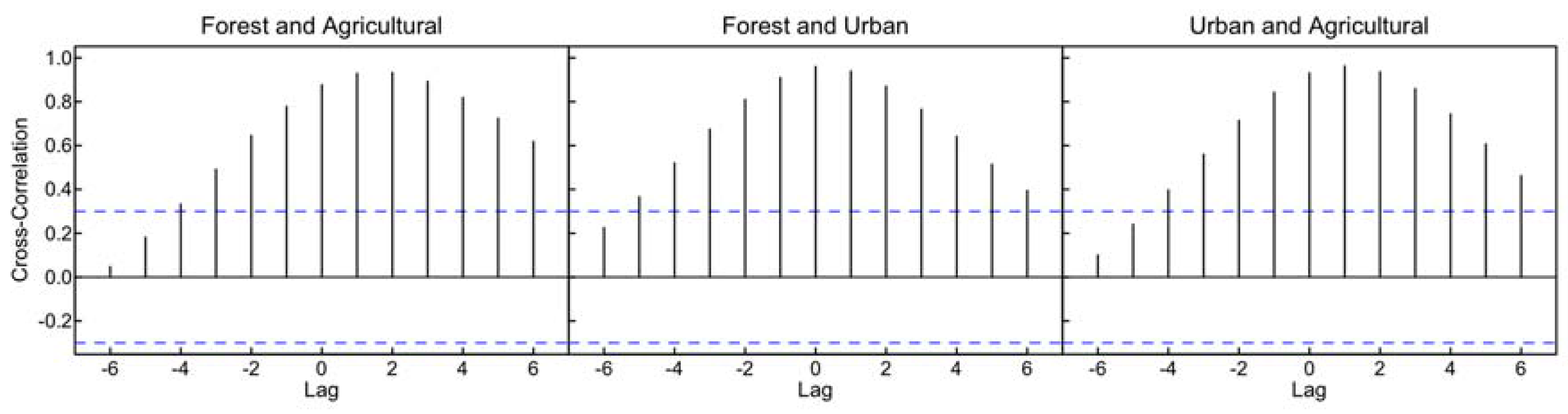
Despite the missing value issues and the fluctuation of LST values, the particular boundary restricted cubic spline function with optimal knots successfully achieved the extraction of annual LST seasonality. The pattern of seasonality from the three study sites was generally similar, except for the magnitude of seasonality, which varied for the different land cover types. The impervious surfaces such as asphalt road, concrete ground/building and manmade rooftop materials in the urban area absorb the Sun’s energy during the day more and faster than natural landscapes such as soil and vegetation. Thus, the overall magnitude of LST seasonality from the urban surface is the highest whereas that from the natural forest is the lowest. The cross-correlation coefficients, which are for comparing the temporal structure and mutual information of the signals, were between 0.877 and 0.960, and there were insignificant time shifts among the three seasonal profiles. Figure 9 displays the plot of the cross-correlation function that shows that the seasonalities from natural forest and urban sites have the most similarity. The graph of cross-correlation function indicates two identical series when the graphs on the positive and negative lag are symmetric. Table 3 also shows the normalized cross-correlation coefficients with time shift between the seasonality of the three different study sites. Both seasonal patterns from natural forest and agricultural sites highly correlate (0.933) with the time shift of two observation points (16 days). There is the highest correlation (0.963) of seasonality with the time shift of one observation point (eight days) from the urban and agricultural sites, whereas there is no time shift between seasonality from the forest and urban sites with cross-correlation at 0.960. Although the seasonal curve produced by the proposed cubic spline function is predominantly resulted from the optimal number of knots and their placement, if the same interval of knots is applied for the entire LST time series at such a local scale, it will extract similar seasonality of LST according to the local weather and season that persistently affect the surface temperature. In the case of extending the method over broader area coverage, such as at regional or global scales, the investigation of the different seasonal patterns may need to be conducted. The different optimal numbers of knots and their placements may need to be applied to the LST time series in the diverse regions.
One particular statistical method that delivers an excellent fit to data and produces a seasonal curve that reflects the real seasonality is the WLS regression, which had been applied to fit a cubic spline function to the data instead of using OLS regression. The main advantage of weighted regression is that it works well when successive false lows are rare so that local valleys occur separately [54,55]. However, it is not appropriate to use when several false lows occur in sequence because it results in false local peaks, which bias the estimated value downwards. This approach might not be suitable for daily data, and its applicability will depend on the frequency of cloud contamination and the strength of seasonality. In this study, we applied this robust weighted regression on LST data annually where each point of observation (46 observations for each year) contains a minimum of one value to a maximum of 15 values. Hence, the behaviour of the data may not cause any drawback of this model for this circumstance. Although there is a possibility that there are missing values at particular Julian days for the entire 15 years of LST observations, which could be found during the wet season, this occurrence is infrequent and does not consecutively happen in the dataset.
5. Conclusions
In this paper, we presented a simple method to extract annual seasonality in MODIS LST time series using a spline-based approach. The results indicate a high potential for using a cubic spline function with annual periodic boundary conditions, including an appropriate number of knots and their placement, to extract the seasonal component in MODIS time series under the assumption that the seasonal pattern is the same for every year and the change of other parameters that have a direct and indirect effect on the data is monotonic. The cubic spline function satisfactorily extracted the seasonal pattern, even when there were many successive missing values in the data series, as well as under the condition of high interannual data variability. Moreover, cubic splines efficiently modelled the MODIS LST data that were influenced by spatial autocorrelation, since the proposed method can be applied to each LST time series (pixel) in any period and scale of area coverage. It could be considered as an alternative method to describe the seasonality of remotely-sensed environmental and climate data, which is often difficult to achieve due to the continuous missing value issues that may not be appropriately estimated using interoperation methods. The proposed method can be adopted as the first procedure for time series analysis of temporal LST data. Seasonally-adjusted or deseasonalized data can be directly calculated by subtracting the raw data from the seasonal component, which is produced using the proposed method. Subsequently, the linear and polynomial trends can be used to estimate and analyse for forecasting purpose. Since time series forecasting involves taking models fit on historical data and using them to predict future observations, appropriate time series decomposition may result in effective predicting performance. Modelling these time series components using traditional statistical methods is the most common and efficient way to forecast the future values. We also demonstrated the application of the proposed method by examining decadal daytime MODIS LST linear trends for the LULC types and areas in spatial and categorical perspectives. The proposed method, as well as the example of its application are beneficial for a long-term Earth surface heat studies such as the Urban Heat Island (UHI) and climate change at any scale.
Acknowledgments
The authors would like to express our deepest gratitude to Don McNeil for his invaluable advice, helpful suggestions and encouragement for this study. Constructive comments from the anonymous reviewers are gratefully acknowledged, which have helped to improve the paper.
Author Contributions
Noppachai Wongsai wrote the manuscript and was responsible for collecting, processing and analysing the remotely-sensed data. Sangdao Wongsai contributed to the suggestion and validation of unitizing adopted mathematical and statistical models. Alfredo R. Huete conceived of and designed the research study, as well as providing suggestions on manuscript construction and the results analysis throughout the process.
Conflicts of Interest
The authors declare no conflict of interest.
References
- Li, Z.-L.; Tang, B.-H.; Wu, H.; Ren, H.; Yan, G.; Wan, Z.; Trigo, I.F.; Sobrino, J.A. Satellite-derived land surface temperature: Current status and perspectives. Remote Sens. Environ. 2013, 131, 14–37. [Google Scholar] [CrossRef]
- Scarino, B.; Minnis, P.; Palikonda, R.; Reichle, R.H.; Morstad, D.; Yost, C.; Shan, B.; Liu, Q. Retrieving clear-sky surface skin temperature for numerical weather prediction application from geostationary satellite data. Remote Sens. 2013, 5, 342–366. [Google Scholar] [CrossRef]
- Cho, A.-R.; Suh, M.-S. Evaluation of land surface temperature operationally retrieved from Korean geostationary satellite (COMS) data. Remote Sens. 2013, 5, 3951–3970. [Google Scholar] [CrossRef]
- Li, Z.-L.; Wu, H.; Wang, N.; Qiu, S.; Sobrino, J.A.; Wan, Z.; Tang, B.-H.; Yan, G. Land surface emissivity retrieval from satellite data. Int. J. Remote Sens. 2013, 34, 3084–3127. [Google Scholar] [CrossRef]
- Stroppiana, D.; Antoninetti, M.; Brivio, P. A. Seasonality of MODIS LST over Southern Italy and correlation with land cover, topography and solar radiation. Eur. J. Remote Sens. 2014, 47, 133–152. [Google Scholar] [CrossRef]
- Wan, Z. Collection-6 MODIS Land Surface Temperature Products Users’ Guide. December 2013. Available online: https://icess.eri.ucsb.edu/modis/LstUsrGuide/usrguide.html (accessed on 1 September 2017).
- Frey, C.M.; Kuenzer, C. Land-surface temperature dynamics in the Upper Mekong Basin derived from MODIS time series. Int. J. Remote Sens. 2014, 35, 2780–2798. [Google Scholar] [CrossRef]
- Frey, C.M.; Kuenzer, C. Analysing a 13 Years MODIS Land Surface Temperature Time Series in the Mekong Basin. In Remote Sensing Time Series; Kuenzer, C., Dech, S., Wagner, W., Eds.; Springer: Cham, Switzerland, 2015; Volume 22, pp. 119–140. ISBN 978-3-31-915966-9. [Google Scholar] [CrossRef]
- Zhao, G.; Dong, J.; Liu, J.; Zhai, J.; Cui, Y.; He, T.; Xiao, X. Different patterns in daytime and nighttime thermal effects of urbanization in Beijing-Tianjin-Hebei urban agglomeration. Remote Sens. 2017, 9, 121. [Google Scholar] [CrossRef]
- Jin, M.S.; Kessomkiat, W.; Pereira, G. Satellite-observed urbanization characters in Shanghai, China: Aerosols, urban heat island effect, and land–atmosphere interactions. Remote Sens. 2011, 3, 83–99. [Google Scholar] [CrossRef]
- Yao, R.; Wang, L.; Huang, X.; Niu, Z.; Liu, R.; Wang, Q. Temporal trends of surface urban heat islands and associated determinants in major Chinese cities. Sci. Total Environ. 2017, 609, 742–754. [Google Scholar] [CrossRef] [PubMed]
- Neteler, M. Estimating daily land surface temperatures in mountainous environments by reconstructed MODIS LST data. Remote Sens. 2010, 2, 333–351. [Google Scholar] [CrossRef]
- Crosson, W.L.; Al-Hamdan, M.Z.; Hemmings, S.N.J.; Wade, G.M. A daily merged MODIS Aqua–Terra land surface temperature data set for the conterminous United States. Remote Sens. Environ. 2012, 119, 315–324. [Google Scholar] [CrossRef]
- Benali, A.; Carvalho, A.C.; Nunes, J.P.; Carvalhais, N.; Santos, A. Estimating air surface temperature in Portugal using MODIS LST data. Remote Sens. Environ. 2012, 124, 108–121. [Google Scholar] [CrossRef]
- Metz, M.; Rocchini, D.; Neteler, N. Surface temperatures at the continental scale: Tracking changes with remote sensing at unprecedented detail. Remote Sens. 2014, 6, 3822–3840. [Google Scholar] [CrossRef]
- Yu, W.; Nan, Z.; Wang, Z.; Chen, H.; Wu, T.; Zhao, L. An effective interpolation method for MODIS land surface temperature on the Qinghai–Tibet plateau. IEEE J. Sel. Top. Appl. Earth Obs. Remote Sens. 2015, 8, 4539–4550. [Google Scholar] [CrossRef]
- Duan, S.-B.; Li, Z.-L.; Leng, P. A framework for the retrieval of all-weather land surface temperature at a high spatial resolution from polar-orbiting thermal infrared and passive microwave data. Remote Sens. Environ. 2017, 195, 107–117. [Google Scholar] [CrossRef]
- Wan, Z. New refinements and validation of the collection-6 MODIS land-surface temperature/emissivity product. Remote Sens. Environ. 2014, 140, 36–45. [Google Scholar] [CrossRef]
- Peel, M.C.; Finlayson, B.L.; McMahon, T.A. Updated world map of the Köppen–Geiger climate classification. Hydrol. Earth Syst. Sci. 2007, 11, 1633–1644. [Google Scholar] [CrossRef]
- Global Subsets Tool: MODIS Collection 6 Land Products. Available online: https://modis.ornl.gov/cgi-bin/MODIS/global/subset.pl (accessed on 15 July 2017).
- Duan, S.-B.; Li, Z.-L.; Cheng, J.; Leng, P. Cross-satellite comparison of operational land surface temperature products derived from MODIS and ASTER data over bare soil surfaces. ISPRS J. Photogramm. Remote Sens. 2017, 126, 1–10. [Google Scholar] [CrossRef]
- Wahba, G. Spline Models for Observational Data; CBMS-NSF Regional Conference Series in Applied Mathematics; Society for Industrial and Applied Mathematics (SIAM): Philadelphia, PA, USA, 1990; pp. 1–20. [Google Scholar] [CrossRef]
- Wold, S. Spline function in data analysis. Technometrics 1974, 16, 1–11. [Google Scholar] [CrossRef]
- Smith, R.E.; Price, J.M.; Howser, L.M. A Smoothing Algorithm Using Cubic Spline Functions; Technical Note: NASA TN D-7397; National Aeronautics and Space Administration (NASA): Washington, DC, USA, 1974.
- Graham, N.Y. Smoothing with periodic cubic splines. Bell Syst. Tech. J. 1983, 62, 101–110. [Google Scholar] [CrossRef]
- Feng, G. Data smoothing by cubic spline filters. IEEE T. Signal Proces. 1998, 46, 2790–2796. [Google Scholar] [CrossRef]
- Ferrer-Arnau, L.; Reig-Bolaño, R.; Marti-Puig, P.; Manjabacas, A.; Parisi-Baradad, V. Efficient cubic spline interpolation implemented with FIR filters. Int. J. Comput. Inf. Syst. Ind. Manag. Appl. 2013, 5, 98–105. [Google Scholar]
- Hou, H.; Andrews, H. Cubic splines for image interpolation and digital filtering. IEEE T. Acoust. Speech. 1978, 26, 508–517. [Google Scholar] [CrossRef]
- Wüst, S.; Wendt, V.; Linz, R.; Bittner, M. Smoothing data series by means of cubic splines: Quality of approximation and introduction of a repeating spline approach. Atmos. Meas. Tech. 2017, 10, 3453–3462. [Google Scholar] [CrossRef]
- Zhang, H.; Pu, R.; Liu, X. A New Image Processing Procedure Integrating PCI-RPC and ArcGIS-Spline Tools to Improve the Orthorectification Accuracy of High-Resolution Satellite Imagery. Remote Sens. 2016, 8, 827. [Google Scholar] [CrossRef]
- Chen, S.; Hu, X.; Peng, S.; Zhou, Z. Denoising of hyperspectral imagery by cubic smoothing spline in the wavelet domain. High Technol. Lett. 2014, 20, 54–62. [Google Scholar] [CrossRef]
- Yu, G.; Di, L.; Yang, Z.; Chen, Z.; Zhang, B. Crop condition assessment using high temporal resolution satellite images. In Proceedings of the 2012 First International Conference on Agro-Geoinformatics, Shanghai, China, 2–4 August 2012. [Google Scholar] [CrossRef]
- Singh, R.K.; Liu, S.; Tieszen, L.L.; Suyker, A.E.; Verma, S.B. Estimating seasonal evapotranspiration from temporal satellite images. Irrig. Sci. 2012, 30, 303–313. [Google Scholar] [CrossRef]
- Mao, F.; Li, X.; Du, H.; Zhou, G.; Han, N.; Xu, X.; Liu, Y.; Chen, L.; Cui, L. Comparison of two data assimilation methods for improving MODIS LAI time series for bamboo forests. Remote Sens. 2017, 9, 401. [Google Scholar] [CrossRef]
- Kimball, B.A. Smoothing Data with Cubic Splines. Agron. J. 1976, 68, 126–129. [Google Scholar] [CrossRef]
- Jamrozik, J.; Bohmanova, J.; Schaeffer, L.R. Selection of locations of knots for linear splines in random regression test-day models. J. Anim. Breed. Genet. 2010, 127, 87–92. [Google Scholar] [CrossRef] [PubMed]
- Wan, Z.; Zhang, Y.; Zhang, Q.; Li, Z.L. Quality assessment and validation of the MODIS global land surface temperature. Int. J. Remote Sens. 2004, 25, 261–274. [Google Scholar] [CrossRef]
- Molinari, N.; Durand, J.; Sabatier, R. Bounded optimal knots for regression splines. Comput. Stat. Data Anal. 2004, 45, 159–178. [Google Scholar] [CrossRef]
- Kohavi, R. A study of cross-validation and bootstrap for accuracy estimation and model selection. In Proceedings of the 14th International Joint Conference on Artificial Intelligence (IJCAI), Montreal, QC, Canada, 20–25 August 1995. [Google Scholar]
- Lukas, M.A.; Hoog, F.R.; Anderssen, R.S. Efficient algorithms for robust generalized cross-validation spline smoothing. J. Comput. Appl. Math. 2010, 235, 102–107. [Google Scholar] [CrossRef]
- Jin, M.; Dickinson, R.E. Land surface skin temperature climatology: Benefitting from the strengths of satellite observations. Environ. Res. Lett. 2010, 5, 044004. [Google Scholar] [CrossRef]
- Huang, R.; Zhang, C.; Huang, J.; Zhu, D.; Wang, L.; Liu, J. Mapping of daily mean air temperature in agricultural regions using daytime and nighttime land surface temperatures derived from TERRA and AQUA MODIS data. Remote Sens. 2015, 7, 8728–8756. [Google Scholar] [CrossRef]
- Noi, P.T.; Kappas, M.; Degener, J. Estimating daily maximum and minimum land air surface temperature using MODIS land surface temperature data and ground truth data in northern Vietnam. Remote Sens. 2016, 8, 1002. [Google Scholar] [CrossRef]
- Zeng, L.; Wardlow, B.D.; Tadesse, T.; Shan, J.; Hayes, M.J.; Li, D.; Xiang, D. Estimation of daily air temperature based on MODIS land surface temperature products over the Corn Belt in the US. Remote Sens. 2015, 7, 951–970. [Google Scholar] [CrossRef]
- Vancutsem, C.; Ceccato, P.; Dinku, T.; Connor, S.J. Evaluation of MODIS land surface temperature data to estimate air temperature in different ecosystems over Africa. Remote Sens. Environ. 2010, 114, 449–465. [Google Scholar] [CrossRef]
- Breiman, L. Fitting additive models to regression data. Comput. Stat. Data Anal. 1993, 15, 13–46. [Google Scholar] [CrossRef]
- Gunnip, J. Analyzing Aggregated AR(1) Processes. Master’s Thesis, University of Utah, Salt Lake City, UT, USA, 2006. [Google Scholar]
- Brockwell, P.J.; Davis, R.A. Introduction to Time Series and Forecasting, 2nd ed.; Springer: New York, NY, USA, 2002; ISBN 038-7-95-351-5. [Google Scholar]
- Miao, C.; Ni, J. Implement of filter to remove the autocorrelation’s influence on the Mann-Kendall test: A case in hydrological series. J. Food Agric. Environ. 2010, 8, 1241–1246. [Google Scholar]
- Ballinger, G.A. Using generalized estimating equations for longitudinal data Analysis. Organ. Res. Methods 2004, 7, 127–150. [Google Scholar] [CrossRef]
- Wang, M. Generalized Estimating Equations in Longitudinal Data Analysis: A Review and Recent Developments. Adv. Statist. 2014, 2014. [Google Scholar] [CrossRef] [PubMed]
- Liang, K.; Zeger, S.L. Longitudinal data analysis using generalized linear models. Biometrika 1986, 73, 13–22. [Google Scholar] [CrossRef]
- Ackerman, S.A.; Strabala, K.I.; Menzel, W.P.; Frey, R.A.; Moeller, C.C.; Gumley, L.E. Discriminating clear sky from clouds with MODIS. J. Geophys. Res. Atmos. 1998, 103, 32141–32157. [Google Scholar] [CrossRef]
- Swets, D.L.; Reed, B.C.; Rowland, J.D.; Marko, S.E. A weighted least-squares approach to temporal NDVI smoothing. In Proceedings of the 1999 ASPRS Annual Conference: From Image to Information, Portland, OR, USA, 17–21 May 1999. [Google Scholar]
- Chen, J.; Jönsson, P.; Tamurab, M.; Gua, Z.; Matsushitab, B.; Eklundhd, L. A simple method for reconstructing a highquality NDVI time-series data set based on the Savitzky–Golay filter. Remote Sens. Environ. 2004, 91, 332–344. [Google Scholar] [CrossRef]
Figure 1.
(a) Map of Phuket Island; (b) map of Level-1 LULC classification of year 2009 with the location of three study sites.
Figure 1.
(a) Map of Phuket Island; (b) map of Level-1 LULC classification of year 2009 with the location of three study sites.

Figure 2.
Illustration of the cubic spline model with annual periodic boundary condition. is the time; is the cubic spline function for and ; is the cubic spline function at ; and is the cubic spline function at .
Figure 2.
Illustration of the cubic spline model with annual periodic boundary condition. is the time; is the cubic spline function for and ; is the cubic spline function at ; and is the cubic spline function at .
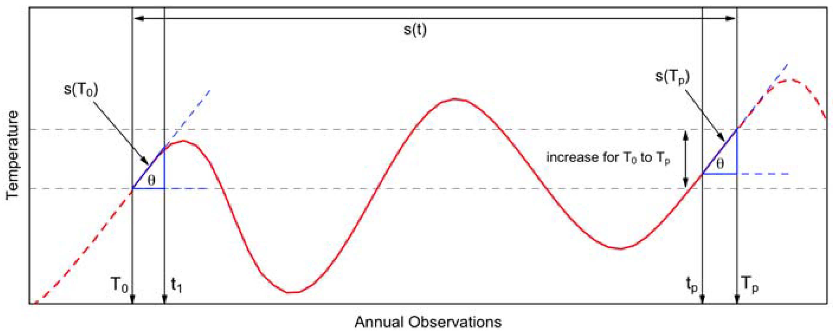
Figure 3.
Adjusted r-squared and cross-validated error for three-sample 1:30 p.m. MODIS LST time series with varying number of knots and their placements.
Figure 3.
Adjusted r-squared and cross-validated error for three-sample 1:30 p.m. MODIS LST time series with varying number of knots and their placements.

Figure 4.
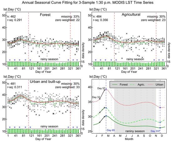
Annual seasonality of three 1:30 p.m. MODIS LST time series with cubic spline fitting (red lines) using eight knots at “best practice” knots location (blue plus) at Julian Days 10, 35, 60, 90, 115, 310, 335 and 355. The green lines connect the average LST values within the Julian day. The “n” label displays the total number of observation used in the seasonal extraction process. The “missing” label indicates the percentage of missing values. The crosses indicate all the outliers excluded from the cubic spline fitting, and the total number of detached observations is displayed as “zero weighted”. The green bar presents the data distribution density. The “r-sq” label shows the adjusted r-squared value of the cubic spline function fitted to the data. The dark (black) dots indicate high-quality LST data, and the dots turn pale (grey) when the LST data are subjected to data quality control.
Figure 4.
Annual seasonality of three 1:30 p.m. MODIS LST time series with cubic spline fitting (red lines) using eight knots at “best practice” knots location (blue plus) at Julian Days 10, 35, 60, 90, 115, 310, 335 and 355. The green lines connect the average LST values within the Julian day. The “n” label displays the total number of observation used in the seasonal extraction process. The “missing” label indicates the percentage of missing values. The crosses indicate all the outliers excluded from the cubic spline fitting, and the total number of detached observations is displayed as “zero weighted”. The green bar presents the data distribution density. The “r-sq” label shows the adjusted r-squared value of the cubic spline function fitted to the data. The dark (black) dots indicate high-quality LST data, and the dots turn pale (grey) when the LST data are subjected to data quality control.
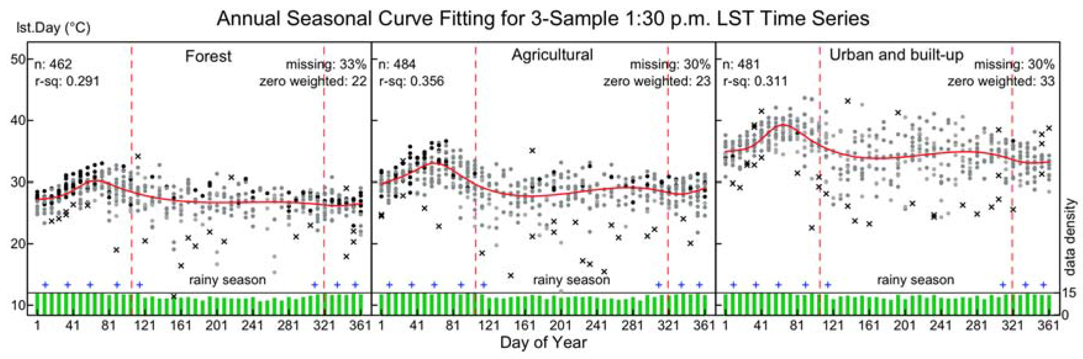
Figure 5.
Trend comparison of seasonality produced from the proposed spline-based seasonality extraction method with the average MODIS LST and 2-m air temperature. The vertical black lines indicate the range of monthly average maximum and minimum temperature.
Figure 5.
Trend comparison of seasonality produced from the proposed spline-based seasonality extraction method with the average MODIS LST and 2-m air temperature. The vertical black lines indicate the range of monthly average maximum and minimum temperature.
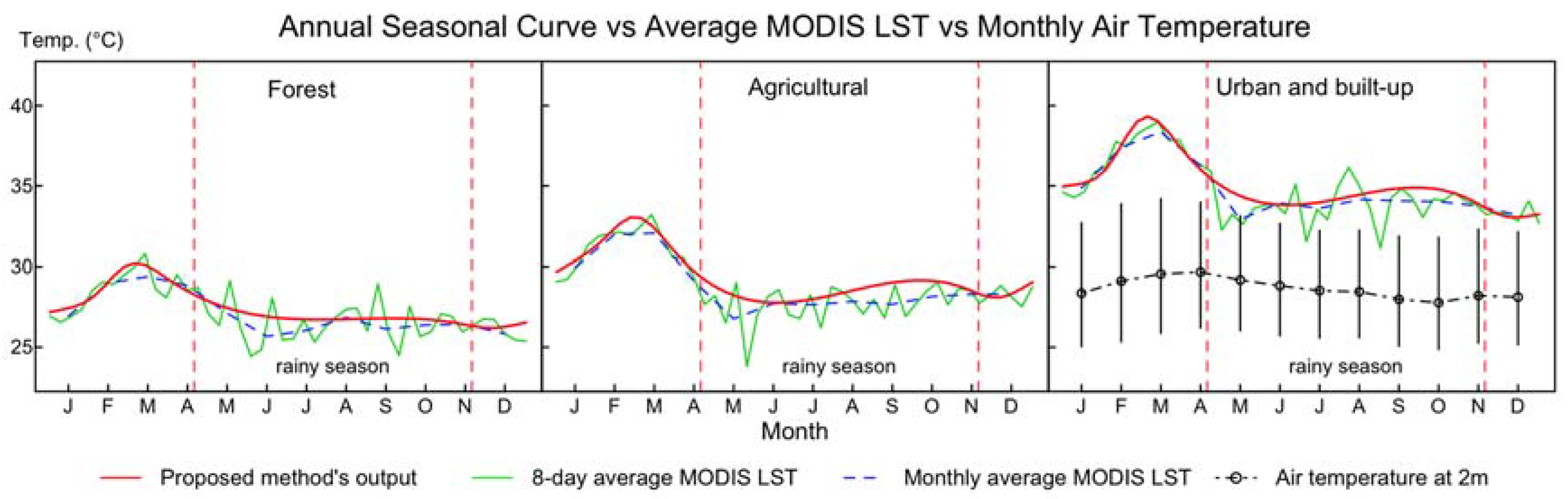
Figure 6.
Seasonality of 1:30 p.m. MODIS LST time series. (a) The seasonal profiles of forest, agricultural and urban land cover classes; (b) relation of seasonal profiles in agricultural and urban land cover to the natural forest.
Figure 6.
Seasonality of 1:30 p.m. MODIS LST time series. (a) The seasonal profiles of forest, agricultural and urban land cover classes; (b) relation of seasonal profiles in agricultural and urban land cover to the natural forest.

Figure 7.
Spatial distribution of MODIS LST trends for the (a) 10:30 a.m. and (b) 1:30 p.m. datasets, including the p-value distribution of their trends, (c,d) for the 10:30 a.m. and 1:30 p.m. datasets, respectively.
Figure 7.
Spatial distribution of MODIS LST trends for the (a) 10:30 a.m. and (b) 1:30 p.m. datasets, including the p-value distribution of their trends, (c,d) for the 10:30 a.m. and 1:30 p.m. datasets, respectively.

Figure 8.
Overall decadal surface temperature trend (error bars denote 95% confidence intervals) in five LULC types and four areas of Phuket Island for 10:30 a.m. and 1:30 p.m. MODIS LST datasets.
Figure 8.
Overall decadal surface temperature trend (error bars denote 95% confidence intervals) in five LULC types and four areas of Phuket Island for 10:30 a.m. and 1:30 p.m. MODIS LST datasets.
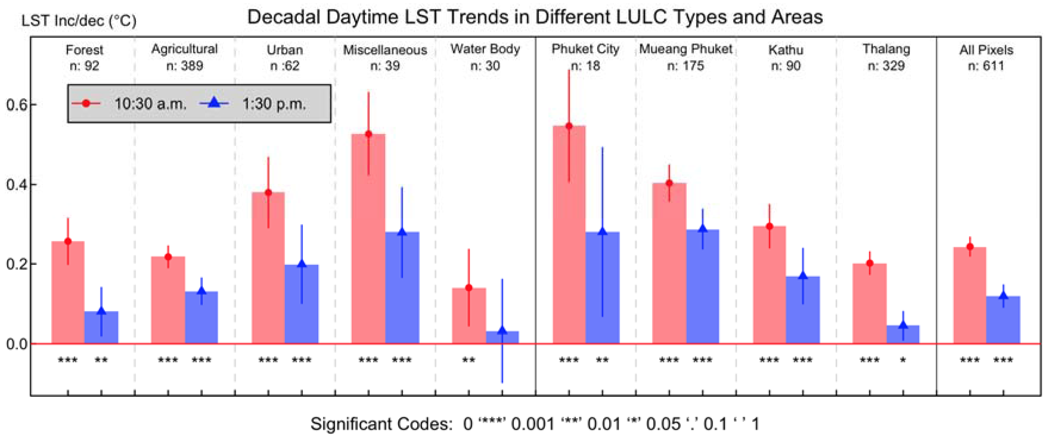
Figure 9.
Plot of cross-correlation function among the seasonality of the three selected study sites. The blue dashed lines represent a 95% confidence interval at ±0.3
Figure 9.
Plot of cross-correlation function among the seasonality of the three selected study sites. The blue dashed lines represent a 95% confidence interval at ±0.3

Table 1.
Details of the district area and its LULC class.
| District | Area: km2 | Lowland: km2 (%) * | LULC 2009: km2 (%) | ||||
|---|---|---|---|---|---|---|---|
| F | A | U | M | W | |||
| Phuket City | 13.6 | 12.6 (92.6) | 0.7 (5.2) | 1.2 (8.8) | 10.8 (79.4) | 0.6 (4.4) | 0.3 (2.2) |
| Mueang Phuket | 151.8 | 102.6 (67.6) | 37.5 (24.6) | 41.4 (27.3) | 58.6 (38.6) | 12.6 (8.4) | 1.6 (1.1) |
| Kathu | 80.2 | 26.0 (32.4) | 28.0 (34.9) | 22.7 (28.3) | 23.8 (29.7) | 4.5 (5.6) | 1.2 (1.5) |
| Thalang | 284.4 | 212.8 (74.8) | 53.8 (18.9) | 165.7 (58.3) | 40.3 (14.2) | 19.7 (6.9) | 4.9 (1.7) |
| Total | 530.0 | 354.0 (66.8) | 120.0 (22.6) | 231.0 (43.6) | 133.5 (25.2) | 37.5 (7.1) | 8.0 (1.5) |
* At altitudes lower than 40 m above the mean sea level and slope less than 15%.
Table 2.
Location of the three study sites and their LULC class.
| Site | Average Elevation | LULC 2009 | MODIS Sinusoidal Project Tile System | Latitude, Longitude (Middle of Pixel) |
|---|---|---|---|---|
| 1 | 275.2 m | Forest (F) | V: 8, H: 27, S: 800, L: 233 | 8.054167, 98.374528 |
| 2 | 53.1 m | Agricultural (A) * | V: 8, H: 27, S: 881, L: 232 | 8.062500, 98.317638 |
| 3 | 14.6 m | Urban and built-up (U) | V: 8, H: 27, S: 895, L: 253 | 7.887500, 98.393357 |
* Only para-rubber plantation; V: Vertical tile, H: Horizontal tile, S: Sample and L: Line.
Table 3.
Cross-correlation coefficients among the seasonality of the three selected study sites.
| Cross-Correlation | Lag | ||||||||||||
|---|---|---|---|---|---|---|---|---|---|---|---|---|---|
| −6 | −5 | −4 | −3 | −2 | −1 | 0 | 1 | 2 | 3 | 4 | 5 | 6 | |
| Forest vs. Agric. | 0.047 | 0.182 | 0.333 | 0.492 | 0.645 | 0.778 | 0.877 | 0.929 | 0.933* | 0.892 | 0.819 | 0.724 | 0.618 |
| Forest vs. Urban | 0.225 | 0.366 | 0.520 | 0.674 | 0.810 | 0.910 | 0.960* | 0.939 | 0.870 | 0.765 | 0.641 | 0.514 | 0.395 |
| Urban vs. Agric. | 0.101 | 0.241 | 0.397 | 0.560 | 0.714 | 0.843 | 0.931 | 0.963* | 0.936 | 0.859 | 0.744 | 0.607 | 0.462 |
* maximum correlation coefficient for the pair of seasonality from the study sites.
© 2017 by the authors. Licensee MDPI, Basel, Switzerland. This article is an open access article distributed under the terms and conditions of the Creative Commons Attribution (CC BY) license (http://creativecommons.org/licenses/by/4.0/).
Share and Cite
MDPI and ACS Style
Wongsai, N.; Wongsai, S.; Huete, A.R. Annual Seasonality Extraction Using the Cubic Spline Function and Decadal Trend in Temporal Daytime MODIS LST Data. Remote Sens. 2017, 9, 1254. https://doi.org/10.3390/rs9121254
AMA Style
Wongsai N, Wongsai S, Huete AR. Annual Seasonality Extraction Using the Cubic Spline Function and Decadal Trend in Temporal Daytime MODIS LST Data. Remote Sensing. 2017; 9(12):1254. https://doi.org/10.3390/rs9121254
Chicago/Turabian StyleWongsai, Noppachai, Sangdao Wongsai, and Alfredo R. Huete. 2017. "Annual Seasonality Extraction Using the Cubic Spline Function and Decadal Trend in Temporal Daytime MODIS LST Data" Remote Sensing 9, no. 12: 1254. https://doi.org/10.3390/rs9121254
Note that from the first issue of 2016, this journal uses article numbers instead of page numbers. See further details here.