Extreme Sparse Multinomial Logistic Regression: A Fast and Robust Framework for Hyperspectral Image Classification

 , ,
, ,
Abstract
:
1. Introduction
2. Materials and Methods
2.1. The Study Datasets
- (1)
- The Indian Pines dataset: The HSI image was acquired by the AVRIS sensor in 1992. The image contains 145 × 145 pixels and 200 spectral bands after removing 20 bands influenced by the atmospheric affection. There are 10,366 labelled samples in 16 classes within the HSI dataset.
- (2)
- The Pavia University dataset: The system was built by the University of Pavia of Italy in 2001. The Pavia University dataset was acquired by the ROSIS instrument. The image contains 610 × 340 pixels and 103 bands after discarding 12 noisy and water absorption bands. In total, there are 42776 labelled samples in 9 classes within this dataset.
2.2. Review of EMAPs
2.3. Review of SMLR
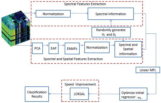
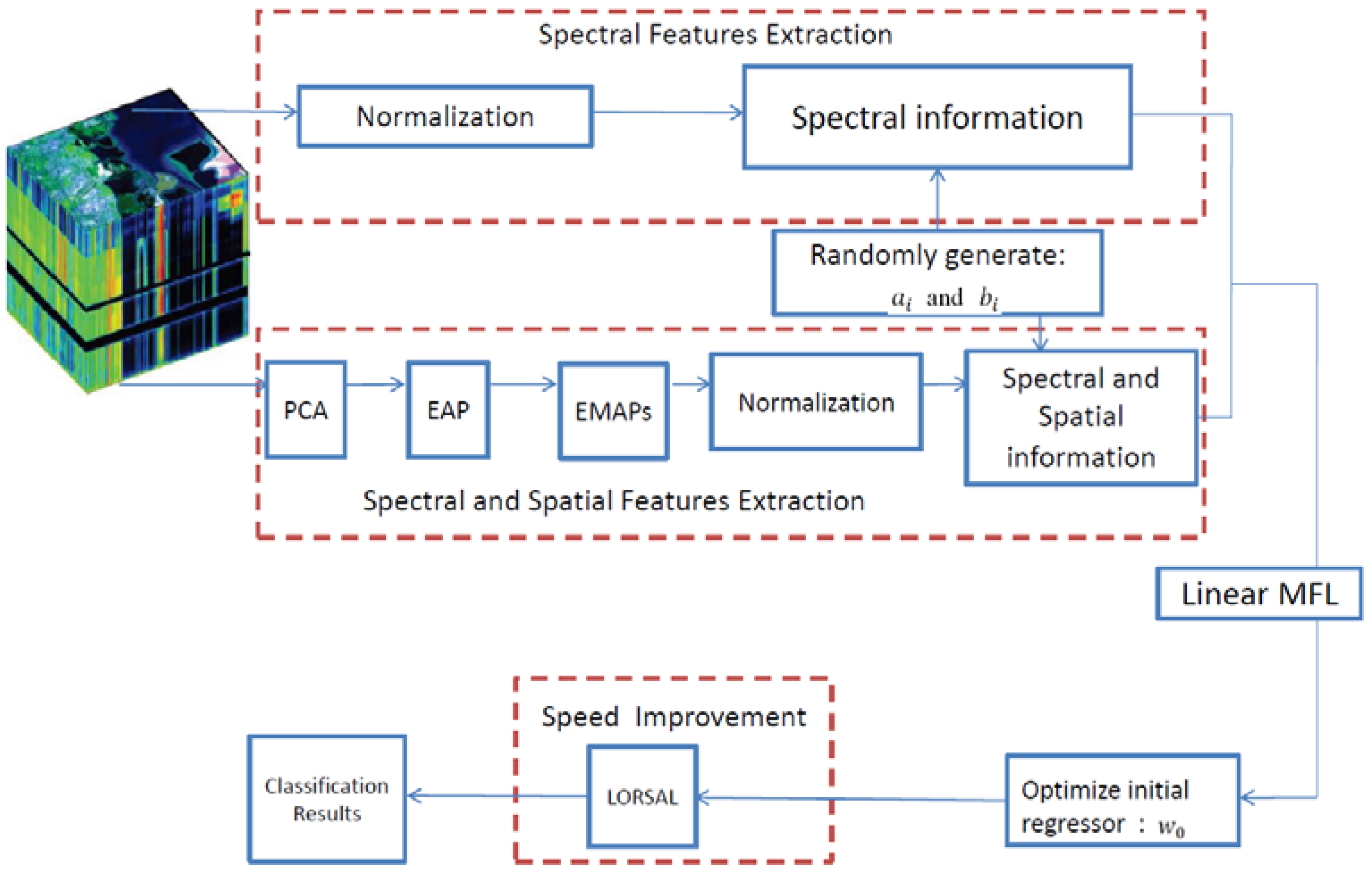
2.4. The Proposed ESMLR Framework
- (1)
- Linear function: ;
- (2)
- Sigmoid function: ;
- (3)
- Gaussian function: ;
- (4)
- Hardlimit function: ;
- (5)
- Multiquadrics function: , etc.
2.5. ESMLR with A Linear MFL
3. Experimental Results and Discussion
3.1. Compared Methods and Parameter Settings
- (1)
- Overall accuracy (OA): The number of correctly classified HSI pixels divided by the total number of test number [47];
- (2)
- Average accuracy (AA): The average value of the classification accuracies of all classes [47];
- (3)
- Kappa coefficient (k): A statistical measurement of agreement between the final classification and the ground-truth map [47].
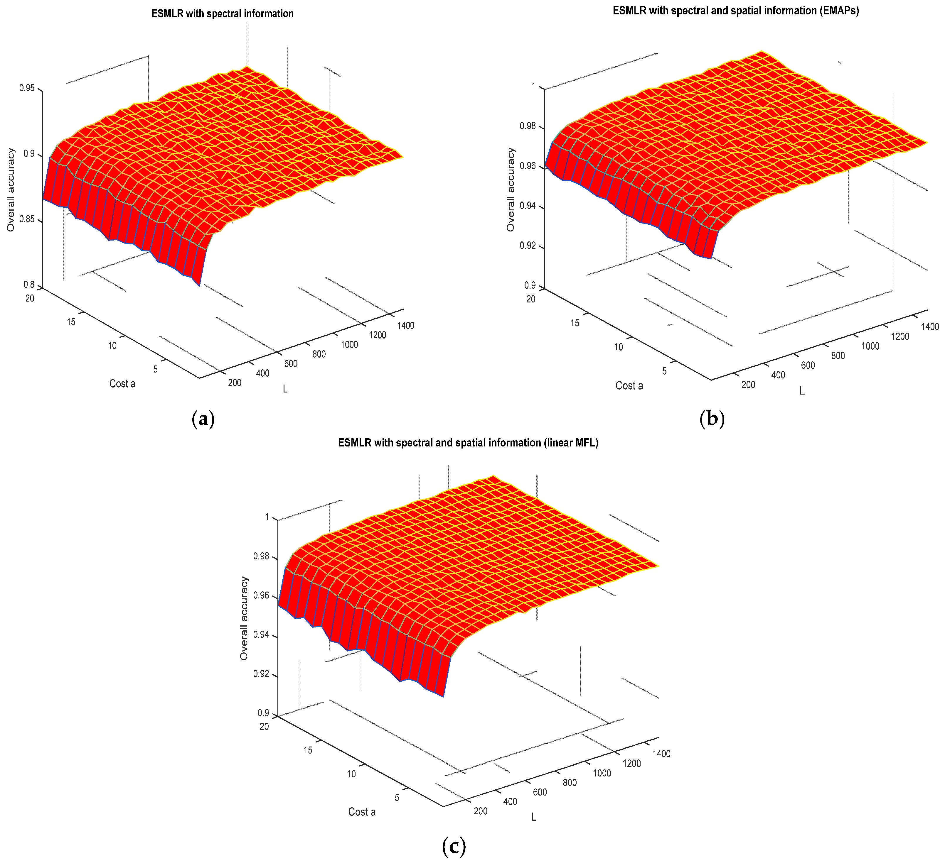
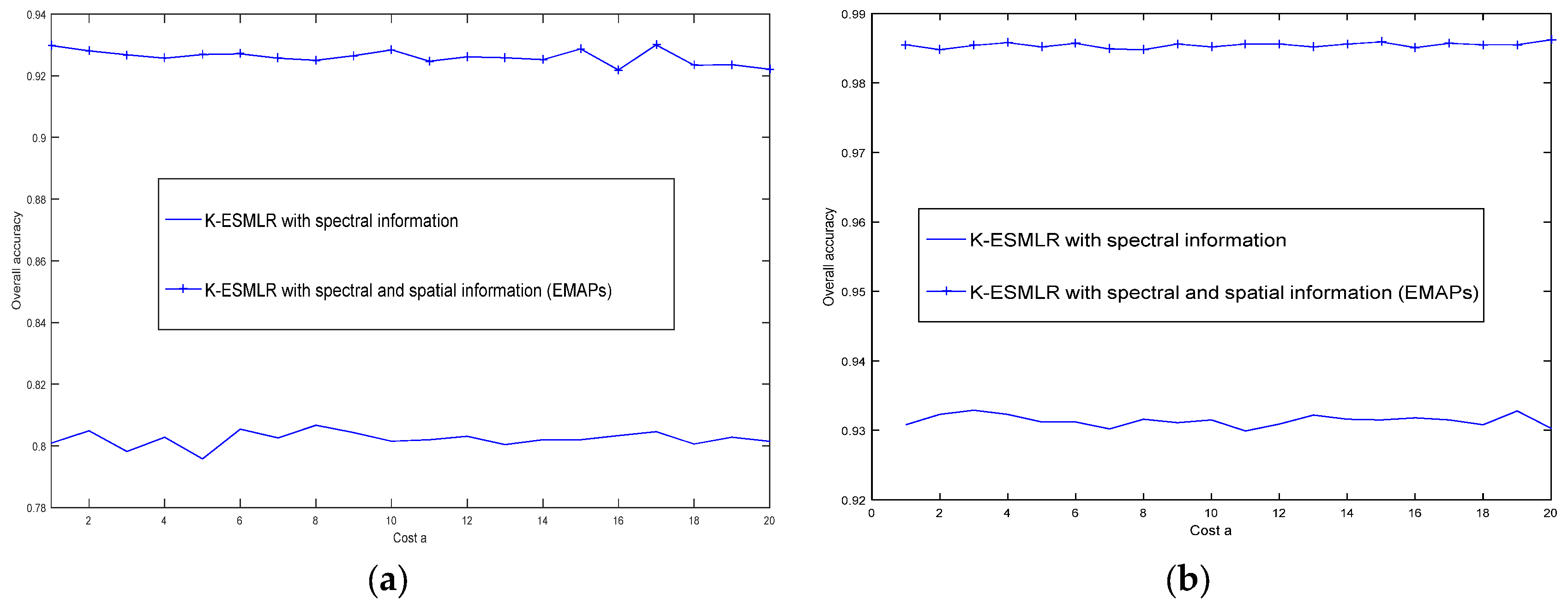
3.2. Discussions on The Robustness of The ESMLR Framework
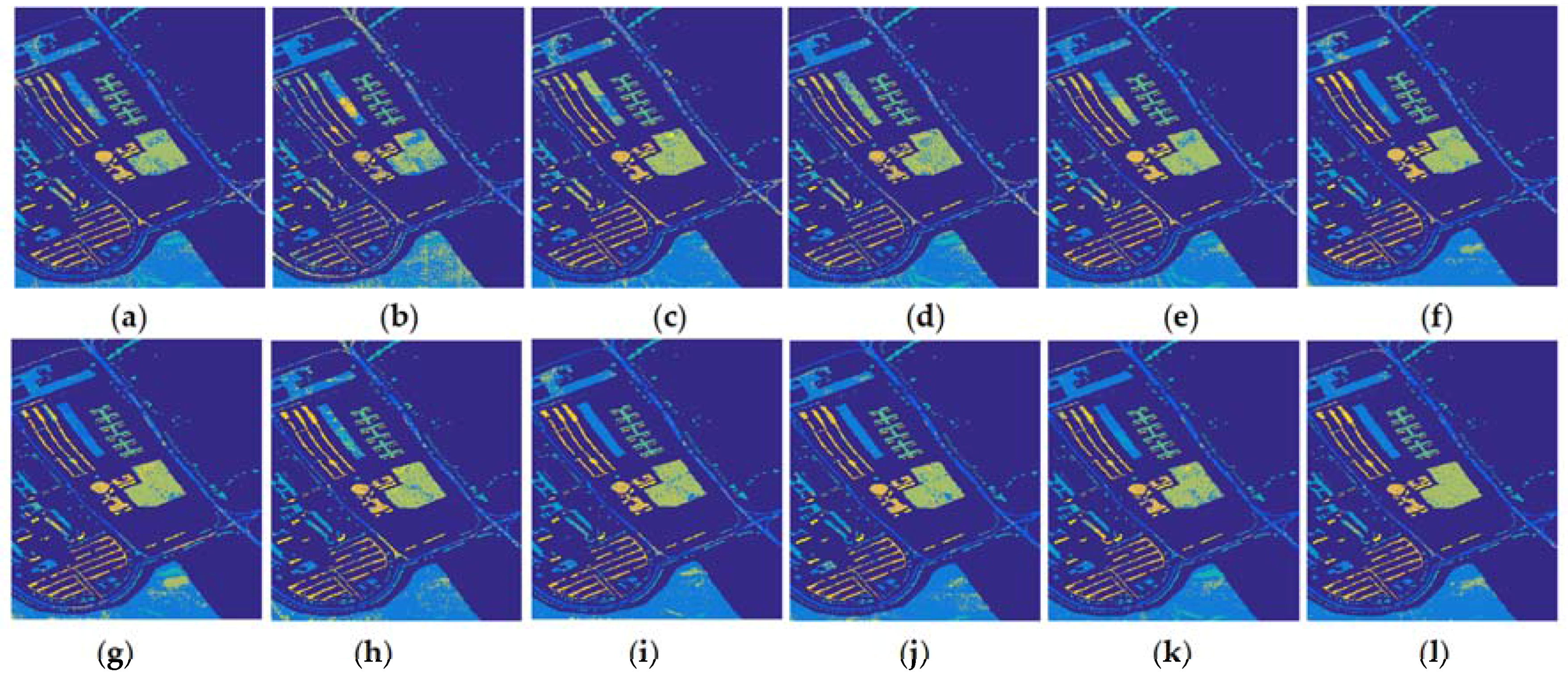
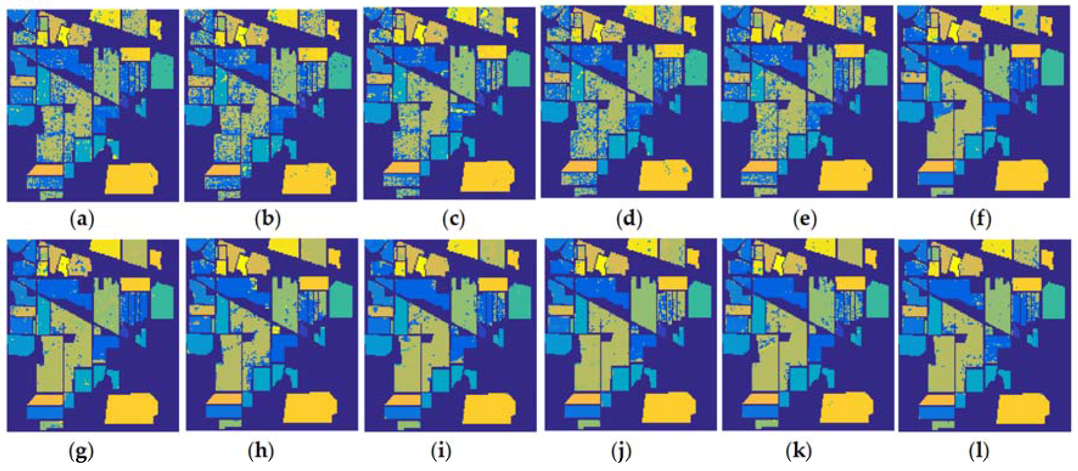
3.3. Discussions on Classification Results and The Running Time of Different Algorithms
- (1)
- Compared with the SMLR, the proposed ESMLR achieves better classification results yet the running time is quite comparable under the aforementioned three different situations. Also, it seems ESMLR has a strong learning ability for a small number of training samples when only spectral information is used. For a class with the classification accuracy less than 60%, the improvement is dramatic. This demonstrates the fast and robustness performance of the proposed framework.
- (2)
- Compared with K-SVM, they achieve better classification results compared to the ESMLR when only the spectral information is used. However, it requires much more computational time than the proposed approach. When both the spectral and spatial information was used, the proposed ESMLR framework achieves better classification results than K-SVM. This again clearly demonstrates the robustness and efficiency of the proposed framework.
3.4. Classification Results with Different Numbers of Training Samples
3.5. Comparing the Proposed ESMLR with CNN and Recurrent Neural Networks (RNN)
4. Conclusions
Acknowledgments
Author Contributions
Conflicts of Interest
Appendix A

| - | Predicted- | ||||||||||||||||
|---|---|---|---|---|---|---|---|---|---|---|---|---|---|---|---|---|---|
| Actually | Class | 1 | 2 | 3 | 4 | 5 | 6 | 7 | 8 | 9 | 10 | 11 | 12 | 13 | 14 | 15 | 16 |
| 1 | 44.9 | 1.5 | 0 | 0 | 1.2 | 0.2 | 0 | 0 | 0.1 | 1.3 | 0.9 | 0.9 | 0 | 0 | 0 | 0 | |
| 2 | 0 | 1223.9 | 15.6 | 2 | 0.2 | 1.4 | 0 | 0 | 0.8 | 30.3 | 86.3 | 1.8 | 0 | 0.1 | 0.6 | 0 | |
| 3 | 0 | 28.3 | 742 | 6.8 | 0.1 | 0 | 0 | 0 | 0.4 | 5.3 | 5.9 | 4.2 | 0 | 0 | 0 | 0 | |
| 4 | 0.1 | 6.3 | 7.6 | 185.9 | 0.6 | 0 | 0 | 0 | 0.3 | 7.7 | 6.3 | 8.10 | 0 | 0.1 | 0 | 0 | |
| 5 | 0.3 | 3.3 | 1.5 | 1.8 | 433.8 | 11.4 | 5.4 | 0 | 0 | 6.5 | 2.5 | 6.1 | 0 | 0 | 0.4 | 0 | |
| 6 | 0 | 0.6 | 0 | 1.5 | 0.8 | 702.2 | 0 | 0 | 0.1 | 2.1 | 1.1 | 0.1 | 0 | 0.1 | 1.4 | 0 | |
| 7 | 0.2 | 0 | 0 | 0 | 0.8 | 0.1 | 21.7 | 0 | 0 | 0.2 | 0 | 0 | 0 | 0 | 0 | 0 | |
| 8 | 0 | 1.1 | 0 | 0 | 0.5 | 0.3 | 0 | 461.6 | 0 | 0.1 | 0.6 | 0.7 | 0 | 0 | 0.1 | 0 | |
| 9 | 0 | 0 | 0.9 | 0.2 | 0 | 0 | 0 | 0 | 15.3 | 0 | 0.6 | 0 | 0 | 0 | 0 | 0 | |
| 10 | 0 | 31.6 | 2.3 | 0.5 | 0.6 | 2.9 | 0 | 0 | 0.2 | 808.4 | 55 | 18.5 | 0 | 0 | 0 | 0 | |
| 11 | 0.3 | 52.5 | 2.8 | 0.3 | 0.8 | 1.5 | 0 | 0 | 0.4 | 52.5 | 2228.8 | 5 | 0 | 0 | 0.1 | 0 | |
| 12 | 0 | 6.4 | 13.2 | 6.4 | 1.1 | 0.4 | 0 | 0 | 0.2 | 32.4 | 13.3 | 508 | 0 | 0 | 1.2 | 1.4 | |
| 13 | 0 | 0 | 0.4 | 0 | 0 | 0 | 0 | 0 | 0.2 | 0.3 | 0.1 | 0 | 201 | 0 | 0 | 0 | |
| 14 | 0 | 0 | 0.3 | 0 | 0 | 3.5 | 0 | 0 | 0 | 0.4 | 0.4 | 0.2 | 0 | 1222.9 | 2.3 | 0 | |
| 15 | 0.7 | 7.6 | 2.8 | 0.2 | 6.0 | 1.5 | 0.7 | 0 | 0.2 | 2.8 | 3.3 | 4.6 | 1.6 | 2.7 | 326.3 | 0 | |
| 16 | 0 | 3.7 | 1.6 | 1.6 | 1.9 | 0 | 0 | 0 | 0.1 | 1.4 | 6 | 3.3 | 0 | 0.2 | 0 | 71.2 | |
| - | Predicted | |||||||||
|---|---|---|---|---|---|---|---|---|---|---|
| Actually | Class | 1 | 2 | 3 | 4 | 5 | 6 | 7 | 8 | 9 |
| 1 | 5957.2 | 5.2 | 33.6 | 0.1 | 0 | 9 | 50.8 | 27.1 | 0 | |
| 2 | 2.3 | 17934.3 | 1.5 | 40.5 | 0 | 124.7 | 0.4 | 5.3 | 0 | |
| 3 | 3.8 | 1.1 | 1648.1 | 0 | 0 | 0 | 1.1 | 52.9 | 0 | |
| 4 | 1.5 | 11.3 | 3.6 | 2515.9 | 0 | 2.2 | 1.6 | 3.9 | 0 | |
| 5 | 2.5 | 0.4 | 1.4 | 0 | 1068.9 | 0.7 | 1.7 | 4.4 | 0 | |
| 6 | 3.9 | 27.3 | 3.1 | 0.2 | 0 | 4434.8 | 0.8 | 26.9 | 0 | |
| 7 | 13.6 | 0 | 0.6 | 0 | 0 | 0.2 | 940.5 | 0.1 | 0 | |
| 8 | 8.7 | 0.3 | 49.1 | 0 | 0 | 8.1 | 1.6 | 3100.2 | 0 | |
| 9 | 1.2 | 0.1 | 0.7 | 0 | 0 | 0.5 | 0.8 | 1.1 | 711.6 | |
Appendix B
- (1)
- H0: There are no salient difference between SMLR-linear MFL and EMSLR-linear MFL in term of OA;H1: There are salient difference between SMLR and ESMLR in term of OA, reject hypothesis H0.
- (2)
- H0: There are no salient difference between SVM-EMAPs and the proposed EMSLR-linear MFL in term of OA;H1: There are salient difference between SVM-EMAPs and the proposed ESMLR-linear MFL in term of OA, reject H0.
| Indian Pines Dataset | Pavia University Dataset | |||||||||
|---|---|---|---|---|---|---|---|---|---|---|
| i | ||||||||||
| sgn | abs | Ri | sgn( | |||||||
| 1 | 90.5370 | 89.6000 | 1 | 0.9370 | 13 | 13 | 89.8326 | 90.8077 | 90.9727 | 91.9417 |
| 2 | 92.7624 | 91.3100 | 1 | 1.4524 | 10 | 10 | 89.8326 | 93.2549 | 89.4710 | 92.0360 |
| 3 | 92.8236 | 89.3500 | 1 | 3.4736 | 1 | 1 | 89.1078 | 92.8541 | 89.0607 | 88.9004 |
| 4 | 90.0980 | 89.9200 | 1 | 0.1780 | 19 | 19 | 87.2805 | 89.9967 | 89.8387 | 93.1535 |
| 5 | 92.9563 | 90.7500 | 1 | 2.2063 | 6 | 6 | 88.6382 | 92.3590 | 91.4537 | 91.7696 |
| 6 | 91.4047 | 89.2800 | 1 | 2.1247 | 8 | 8 | 89.1793 | 92.1822 | 88.3369 | 90.6568 |
| 7 | 90.1388 | 89.2900 | 1 | 0.8488 | 14 | 14 | 88.9955 | 92.7622 | 87.2525 | 92.9107 |
| 8 | 92.3438 | 89.7000 | 1 | 2.6438 | 4 | 4 | 85.5349 | 89.4285 | 86.2693 | 88.7825 |
| 9 | 91.2617 | 90.8700 | 1 | 0.3917 | 16 | 16 | 88.3932 | 92.1893 | 90.3928 | 86.2434 |
| 10 | 92.1294 | 90.6900 | 1 | 1.4394 | 11 | 11 | 87.2805 | 93.0592 | 90.8054 | 89.7232 |
| 11 | 91.7211 | 91.7700 | -1 | 0.0489 | 20 | -20 | 89.1180 | 93.0993 | 92.5028 | 91.2392 |
| 12 | 92.8440 | 90.8600 | 1 | 1.9840 | 9 | 9 | 89.7407 | 93.7217 | 87.6273 | 87.9597 |
| 13 | 93.0073 | 89.7100 | 1 | 3.2973 | 2 | 2 | 88.1993 | 93.9457 | 90.1617 | 89.5676 |
| 14 | 90.3328 | 90.0100 | 1 | 0.3228 | 18 | 18 | 88.0870 | 93.1064 | 89.2776 | 91.1543 |
| 15 | 91.1188 | 92.3600 | 1 | 1.2412 | 12 | 12 | 89.7305 | 93.1182 | 91.0576 | 89.9330 |
| 16 | 91.5680 | 88.7800 | -1 | 2.7880 | 3 | -3 | 90.8942 | 91.7177 | 87.8489 | 90.6002 |
| 17 | 92.0682 | 89.8800 | 1 | 2.1882 | 7 | 7 | 89.4345 | 92.9272 | 90.5602 | 89.0301 |
| 18 | 91.3842 | 90.9400 | 1 | 0.4442 | 15 | 15 | 87.9543 | 93.4812 | 91.7673 | 90.4800 |
| 19 | 92.8644 | 90.5100 | 1 | 2.3544 | 5 | 5 | 88.8220 | 90.8148 | 91.3948 | 92.1374 |
| 20 | 91.1801 | 91.5100 | 1 | 0.3299 | 17 | 17 | 87.8216 | 90.4894 | 89.6407 | 90.6238 |
| Av | 91.7272 | 90.3545 | - | - | - | - | 88.6939 | 92.2658 | 89.7846 | 90.4422 |
References
- Plaza, A.; Benediktsson, J.A.; Boardman, J.W.; Brazile, J.; Bruzzone, L.; Camps-Valls, G.; Chanussot, J.; Fauvel, M.; Gamba, P.; Gualtieri, A.; et al. Recent advances in techniques for hyperspectral image processing. Remote Sens. Environ. 2009, 113, S110–S122. [Google Scholar] [CrossRef]
- Li, J.; Marpu, P.R.; Plaza, A.; Bioucas-Dias, J.M. Generalized composite kernel framework for hyperspectral image classification. IEEE Trans. Geosci. Remote Sens. 2013, 51, 4816–4829. [Google Scholar] [CrossRef]
- Hughes, G. On the mean accuracy of statistical pattern recognizers. IEEE Trans. Inf. Theory 1968, 14, 55–63. [Google Scholar] [CrossRef]
- Yu, H.; Gao, L.; Li, J.; Li, S.S.; Zhang, B.; Benediktsson, J.A. Spectral-Spatial Hyperspectral Image Classification Using Subspace-Based Support Vector Machines and Adaptive Markov Random Fields. Remote Sens. 2016, 8, 355. [Google Scholar] [CrossRef]
- Fang, L.; Li, S.; Duan, W.; Ren, J.; Atli Benediktsson, J. Classification of hyperspectral images by exploiting spectral-spatial information of superpixel via multiple kernels. IEEE Trans. Geosci. Remote Sens. 2015, 53, 6663–6674. [Google Scholar] [CrossRef]
- Samat, A.; Du, P.; Liu, S.; Li, J.; Cheng, L. Ensemble Extreme Learning Machines for Hyperspectral Image Classification. IEEE J. Sel. Top. Appl. Earth Obs. Remote Sens. 2014, 7, 1060–1069. [Google Scholar] [CrossRef]
- Li, J.; Huang, X.; Gamba, P.; Bioucas-Dias, J.M.; Zhang, L.; Benediktsson, J.A.; Plaza, A. Multiple feature learning for hyperspectral image classification. IEEE Trans. Geosci. Remote Sens. 2015, 53, 1592–1606. [Google Scholar] [CrossRef]
- Li, J.; Bioucas-Dias, J.M.; Plaza, A. Spectral–spatial hyperspectral image segmentation using subspace multinomial logistic regression and Markov random fields. IEEE Trans. Geosci. Remote Sens. 2012, 50, 809–823. [Google Scholar] [CrossRef]
- Li, J.; Bioucas-Dias, J.M.; Plaza, A. Semisupervised hyperspectral image segmentation using multinomial logistic regression with active learning. IEEE Trans. Geosci. Remote Sens. 2010, 48, 4085–4098. [Google Scholar] [CrossRef]
- Li, C.; Ma, Y.; Mei, X.; Liu, C.; Ma, J. Hyperspectral Unmixing with Robust Collaborative Sparse Regression. Remote Sens. 2016, 8, 588. [Google Scholar] [CrossRef]
- Ren, J.; Zabalza, Z.; Marshall, S.; Zheng, J. Effective feature extraction and data reduction with hyperspectral imaging in remote sensing. IEEE Signal Proc. Mag. 2014, 31, 149–154. [Google Scholar] [CrossRef]
- Kasun, L.L.C.; Yang, Y.; Huang, G.B.; Zhang, Z. Dimension Reduction with Extreme Learning Machine. IEEE Trans. Image Process. 2016, 25, 3906–3918. [Google Scholar] [CrossRef] [PubMed]
- Zabalza, J.; Ren, J.; Liu, Z.; Marshall, S. Structured covaciance principle component analysis for real-time onsite feature extraction and dimensionality reduction in hyperspectral imaging. Appl. Opt. 2014, 53, 4440–4449. [Google Scholar] [CrossRef] [PubMed]
- Zabalza, J.; Ren, J.; Yang, M.; Zhang, Y.; Wang, J.; Marshall, S.; Han, J. Novel Folded-PCA for Improved Feature Extraction and Data Reduction with Hyperspectral Imaging and SAR in Remote Sensing. ISPRS J. Photogramm. Remote Sens. 2014, 93, 112–122. [Google Scholar] [CrossRef] [Green Version]
- Dalla Mura, M.; Villa, A.; Benediktsson, J.A.; Chanussot, J.; Bruzzone, L. Classification of hyperspectral images by using extended morphological attribute profiles and independent component analysis. IEEE Geosci. Remote Sens. Lett. 2011, 8, 542–546. [Google Scholar] [CrossRef]
- Dalla Mura, M.; Benediktsson, J.A.; Waske, B.; Bruzzone, L. Morphological attribute profiles for the analysis of very high resolution images. IEEE Trans. Geosci. Remote Sens. 2010, 48, 3747–3762. [Google Scholar] [CrossRef]
- Dalla Mura, M.; Atli Benediktsson, J.; Waske, B.; Bruzzone, L. Extended profiles with morphological attribute filters for the analysis of hyperspectral data. Int. J. Remote Sens. 2010, 31, 5975–5991. [Google Scholar] [CrossRef]
- Qiao, T.; Ren, J.; Wang, Z.; Zabalza, J.; Sun, M.; Zhao, H.; Li, S.; Benediktsson, J.A.; Dai, Q.; Marshall, S. Effective denoising and classification of hyperspectral images using curvelet transform and singular spectrum analysis. IEEE Trans. Geosci. Remote Sens. 2017, 55, 119–133. [Google Scholar] [CrossRef]
- Zabalza, J.; Ren, J.; Zheng, J.; Han, J.; Zhao, H.; Li, S.; Marshall, S. Novel two dimensional singular spectrum analysis for effective feature extraction and data classification in hyperspectral imaging. IEEE Trans. Geosci. Remote Sens. 2015, 53, 4418–4433. [Google Scholar] [CrossRef]
- Qiao, T.; Ren, J.; Craigie, C.; Zabalza, Z.; Maltin, C.; Marshall, S. Singular spectrum analysis for improving hyperspectral imaging based beef eating quality evaluation. Comput. Electron. Agric. 2015, 115, 21–25. [Google Scholar] [CrossRef]
- Zabalza, J.; Ren, J.; Wang, Z.; Zhao, H.; Wang, J.; Marshall, S. Fast implementation of singular spectrum analysis for effective feature extraction in hyperspectral imaging. IEEE J. Sel. Top. Appl. Earth Obs. Remote Sens. 2015, 8, 2845–2853. [Google Scholar] [CrossRef]
- Zabalza, J.; Ren, J.; Zheng, J.; Zhao, H.; Qing, C.; Yang, Z.; Du, P.; Marshall, S. Novel segmented stacked autoencoder for effective dimensionality reduction and feature extraction in hyperspectral imaging. Neurocomputing 2016, 185, 1–10. [Google Scholar] [CrossRef] [Green Version]
- Krishnapuram, B.; Carin, L.; Figueiredo, M.A.T.; Hartemink, A.J. Sparse multinomi al logistic regression: Fast algorithms and generalization bounds. IEEE Trans. Pattern Anal. Mach. Intell. 2005, 27, 957–968. [Google Scholar] [CrossRef] [PubMed]
- Bohning, D. Multinomial logistic regression algorithm. Ann. Inst. Stat. Math. 1992, 44, 197–200. [Google Scholar] [CrossRef]
- Zhong, P.; Wang, R. Modeling and classifying hyperspectral imagery by CRFs with sparse higher order potentials. IEEE Trans. Geosci. Remote Sens. 2011, 49, 688–705. [Google Scholar] [CrossRef]
- Sun, L.; Wu, Z.; Liu, J.; Xiao, L.; Wei, Z. Supervised spectral–spatial hyperspectral image classification with weighted Markov random fields. IEEE Trans. Geosci. Remote Sens. 2015, 53, 1490–1503. [Google Scholar] [CrossRef]
- Wu, Z.; Wang, Q.; Plaza, A.; Li, J.; Sun, L.; Wei, Z. Real-Time Implementation of the Sparse Multinomial Logistic Regression for Hyperspectral Image Classification on GPUs. IEEE Geosci. Remote Sens. Lett. 2015, 12, 1456–1460. [Google Scholar]
- Fukushima, K. Neocognitron: A hierarchical neural network capable of visual pattern recognition. Neural Netw. 1988, 1, 119–130. [Google Scholar] [CrossRef]
- Makantasis, K.; Karantzalos, K.; Doulamis, A.; Doulamis, N. Deep supervised learning for hyperspectral data classification through convolutional neural networks. In Proceedings of the 2015 IEEE International Geoscience and Remote Sensing Symposium (IGARSS), Milan, Italy, 26–31 July 2015; pp. 4959–4962. [Google Scholar]
- Huang, G.B.; Zhu, Q.Y.; Siew, C.K. Extreme learning machine: A new learning scheme of feedforward neural networks. In Proceedings of the 2004 IEEE International Joint Conference on Neural Networks, Budapest, Hungary, 25–29 July 2004; pp. 985–990. [Google Scholar]
- Huang, G.B.; Zhou, H.; Ding, X.; Zhang, R. Extreme learning machine for regression and multiclass classification. IEEE Trans. Syst. Man Cybern. Syst. 2012, 42, 513–529. [Google Scholar] [CrossRef] [PubMed]
- Huang, G.B.; Wang, D.H.; Lan, Y. Extreme learning machines: A survey. Int. J. Mach. Learn. Cybern. 2011, 2, 107–122. [Google Scholar] [CrossRef]
- Bartlett, P.L. The sample complexity of pattern classification with neural networks: The size of the weights is more important than the size of the network. IEEE Trans. Inf. Theory 1998, 44, 525–536. [Google Scholar] [CrossRef] [Green Version]
- Zhou, Y.; Peng, J.; Chen, C.L.P. Extreme learning machine with composite kernels for hyperspectral image classification. IEEE J. Sel. Top. Appl. Earth Obs. Remote Sens. 2015, 8, 2351–2360. [Google Scholar] [CrossRef]
- Goodman, E.; Ventura, D. Spatiotemporal pattern recognition via liquid state machines. In Proceedings of the 2006 IEEE International Joint Conference on Neural Networks, Vancouver, BC, Canada, 16–21 July 2006; pp. 3848–3853. [Google Scholar]
- Rodan, A.; Tino, P. Minimum complexity echo state network. IEEE Trans. Neural Netw. 2011, 22, 131–144. [Google Scholar] [CrossRef] [PubMed]
- Jaeger, H.; Haas, H. Harnessing nonlinearity: Predicting chaotic systems and saving energy in wireless communication. Science 2004, 304, 78–80. [Google Scholar] [CrossRef] [PubMed]
- Li, S.; You, Z.H.; Guo, H.; Luo, X.; Zhao, Z.Q. Inverse-free extreme learning machine with optimal information updating. IEEE Trans. Cybern. 2016, 46, 1229–1241. [Google Scholar] [CrossRef] [PubMed]
- Xia, J.; Dalla Mura, M.; Chanussot, J.; Du, P.; He, X. Random subspace ensembles for hyperspectral image classification with extended morphological attribute profiles. IEEE Trans. Geosci. Remote Sens. 2015, 53, 4768–4786. [Google Scholar] [CrossRef]
- Benediktsson, J.A.; Palmason, J.A.; Sveinsson, J.R. Classification of hyperspectral data from urban areas based on extended morphological profiles. IEEE Trans. Geosci. Remote Sens. 2015, 43, 480–491. [Google Scholar] [CrossRef]
- Pedergnana, M.; Marpu, P.R.; Dalla Mura, M.; Benediktsson, J.A.; Bruzzone, L. Classification of remote sensing optical and LiDAR data using extended attribute profiles. IEEE J. Sel. Top. Signal Process. 2012, 6, 856–865. [Google Scholar] [CrossRef]
- Marpu, P.R.; Pedergnana, M.; Dalla Mura, M.; Benediktsson, J.A.; Bruzzone, L. Automatic generation of standard deviation attribute profiles for spectral–spatial classification of remote sensing data. IEEE Geosci. Remote Sens. Lett. 2013, 10, 293–297. [Google Scholar] [CrossRef]
- Bohning, D.; Lindsay, B.G. Monotonicity of quadratic-approximation algorithms. Ann. Inst. Stat. Math. 1988, 40, 641–663. [Google Scholar] [CrossRef]
- Chen, C.L.P. A rapid supervised learning neural network for function interpolation and approximation. IEEE Trans. Neural Netw. 1996, 7, 1220–1230. [Google Scholar] [CrossRef] [PubMed]
- Bioucas-Dias, J.; Figueiredo, M. Logistic Regression via Variable Splitting and Augmented Lagrangian Tools; Instituto Superior Tecnico, TULisbon: Lisboa, Portugal, 2009. [Google Scholar]
- Chang, C.C.; Lin, C.J. LIBSVM: A library for support vector machines. ACM Trans. Intell. Syst. Technol. (TIST) 2011, 2, 1–27. [Google Scholar] [CrossRef]
- Mou, L.; Ghamisi, P.; Zhu, X.X. Deep Recurrent Neural Networks for Hyperspectral Image Classification. IEEE Geosci. Remote Sens. Lett. 2017, 55, 3639–3655. [Google Scholar] [CrossRef]
- Wilcoxon, F.; Katti, S.K.; Wilcox, R.A. Critical values and probability levels for the Wilcoxon rank sum test and the Wilcoxon signed rank test. Sel. Tables Math. Stat. 1970, 1, 171–259. [Google Scholar]
- Peng, J.; Chen, H.; Zhou, Y.; Li, L. Ideal Regularized Composite Kernel for Hyperspectral Image Classification. IEEE J. Sel. Top. Appl. Earth Obs. Remote Sens. 2017, 10, 1563–1574. [Google Scholar] [CrossRef]
- Grant, M.; Boyd, S. CVX: Matlab Software for Disciplined Convex Programming, version 2.0; CVX Research, Inc.: Austin, TX, USA, 2013. [Google Scholar]


| No | Train | Test | Spectral Information | Spectral and Spatial Information | ||||||||||
|---|---|---|---|---|---|---|---|---|---|---|---|---|---|---|
| EMAPs | Proposed Linear MFL | |||||||||||||
| K-SVM | SMLR | K-SMLR | ESMLR | K-ESMLR | K-SVM | SMLR | K-SMLR | ESMLR | K-ESMLR | SMLR | ESMLR | |||
| 1 | 3 | 51 | 58.04 ± 16.46 | 5.88 ± 4.98 | 35.10 ± 14.66 | 17.65 ± 8.77 | 45.10 ± 23.69 | 82.35 ± 27.36 | 87.06 ± 2.48 | 89.41 ± 4.36 | 89.02 ± 3.72 | 87.25 ± 3.10 | 88.04 ± 2.99 | 88.04 ± 2.35 |
| 2 | 71 | 1363 | 77.83 ± 2.25 | 76.00 ± 2.72 | 77.49 ± 3.69 | 75.76 ± 2.82 | 78.02 ± 4.15 | 86.07 ± 2.66 | 86.63 ± 2.10 | 87.33 ± 2.60 | 88.88 ± 2.64 | 88.45 ± 2.00 | 88.82 ± 1.22 | 89.79 ± 1.62 |
| 3 | 41 | 793 | 66.39 ± 5.48 | 45.80 ± 3.80 | 62.24 ± 3.28 | 51.13 ± 4.89 | 62.48 ± 3.61 | 92.85 ± 4.95 | 90.08 ± 4.94 | 95.12 ± 3.45 | 91.95 ± 4.67 | 93.63 ± 3.91 | 89.55 ± 5.79 | 93.57 ± 3.41 |
| 4 | 11 | 223 | 58.43 ± 7.33 | 16.19 ± 4.64 | 44.26 ± 5.01 | 28.07 ± 7.88 | 44.89 ± 11.13 | 80.63 ± 9.44 | 79.87 ± 6.01 | 77.49 ± 9.02 | 79.10 ± 7.22 | 77.98 ± 10.07 | 72.83 ± 5.94 | 83.36 ± 5.26 |
| 5 | 24 | 473 | 89.41 ± 3.26 | 73.57 ± 6.58 | 86.83 ± 5.90 | 80.82 ± 4.81 | 87.61 ± 4.92 | 92.22 ± 4.53 | 90.66 ± 1.70 | 88.77 ± 3.34 | 90.47 ± 4.53 | 92.18 ± 2.89 | 89.05 ± 2.66 | 91.71 ± 4.50 |
| 6 | 37 | 710 | 95.1 ± 1.47 | 94.01 ± 0.71 | 94.20 ± 2.12 | 94.00 ± 2.11 | 95.13 ± 1.11 | 97.52 ± 1.22 | 96.59 ± 1.25 | 98.61 ± 1.02 | 98.13 ± 0.95 | 98.54 ± 1.01 | 97.94 ± 0.70 | 98.90 ± 0.99 |
| 7 | 3 | 23 | 84.78 ± 9.45 | 13.04 ± 7.39 | 33.04 ± 11.26 | 17.39 ± 9.83 | 53.48 ± 9.62 | 94.35 ± 4.12 | 86.09 ± 12.60 | 90.43 ± 7.04 | 90.87 ± 11.68 | 92.61 ± 4.61 | 86.96 ± 0.85 | 94.35 ± 2.10 |
| 8 | 24 | 465 | 97.12 ± 2.00 | 99.55 ± 0.24 | 99.33 ± 0.34 | 99.33 ± 0.51 | 99.14 ± 0.39 | 99.46 ± 0.11 | 99.29 ± 0.54 | 99.40 ± 0.20 | 97.87 ± 0.90 | 99.42 ± 0.45 | 98.97 ± 0.83 | 99.27 ± 0.41 |
| 9 | 3 | 17 | 77.65 ± 14.36 | 3.53 ± 5.68 | 55.88 ± 16.23 | 28.24 ± 11.70 | 79.41 ± 15.25 | 98.82 ± 2.48 | 63.53 ± 23.00 | 81.18 ± 23.98 | 81.18 ± 21.80 | 88.82 ± 20.08 | 67.06 ± 15.74 | 90.00 ± 17.11 |
| 10 | 48 | 920 | 69.25 ± 3.70 | 51.13 ± 4.73 | 66.50 ± 3.12 | 56.63 ± 4.37 | 69.87 ± 4.63 | 83.28 ± 2.71 | 81.60 ± 3.14 | 88.54 ± 1.70 | 88.13 ± 2.65 | 88.96 ± 1.47 | 82.84 ± 2.77 | 87.87 ± 2.54 |
| 11 | 123 | 2345 | 82.52 ± 2.95 | 78.85 ± 2.25 | 82.01 ± 0.99 | 76.44 ± 1.42 | 81.73 ± 1.82 | 93.73 ± 2.38 | 92.59 ± 1.76 | 91.89 ± 2.88 | 94.08 ± 1.46 | 93.25 ± 1.89 | 94.48 ± 1.65 | 95.05 ± 1.55 |
| 12 | 30 | 584 | 75.26 ± 5.99 | 53.83 ± 4.99 | 73.65 ± 4.49 | 60.80 ± 5.30 | 76.46 ± 4.36 | 85.02 ± 5.31 | 74.13 ± 4.84 | 84.28 ± 2.48 | 85.48 ± 4.43 | 85.80 ± 5.82 | 81.87 ± 5.35 | 86.99 ± 4.49 |
| 13 | 10 | 202 | 96.29 ± 2.92 | 96.14 ± 2.46 | 99.36 ± 0.33 | 98.81 ± 1.15 | 99.46 ± 0.37 | 99.36 ± 0.33 | 99.11 ± 0.51 | 99.60 ± 0.21 | 99.46 ± 0.28 | 99.51 ± 0 | 99.01 ± 0.70 | 99.51 ± 0.02 |
| 14 | 64 | 1230 | 95.63 ± 1.60 | 93.24 ± 2.15 | 95.75 ± 1.08 | 93.29 ± 1.40 | 95.46 ± 1.05 | 98.59 ± 0.52 | 99.29 ± 0.98 | 98.92 ± 0.62 | 99.15 ± 0.49 | 99.36 ± 0.21 | 99.49 ± 0.64 | 99.42 ± 0.28 |
| 15 | 19 | 361 | 47.26 ± 5.61 | 52.63 ± 3.97 | 56.79 ± 6.08 | 54.99 ± 5.62 | 59.48 ± 6.80 | 92.96 ± 3.80 | 86.98 ± 6.16 | 90.03 ± 5.45 | 88.25 ± 4.37 | 88.48 ± 5.13 | 87.17 ± 5.07 | 90.39 ± 3.76 |
| 16 | 4 | 91 | 81.54 ± 12.71 | 70.00 ± 5.93 | 56.70 ± 12.15 | 67.14 ± 9.07 | 48.68 ± 13.96 | 93.41 ± 7.80 | 81.10 ± 8.97 | 78.79 ± 10.49 | 71.76 ± 8.79 | 80.55 ± 6.72 | 83.41 ± 9.61 | 78.24 ± 8.67 |
| OA | 80.77 ± 1.02 | 72.57 ± 0.71 | 79.43 ± 1.08 | 74.16 ± 0.80 | 80.18 ± 0.57 | 91.92 ± 1.11 | 90.23 ± 0.65 | 91.93 ± 0.81 | 92.35 ± 0.76 | 92.61 ± 0.70 | 91.42 ± 0.63 | 93.37 ± 0.74 | ||
| AA | 78.28 ± 1.25 | 57.72 ± 1.25 | 69.95 ± 2.02 | 62.53 ± 2.01 | 73.52 ± 2.45 | 91.91 ± 1.94 | 87.16 ± 1.94 | 89.99 ± 1.69 | 89.61 ± 1.55 | 90.92 ± 1.74 | 87.97 ± 1.15 | 91.65 ± 1.07 | ||
| k | 78.01 ± 1.17 | 68.31 ± 0.86 | 76.43 ± 1.26 | 70.30 ± 0.94 | 77.29 ± 0.66 | 90.79 ± 1.27 | 88.85 ± 0.74 | 90.81 ± 0.91 | 91.27 ± 0.87 | 91.57 ± 0.80 | 90.21 ± 0.72 | 92.43 ± 0.85 | ||
| Time(Seconds) | 7.56 | 0.12 | 0.11 | 0.20 | 0.11 | 2.71 | 0.06 | 0.08 | 0.20 | 0.08 | 0.15 | 0.37 | ||
| No. | Train | Test | Spectral Information | Spectral and Spatial Information | ||||||||||
|---|---|---|---|---|---|---|---|---|---|---|---|---|---|---|
| EMAPs | Proposed Linear MFL | |||||||||||||
| K-SVM | SMLR | K-SMLR | ESMLR | K-ESMLR | K-SVM | SMLR | K-SMLR | ESMLR | K-ESMLR | SMLR | ESMLR | |||
| 1 | 548 | 6083 | 90.47 ± 0.87 | 72.84 ± 1.44 | 88.99 ± 1.16 | 87.16 ± 0.71 | 89.577 ± 0.83 | 98.23 ± 0.39 | 90.45 ± 0.55 | 97.77 ± 0.57 | 98.10 ± 0.42 | 98.41 ± 0.27 | 96.73 ± 0.21 | 97.93 ± 0.30 |
| 2 | 540 | 18109 | 94.02 ± 0.54 | 79.2 ± 1.74 | 94.30 ± 0.40 | 92.82 ± 0.74 | 94.366 ± 0.40 | 98.04 ± 0.50 | 92.84 ± 0.55 | 98.68 ± 0.42 | 97.83 ± 0.33 | 98.54 ± 0.31 | 96.67 ± 0.43 | 99.04 ± 0.17 |
| 3 | 392 | 1707 | 84.45 ± 0.43 | 70.91 ± 1.70 | 83.82 ± 1.37 | 80.25 ± 1.10 | 84.28 ± 1.66 | 96.78 ± 0.35 | 83.62 ± 1.38 | 97.06 ± 0.51 | 97.13 ± 0.61 | 97.22 ± 0.52 | 93.16 ± 0.89 | 96.55 ± 0.84 |
| 4 | 524 | 2540 | 97.55 ± 0.47 | 94.98 ± 1.06 | 97.50 ± 0.47 | 97.04 ± 0.27 | 97.53 ± 0.39 | 99.33 ± 0.34 | 97.50 ± 0.59 | 99.06 ± 0.24 | 99.04 ± 0.24 | 99.33 ± 0.32 | 98.34 ± 0.40 | 99.05 ± 0.18 |
| 5 | 265 | 1080 | 99.63 ± 0.28 | 99.48 ± 0.21 | 99.34 ± 0.35 | 99.38 ± 0.33 | 99.23 ± 0.30 | 99.68 ± 0.16 | 99.53 ± 0.28 | 99.58 ± 0.19 | 98.99 ± 0.41 | 99.63 ± 0.14 | 99.56 ± 0.31 | 98.97 ± 0.42 |
| 6 | 532 | 4497 | 94.433 ± 0.92 | 74.75 ± 1.79 | 94.43 ± 0.58 | 92.93 ± 0.65 | 94.38 ± 0.76 | 97.91 ± 0.43 | 93.94 ± 0.31 | 97.97 ± 0.31 | 97.68 ± 0.36 | 98.09 ± 0.47 | 96.90 ± 0.51 | 98.62 ± 0.19 |
| 7 | 375 | 955 | 92.91 ± 1.09 | 77.34 ± 1.90 | 92.73 ± 0.82 | 90.32 ± 1.13 | 93.21 ± 0.833 | 98.12 ± 0.53 | 93.40 ± 1.14 | 98.49 ± 0.55 | 98.20 ± 0.59 | 98.52 ± 0.45 | 96.64 ± 0.98 | 98.48 ± 0.57 |
| 8 | 514 | 3168 | 89.83 ± 1.22 | 75.15 ± 1.05 | 86.10 ± 0.72 | 85.71 ± 1.31 | 88.80 ± 1.16 | 97.94 ± 0.45 | 95.03 ± 0.49 | 98.10 ± 0.26 | 98.22 ± 0.29 | 98.15 ± 0.32 | 96.67 ± 0.40 | 97.86 ± 0.31 |
| 9 | 231 | 716 | 99.86 ± 0.16 | 96.87 ± 0.98 | 99.75 ± 0.18 | 99.41 ± 0.31 | 99.79 ± 0.14 | 99.94 ± 0.12 | 99.75 ± 0.23 | 99.94 ± 0.07 | 99.39 ± 0.32 | 99.94 ± 0.07 | 99.39 ± 0.48 | 99.39 ± 0.26 |
| OA | 93.22 ± 0.38 | 78.88 ± 0.68 | 92.77 ± 0.26 | 91.33 ± 0.38 | 93.133 ± 0.21 | 98.16 ± 0.20 | 93.00 ± 0.25 | 98.41 ± 0.17 | 98.00 ± 0.15 | 98.48 ± 0.15 | 96.79 ± 0.22 | 98.51 ± 0.10 | ||
| AA | 93.68 ± 0.288 | 82.39 ± 0.34 | 93.00 ± 0.22 | 91.67 ± 0.25 | 93.46 ± 0.19 | 98.44 ± 0.12 | 94.01 ± 0.23 | 98.52 ± 0.09 | 98.29 ± 0.14 | 98.65 ± 0.08 | 97.12 ± 0.18 | 98.43 ± 0.09 | ||
| K | 90.83 ± 0.51 | 72.15 ± 0.76 | 90.21 ± 0.344 | 88.30 ± 0.50 | 90.70 ± 0.28 | 97.49 ± 0.27 | 90.55 ± 0.33 | 97.83 ± 0.22 | 97.28 ± 0.20 | 97.93 ± 0.20 | 95.64 ± 0.29 | 98.09 ± 0.12 | ||
| Time (Seconds) | 106.37 | 0.26 | 3.77 | 0.72 | 3.81 | 53.11 | 0.16 | 3.54 | 0.69 | 3.54 | 0.29 | 1.25 | ||
| Spectral Information | Spectral and Spatial Information | ||||||||||||
|---|---|---|---|---|---|---|---|---|---|---|---|---|---|
| EMAPs | Proposed Linear MFL | ||||||||||||
| Q | Index | K-SVM | SMLR | K-SMLR | ESMLR | K-ESMLR | K-SVM | SMLR | K-SMLR | ESMLR | K-ESMLR | SMLR | ESMLR |
| 5 | OA | 51.72 ± 5.53 | 45.09 ± 2.90 | 55.49 ± 2.74 | 53.21 ± 2.77 | 56.54 ± 3.58 | 66.66 ± 4.20 | 68.75 ± 4.52 | 67.61 ± 3.39 | 70.54 ± 2.62 | 69.84 ± 2.66 | 69.20 ± 4.18 | 71.41 ± 2.23 |
| AA | 64.24 ± 4.65 | 57.74 ± 2.17 | 66.65 ± 1.88 | 66.68 ± 1.75 | 68.43 ± 1.88 | 78.48 ± 2.30 | 78.38 ± 2.13 | 78.0 ± 1.85 | 80.31 ± 1.71 | 80.49 ± 1.47 | 78.34 ± 2.26 | 80.60 ± 2.13 | |
| k | 46.23 ± 5.88 | 38.70 ± 2.99 | 50.53 ± 2.86 | 47.93 ± 2.69 | 51.52 ± 3.64 | 62.70 ± 4.51 | 64.95 ± 4.84 | 63.85 ± 3.83 | 66.92 ± 2.86 | 66.07 ± 2.81 | 65.34 ± 4.59 | 67.80 ± 2.52 | |
| 10 | OA | 64.49 ± 2.48 | 53.28 ± 2.03 | 62.52 ± 2.04 | 58.79 ± 3.18 | 63.90 ± 2.29 | 74.94 ± 2.12 | 77.07 ± 2.40 | 77.00 ± 2.17 | 80.67 ± 2.31 | 79.68 ± 2.08 | 77.58 ± 3.54 | 80.33 ± 2.76 |
| AA | 75.84 ± 1.60 | 65.73 ± 1.48 | 73.64 ± 1.12 | 72.44 ± 1.23 | 75.04 ± 1.45 | 84.70 ± 0.90 | 85.08 ± 1.78 | 85.19 ± 1.29 | 86.96 ± 1.57 | 86.90 ± 1.33 | 85.02 ± 1.64 | 87.52 ± 1.74 | |
| k | 60.29 ± 2.75 | 47.77 ± 2.06 | 58.19 ± 2.07 | 54.05 ± 3.32 | 59.51 ± 2.49 | 71.8 ± 2.28 | 74.17 ± 2.67 | 74.23 ± 2.37 | 78.14 ± 2.56 | 77.02 ± 2.34 | 74.72 ± 3.92 | 77.77 ± 3.09 | |
| 15 | OA | 68.68 ± 1.19 | 59.75 ± 2.05 | 66.75 ± 1.18 | 62.34 ± 2.37 | 68.35 ± 1.61 | 80.10 ± 2.04 | 82.00 ± 2.70 | 81.03 ± 1.65 | 83.84 ± 2.10 | 83.22 ± 2.28 | 83.03 ± 2.29 | 84.68 ± 1.22 |
| AA | 78.05 ± 1.16 | 70.61 ± 1.67 | 77.75 ± 0.88 | 75.37 ± 1.08 | 79.21 ± 0.63 | 88.10 ± 1.58 | 88.11 ± 1.31 | 89.01 ± 1.13 | 89.44 ± 1.31 | 89.78 ± 1.20 | 88.97 ± 1.13 | 90.26 ± 0.56 | |
| k | 64.77 ± 1.25 | 54.93 ± 2.17 | 62.83 ± 1.24 | 57.85 ± 2.61 | 64.38 ± 1.63 | 77.51 ± 2.32 | 79.6 ± 2.99 | 78.66 ± 1.81 | 81.69 ± 2.36 | 81.04 ± 2.55 | 80.85 ± 2.52 | 82.66 ± 1.35 | |
| 20 | OA | 71.18 ± 1.81 | 62.55 ± 2.24 | 70.65 ± 1.17 | 65.04 ± 1.48 | 71.44 ± 1.54 | 82.5 ± 2.28 | 86.05 ± 1.26 | 83.40 ± 1.78 | 86.76 ± 1.66 | 85.54 ± 2.11 | 86.51 ± 1.19 | 87.16 ± 1.06 |
| AA | 81.56 ± 1.19 | 72.29 ± 2.37 | 80.67 ± 1.16 | 77.42 ± 0.97 | 81.89 ± 1.24 | 89.88 ± 1.03 | 90.49 ± 0.61 | 90.24 ± 0.90 | 91.64 ± 0.90 | 91.56 ± 0.86 | 90.75 ± 1.21 | 92.08 ± 0.46 | |
| k | 67.66 ± 1.94 | 58.07 ± 2.45 | 67.04 ± 1.26 | 60.80 ± 1.58 | 67.92 ± 1.63 | 80.27 ± 2.51 | 84.14 ± 1.40 | 81.25 ± 1.96 | 84.98 ± 1.88 | 83.63 ± 2.33 | 84.70 ± 1.34 | 85.43 ± 1.18 | |
| 25 | OA | 73.23 ± 1.54 | 63.14 ± 1.56 | 72.04 ± 1.33 | 66.40 ± 1.76 | 74.60 ± 1.71 | 84.23 ± 1.94 | 86.05 ± 1.26 | 86.03 ± 1.76 | 87.67 ± 1.67 | 87.17 ± 1.53 | 86.98 ± 1.53 | 89.45 ± 1.29 |
| AA | 82.27 ± 1.41 | 73.25 ± 1.80 | 81.26 ± 0.79 | 78.00 ± 1.42 | 84.17 ± 1.07 | 90.77 ± 0.68 | 90.49 ± 0.61 | 91.74 ± 1.29 | 92.57 ± 0.88 | 92.73 ± 0.91 | 91.89 ± 0.60 | 93.30 ± 0.71 | |
| k | 70.03 ± 1.71 | 58.77 ± 1.67 | 68.57 ± 1.44 | 62.32 ± 1.92 | 71.35 ± 1.85 | 82.15 ± 2.14 | 84.14 ± 1.40 | 84.18 ± 1.97 | 86.02 ± 1.87 | 85.46 ± 1.71 | 85.23 ± 1.69 | 87.99 ± 1.46 | |
| 30 | OA | 74.57 ± 2.74 | 65.51 ± 1.83 | 72.95 ± 1.84 | 67.70 ± 0.76 | 75.20 ± 1.19 | 86.22 ± 2.29 | 86.65 ± 1.71 | 87.38 ± 1.02 | 89.10 ± 0.97 | 88.79 ± 1.05 | 88.81 ± 1.95 | 89.96 ± 1.74 |
| AA | 83.49 ± 1.31 | 74.36 ± 1.62 | 82.62 ± 1.07 | 78.59 ± 1.60 | 84.2 ± 1.25 | 92.32 ± 1.25 | 90.77 ± 1.07 | 92.55 ± 0.55 | 93.18 ± 0.58 | 93.34 ± 0.45 | 92.66 ± 0.80 | 93.89 ± 0.64 | |
| k | 71.37 ± 2.94 | 61.38 ± 2.00 | 69.61 ± 1.95 | 63.73 ± 0.83 | 71.99 ± 1.32 | 84.38 ± 2.57 | 84.83 ± 1.91 | 85.68 ± 1.13 | 87.60 ± 1.09 | 87.25 ± 1.18 | 87.26 ± 2.16 | 88.58 ± 1.94 | |
| 35 | OA | 76.31 ± 1.54 | 65.96 ± 2.47 | 75.47 ± 1.37 | 69.28 ± 2.08 | 76.37 ± 0.87 | 87.37 ± 1.70 | 88.65 ± 0.94 | 88.32 ± 1.44 | 90.29 ± 1.44 | 89.72 ± 1.19 | 89.93 ± 1.40 | 91.22 ± 0.76 |
| AA | 84.71 ± 1.07 | 74.72 ± 2.29 | 83.93 ± 1.64 | 79.89 ± 1.53 | 85.53 ± 0.65 | 92.80 ± 0.81 | 92.23 ± 0.78 | 93.26 ± 0.81 | 93.60 ± 0.50 | 93.71 ± 0.45 | 93.35 ± 0.83 | 94.74 ± 0.58 | |
| k | 73.23 ± 1.71 | 61.89 ± 2.67 | 72.31 ± 1.49 | 65.42 ± 2.23 | 73.31 ± 0.96 | 85.65 ± 1.91 | 87.04 ± 1.06 | 86.74 ± 1.61 | 88.94 ± 1.61 | 88.30 ± 1.33 | 88.52 ± 1.58 | 90.00 ± 0.85 | |
| 40 | OA | 77.76 ± 1.31 | 67.16 ± 1.06 | 75.69 ± 1.07 | 69.96 ± 1.11 | 76.93 ± 1.16 | 87.28 ± 1.66 | 89.35 ± 1.33 | 89.57 ± 0.92 | 90.53 ± 1.04 | 91.11 ± 0.77 | 90.13 ± 1.37 | 91.73 ± 0.98 |
| AA | 85.20 ± 0.95 | 75.12 ± 1.70 | 84.66 ± 1.08 | 79.37 ± 1.02 | 85.40 ± 1.34 | 93.02 ± 0.71 | 92.75 ± 1.01 | 94.05 ± 0.65 | 94.34 ± 0.74 | 94.55 ± 0.38 | 93.64 ± 0.73 | 94.77 ± 0.87 | |
| k | 74.81 ± 1.44 | 63.20 ± 1.13 | 72.53 ± 1.16 | 66.22 ± 1.19 | 73.91 ± 1.31 | 85.55 ± 1.85 | 87.84 ± 1.49 | 88.13 ± 1.02 | 89.20 ± 1.16 | 89.85 ± 0.87 | 88.74 ± 1.55 | 90.55 ± 1.11 | |
| Spectral Information | Spectral and Spatial Information | ||||||||||||
|---|---|---|---|---|---|---|---|---|---|---|---|---|---|
| EMAPs | Proposed Linear MFL | ||||||||||||
| Q | Index | K-SVM | SMLR | K-SMLR | ESMLR | K-ESMLR | K-SVM | SMLR | K-SMLR | ESMLR | K-ESMLR | SMLR | ESMLR |
| 5 | OA | 62.82 ± 7.62 | 52.84 ± 6.38 | 62.51 ± 6.13 | 64.64 ± 5.64 | 62.51 ± 5.51 | 68.90 ± 5.14 | 65.58 ± 3.73 | 63.01 ± 5.97 | 69.36 ± 7.34 | 66.21 ± 4.91 | 66.26 ± 4.66 | 72.02 ± 5.58 |
| AA | 73.71 ± 3.54 | 62.75 ± 2.03 | 71.10 ± 3.08 | 70.23 ± 3.62 | 72.78 ± 3.98 | 77.48 ± 2.86 | 71.42 ± 2.25 | 73.04 ± 4.23 | 74.60 ± 3.54 | 77.36 ± 2.37 | 71.14 ± 2.19 | 76.74 ± 2.56 | |
| k | 54.1 ± 8.01 | 42.82 ± 5.86 | 53.80 ± 6.46 | 55.45 ± 6.20 | 53.57 ± 5.99 | 61.30 ± 5.68 | 57.22 ± 3.85 | 55.01 ± 6.22 | 61.77 ± 7.91 | 58.45 ± 5.10 | 57.71 ± 4.84 | 64.75 ± 5.95 | |
| 10 | OA | 70.01 ± 4.46 | 61.29 ± 3.54 | 68.05 ± 2.27 | 70.31 ± 2.73 | 68.18 ± 3.82 | 77.77 ± 5.20 | 74.54 ± 2.47 | 72.14 ± 3.74 | 77.62 ± 5.45 | 75.41 ± 3.17 | 76.75 ± 2.11 | 80.70 ± 2.50 |
| AA | 79.00 ± 1.58 | 70.30 ± 1.79 | 78.27 ± 1.39 | 75.92 ± 1.40 | 78.20 ± 1.86 | 84.18 ± 2.44 | 77.25 ± 1.45 | 79.84 ± 2.22 | 82.02 ± 1.68 | 84.15 ± 1.61 | 80.67 ± 2.65 | 84.22 ± 1.28 | |
| k | 62.54 ± 4.85 | 51.99 ± 3.73 | 60.42 ± 2.28 | 62.38 ± 3.06 | 60.46 ± 4.08 | 71.85 ± 5.96 | 67.45 ± 2.64 | 65.23 ± 4.04 | 71.52 ± 6.39 | 69.00 ± 3.74 | 70.30 ± 2.53 | 75.20 ± 2.90 | |
| 15 | OA | 74.66 ± 5.26 | 67.12 ± 3.78 | 74.45 ± 2.58 | 73.19 ± 4.48 | 74.68 ± 2.97 | 82.69 ± 4.39 | 79.16 ± 1.64 | 77.27 ± 3.93 | 83.65 ± 2.65 | 80.17 ± 3.95 | 80.96 ± 3.48 | 84.32 ± 3.41 |
| AA | 81.47 ± 2.57 | 73.94 ± 1.12 | 81.53 ± 1.80 | 77.93 ± 1.64 | 81.71 ± 1.09 | 88.05 ± 2.07 | 81.41 ± 1.43 | 83.86 ± 1.67 | 87.08 ± 2.19 | 87.21 ± 1.83 | 83.71 ± 2.61 | 88.23 ± 1.17 | |
| k | 67.84 ± 6.13 | 58.54 ± 3.99 | 67.64 ± 3.14 | 65.85 ± 5.00 | 67.91 ± 3.28 | 77.91 ± 5.28 | 73.18 ± 1.93 | 71.31 ± 4.50 | 78.93 ± 3.27 | 74.81 ± 4.67 | 75.59 ± 4.16 | 79.82 ± 4.01 | |
| 20 | OA | 76.42 ± 3.81 | 67.99 ± 2.79 | 77.63 ± 3.74 | 74.62 ± 3.20 | 77.64 ± 2.06 | 84.22 ± 3.31 | 80.64 ± 1.61 | 79.60 ± 2.5 | 86.85 ± 0.82 | 84.68 ± 2.78 | 83.21 ± 2.50 | 87.61 ± 1.03 |
| AA | 83.00 ± 1.21 | 74.46 ± 1.13 | 84.29 ± 1.50 | 79.22 ± 1.75 | 83.71 ± 1.07 | 89.24 ± 1.27 | 84.68 ± 1.52 | 86.47 ± 1.05 | 89.51 ± 0.71 | 89.76 ± 1.20 | 86.65 ± 1.47 | 89.95 ± 0.92 | |
| k | 70.09 ± 4.35 | 59.55 ± 3.01 | 71.66 ± 4.22 | 67.58 ± 3.72 | 71.49 ± 2.43 | 79.74 ± 3.96 | 75.22 ± 1.97 | 74.11 ± 2.96 | 82.93 ± 1.02 | 80.34 ± 3.26 | 78.40 ± 3.04 | 83.89 ± 1.26 | |
| 25 | OA | 81.01 ± 2.31 | 68.50 ± 1.89 | 79.22 ± 1.54 | 76.20 ± 1.98 | 79.12 ± 2.60 | 87.99 ± 2.95 | 83.00 ± 2.00 | 84.49 ± 2.52 | 87.00 ± 1.58 | 86.17 ± 1.62 | 85.92 ± 1.58 | 89.19 ± 1.63 |
| AA | 85.81 ± 1.10 | 75.83 ± 1.80 | 84.63 ± 0.88 | 80.63 ± 1.24 | 85.17 ± 0.85 | 91.23 ± 1.67 | 86.38 ± 1.06 | 89.38 ± 1.04 | 90.59 ± 0.71 | 90.47 ± 1.02 | 88.59 ± 1.23 | 91.49 ± 1.06 | |
| k | 75.67 ± 2.67 | 60.46 ± 1.96 | 73.45 ± 1.85 | 69.62 ± 2.34 | 73.36 ± 2.98 | 84.41 ± 3.68 | 78.15 ± 2.35 | 80.11 ± 3.01 | 83.19 ± 1.96 | 82.07 ± 2.03 | 81.77 ± 1.91 | 85.94 ± 2.05 | |
| 30 | OA | 81.93 ± 1.42 | 69.87 ± 1.96 | 80.49 ± 1.65 | 76.38 ± 2.54 | 81.34 ± 2.08 | 88.81 ± 2.64 | 84.46 ± 1.54 | 85.97 ± 2.27 | 89.55 ± 1.32 | 87.29 ± 1.81 | 86.59 ± 1.89 | 89.76 ± 1.1 |
| AA | 86.24 ± 0.71 | 76.38 ± 0.91 | 85.49 ± 1.06 | 80.86 ± 1.19 | 86.00 ± 0.72 | 91.80 ± 0.84 | 87.48 ± 1.13 | 90.23 ± 1.10 | 92.40 ± 0.82 | 91.30 ± 1.09 | 89.73 ± 0.91 | 91.71 ± 0.78 | |
| k | 76.72 ± 1.68 | 61.91 ± 2.12 | 74.99 ± 2.01 | 69.87 ± 2.84 | 76.04 ± 2.43 | 85.44 ± 3.28 | 79.94 ± 1.84 | 81.93 ± 2.78 | 86.42 ± 1.66 | 83.52 ± 2.25 | 82.70 ± 2.32 | 86.64 ± 1.50 | |
| 35 | OA | 82.14 ± 1.96 | 69.56 ± 2.18 | 81.65 ± 2.86 | 77.78 ± 1.41 | 81.72 ± 2.35 | 90.39 ± 1.72 | 84.63 ± 2.09 | 87.26 ± 1.76 | 90.23 ± 2.12 | 89.12 ± 1.69 | 87.94 ± 0.87 | 91.49 ± 1.38 |
| AA | 86.81 ± 1.01 | 76.14 ± 1.28 | 85.70 ± 1.32 | 81.79 ± 0.71 | 86.48 ± 0.74 | 92.87 ± 0.61 | 87.91 ± 0.90 | 91.13 ± 0.66 | 92.70 ± 0.82 | 92.34 ± 0.74 | 90.89 ± 0.68 | 93.09 ± 0.66 | |
| k | 77.04 ± 2.34 | 61.49 ± 2.37 | 76.42 ± 3.45 | 71.51 ± 1.58 | 76.53 ± 2.74 | 87.44 ± 2.11 | 80.19 ± 2.54 | 83.52 ± 2.14 | 87.28 ± 2.60 | 85.80 ± 2.14 | 84.37 ± 1.05 | 88.86 ± 1.76 | |
| 40 | OA | 84.01 ± 1.88 | 70.63 ± 2.37 | 83.42 ± 2.24 | 78.14 ± 1.79 | 83.88 ± 0.94 | 90.26 ± 2.30 | 85.21 ± 1.16 | 88.9 ± 1.02 | 91.11 ± 1.24 | 89.76 ± 1.53 | 89.18 ± 1.21 | 91.99 ± 1.46 |
| AA | 87.40 ± 1.17 | 76.97 ± 0.99 | 86.93 ± 0.60 | 82.82 ± 0.75 | 87.60 ± 0.76 | 92.95 ± 1.21 | 88.50 ± 0.86 | 92.08 ± 0.68 | 93.46 ± 0.68 | 92.91 ± 0.87 | 91.50 ± 1.06 | 93.56 ± 0.54 | |
| k | 79.26 ± 2.30 | 62.77 ± 2.68 | 78.60 ± 2.60 | 72.08 ± 2.01 | 79.16 ± 1.18 | 87.29 ± 2.88 | 80.92 ± 1.42 | 85.59 ± 1.25 | 88.40 ± 1.57 | 86.64 ± 1.95 | 85.92 ± 1.50 | 89.53 ± 1.83 | |
| Datasets | Indexes | CNN [47] | RNN-GRU-Pretanh [47] | ESMLR-Linear MFL |
|---|---|---|---|---|
| Indian Pines data set with 6.7% training samples | OA | 84.18 | 88.63 | 92.75 ± 0.47 |
| AA | 80.08 | 85.26 | 95.42 ± 0.39 | |
| k | 68.52 | 73.66 | 91.71 ± 0.53 | |
| Training Time | 8.2 min | 19.9 min | 0.58 s | |
| Pavia University data set with 9% training samples | OA | 80.51 | 88.85 | 98.68 ± 0.09 |
| AA | 88.51 | 86.33 | 98.58 ± 0.08 | |
| k | 74.23 | 80.48 | 98.25 ± 0.13 | |
| Training Time | 33.3 min | 77.4 min | 1.22 s |
© 2017 by the authors. Licensee MDPI, Basel, Switzerland. This article is an open access article distributed under the terms and conditions of the Creative Commons Attribution (CC BY) license (http://creativecommons.org/licenses/by/4.0/).
Share and Cite
Cao, F.; Yang, Z.; Ren, J.; Ling, W.-K.; Zhao, H.; Marshall, S. Extreme Sparse Multinomial Logistic Regression: A Fast and Robust Framework for Hyperspectral Image Classification. Remote Sens. 2017, 9, 1255. https://doi.org/10.3390/rs9121255
Cao F, Yang Z, Ren J, Ling W-K, Zhao H, Marshall S. Extreme Sparse Multinomial Logistic Regression: A Fast and Robust Framework for Hyperspectral Image Classification. Remote Sensing. 2017; 9(12):1255. https://doi.org/10.3390/rs9121255
Chicago/Turabian StyleCao, Faxian, Zhijing Yang, Jinchang Ren, Wing-Kuen Ling, Huimin Zhao, and Stephen Marshall. 2017. "Extreme Sparse Multinomial Logistic Regression: A Fast and Robust Framework for Hyperspectral Image Classification" Remote Sensing 9, no. 12: 1255. https://doi.org/10.3390/rs9121255