Land Use Classification: A Surface Energy Balance and Vegetation Index Application to Map and Monitor Irrigated Lands


1
State of Nebraska Department of Natural Resources, 301 Centennial Mall South, 4th Floor Lincoln, Lincoln, NE 68509, USA
2
ASRC Federal Inuteq, 1400 Independence Avenue SW, Washington, DC 20250, USA
3
Department of Geography and Environmental Resources, Southern Illinois University-Carbondale, Carbondale, IL 62901, USA
*
Author to whom correspondence should be addressed.
Remote Sens. 2017, 9(12), 1256; https://doi.org/10.3390/rs9121256
Submission received: 22 September 2017
/
Revised: 15 November 2017
/
Accepted: 26 November 2017
/
Published: 5 December 2017
(This article belongs to the Section Remote Sensing in Agriculture and Vegetation)
Abstract
:Irrigated agriculture consumes the largest share of available fresh water, and awareness of the spatial distribution and application rates is paramount to a functional and sustainable communal consumptive water use. This remote sensing study leverages surface energy balance fluxes and vegetation indices to classify and map the spatial distribution of irrigated and non-irrigated croplands. The purpose is to introduce a classification scheme applicable across a wide variation in regional climate and inter-growing seasonal precipitation. The rationale for climate and inter-growing seasonal adaptability is founded in the derivation and calibration of the scheme based on the wettest growing season. Therefore, the scheme becomes a more efficient classifier during normal and dry growing seasons. Using empirical distribution functions, two indices are derived from evapotranspiration fluxes and vegetation indices to contrast and classify irrigated croplands from non-irrigated. The synergy of the two indices increases the classification proficiency by adding another classifying layer which re-characterizes misclassified croplands by the base index. The scheme was applied to a region with wide climate variation and to multiple years of growing seasons. The results presented, in cross validation with groundtruth, show an accurate and consistent approach to classify irrigation with overall accuracy of 92.1%, applicable from humid to semi-arid climate, and from dry to normal and wet growing seasons.

1. Introduction
Water shortage is a major global growing concern due to increasing droughts, decreasing snowpacks, and expanding municipalities, among others [1]. A renown hot-spot of potential conflict instigated by water shortage is the Nile basin hydro-political contention between the upper and lower riparian countries, driven by increasing population, environmental degradation, and decreasing river flow [2]. In the United States of America (USA), states that share the High Plains aquifer have filed litigations over surface water and groundwater consumption [3,4]. These are a few of the continental and regional contentions that highlight the urgency for informed solutions, planning, and policy making for sustainable management of water resources. The scientific and engineering community is therefore compelled to research and develop methods that reliably and accurately predict environmentally sustainable water consumptive use by agriculture, power generation, industrial sector, municipalities and ecological conservation. Of these conjunctive users, irrigated agriculture consumes the largest share of available fresh water resources. Therefore, application rates and spatial distribution of irrigation is paramount information for successful modeling and management of water resources.
Remote sensing, as a widely regarded methodology of resolving landuse and land cover patterns over expansive areas, has been commended for mapping irrigated croplands [5]. Alexandris et al. [6] synoptically assessed several remote sensing indices, such as Normalized Difference Vegetation Index (NDVI), Normalized Difference Water Index (NDWI), and methods of determining irrigation status, including Principal Component Analysis (PCA), and supervised and unsupervised classification. The methods showed good accuracy although they were constrained to arid or semi-arid regions where irrigated and non-irrigated areas exhibited high spectral contrast. Wardlow and Egbert [7] devised a decision tree classification technique on a time-series of MODIS NDVI, however the method was inadequate during above normal wet growing seasons. In an effort to avoid empirical thresholding in supervised classification, Jin et al. [8] used machine learning (Support Vector Machine) on maximum NDVI and Time Integrated NDVI to successfully classify irrigated wheat in a semi-arid region of China. And, in a multi-year study, Ambika et al. [9] classified irrigation using a hierarchal decision model on seasonal peak MODIS NDVI producing relatively accurate results across India. Other studies [10,11,12] have also taken advantage of MODIS NDVI’s high temporal resolution and seamlessness to map irrigation status in several regions but with constrained seasonal and agro-regional climate applicability.
This study develops a remote sensing classification scheme that integrates surface energy balance (SEB) partitioning and vegetation indices to classify irrigated and non-irrigated croplands at high spatial resolution. The study exploits NDVI, a vegetation index that has been widely investigated as a diagnostic indicator of phenological development and health, and Green Index (GI) [13], a vegetation index described as the most sensitive index to phenological development [14]. The integration with SEB fluxes skills the classification scheme to account for soil moisture stress, and energy and mass exchange between the vegetation surface and the atmosphere over irrigated and non-irrigated surfaces. Because soil moisture is the mass exchanged, evaporative fluxes derived from SEB partitioning provides a synoptic assessment of soil moisture availability to meet the atmospheric evaporative demand over a vegetation surface. Soil moisture deficiency or sufficiency of non-irrigated or irrigated surfaces, respectively, causes thermal and vegetative stresses that are distinctive in spectral and thermal signatures. Therefore, the phenological contrasts and variation in SEB fluxes over non-irrigated and irrigated surfaces are synergistically evaluated in this study to classify the two crop water management practices.
The Surface Energy Balance System (SEBS) algorithm [15] is used to partition SEB components from which an evaporative fraction index is derived and integrated with the NDVI and GI to derive two highly contrasting indices of irrigated and non-irrigated surfaces. The objective of this study is to develop an irrigation classification scheme that; (i) is applicable across a large region or multi-regions with climate patterns varying from humid to arid, and (ii) adaptable to inter-growing seasonal precipitation variation (dry, normal, and wet) without recalibration. The negation of recalibration is the vital uniqueness of the classification scheme developed by this study. The rationale for the seasonal adaptability of the scheme is that, the thresholds calibrated during the wettest growing season, which spectrally is the most confounding growing season to identify irrigated from non-irrigation surfaces, become more accurate classifiers during normal and dry growing seasons. Therefore, the scheme is a paradigm shift expected to classify irrigated and non-irrigated croplands in a wide range of climate and growing season variability.
2. Materials and Methods
2.1. Study Area
The Cooperative Hydrology Study (COHYST) region is a hydrological model region wrapped between the Loup River and the Republican River in the Platte River basin, upstream of Columbus, Nebraska, USA (Figure 1). Three watershed basins constitute the largest part of the COHYST region: Platte River, Republican River, and Blue River basins. The region is a confluence of water conflicts from different water resources stakeholders with vying interests, including power generation, irrigation water distribution, municipal use, and conservation of endangered wildlife groups. Some of the endangered wildlife species in the region include the Whooping Crane, Least Tern, Piping Plover, and the Pallid Sturgeon. The region is about 5,007,677.3 ha, swathing over 35 counties (Figure 1), and is the most irrigated cropland in Nebraska. Much of the water for irrigation is drawn from the High Plains aquifer or diverted from the Platte River. Corn and soybean are the most cultivated crops in the region, along with winter wheat, and grass/pasture for ranching predominately in the northwest. The regional climate is characterized as humid to semi-arid continental climate, along the east to west gradient, of the interior midlatitude USA. Temperatures across the region vary widely from average winter minimum of −2.2 °C in Grand Island to average summer maximum of 28 °C in York [16]. Based on the 2000 to 2009 period, the average annual precipitation increase from 406 mm in the west to 711 mm in the east [17] and can fluctuate to lows of 271 mm (2002).
2.2. Datasets
The hourly weather data used in SEBS were obtained from automated weather stations across the region (Figure 2) and downloaded from the High Plains Regional Climate Center (HPRCC) website (http://www.hprcc.unl.edu/). The instrumentation specifications for the measurement of air temperature, soil temperature, relative humidity, wind speed, wind direction, precipitation, and solar radiation are available on the HPRCC website (http://www.hprcc.unl.edu/awdn/ instruments/ manual.pdf). Digital Elevation Dataset (DEM) at 10-m resolution was downloaded from the Nebraska Department of Natural Resources website (http://www.dnr.ne.gov/elevation-data). The DEM data used in this study were resampled to a 30-m resolution using bilinear interpolation. Cropland Data Layer (CDL) [18] datasets available at 30-m resolution were retrieved from http://nassgeodata.gmu.edu/CropScape/. National Agricultural Statistics Service (NASS) county irrigation statistics were obtained from the USDA Farm Service Agency and were used as cross reference and verification of results on county aggregated irrigated croplands. Groundtruth data were collected across the COHYST region during the growing seasons of 2010, 2014 (Figure 2), and 2015. A sampling team methodologically traversed the region surveying land cover and land use data which included date, location, irrigation status, irrigation type, and crop type. Sampled fields were identified based on pre-determined data needs, and for accuracy assessment of irrigation classification. The data were logged directly into ArcGIS allowing quick geo-referencing in the field (Riverside Technology Inc., Fort Collins, CO, USA, [19]). In the 2010 growing season, 1103 locations (782 for irrigated and 321 for non-irrigated) were sampled, in the 2014 growing season, 464 irrigated and 355 non-irrigated were sampled, and in the 2015 growing season, 2246 locations were sampled, of which 611 were irrigated and 1635 were non-irrigated.
The Landsat data were downloaded from the United States Geological Survey Global Visualization Viewer website (http://glovis.usgs.gov). The COHYST region is wrapped in an array of 8 Landsat scenes. For each scene two or three high quality images with the least cloud cover were downloaded to supplement each other in case of cloud contamination, and data striping. A total of 46 images were downloaded and processed for the study. Because the irrigation season in the region typically starts in mid-June and lasts until the end of August or early September, all images used in this study were acquired during the same period. Priority for image selection was given to the least cloudy images acquired after a long period without rainfall. The path, row, acquisition date, scene and satellite identification (ID) are presented in Appendix, Table A1.
2.3. Calibration Growing Season
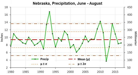
The purpose of this study was to develop a classification scheme that is reliable in most growing season wetness regimes. Recent wet, normal, and dry growing seasons in the COHYST region were identified using the National Oceanic and Atmospheric Administration (NOAA)—National Climatic Data Center (NCDC) climate monitoring portal (http://www.ncdc.noaa.gov/cag/). The time series of the regional average precipitation of June, July, and August from 1980 to 2017 was plotted (Figure 3) along with the long term average of 1901–2000 (239.3 mm), the one and two standard deviations about the mean. From the time series, 2015 was a normal growing season of 276.6 mm of rainfall, and 2012 was a dry year of 95 mm of rainfall during the growing season. The most recent wettest growing season with groundtruth data was 2010 (362.7 mm), closely followed by 2014 (346.7 mm) (Figure 3). Both the 2010 and 2014 growing season rainfall were more than two standard deviations from the long term mean precipitation. For the derivation and calibration of the scheme, 2014 was selected as the wettest season over 2010, because, Landsat 8 imagery available for 2014 was of higher quality than Landsat 7 and 5 imagery available for 2010. In addition, the 2014 growing season had more sampled irrigated (464) and non-irrigated (355) fields than the 2010 growing season. A total of 213 irrigated fields and 280 non-irrigated fields across the region (Figure 2) were used for the development and calibration of the classification scheme. The remaining 142 (irrigated) and 184 (non-irrigated) fields were used for the validation of the classification scheme.
2.4. Normal Difference Vegetation Index and Green Index
NDVI and GI indices were computed from the top of the atmosphere (TOA) reflectance of green, red and near infrared spectral bands as shown below:
where ρgreen, ρred and ρnir are TOA reflectance from band 2, band 3, and band 4, respectively, of Landsat 5 and 7, and band 3, band 4, and band 5, respectively, of Landsat 8. NDVI has been widely used as an important vegetation and irrigation monitoring tool [8,11,12,20,21,22]. GI on the other hand, has been a less exploited vegetation index, yet studies [23,24] have found the index more sensitive to chlorophyll than NDVI, Enhanced Vegetation Index (EVI) [25], and Wide Dynamic Range Vegetation Index (WDRVI) [26].
The high sensitivity of GI is due to the green leaves high absorption (more than 80%) in the green spectrum (e.g., [27,28,29]), and a much lower penetration (four to six times) of blue and red spectrum in the leaf canopy (e.g., [30]). Therefore, in the green spectrum, the absorption of light is adequately high to generate a highly sensitive GI to chlorophyll content but the absorption is much lower in blue and red spectrum, thus preventing index saturation [13,27].
2.5. Surface Energy Balance System (SEBS)
SEBS [15] is a physical model that uses the principle of conservation of energy (Equation (3)) to partition net available energy from the sun, net radiation (Rn), into the major surface energy components; soil heat (G), sensible heat (H) and latent heat (λE) flux.
Rn = λE + H + G
Net radiation (Wm−2) was calculated as the radiation balance of net shortwave and net long wave radiation [31,32,33]. Soil heat flux (Wm−2) was estimated as a fraction of net radiation by an empirical function derived by Choudhury et al. [34], and the constants calibrated by Monteith [35] and Kustas et al. [36]. Sensible heat flux (Wm−2) was estimated by using the similarity theory and solving a system of non-linear equations using the Broyden method [37]. The non-linear equations are the similarity relationships for the profiles of friction velocity, Monin Obukhuv length, aerodynamic resistance, and mean temperature (i.e., the difference between surface temperature and air temperature). The procedure to derive sensible heat flux is methodically described in [15] and requires only wind speed, temperature at a reference height and surface temperature as inputs.
SEBS estimates latent heat flux (evapotranspiration) by interpolating the relative evaporation between the dry-limit and wet-limit [15]. Under the dry-limit, latent heat flux becomes zero due to the limitation of soil moisture, and sensible heat flux is assumed to be at maxima. Under the wet-limit, latent heat flux is at potential rate limited only by the available energy under the given surface and atmospheric conditions, and sensible heat flux is assumed to be at minima. The SEBS evaporative fraction (ETRF) used to derive the irrigation classification index in this study was estimated using Equation (4). SEBS estimates ETRF in the range of 0 to 1 [15]. The normalization of λE by Rn − G serves to reduce the impact of drivers of the evaporative flux that are less directly related to soil moisture stress (e.g., insolation load and atmospheric demand), [38].
The SEBS model inputs are surface emissivity, albedo, surface temperature, and NDVI. These inputs were processed from spectral reflectance and radiance of Landsat optical and thermal bands. The other inputs include weather station variables, air temperature, air pressure, relative humidity, wind speed, wind speed and measurement height, and day-of-year and time of (Landsat) overpass.
2.6. Irrigation Indices Development
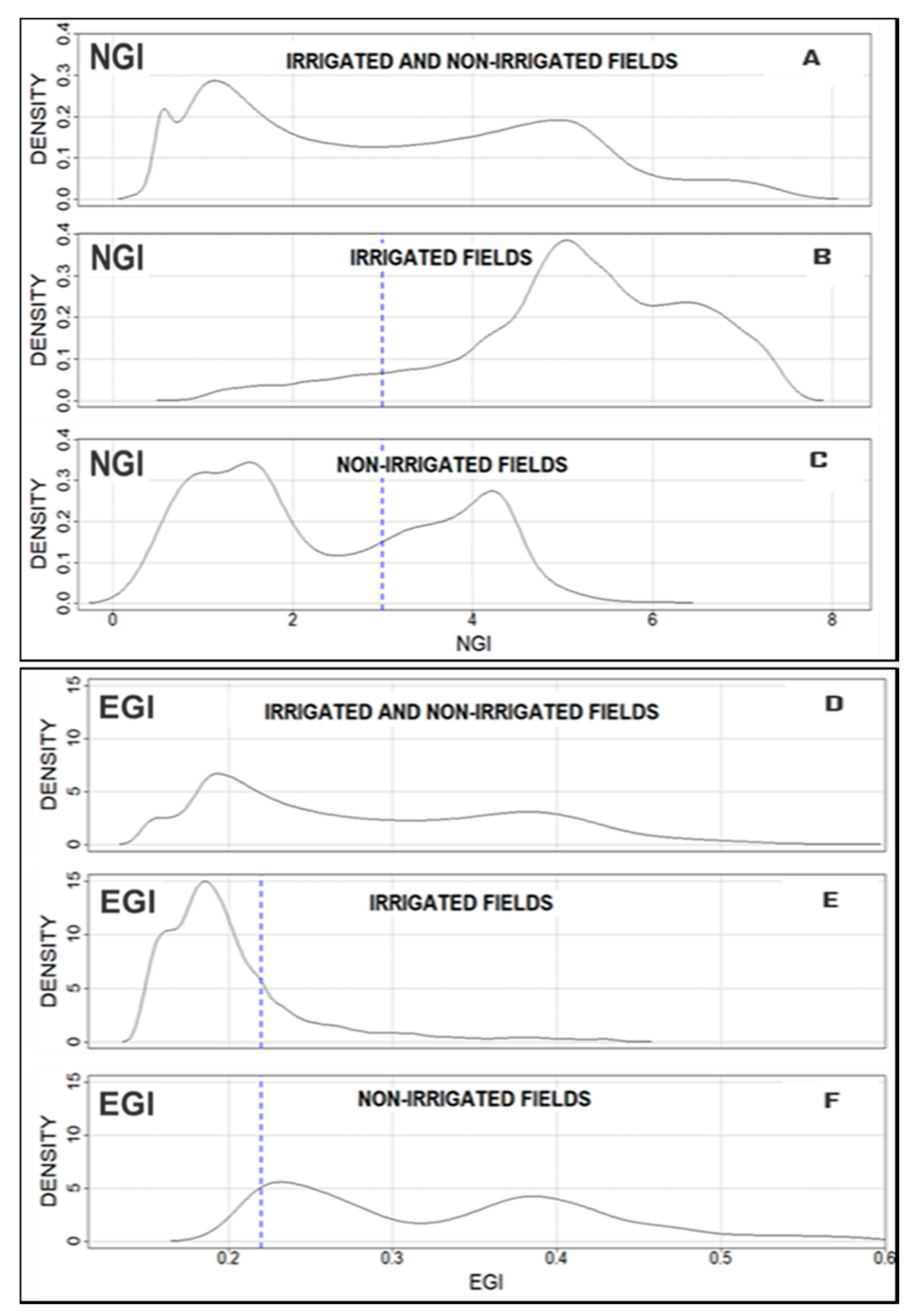
Several discrete and compound indices derived from NDVI, EVI, GI, maximum NDVI and GI, cumulative NDVI and EVI, ETRF, max daily λE, and cumulative daily λE were evaluated for the most effective classifiers of irrigation croplands in the region. Preceding, non-agricultural areas such as cities, forests, conservation ecological areas, and water features were masked from the indices using CDL data from the 2014 growing season. Using groundtruth data from the 2014 growing season, irrigated and non-irrigated pixels of an index were extracted, and distribution functions were then fit on the irrigated pixels, non-irrigated pixels, and all pixels combined as shown in Figure 4. Most indices derived formed an empirical bimodal distribution (as shown in Figure 4A,D) on a mixture of irrigated and non-irrigated croplands, however the indices produced different thickness in the middle section of the distribution. In the wet season, the middle section is much thicker, since the vegetation cover of irrigated and non-irrigated croplands is insignificantly different. During the dry season or arid climate, the middle section is, as expected, thin, since the vegetation cover of non-irrigated and irrigated cropland is usually significantly different.
An ideal index in this study was expected to generate a bimodal distribution function that accurately separated irrigated and non-irrigated pixels to the either side of the bimodal during the growing season. Two compound indices EGI (Equation (5)) and NGI (Equation (6)) derived from ETRF, GI, and NDVI were found to generate the widest distribution contrast between irrigated and non-irrigated conditions in 2014, and were ultimately selected for the classification scheme.
Figure 4A shows the bimodal distribution of NGI for both irrigated and non-irrigated pixels combined. The NGI distribution function isolated irrigated pixels to the right with a long tail to the left (Figure 4B). The NGI distribution function isolated most of the non-irrigated pixels to the left, with a bimodal function and short tail to the right. By comparing the x-axes of Figure 4B,C, it is important to notice that most of non-irrigated pixels were isolated to the long tail section of the irrigated distribution. Similarly, Figure 4D shows the bimodal distribution of EGI for both irrigated and non-irrigated pixels combined. However, in a reverse fashion, this distribution isolated irrigated pixels to the left and non-irrigated to the right (Figure 4E,F).
2.7. Thresholding
Although the two indices had the most accentuated contrast between irrigated and non-irrigated pixels, there was still some overlap of irrigated and non-irrigated pixels in the middle of the distributions. For NGI distribution, most of the irrigated pixels had values of greater than 4 (Figure 4B), and most non-irrigated pixels had values of less than 5 (Figure 4C), with significant overlap between index values 2 and 5, which is the mid-section of the bimodal distribution (Figure 4C). For EGI distribution, most of the irrigated pixels had values of less than 0.25 (Figure 4E), and most non-irrigated pixels had values of greater than 0.20 (Figure 4F), with significant overlap between index values 0.2 and 0.28. Therefore, to enhance the classification of irrigated pixels, the two indices were synergized to take advantage of their distribution properties of contrasting irrigation from non-irrigation status.
The synergy of the two indices was formulated by first applying a preliminary loose threshold of value 3 on NGI to exclude non-irrigated pixels (NGI < 3) (Figure 4C), then eliminating the remaining non-irrigated pixels in NGI conditioned on a tight EGI threshold value of 0.22 (EGI > 0.22) (Figure 4F). The two thresholds (NGI = 3 and EGI = 0.22) were calibrated by iterating in the middle of the bimodal distribution, where the irrigated and non-irrigated pixels overlapped, using a computer program (in Python) until the combination of the two thresholds accurately classified all irrigated and non-irrigated fields in the groundtruth data. Figure 5 show the distribution of NGI for irrigated (Figure 5A) and non-irrigated (Figure 5B) pixels after the calibrated thresholds were applied to all fields in the region.
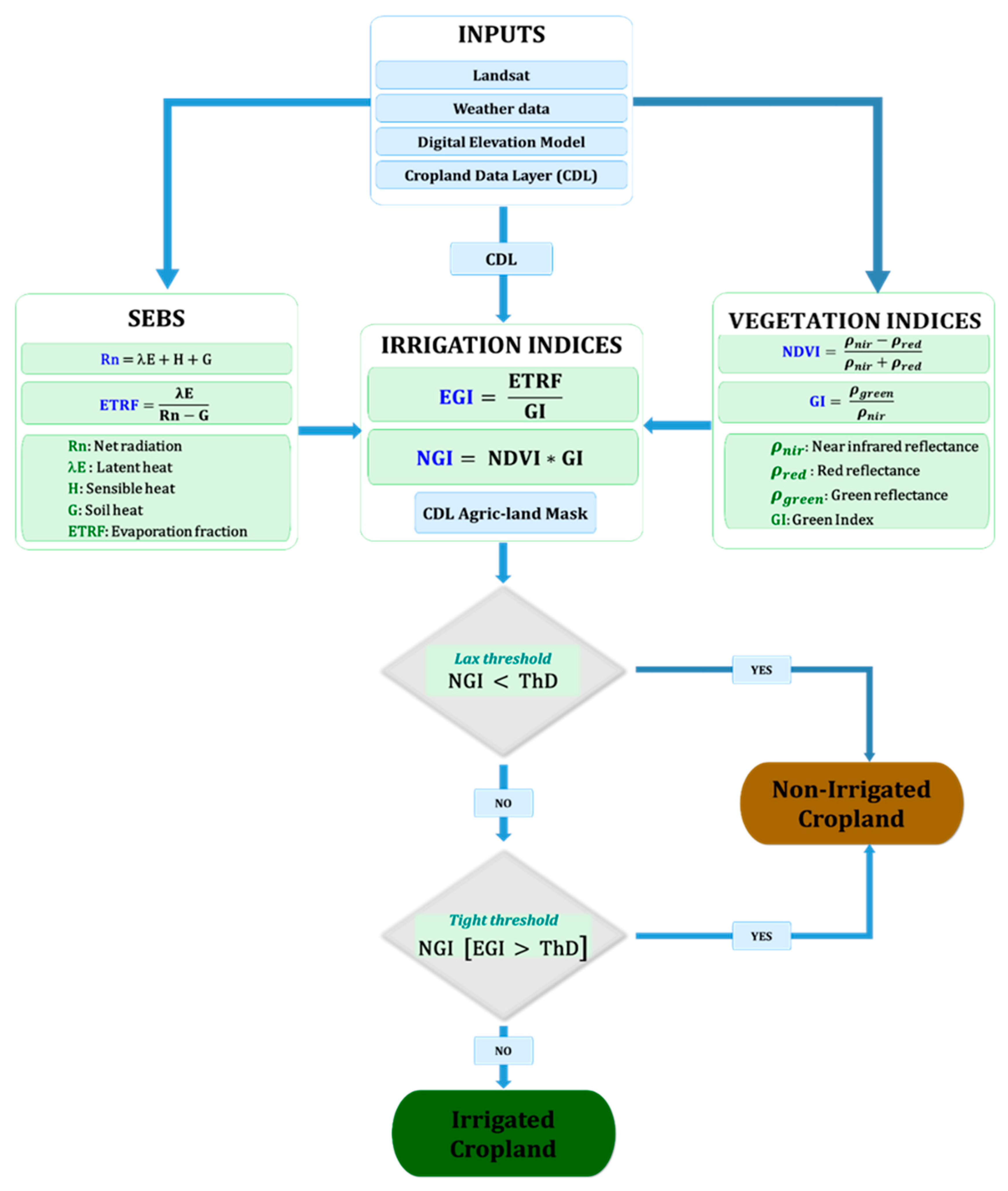
A conceptual flow diagram (Figure 6) describes the implementation of the scheme, including the data inputs, derivation of the indices, and thresholding of indices. Methodically, ETRF from SEBS, NDVI, and GI, are derived separately, and are formulated into EGI and NGI. A crop mask from CDL for the growing season is applied on the two indices to remove non-agricultural areas. The NGI as the based index, is thresholded first to remove non-irrigated pixels. The remaining non-irrigated pixels in NGI are then removed conditioned on EGI threshold. As shown in Figure 6, the non-irrigated pixels from the two thresholdings are combined to form the non-irrigated fields. The entirety of the scheme in Figure 6 is also referred to hereafter as the NDVI-Evaporation Fraction-Green Index (NEG) classification scheme.
2.8. Performance Assessment
The derived classification scheme was validated and evaluated on the growing seasons of 2010, 2014, and 2015, which had groundtruth data on irrigation status in the COHYST region. The performance of the classification scheme was evaluated using Kappa analysis, confusion (error) matrix referenced to groundtruth data, the coefficient of determination (R2) as a measure of goodness of fit (i.e., the measure of variance in NASS county data accounted for by NEG county aggregated estimates), Root Mean Square Deviation (RMSD) as a measure of the absolute difference between NASS and NEG, and Mean Absolute Percent Error (MAPE) as a measure of NEG accuracy in percentage terms (Equation (7)). Where N is the number of counties. Note, the counties partitioned by the COHYST boundary were excluded from the NASS-NEG county performance assessment.
3. Results
3.1. NEG Classification Scheme and Groundtruth
The NEG classification scheme was validated on groundtruth data available from the growing seasons of 2010, 2014, and 2015. The results from the error matrix analysis in reference to groundtruth for the three years area are presented in Table 1. In 2015, a normal year of precipitation during the growing season, 93% (i.e., 567 of 611) of NEG irrigated fields and 86% (i.e., 1402 of 1635) of non-irrigated fields matched groundtruth data. In 2014, a wet year, the scheme had a performance of 98% (i.e., 453 of 464) of NEG irrigation fields and 83% (i.e., 294 of 355) of non-irrigated fields matching groundtruth data. In 2010, also a wet year during the growing season, 90% (i.e., 704 of 782) of NEG irrigated fields and 81% (i.e., 260 of 321) of non-irrigated fields matched groundtruth data. The overall accuracy of classifying irrigation for the three years combined was 92.1%. The lower producer accuracy for the non-irrigated croplands in Table 1 was due to some of the non-irrigated groundtruth locations being sampled from the corners of the center pivots. If these points were within 60 m from the pivot circle line, they were sometimes misclassified as irrigated.
3.2. Spatial Distribution of Irrigation
There is a characteristic distribution of extensive irrigation in the east that disperses westward of the region (Figure 7). York and Hamilton counties, both in the east, were the most irrigated counties with more than 70% of county area classified as irrigated cropland. In the northwest of the region a few scattered fields were classified as irrigated. The most irrigated crop in the northwest was alfalfa; for instance, in Arthur and Garden counties, 58.3% and 60.6% of irrigated cropland was alfalfa during the 2015 growing season. In McPherson County, however, pasture was the most irrigated crop at 42%. Across the region, a total of 1,606,008 ha in 2015 and 1,462,004 ha in 2010 were classified as irrigated, many of which were corn and soybean.
It is evident that the extent and intensity of irrigation in a region depends on four key factors: rainfall, water accessibility, topography, and soil type. The northwest, as part of the Nebraska Sandhills, is mostly sandy and semi-arid. During the three months (June, July, and August) of intensive irrigation in the region, rainfall distribution across the region decreases from east to west by 89 mm (239 to 328 mm), Figure 8. The difference is significant given that the average seasonal evapotranspiration for irrigated corn is 548 mm and 452 mm for soybean [39]. Precipitation may be a constraining factor, however, the main limiting factor of intensive irrigation expansion in the west is the nutrient-deficient and low water holding capacity sandy soils that dominate the region. Consequentially, the region is dominated by grass and pasture for ranching, winter wheat, and alfalfa. Nonetheless, close to the river basin in Keith, Perkins, and Lincoln counties, irrigation of major crops such as corn and soybeans is widespread. The spatial distribution contrast in the intensity of irrigation between the east and west of the region means that there is a higher groundwater and surface water consumption in the east than in the west.
By far, the most grown and irrigated crops across the region were corn and soybean (Figure 7A,B). Sixty eight percent (68%) of the region in 2015 was irrigated corn and 28% was irrigation soybean. In 2010, 67% of the region was irrigated corn and about 31% was irrigation soybean (Table 2). Note that, because the classification scheme was applied during the intensive irrigation months of July and August, irrigated winter wheat, which is typically harvested from late June, may be fittingly classified as non-irrigated or as other short season crops. Therefore, despite winter wheat being a major crop in the region, the further classification of irrigated croplands into crop-types excluded winter wheat.
3.3. NEG Classification Scheme and NASS Statistics
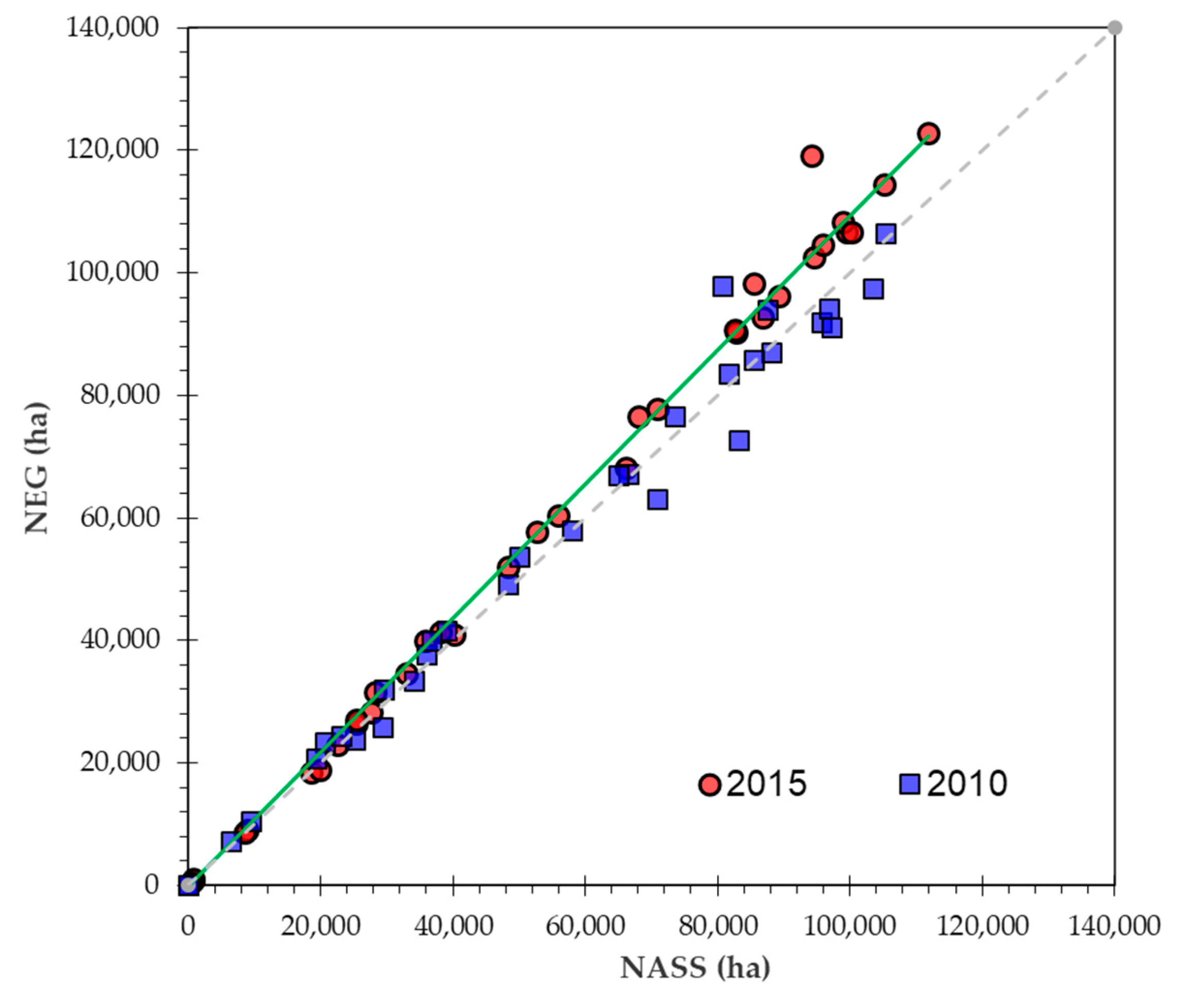
As the official estimates of national agricultural statistics, NASS county irrigated acreages were used as cross reference, rather than measures of accuracy, to assess the performance of NEG classification scheme at the county aggregated level. The regression results (R2) showed that NEG county aggregates explained 98% and 99% variation in NASS county data (Table 3, Figure 9) for the 2010 and 2015 growing seasons, respectively. The MAPE statistics had comparable overestimation values of 6.3% to 7.48% for the two growing seasons (Table 3). The overestimation is probable since NASS statistics are compiled from the top most grown crops in the region; corn, soybean, Alfalfa, etc. The irrigation acreages of other crops such as sorghum, small grains, potatoes, among others, are assumed to be negligible.
4. Discussion
4.1. Dual Indices and Single Index
Single-index schemes have been successfully used by several studies (e.g., [10,41,42]) to classify irrigated croplands. Peak NDVI and differential NDVI have been the most commonly studied indices to classify irrigated croplands [11,43,44]. These methods, however, may be subject to misclassification due to NDVI saturation [45], disparity in crop development as a result of crop management practices, such as planting dates and cultivar varieties. Indeed, the anthropogenic involvement in land use patterns increases the difficulty of classifying crop water management practices (irrigation and non-irrigated) as opposed to classifying land cover patterns. For a successful classification of land use patterns such as irrigation status, knowledge of crop- and land-management, or some understanding of when and where farmers plant, fertilize and supply of other supplements to enhance crop development is essential [5].
Pervez and Brown [10] considered peak NDVI as a proxy for the peak level of photosynthetic activity and biomass. And at the peak NDVI, irrigated and non-irrigated crops exhibited the highest NDVI differential. However, the effectiveness of peak NDVI differential is constrained by index saturation and sensitivity to crop variety. Indeed, it is only possible to classify irrigation using a single index as long as the area contains only a few crop types [5]. And, in the case of wet growing seasons, the peak NDVI differential is marginal for successful irrigation classification.
The synergy of two functionally different indices presented in this study increases the classification proficiency by adding another classifying layer which re-characterizes misclassified croplands by the base index. The two NEG indices are functionally different because NGI is purely a phenological index, and EGI is both a phenological and soil water stress index. Therefore, for EGI, in addition to classifying irrigation based on long term cumulative vegetation development difference as NGI, also classifies irrigation based on short term soil water stress difference between irrigated and non-irrigated crops. The short term ability based on soil water stress enhances the implementation of NEG scheme in humid climate and wet growing seasons.
A dynamic thresholding scheme derived by Wardlow and Egbert [7] calibrated NDVI thresholds on NASS statistics to estimate county irrigation acreages. The results correlated with NASS estimates, but the thresholds required calibration for every county and different growing season, thus subjecting the scheme to the availability and accuracy of NASS statistics. Our results show that NEG classification scheme was not only viable for wet and normal growing seasons, but also that the fixed thresholds were reliable across the different counties in the region. Despite the viability of NEG classification scheme across wide climate variability and seasonal variability, more validation is necessary to evaluate the suitability of the scheme in distinctively different agro-climate regions. A number of factors can potentially impact the performance of NEG classification scheme in agro-climate regions that are different from the COHYST region. Besides, the COHYST region is dominated by two crops (corn and soybean); therefore, increase in crop variability in a different region may impact the classification performance. Furthermore, the crops in the COHYST region are typically narrow row crops, thus NEG performance may also differ in wide row crops such as vineyards and orchards.
4.2. Seasonal Development of NGI and EGI
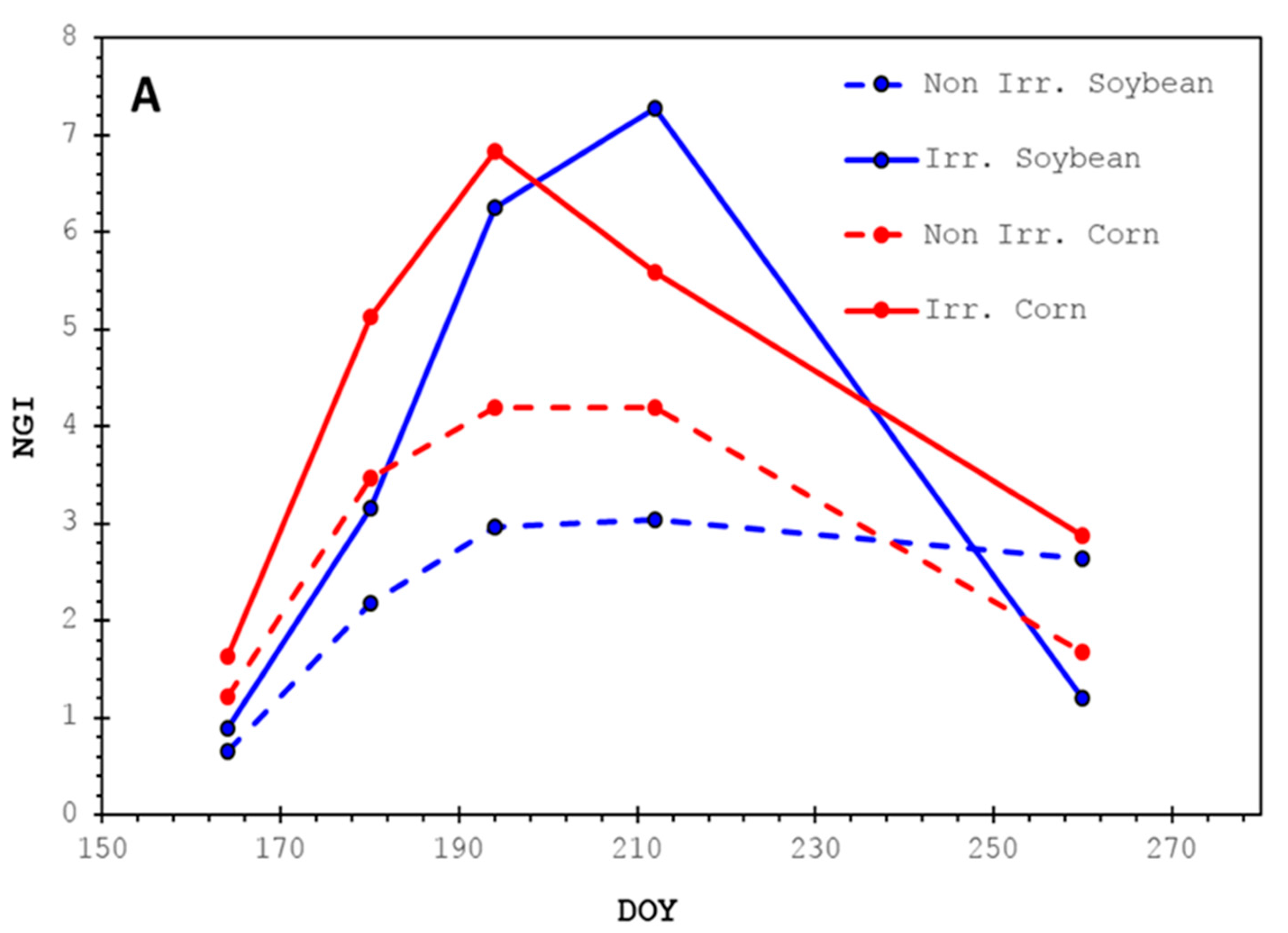
The development of NGI during the growing season shows that during the initial growth stage, the index values for irrigated and non-irrigated corn and soybean were nearly comparable (Figure 10A). In the study region, evapotranspiration during the initial growth stage is primarily soil evaporation [46] driven by soil moisture from the previous winter snow melt and spring rains. As the crop matures, the NGI of irrigated and non-irrigated crops diverged owing to soil moisture availability. The cumulative vegetation growth differential peaks during the mid-season of crop development, and depreciates during late-season as the crop undergoes senescence. In addition, non-irrigated crops have a reduced growth rate relative to irrigated crops which further augment the vegetative growth differential during the mid-season crop stage. Therefore, during the mid-season of crop development, NGI was highly different for the two crop water management practices for both corn and soybean (Figure 10A). The peak NGI value for irrigated corn was about 7, while non-irrigated corn only reached a peak of about 4. The growth sensitivity coefficient, calculated as the difference between of mid-stage (highest) value and initial value of irrigated crop divided by the difference between mid-stage (highest) value and initial value of non-irrigated crop, for corn and soybean was 1.75 and 2.70, respectively, during the mid-season of crop development. The EGI growth sensitivity coefficient between irrigated and non-irrigated was about 1.0 for both crops (Figure 10B). Likewise, EGI had a higher difference between irrigated and non-irrigated soybean than corn during the mid-season stage. Since both indices generated maximum contrast between irrigated and non-irrigated conditions during mid-season stage, for optimal classification results, the classification scheme was (and should in principle be) implemented during the mid-season of crop development (which normally lasts between mid-July and mid-August in the COHYST region).
4.3. Application in Humid to Arid Climate Regimes, and Wet to Dry Growing Seasons
Irrigation application in wet and semi-wet climate regions or during wet growing seasons is a supplementary crop water management practice. In these agro-climate and seasonal scenarios, the vegetation canopy of non-irrigated crops is usually insignificantly different from irrigated crops, though the yield may differ at the end of the growing season [47]. For that reason, irrigation classification is essentially an arduous procedure since the phenological difference in vegetation canopy is subtle for classification schemes to reliably detect the spectral difference between irrigated and non-irrigated surfaces. Several studies (e.g., [10,12,21]) have determined that the most widely used classification schemes are based on vegetation indices that are only spectrally sensitive to phenological variation under severe conditions such as droughts or desert climate. In this study, the proposed dual index scheme assimilates ETRF (scaled by GI), a phenological and soil water stress index [48] that is sensitive to short and long term water sufficiency or deficiency. Therefore, the cumulative vegetative difference due to long term water availability is the principal factor for detecting irrigated surfaces from a non-irrigated in humid climate and wet growing seasons. Such conditions took effect in the eastern part of COYHST region in 2014 and 2010; that is, a humid agro-climate region in a wet growing season. Since EGI is a proxy soil water stress index, prioritizing Landsat images that are available after a long period without rainfall is an important caveat in the NEG classification scheme to enhance irrigation classification in a wet seasons or climate regions.
In arid climate and dry growing seasons, irrigated and non-irrigated cropland distinction is a clear-cut classification due to wide spectral difference between the two surfaces, and likely crop failure for non-irrigated croplands [10]. Dry conditions render leaf cells to shrink, consequently shriveling or rolling the leaves of the canopy. Concomitant with the structural change of the canopy is the reduced production of chlorophyll. These changes, phenology and bioprocesses, result in less scattering in near infrared and less absorption of visible red light [49]. Thus far, none of the years (2010, 2014, and 2015) considered and with groundtruth data, were dry years in the region. Therefore, to evaluate the performance of the NEG classification scheme in a dry year, the scheme was implemented on the 2012 growing season, and on a smaller area of twelve counties in the middle of COYHST region and wrapped in two adjacent Landsat scenes (P30/R32 and P29/R32). The 2012 growing season was an extraordinary drought in intensity and extent across the United States. During the growing season, the U.S. Department of Agriculture declared 1692 counties, about 63% of the conterminous United States, as disaster areas [50]. Without groundtruth the performance of NEG scheme was only evaluated with respect to NASS irrigation statistics, and the performance was comparable to other years with R2 of 97% and MAPE of 8.49%. The semi-arid western part of the region in a dry year and the humid eastern part of the region in a wet year were considered in this study as the two extremes of a climate spectrum in which many other regional climate patterns fall in between, and in which NEG scheme is inferred to perform capably.
5. Conclusions
An irrigation classification scheme applicable across a wide range of regional climates and inter-growing seasonal precipitation is derived from the SEB partitioning and vegetation indices, and calibrated on the wettest growing season. The scheme is a synergy of two indices, NGI and EGI, with distribution functions that highly contrast irrigated and non-irrigated croplands. The two indices are functionally different because NGI is a phenological index and EGI is both a phenological and soil water stress index. For optimal classification, the scheme should, in principle, be implemented on satellite imagery acquired after a long dry period without precipitation and during mid-season stage of crop growth. The scheme was applied to a region with wide climate variation and to multiple growing seasons. The results revealed that across multiple growing seasons, the classification scheme was 92.1% accurate and explained 97% variation in NASS county irrigation statistics. Although further tests would be valuable, the performance demonstrates that NEG irrigation classification scheme is an accurate and consistent approach to classify and estimate irrigated acreage across a wide range of regional climates, and during dry, normal and wet growing seasons.
Acknowledgments
This research project was carried out with funding provided by State of Nebraska Department of Natural Resources (DNR Contract #807). We also acknowledge Riverside Technology, Inc., for collecting the Irrigation groundtruth data used in this project. The following DNR staffs are also thanked for their support in the completion of this study project: Amy Zoller and Zablon Adane.
Author Contributions
M.P., D.M., and R.L. designed research; M.P., D.M., and R.L. performed research; D.M. contributed analytic tools; M.P., D.M., and R.L. analyzed data; and M.P., D.M., and R.L. wrote the paper
Conflicts of Interest
The authors declare no conflict of interest.
Appendix A

Table A1.
Landsat scene identification (ID), acquisition spacecraft and date, and path and row of images used for the project.
Table A1.
Landsat scene identification (ID), acquisition spacecraft and date, and path and row of images used for the project.
| SCENE ID | SPACECRAFT ID | DATE | PATH | ROW |
|---|---|---|---|---|
| LE70310312010207EDC00 | Landsat 7 | 26 July 10 | 31 | 31 |
| LE70310312010239EDC00 | Landsat 7 | 27 July 10 | 31 | 31 |
| LE70310322010207EDC00 | Landsat 7 | 26 July 10 | 31 | 32 |
| LE70310322010239EDC00 | Landsat 7 | 27 July 10 | 31 | 32 |
| LT50310322010247EDC00 | Landsat 5 | 04 Sept 10 | 31 | 32 |
| LE70320312010230EDC00 | Landsat 7 | 18 Aug 10 | 32 | 31 |
| LT50320312010222PAC01 | Landsat 5 | 10 Aug 10 | 32 | 31 |
| LE70320312010246EDC00 | Landsat 7 | 03 Sept 10 | 32 | 31 |
| LE70320322010198EDC00 | Landsat 7 | 17 July 10 | 32 | 32 |
| LT50320322010222PAC01 | Landsat 5 | 10 Aug 10 | 32 | 32 |
| LE70320322010246EDC00 | Landsat 7 | 03 Sept 10 | 32 | 32 |
| LT50290312010217EDC00 | Landsat 7 | 05 Aug 10 | 29 | 31 |
| LT50290312010233EDC00 | Landsat 5 | 21 Aug 10 | 29 | 31 |
| LE70290322010177EDC00 | Landsat 7 | 26 June 10 | 29 | 32 |
| LT50290322010233EDC00 | Landsat 5 | 21 Aug 10 | 29 | 32 |
| LT50300312010208PAC01 | Landsat 5 | 27 July 10 | 30 | 31 |
| LT50300312010176EDC00 | Landsat 5 | 25 June 10 | 30 | 31 |
| LT50300322010208PAC01 | Landsat 5 | 27 July 10 | 30 | 32 |
| LT50300322010192EDC00 | Landsat 5 | 11 July 10 | 30 | 32 |
| LC80290312015199LGN00 | Landsat 8 | 18 July 15 | 29 | 31 |
| LE70290312015223EDC00 | Landsat 7 | 11 Aug 15 | 29 | 31 |
| LE70290312015255EDC00 | Landsat 7 | 12 Sept 15 | 29 | 31 |
| LC80290322015199LGN00 | Landsat 8 | 18 July 15 | 29 | 32 |
| LC80290322015215LGN00 | Landsat 8 | 03 Aug 15 | 29 | 32 |
| LE70300312015198EDC00 | Landsat 7 | 17 July 15 | 30 | 31 |
| LE70300312015214EDC00 | Landsat 7 | 02 Aug 15 | 30 | 31 |
| LC80300312015238LGN00 | Landsat 8 | 26 Aug 15 | 30 | 31 |
| LE70300322015198EDC00 | Landsat 7 | 17 July 15 | 30 | 32 |
| LE70300322015214EDC00 | Landsat 7 | 02 Aug 15 | 30 | 32 |
| LC80300322015238LGN00 | Landsat 8 | 26 Aug 15 | 30 | 32 |
| LC80310312015197LGN00 | Landsat 8 | 16 July 15 | 31 | 31 |
| LC80310312015245LGN00 | Landsat 8 | 02 Sept 15 | 31 | 31 |
| LC80310322015197LGN00 | Landsat 8 | 16 July 15 | 31 | 32 |
| LC80310322015213LGN00 | Landsat 8 | 01 Aug 15 | 31 | 32 |
| LC80310322015245LGN00 | Landsat 8 | 02 Sept 15 | 31 | 32 |
| LC80320312015204LGN00 | Landsat 8 | 23 July 15 | 32 | 31 |
| LC80320312015236LGN00 | Landsat 8 | 24 Aug 15 | 32 | 31 |
| LC80320322015204LGN00 | Landsat 8 | 23 July 15 | 32 | 32 |
| LC80320322015236LGN00 | Landsat 8 | 24 Aug 15 | 32 | 32 |
References
- Morrison, J.; Morikawa, M.; Murphy, M.; Schulte, P. Water Scarcity and Climate Change: Growing Risks for Businesses and Investors; A Ceres Report; Pacific Institute: Oakland, CA, USA, 2009. [Google Scholar]
- Ibrahim, A.M. The Nile Basin Cooperative Framework Agreement: The Beginning of the End of Egyptian Hydro-Political Hegemony. Mo. Environ. Law Policy Rev. 2011, 18. Available online: http://scholarship.law.missouri.edu/cgi/viewcontent.cgi?article=1395&context=jesl (accessed on 28 November 2017). [CrossRef]
- Nebraska Department of Natural Resources (NDNR). Annual Report and Plan of Work for the Nebraska State Water Planning and Review Process. Nebraska Department of Natural Resources. 15 September 2007. Available online: http://govdocs.nebraska.gov/epubs/N1500/A004-2007.pdf (accessed on 28 November 2017).
- Aiken, J.D. The Republican River: Negotiation, arbitration, and a federal water master. Cornhusker Econ. 2008, 382. Available online: http://digitalcommons.unl.edu/agecon_cornhusker/382/.
- Ozdogan, M.; Yang, Y.; Allez, G.; Cervantes, C. Remote sensing of irrigated agriculture: Opportunities and challenges. Remote Sens. 2010, 2, 2274–2304. [Google Scholar] [CrossRef]
- Alexandris, T.K.; Zalidis, G.C.; Silleos, N.G. Mapping irrigated area in Mediterranean basins using low cost satellite Earth Observation. Comput. Electr. Agric. 2008, 64, 93–103. [Google Scholar] [CrossRef]
- Wardlow, B.D.; Egbert, S.L. Large-area crop mapping using time-series MODIS 250 m NDVI data: An assessment for the U.S. Central Great Plains. Remote Sens. Environ. 2008, 112, 1096–1116. [Google Scholar] [CrossRef]
- Jin, N.; Ren, W.; Feng, M.; Sun, R.; He, L.; Zhuang, W.; Yu, Q. Mapping Irrigated and Rainfed Wheat Areas Using Multi-Temporal Satellite Data. Remote Sens. 2016, 8, 207. [Google Scholar] [CrossRef]
- Ambika, A.K.; Wardlow, B.; Mishra, V. Remotely sensed high resolution irrigated area mapping in India for 2000 to 2015. Sci. Data 2016, 3, 160118. [Google Scholar] [CrossRef] [PubMed]
- Pervez, M.S.; Brown, J.F. Mapping irrigated lands at 250-m scale by merging MODIS data and national agricultural statistics. Remote Sens. 2010, 2, 2388–2412. [Google Scholar] [CrossRef]
- Pervez, S.M.; Budde, M.; Rowland, J. Mapping irrigated areas in Afghanistan over the past decade using MODIS NDVI. Remote Sens. Environ. 2014, 149, 155–165. [Google Scholar] [CrossRef]
- Brown, J.F.; Pervez, M.S. Merging remote sensing data and national agricultural statistics to model change in irrigated agriculture. Agric. Syst. 2014, 127. [Google Scholar] [CrossRef]
- Gitelson, A.A.; Gritz, U.; Merzlyak, M.N. Relationships between leaf chlorophyll content and spectral reflectance and algorithms for non-destructive chlorophyll assessment in higher plant leaves. J. Plant Physiol. 2003, 160, 271–282. [Google Scholar] [CrossRef] [PubMed]
- Gitelson, A.A.; Vina, A.; Ciganda, V.; Rundquist, D.C.; Arkebauer, T.J. Remote estimation of canopy chlorophyll content in crops. Geophys. Res. Lett. 2005, 32, L08403. [Google Scholar] [CrossRef]
- Su, Z. The surface energy balance system (SEBS) for estimation of turbulent heat fluxes. Hydrol. Earth Syst. Sci. 2002, 6, 85–99. [Google Scholar] [CrossRef]
- Dappen, P.; Merchant, J.; Ratcliffe, I.; Robbins, C. Delineation of 2005 Land Use Patterns for the State of Nebraska Department of Natural Resources; Final Report; Center for Advanced Land Management Information Technologies (CALMIT): Lincoln, NE, USA, 2007. [Google Scholar]
- Szilagyi, J.; Jozsa, J. MODIS-Aided Statewide Net Groundwater-Recharge Estimation in Nebraska. Ground Water 2013, 51, 735–744. [Google Scholar] [CrossRef] [PubMed]
- Han, W.; Yang, Z.; Di, L.; Mueller, R. CropScape: A Web service based application for exploring and disseminating US conterminous geospatial cropland data products for decision support. Comput. Electron. Agric. 2012, 84, 111–123. [Google Scholar] [CrossRef]
- Riverside Technology, Inc. 2014 COHYST Ground Truth Data Collection for Use in Landcover Classification Task 1: Image Processing and Ground Truth Data Collection; Report; Cooperative Hydrology Study (COHYST): Lincoln, NE, USA, 2015. [Google Scholar]
- Goward, S.N.; Markham, B.; Dye, D.; Dulaney, W.; Yang, J. Normalized difference vegetation index measurements from the Advanced Very High Resolution Radiometer. Remote Sens. Environ. 1991, 35, 257–277. [Google Scholar] [CrossRef]
- DeFries, R.S.; Hansen, M.; Townshend, J.R.G.; Sohlberg, R. Global land cover classifications at 8 km spatial resolution: The use of training data derived from Landsat imagery in decision tree classifiers. Int. J. Remote Sens. 1998, 19, 3141–3168. [Google Scholar] [CrossRef]
- Mutiibwa, D.; Irmak, S. Estimation of crop coefficients from AVHRR-based NDVI for analyzing long-term trends in evapotranspiration in relation to changing climate in the USA High Plains. Water Resour. Res. 2012, 49, 231–244. [Google Scholar] [CrossRef]
- Ozdogan, M.; Gutman, G. A new methodology to map irrigated areas using multi-temporal MODIS and ancillary data: An application example in the continental US. Remote Sens. Environ. 2008, 112, 3520–3537. [Google Scholar] [CrossRef]
- Gitelson, A.A.; Viña, A.; Masek, J.G.; Verma, S.B.; Suyker, A.E. Synoptic monitoring of gross primary productivity of maize using Landsat data. IEEE Geosci. Remote Sens. Lett. 2008, 5, 2. [Google Scholar] [CrossRef]
- Huete, A.R.; Justice, C.O.; van Leeuwen, W.J.D. MODIS Vegetation Index, Algorithm Theoretical Basis Document. 30 April 1999; NASA Goddard Space Flight Centre: Greenbelt, MD, USA. Available online: http://gis-lab.info/docs/atbd_mod13.pdf (accessed on 28 November 2017).
- Gitelson, A.A. Wide dynamic range vegetation index for remote quantification of biophysical characteristics of vegetation. J. Plant Physiol. 2004, 161, 165–173. [Google Scholar] [CrossRef] [PubMed]
- Thomas, J.R.; Gaussman, H.W. Leaf reflectance vs. leaf chlorophyll and carotenoid concentration for eight crops. Agron. J. 1977, 69, 799–802. [Google Scholar] [CrossRef]
- Buschmann, C.; Nagel, E. In vivo spectroscopy and internal optics of leaves as basis for remote sensing of vegetation. Int. J. Remote Sens. 1993, 14, 711–722. [Google Scholar] [CrossRef]
- Gitelson, A.A.; Merzlyak, M.N. Quantitative estimation of chlorophyll a using reflectance spectra: Experiments with autumn chestnut and maple leaves. J. Photochem. Photobiol. B 1994, 22, 247–252. [Google Scholar] [CrossRef]
- Merzlyak, M.N.; Gitelson, A.A. Why and what for the leaves are yellow in autumn? On the interpretation of optical spectra of senescing leaves (Acer platanoides L.). J. Plant Physiol. 1995, 145, 315–320. [Google Scholar] [CrossRef]
- Su, Z.; Pelgrum, H.; Menenti, M. Aggregation effects of surface heterogeneity in land surface processes. Hydrol. Earth Syst. Sci. 1999, 3, 549–563. [Google Scholar] [CrossRef]
- Su, Z. A Surface Energy Balance System (SEBS) for estimation of turbulent heat fluxes from point to continental scale. In Advanced Earth Observation—Land Surface Climate; Su, Z., Jacobs, C., Eds.; Publications of the National Remote Sensing Board (BCRS): Delft, The Netherlands, 2001; USP-2, 01–02; p. 184. [Google Scholar]
- Samani, Z.; Bawazir, A.S.; Bleiweiss, M.; Skaggs, R.; Tran, V.D. Estimating daily net radiation overvegetation canopy through remote sensing and climatic data. J. Irrig. Drain. Eng. 2007, 133, 291–297. [Google Scholar] [CrossRef]
- Choudhury, B.J.; Idso, S.B.; Reginato, R.J. Analysis of an empirical model for soil heat flux under a growing wheat crop for estimating evaporation by an infrared-temperature based energy balance equation. Agric. For. Meteorol. 1987, 39, 283–297. [Google Scholar] [CrossRef]
- Monteith, J.L. Principles of Environmental Physics; Edward Arnold Press: London, UK, 1973; p. 241. [Google Scholar]
- Kustas, W.P.; Daughtry, C.S.T. Estimation of the soil heat flux/net radiation ratio from spectral data. Agric. For. Meteorol. 1989, 49, 205–223. [Google Scholar] [CrossRef]
- Press, W.H.; Teukolsky, S.A.; Vetterling, W.T.; Flannery, B.P. Numerical Recipes in C: The Art of Scientific Computing; Cambridge University Press: Cambridge, UK, 1997; 994p. [Google Scholar]
- Anderson, M.C.; Zolin, C.; Sentelhas, P.C.; Hain, C.R.; Semmens, K.; Tugrul Yilmaz, M.; Gao, F.; Otkin, J.A.; Tetrault, R. The Evaporative Stress Index as an indicator of agricultural drought in Brazil:an assessment based on crop yield impacts. Remote Sens. Environ. 2016, 174, 82–99. [Google Scholar] [CrossRef]
- Suyker, A.; Verma, B.S. Evapotranspiration of irrigated and rainfed maize–soybean cropping systems. Agric. For. Meteorol. 2009, 149, 443–452. [Google Scholar] [CrossRef]
- Daly, C.; Halbleib, M.; Smith, J.I.; Gibson, W.P.; Doggett, M.K.; Taylor, G.H.; Curtis, J.; Pasteris, P.A. Physiographically-sensitive mapping of temperature and precipitation across the conterminous United States. Int. J. Climatol. 2008, 28, 2031–2064. [Google Scholar] [CrossRef]
- Zhu, X.; Zhu, W.; Zhang, J.; Pan, Y. Mapping irrigated areas in China from remote sensing and statistical data. IEEE J. Sel. Top. Appl. Earth Obs. Remote Sens. 2014, 7, 4490–4504. [Google Scholar] [CrossRef]
- Ozdogan, M.; Salvucci, G.D.; Anderson, B.C. Examination of the Bouchet-Morton complementary relationship using a mesoscale climate model and observations under a progressive irrigation scenario. J. Hydrometeorol. 2006, 7, 235–251. [Google Scholar] [CrossRef]
- Kamthonkiat, D.; Honda, K.; Turral, H.; Tripathi, N.K.; Wuwongse, V. Discrimination of irrigated and rainfed rice in a tropical agricultural system using SPOT VEGETATION NDVI and rainfall data. Int. J. Remote Sens. 2005, 26, 2527–2547. [Google Scholar] [CrossRef]
- Peterson, D.; Whistler, J.; Egbert, S.; Brown, C.J. Mapping irrigated lands by crop type in Kansas. Pecora 18 Proc. 2011. [Google Scholar]
- Huete, A.R.; Didan, K.; Rodriguez, E.P.; Gao, X.; Ferreira, L.G. Overview of the radiometric and biophysical performance of the MODIS vegetation indices. Remote Sens. Environ. 2002, 83, 195–213. [Google Scholar] [CrossRef]
- Allen, R.G.; Pereira, L.S.; Raes, D.; Smith, M. Crop Evapotranspiration—Guidelines for Computing Crop Water Requirements—FAO Irrigation and Drainage Paper 56; Food and Agriculture Organization of the United Nations (FAO): Rome, Italy, 1998. [Google Scholar]
- Hergert, G.W.; Margheim, J.F.; Pavlistaa, A.D.; Martin, D.L.; Supallab, R.J.; Isbellc, T.A. Yield, irrigation response, and water productivity of deficit to fully irrigated spring canola. Agric. Water Manag. 2016, 168, 96–103. [Google Scholar] [CrossRef]
- Gowda, P.H.; Chavez, J.L.; Colaizzi, P.D.; Evett, S.R.; Howell, T.A.; Tolk, J.A. ET Mapping for Agricultural Water Management: Present Status and Challenges. Irrig. Sci. 2008, 26, 223–237. [Google Scholar] [CrossRef]
- Lillesand, T.M.; Kiefer, R.W. Remote Sensing and Image Interpretation; John Wiley & Sons: New York, NY, USA, 2000; p. 736. [Google Scholar]
- Mutiibwa, D.; Vavrus, S.J.; McAfee, S.A.; Albright, T.P. Recent spatiotemporal patterns in temperature extremes across conterminous United States. J. Geophys. Res. Atmos. 2015, 120. [Google Scholar] [CrossRef]
Figure 1.
Map of Nebraska showing the Cooperative Hydrology Study (COHYST) hydrological model region, Rivers, and Natural Resources Districts (NRDs).
Figure 1.
Map of Nebraska showing the Cooperative Hydrology Study (COHYST) hydrological model region, Rivers, and Natural Resources Districts (NRDs).
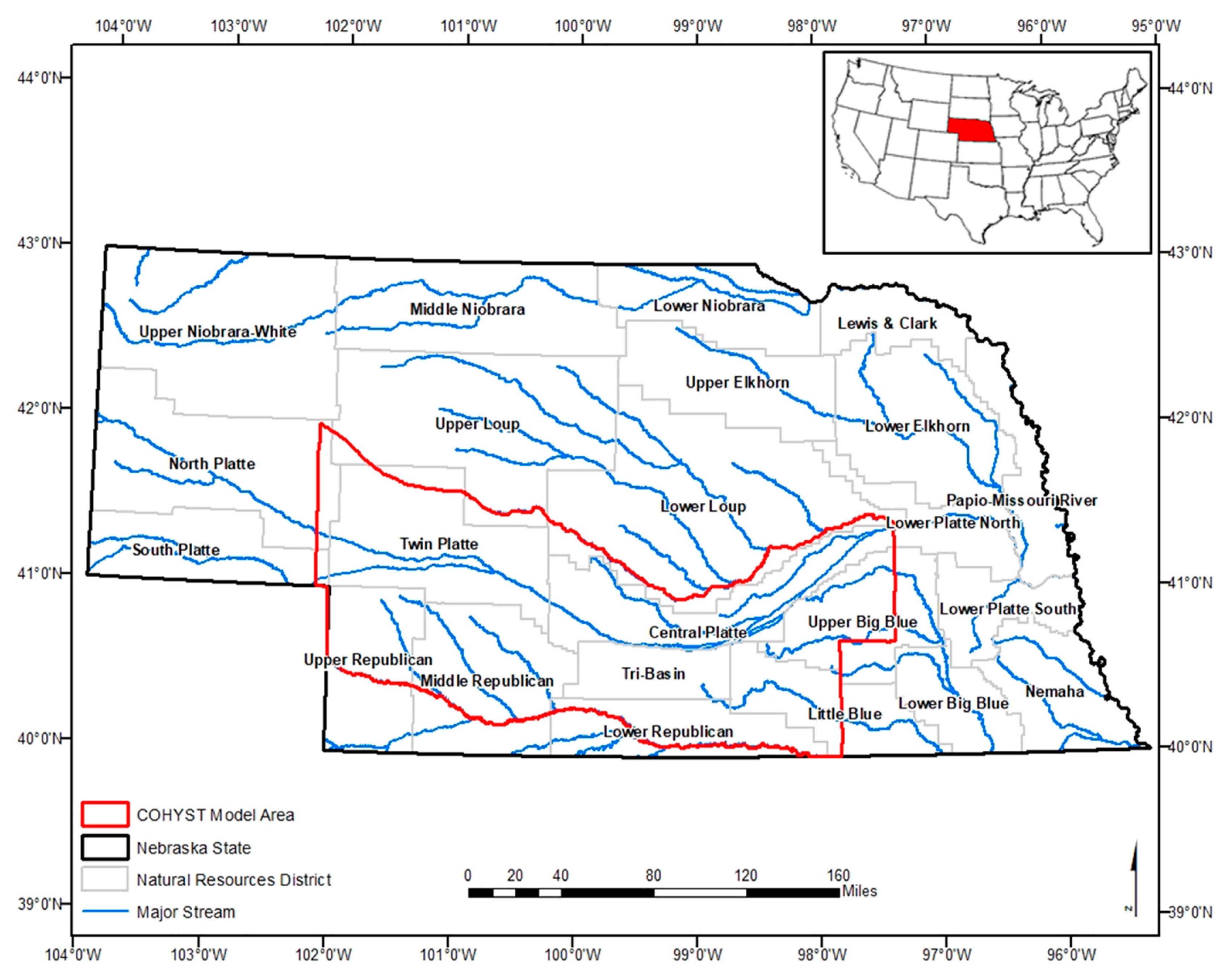
Figure 2.
Sampled irrigated (355) and non-irrigated (464) groundtruth fields across the COHYST region during the 2014 growing season.
Figure 2.
Sampled irrigated (355) and non-irrigated (464) groundtruth fields across the COHYST region during the 2014 growing season.
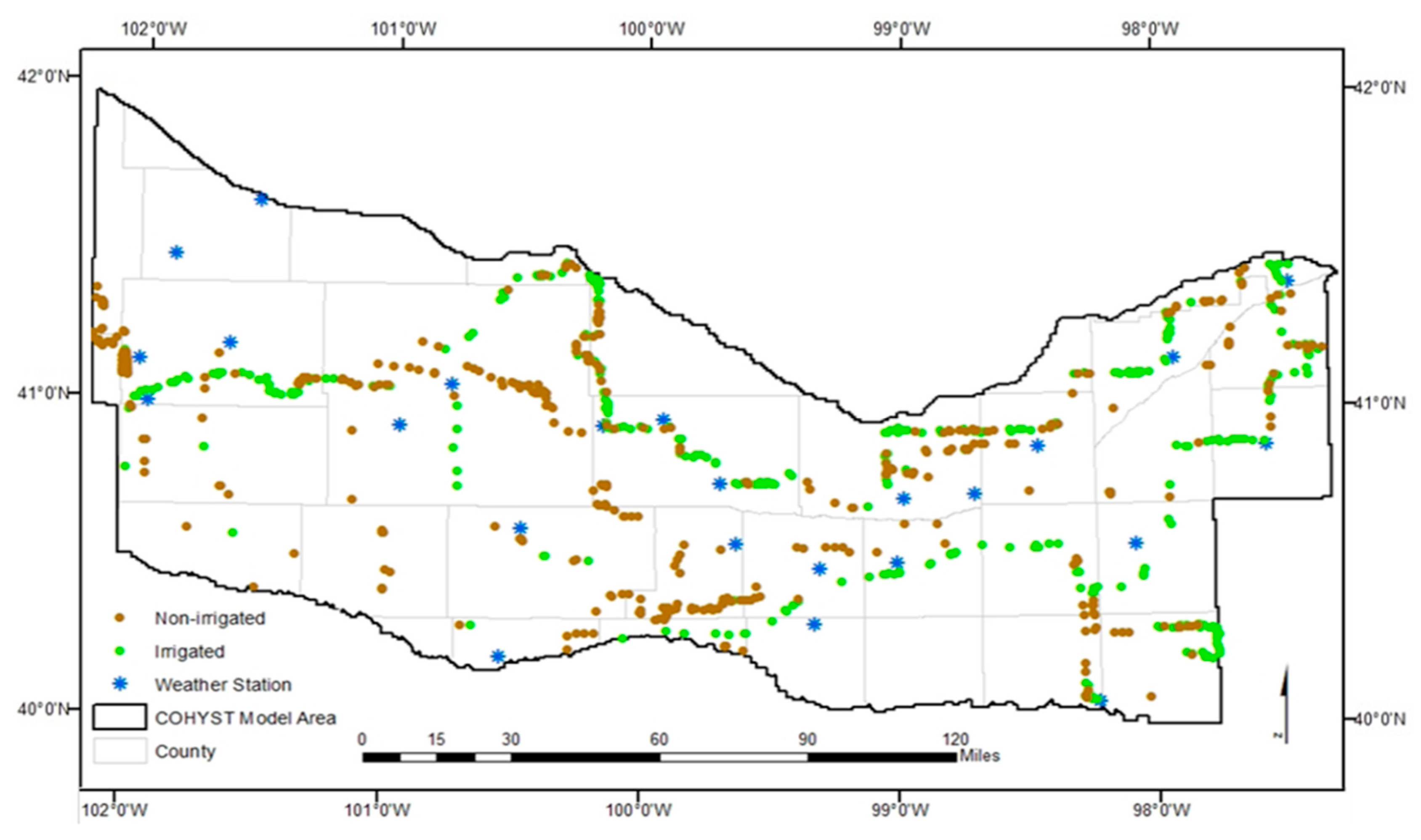
Figure 3.
Nebraska precipitation average for the months of June, July, and August from 1980 to 2017; 1901–2000 mean precip (μ: 239.3 mm); and the standard deviations (σ: 2.11 mm) about the mean. Data source: http://www.ncdc.noaa.gov/cag/time-series/us.
Figure 3.
Nebraska precipitation average for the months of June, July, and August from 1980 to 2017; 1901–2000 mean precip (μ: 239.3 mm); and the standard deviations (σ: 2.11 mm) about the mean. Data source: http://www.ncdc.noaa.gov/cag/time-series/us.
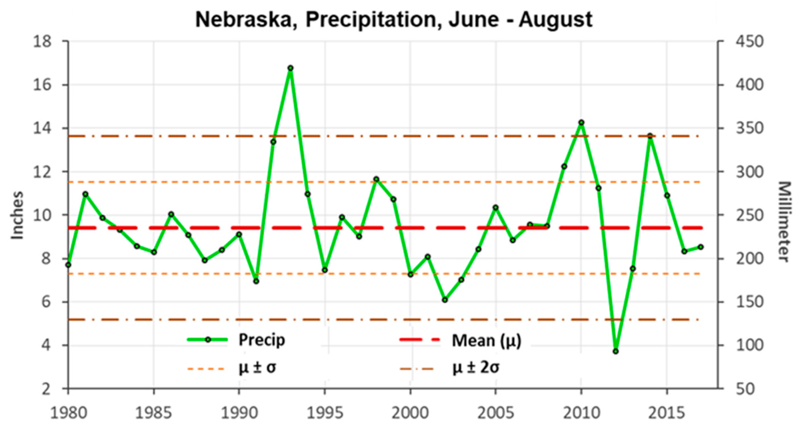
Figure 4.
Empirical distributions of NGI and EGI indices for all fields combined (Irrigated and non-irrigated areas), irrigated, and non-irrigated areas. Redlines indicate the threshold values of NGI and EGI.
Figure 4.
Empirical distributions of NGI and EGI indices for all fields combined (Irrigated and non-irrigated areas), irrigated, and non-irrigated areas. Redlines indicate the threshold values of NGI and EGI.

Figure 5.
Empirical distributions of NGI index for irrigated and non-irrigated areas after the classification scheme has been applied.
Figure 5.
Empirical distributions of NGI index for irrigated and non-irrigated areas after the classification scheme has been applied.
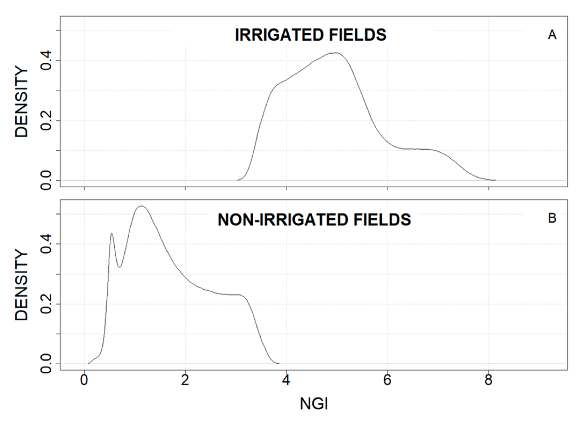
Figure 6.
NDVI-Evaporation Fraction-Green Index (NEG) Irrigation classification scheme flow diagram. Thd = Threshold.
Figure 6.
NDVI-Evaporation Fraction-Green Index (NEG) Irrigation classification scheme flow diagram. Thd = Threshold.

Figure 7.
Spatial distribution of NEG derived irrigated fields in the COHYST model region during the growing season of 2010 (A) and 2015 (B). Crop types derived from NASS CDL.
Figure 7.
Spatial distribution of NEG derived irrigated fields in the COHYST model region during the growing season of 2010 (A) and 2015 (B). Crop types derived from NASS CDL.
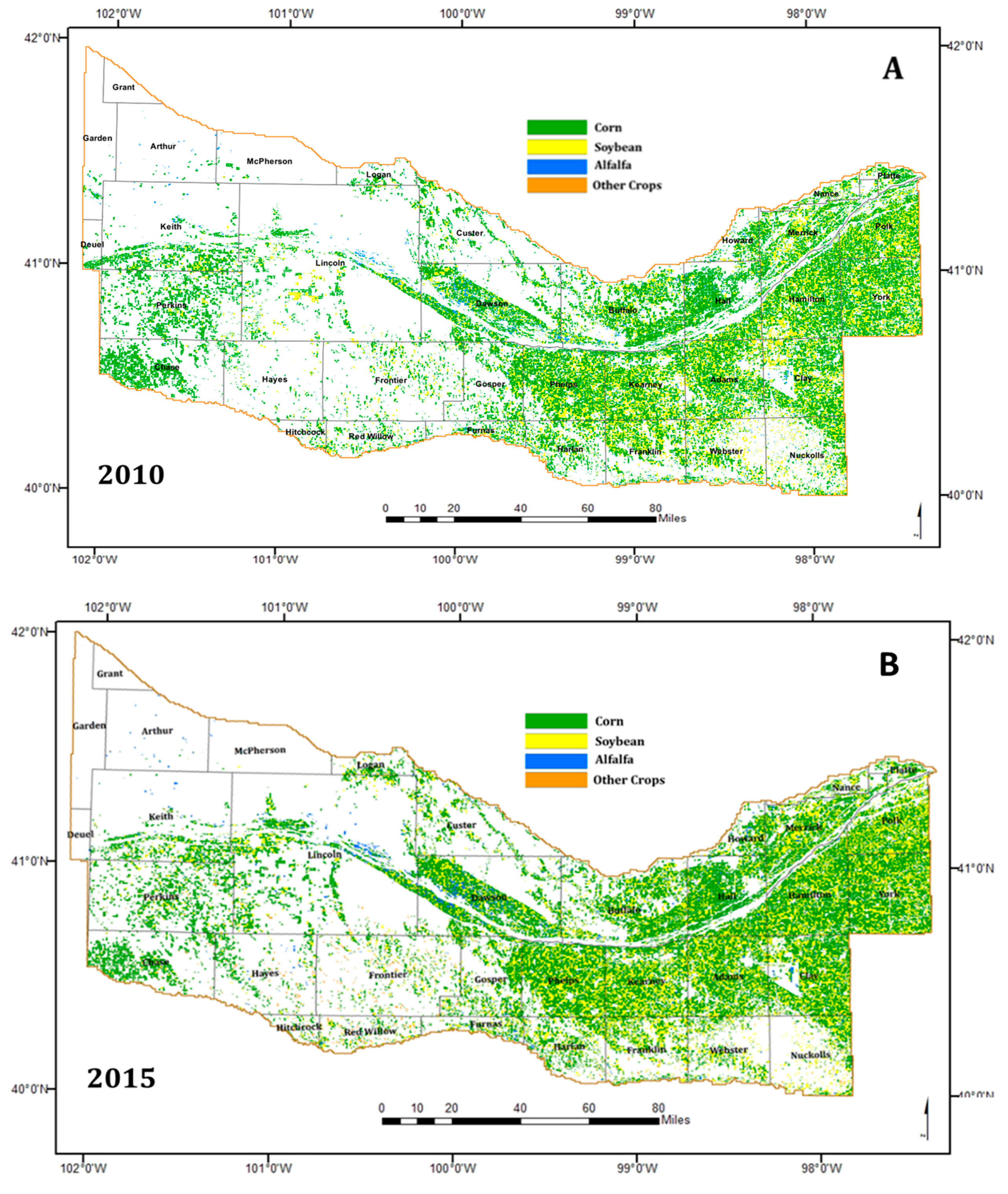
Figure 8.
Normal rainfall distribution across the COHYST region during the growing season (June, July and August). Base period: 1981–2010. Data source: Prism [40].
Figure 8.
Normal rainfall distribution across the COHYST region during the growing season (June, July and August). Base period: 1981–2010. Data source: Prism [40].
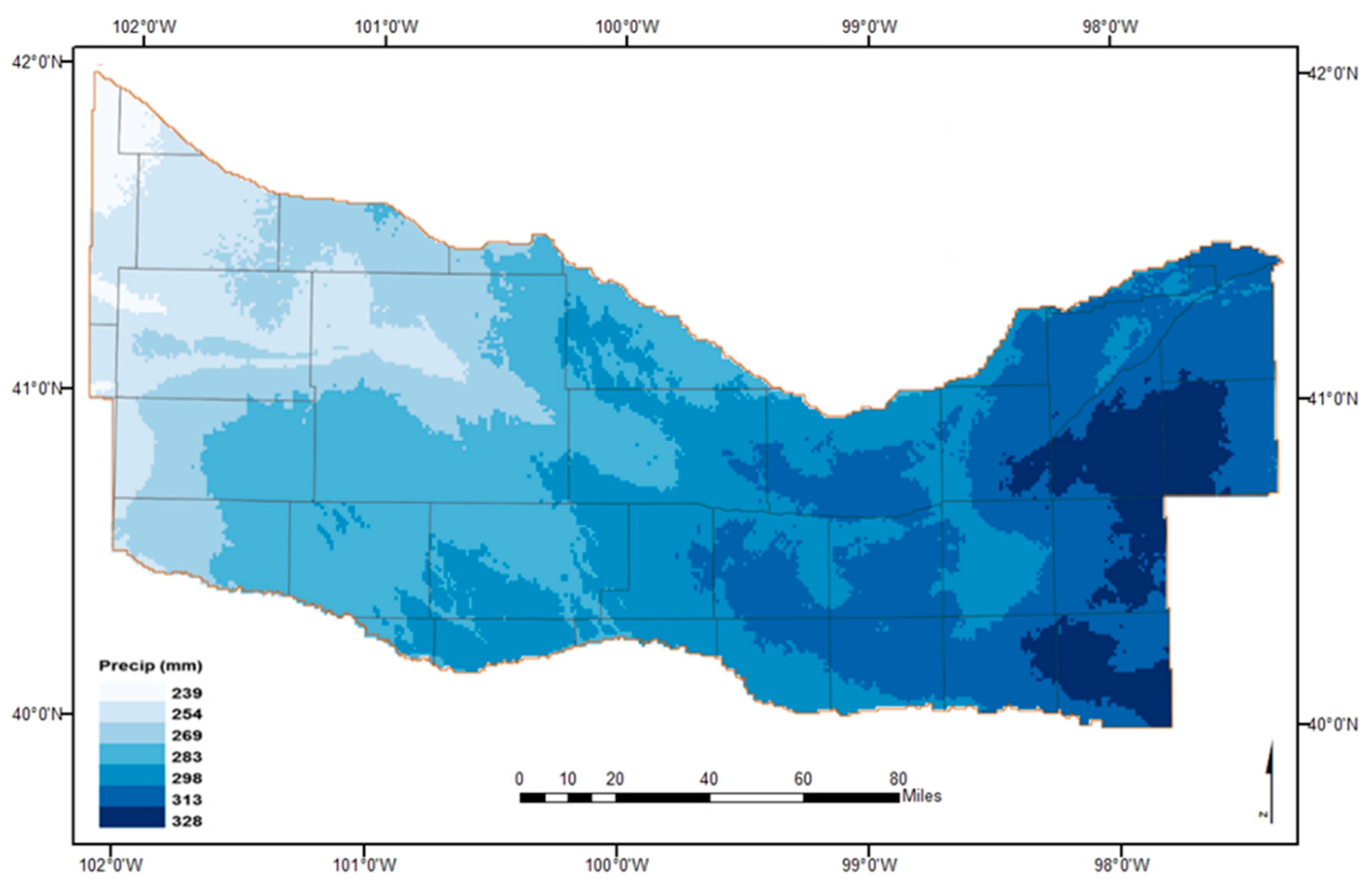
Figure 9.
Regression between NASS and NEG irrigated area by county for 2010 and 2015.

Figure 10.
Seasonal profile of NGI (A) and EGI (B) for irrigated and non-irrigated soybean and corn during the 2014 growing season. Each data point is an average of nine contiguous pixels of a square. DOY denotes Day of Year.
Figure 10.
Seasonal profile of NGI (A) and EGI (B) for irrigated and non-irrigated soybean and corn during the 2014 growing season. Each data point is an average of nine contiguous pixels of a square. DOY denotes Day of Year.

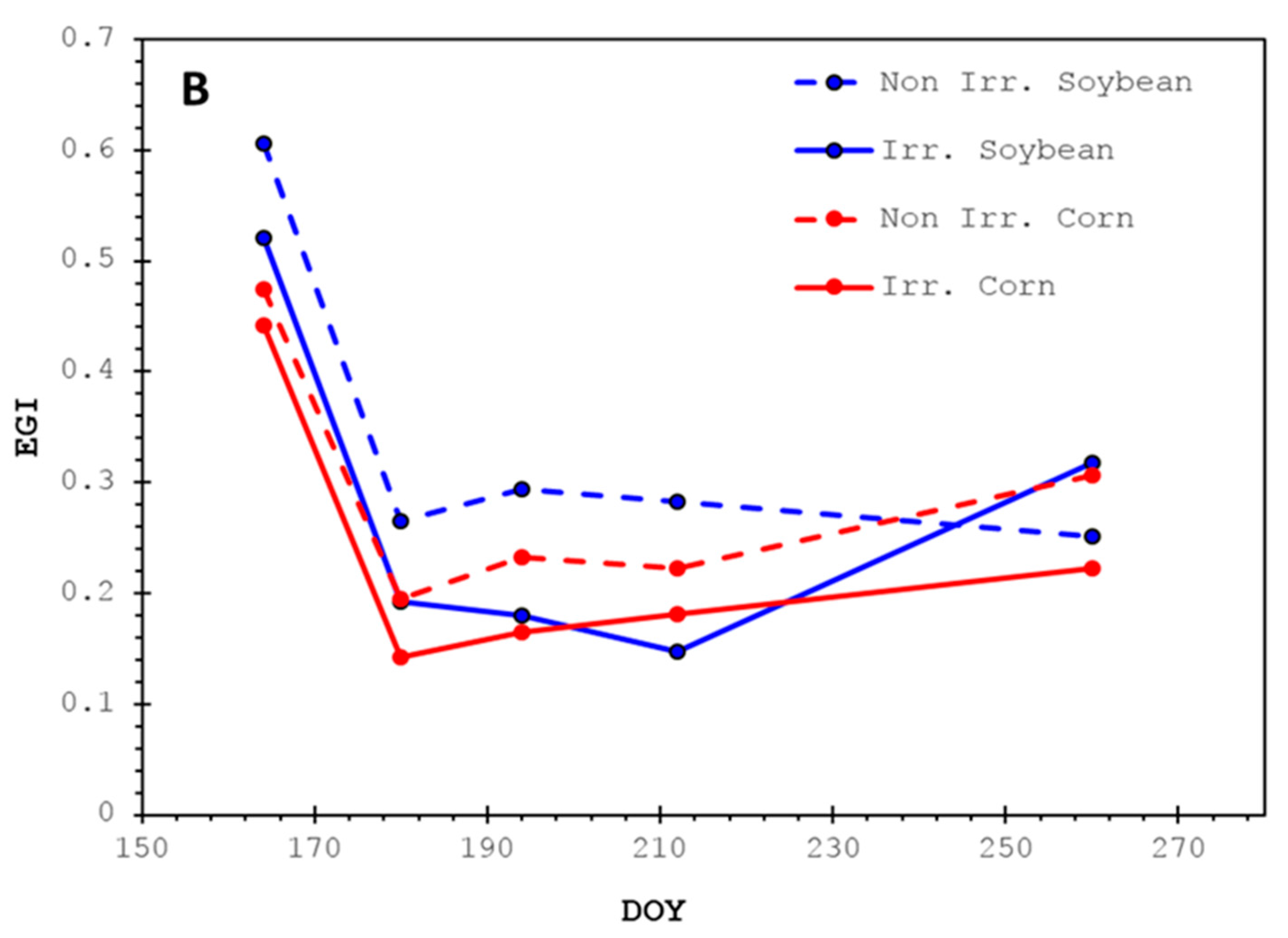
Table 1.
Results of error matrix and Kappa analysis between NEG scheme and groundtruth data from the 2010, 2014, and 2015 growing seasons.
Table 1.
Results of error matrix and Kappa analysis between NEG scheme and groundtruth data from the 2010, 2014, and 2015 growing seasons.
| Year | Irrigation Status | Producer’s Accuracy (%) | User’s Accuracy (%) | Overall Accuracy (%) | Kappa Value |
|---|---|---|---|---|---|
| 2010 | Irrigated | 90 | 92 | 87 | 0.70 |
| Non-irrigated | 81 | 77 | |||
| 2014 | Irrigated | 98 | 88 | 91 | 0.82 |
| Non-irrigated | 83 | 96 | |||
| 2015 | Irrigated | 93 | 71 | 88 | 0.72 |
| Non-irrigated | 86 | 97 |
Table 2.
NEG COHYST estimated irrigated acreages (ha) and percentage from total irrigated acreages for the main crops grown in COHYST model region in 2015 growing season.
Table 2.
NEG COHYST estimated irrigated acreages (ha) and percentage from total irrigated acreages for the main crops grown in COHYST model region in 2015 growing season.
| Crop | 2010 | 2015 | ||
|---|---|---|---|---|
| Area (ha) | % Area | Area (ha) | % Area | |
| Corn | 979,246 | 67.0 | 1,093,569 | 68.0 |
| Soybean | 446,856 | 30.6 | 456,255 | 28.0 |
| Alfalfa | 35,902 | 2.5 | 34,665 | 2.1 |
Table 3.
Coefficient of determination (R2), MAPE and RMSE between NASS and NEG estimated county irrigated area for 2015 and 2010.
Table 3.
Coefficient of determination (R2), MAPE and RMSE between NASS and NEG estimated county irrigated area for 2015 and 2010.
| STATS | 2015 | 2010 |
|---|---|---|
| R2 | 0.99 | 0.98 |
| MAPE (%) | 7.48 | 6.30 |
| RMSE (ha) | 6829.40 | 4625.00 |
© 2017 by the authors. Licensee MDPI, Basel, Switzerland. This article is an open access article distributed under the terms and conditions of the Creative Commons Attribution (CC BY) license (http://creativecommons.org/licenses/by/4.0/).
Share and Cite
MDPI and ACS Style
Pun, M.; Mutiibwa, D.; Li, R. Land Use Classification: A Surface Energy Balance and Vegetation Index Application to Map and Monitor Irrigated Lands. Remote Sens. 2017, 9, 1256. https://doi.org/10.3390/rs9121256
AMA Style
Pun M, Mutiibwa D, Li R. Land Use Classification: A Surface Energy Balance and Vegetation Index Application to Map and Monitor Irrigated Lands. Remote Sensing. 2017; 9(12):1256. https://doi.org/10.3390/rs9121256
Chicago/Turabian StylePun, Mahesh, Denis Mutiibwa, and Ruopu Li. 2017. "Land Use Classification: A Surface Energy Balance and Vegetation Index Application to Map and Monitor Irrigated Lands" Remote Sensing 9, no. 12: 1256. https://doi.org/10.3390/rs9121256
Note that from the first issue of 2016, this journal uses article numbers instead of page numbers. See further details here.