Co-Orbital Sentinel 1 and 2 for LULC Mapping with Emphasis on Wetlands in a Mediterranean Setting Based on Machine Learning

Abstract

This study aimed at evaluating the synergistic use of Sentinel-1 and Sentinel-2 data combined with the Support Vector Machines (SVMs) machine learning classifier for mapping land use and land cover (LULC) with emphasis on wetlands. In this context, the added value of spectral information derived from the Principal Component Analysis (PCA), Minimum Noise Fraction (MNF) and Grey Level Co-occurrence Matrix (GLCM) to the classification accuracy was also evaluated. As a case study, the National Park of Koronia and Volvi Lakes (NPKV) located in Greece was selected. LULC accuracy assessment was based on the computation of the classification error statistics and kappa coefficient. Findings of our study exemplified the appropriateness of the spatial and spectral resolution of Sentinel data in obtaining a rapid and cost-effective LULC cartography, and for wetlands in particular. The most accurate classification results were obtained when the additional spectral information was included to assist the classification implementation, increasing overall accuracy from 90.83% to 93.85% and kappa from 0.894 to 0.928. A post-classification correction (PCC) using knowledge-based logic rules further improved the overall accuracy to 94.82% and kappa to 0.936. This study provides further supporting evidence on the suitability of the Sentinels 1 and 2 data for improving our ability to map a complex area containing wetland and non-wetland LULC classes.

1. Introduction

Land use and land cover (LULC) consists of fundamental characteristics of the Earth’s system intimately connected with many human activities and the physical environment [1]. Information on LULC is of key importance in environmentally or ecologically protected ecosystems or native habitat mapping and restoration (Council Directive, 92/43/EEC, 1992). Wetlands in particular represent one of the world’s most important and productive ecosystems, having a critical role in climate change, biodiversity, hydrology, and human health [2,3]. Wetlands include permanent water bodies, lands that remain completely dry over several months, and areas where water is below a dense vegetation cover, such as peat bogs or mangroves [4]. Those also include important natural complex habitat types such as fresh water marsh and riverine forests, scrublands, as well as agricultural landscapes [5]. Although freshwater wetlands cover only 1% of the Earth’s surface, these areas provide shelter to over 40% of the world’s flora and fauna species [6]. As such, wetlands are internationally recognized as an indispensable resource for humans [2] providing a wide range of services that are dependent on water, such as freshwater, agricultural production, fisheries and tourism [7].

Despite their importance, wetlands are one of the most threatened ecosystems due to anthropogenic factors such as intensive agricultural production, irrigation, water extraction for domestic and industrial use, urbanization, infrastructure, industrial development and pollution [7,8,9]. Many wetlands are under pressure due to the natural and anthropogenic climate change (namely, changes in rainfall patterns and temperature and extreme events [9], as well as changes in land use brought by increasing populations and urban expansion). Environmental concerns on the degradation of wetlands came to the fore during the Ramsar Convention [8]. Over the last century, it is estimated that 50% of the world wetlands have disappeared, with an increased rate of 3.7 times that during the 20th and 21st centuries [10]. Thus, mapping and monitoring their dynamics over time is of crucial importance, as well as in the broader context of quantifying the temporal and spatial patterns of land use/land cover (LULC) and of its changes [11].

Earth Observation (EO) offers a repeated and frequent coverage of the Earth’s surface over long time periods, which is ideal for monitoring wetlands [8]. This has resulted in EO becoming the preferred method for natural resource managers and researchers [12]. Identification and characterization of key resource attributes allows resource managers to monitor landscape dynamics over large areas, including those where access is difficult or hazardous, and also facilitates extrapolation of expensive ground measurements for monitoring and management [13]. LULC mapping using satellite or airborne images allows for short- or long-term change detection and monitoring in such vulnerable habits [14,15,16].

Use of Synthetic Aperture Radar (SAR) imagery has been highly effective in wetland mapping and, although they are less frequently used in land-cover classification studies than optical data, they can be an important alternative or complementary data source [17]. Synergistic use of optical data with SAR imagery may enhance the wetland-related information. This is because SAR provides data associated with the inundation level, biomass, and soil moisture, complimentary to optical sensors’ information [18]. In this context, Sentinel-1 offers dual-polarimetric C-band data and Sentinel-2 offers a wide range of high resolution spectral bands, thus testing their synergistic capability is of crucial importance.

Many studies have focused on mapping wetlands utilizing different band manipulation methods (e.g., Tasseled Cap (TC), Normalized Difference Water Index (NDWI), and Normalized Difference Vegetation Index (NDVI)) and image analysis techniques (e.g., Principal Component Analysis (PCA) and Minimum Noise Fraction (MNF)) for assisting image classification [19,20,21,22]. Thus far, most studies have been based on a single-date image, neglecting the seasonal phenology that a lake can have [8]. Recent studies published have explored the use of advanced machine learning classification algorithms, such as Support Vector Machines (SVMs), random forests (RFs), decision trees (DTs) and artificial neural networks (ANNs) for LULC mapping [15,16,17,23,24,25,26,27,28,29,30].

Although spectral information about ground objects is important in information extraction from remote sensing data, previous studies have indicated that texture features are also important for differentiating wetland classes [15,16,31,32,33,34,35]. Spectral features describe the tonal variations in different bands, whereas texture features describe the spatial distribution [36]. The most commonly used texture features are first order measurements (minimum, maximum, mean, range, standard deviation, skewness, and kurtosis) and second order measurements (mean, angular second moment, contrast, correlation, homogeneity, dissimilarity, variance, and entropy). First order statistics are used to quantify the distribution properties of the images’ spectral tone for a given neighborhood, while second-order statistics contain the frequency of co-occurring gray scale values and are calculated from the gray-level co-occurrence matrix (GLCM) [15].

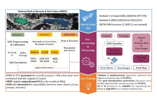
The recent growth of EO technology has resulted to the launch of sophisticated instruments such as that of the Sentinels series from the European Space Agency (ESA). This has opened up opportunities for new techniques development which aim at improving our ability to map wetland ecosystems. The Sentinel Mission is part of Copernicus Programme for monitoring climate change, natural resources management, civil protection and disaster management. Copernicus open data are available at Copernicus Open Access Hub (https://scihub.copernicus.eu/). Sentinel-1 (S1) is a Synthetic Aperture Radar (SAR) mission, providing data regardless of weather conditions and cloud coverage. Sentinel-2 (S2) is a land monitoring mission part of the Copernicus Program that provides high-resolution optical imagery to perform terrestrial observations in support of land services. The mission provides a global coverage of the Earth’s land surface every five days and at a spatial resolution of 10, 20 and 60 m, making the data of great use in studies related to land use/cover mapping and quantification of its changes. The Sentinel satellites can play a vital role in future land surface monitoring programs. Thus, exploring and evaluating the use of Sentinel data for wetland mapping is a thematic area of key interest and priority to develop. The improved discrimination capabilities offered by S1 and S2 and their effectiveness for wetland mapping combined with contemporary classification algorithms (e.g., Support Vector Machines (SVMs)) would therefore be important to be investigated.

This study aims at exploring the synergistic use between a range of spectral information products derived from Sentinel 1 and 2 and the SVMs classifier in evaluating their ability to map a complex area containing wetland and non-wetland LULC classes. In particular, the study objectives are: (1) to analyze a number of secondary derivatives produced from S2 data with the SVMs to evaluate their added value in mapping LULC and specifically wetlands; and (2) to investigate the suitability of S2 data and their synergistic use with S1 data with contemporary LULC mapping techniques (SVMs and knowledge rules) for LULC mapping with emphasis on mapping wetlands.

2. Materials and Methods

2.1. Study Site

The National Park of Koronia and Volvi Lakes (NPKV) lies in the Mygdonia basin, a semi-urban area located in a tectonic depression in northern Greece (Figure 1). The basin includes a large lowland area around the lakes that offers abundant soil for cultivation, as well as some mountain ranges at its borders. The rugged terrain creates a dense hydrographic network that ends up in the lakes. Climate is typical Mediterranean and annual rainfall ranges from 400 to 450 mm, distributed almost entirely during the winter season [37]. The wide rainfall range causes floods during the winter and serious droughts during the summer. The area is characterized by relatively low temperature during winter, ranging between −10 °C and 17 °C, whereas summer is warm with temperature ranging between 12 °C and 42 °C. NPKV is one of the most important Ramsar wetlands of Greece [38]. According to the Greek Biotope/Wetland Centre (http://www.ekby.gr/ekby/en/), many flora and fauna reproduce, nest, feed and rest in the wetland habitat. Two perennial plane trees between the lakes are characterized as “Monument of Nature” and provide shelter to numerous bird species. It is a significant habitat of structural and species diversity, also providing an important nesting and roosting site for many endangered bird species (e.g., Milvus migrans, Haliaeetus albicilla and Hieraaetus pennatus) [5]. In addition, 19 amphibian and reptile species, 34 species of mammals (some of them are under protection such as Myotis bechsteini, Myotis blyth, Lutra lutra, Canis aureus, Lutra lutra, Canis lupus and Capreolus capreolus) and 24 species of fish (among them, the rare “Aspius aspius”) live and reproduce within the area.

The wetland is protected by numerous national and international conventions due to its high environmental interest. It is also included in the European ecological network of protected sites “NATURA 2000”. Koronia Lake is a very important ecosystem of Greece which is almost vanishing because of non-sustainable water management practice in the region. It faces serious environmental issues, such as decreasing water levels, deterioration of water quality and water salinization [38]. The ongoing unsystematic economic growth of the area has resulted in water depletion and environmental degradation with serious social and economic impacts.

2.2. Datasets

Sentinel data were acquired from Copernicus Open Access Hub (https://scihub.copernicus.eu/). The selection was based on the following criteria: (1) low cloud coverage for Sentinel 2 images; (2) coincidence of at least one Sentinel 1 and Sentinel 2 image; and (3) seasonal coverage. According to these, the images selected were a Single Look Complex (SLC) Sentinel-1 (C-band) image captured on 2 August 2016 in Interferometric Wide Swath Mode (IW), a Sentinel 2 image also captured on 2 August 2016 and a Sentinel 2 image captured on 28 January 2016 (

Table 1. Summary of the characteristics of the remotely sensed datasets used in this study.

Sensor Name	Sensor Type	Acquisition Date	Band Information	Resolution (m)
Sentinel 1	C-band Radar	2 August 2016	VV + VH	5 × 20
Sentinel 2	Optical	2 August and 28 January 2016	490–2190 nm	10–20
SRTM	C/X-band Radar	2005	DEM	30

).

SLC product produces a 250 km swath at approximately 5 × 20 m resolution. The acquired imagery was obtained in dual-polarization mode at VV + VH. Sentinel 2 imagery was acquired in processing Level-1C which includes radiometric and geometric corrections, ortho-rectification and spatial registration on a global reference system with sub-pixel accuracy.

Additionally, a digital elevation model (DEM) of the area was obtained from the Shuttle Radar Topography Mission (SRTM) [39] and auto-downloaded from the Sentinel Application Platform (SNAP, v5.0) (Table 1). The DEM version 2 (released on 2005) (https://www2.jpl.nasa.gov/srtm/ (accessed on 24 June 2016)) was used with a spatial resolution of 30 m (1 arc-second) (vertical and vertical accuracy at 16 m and 20 m respectively) [40].

3. EO Data Processing

3.1. Pre-Processing

The acquired S1 and S2 data were pre-processed using the SNAP open source software and georeferenced in the WGS84 coordinate system and UTM projection, zone 34.

S1 data first had to split to the study site extend, de-burst the sub-swaths and apply the precise orbit file to offer the highest geometric precision. A Refined Lee 7 × 7 speckle filter was applied after suggestions [35] and the σ⁰ outputs were terrain corrected using SNAP’s “Range Doppler Terrain Correction” algorithm with the SRTM 1 arc-sec DEM. H-Alpha (H-a) decomposition [41] was included, allowing for entropy and alpha derivatives to be extracted from the data. Finally, all data were resampled at 10 m using a bilinear method.

S2 data pre-processing included atmospheric correction to convert the Top-of-Atmosphere reflectance values (TOA) to corrected Bottom-of-Atmosphere reflectance values (BOA). For the atmospheric correction, ESA’s Sen2Cor plug-in was used. Sen2Cor is a processor for Sentinel-2 Level 2A product generation and formatting; it performs the atmospheric, terrain and cirrus correction of Top-Of-Atmosphere Level 1C input data. Sen2Cor creates Bottom-Of-Atmosphere, optionally terrain and cirrus corrected reflectance images, as well as Aerosol Optical Thickness, Water Vapor, snf Scene Classification Maps, and Quality Indicators for cloud and snow probabilities. Its output product format is equivalent to the Level 1C User Product. Subsequently, bands 1, 9 and 10 were removed from the dataset. Then, the image was resampled at 10 m using a bilinear method and was also subset to the study site extent.

The SRTM DEM (30 m) was processed using ArcGIS software. Topographic information, namely slope, aspect and elevation, were derived and then resampled at 10 m utilizing the cubic convolution resampling method to match the Sentinel-2 spatial resolution. The accuracy of the derived DEM and the co-registration accuracy with the Sentinel images was assessed by comparing on a cell-by-cell basis with some same scale reference vector data of the area. A positional accuracy within the sensor pixel range (i.e., <10 m) was achieved which was considered satisfactory.

3.2. Analysis of Spectral Features

Spectral bands of S2 from 2 to 8A, 11 and 12 were used for this study (Figure 2). The Principal Component Analysis (PCA) and Minimum Noise Fraction (MNF) transformation methods were implemented to decrease the high correlation between the spectral bands providing independent information. PCA is a classical statistical method for transforming attributes of a dataset into a new set of uncorrelated attributes called principal components (PCs) and it is used to reduce the dimensionality of a dataset, while still retaining as much of the variability of the dataset as possible [42]. The MNF is used to determine the inherent dimensionality of image data, to segregate noise in the data and to reduce the computational requirements for subsequent processing [43]. PCA components 1 to 3 and MNF components 1 to 5 were used in this study to compose the new image for classification (Figure 3). The used components contained over 98% of the original information.

In addition, the commonly used Normalized Difference Vegetation Index (NDVI) (Equation (1)) and the Normalized Difference Water Index (NDWI) (Equation (2)) were used in this study to help discriminate vegetation types and water surfaces (Figure 2). Bands 8 (NIR) and 4 (Red) were used to calculate NDVI according to the following equation:

$$\mathrm{NDVI}=\frac{{\mathrm{NIR}}_{B8}-R_{B4}}{{\mathrm{NIR}}_{B8}+R_{B4}}$$

(1)

Likewise, bands 8 (NIR) and 3 (Green) were used to calculate NDWI according to the following equation:

$$\mathrm{NDWI}=\frac{G_{B3}-{\mathrm{NIR}}_{B8}}{G_{B3}+{\mathrm{NIR}}_{B8}}$$

(2)

3.3. Analysis of Texture Features

Apart from the tone (spectral variation), satellite images also consist of texture (spatial variation) [36]. While spectral information is relatively easy to quantify, texture is more difficult as it involves measurements of variation in pattern, shape and size [44]. Texture is described mainly by histograms, the gray-level co-occurrence matrix (GLCM), local statistics, etc., with GLCM being the most often used [32]. In this study, four statistical indicators of texture information, namely homogeneity (HOM), dissimilarity (DIS), entropy (ENT) and angular second moment (ASM), were implemented (Figure 4). These indicators were selected as effective indicators for the texture description of different land cover types [35]. Texture measures are influenced by window size since the scale of the spatial patterns measured, is dependent on window size [45]. After several window size implementations, it was found that a window size of 7 × 7 pixels is suitable for the particular study site. The texture measures were applied on the NDVI index, PC3 and MNF—C5.

3.4. Analysis of Shape Features

Shape is one of the most useful features in a satellite image and is an important aid for the extraction of information about ground objects [32]. The methods for discovering shape information about ground objects include perimeter, area and other shape measurements [46]. From the visual interpretation of the images, it was found that the shapes of the crops were relatively small and rectangular, while the shape of natural vegetation had more irregular patterns. Therefore, crops can be discriminated from natural vegetation, besides their spectral differentiation, based additionally on the area and the near-rectangle shape. Thus, two shape indicators were used, namely rectangle fit and compactness. An image segmentation was preceded using the “edge method” with scale factor 40% and merge factor 80% to ensure that the segments would be right-side to avoid the confusion in the separation of land cover types, as well as the limitation the shape attributes of the features [47,48]. The segmentation was applied to red (R), green (G), blue (B), near-infrared (NIR) and NDVI bands to both summer and winter images to identify seasonal changes in crops (Figure 5).

3.5. Crop Features Extraction

To extract the crop features a combination of the previously mentioned methods was adopted. The segmented image (Figure 5) was used and a range of permitted values for both spectral and shape features was defined (

Table 2. Value range used for crop extraction.

	Attribute	Minimum	Maximum
Spectral mean	NDVI	0.3	0.9
	Slope	1.5	5.0
Shape indicator	Rectangle Fit	0.45	1.00
	Area	8000	800,000
	Compactness	0.005	0.035

). The values used for the extraction are shown in Table 2.

4. Wetlands Mapping from Sentinel

4.1. LULC Classes

The classification scheme used in this study was developed in two stages. In the first stage, land use land cover (LULC) classes were defined which were representative of the scene’s attributes for a particular image acquisition date (2 August 2016) (

Table 3. Implemented land use/land cover (LULC) classes (first stage).

LULC Classes	Class Description
Crops	Non-wetland class, healthy and high yield arable farming land
Water	Wetland class, exposed surface water
Artificial Surfaces	Non-wetland class, impervious surfaces, urban fabric, roads, industrial facilities
Forest	Non-wetland class, mixed forest with trees from medium to large size
Shrub	Non-wetland class, long or short grass species, sparse trees and bushes
Sand	Non-wetland class, exposed lake, river or estuarine bed, coarse sand
Soil	Non-wetland class, bare land, very low or no vegetation
Marshes	Wetland class, aquatic plants that are either emerge, submerge or floating in water
Swamps	Wetland class, aquatic forest or shrubs

).

In the second stage, a multi-seasonal approach was attempted to classify all important area’s attributes, thus both summer and winter multi-spectral images were used. LULC classes were selected based on knowledge about the specific area. For this purpose, “Crops” were divided into “Summer Crops”, “Winter Crops” and “Permanent Crops”, and a new class named “Grassland” was implemented. A set of training points were selected representative of each class.

4.2. Support Vector Machines

Support Vector Machines (SVMs) is a nonlinear and non-parametric large margin supervised machine learning classifier implementing Vapnik’s structural risk minimization principle [49]. SVMs have several advantages in comparison to other hard classification approaches (for an overview of SVMs uses, see [50]). SVMs separate the samples of different classes by finding the separating hyperplane related to maximal margin minimizing the hinge loss function. Such solution guarantees a minimal generalization error. Essentially, the hyperplane is the decision surface on which the optimal class separation takes place. Intuitively, a good separation is achieved by the hyperplane that has the largest distance to the neighboring data points of both classes. Each training example is represented by a feature vector. To avoid computational overload, this is not done by evaluating all training points, but only a subset, called the “support vectors” of the algorithm.

By using nonlinear kernel functions (e.g., Gaussian RBF and polynomial), the SVMs implicitly work linearly in a higher dimensional space, corresponding to a nonlinear solution in the input space, where the data naturally exist. Such mapping into the higher dimensional kernel space is implicitly performed by applying a kernel function k(·,·), evaluating the dot product between samples mapped in some higher dimensional space as φ(x_i)′φ(x_j), where ′ denotes vector transpose. For the standard binary SVMs formulation implemented in this paper, the hyperplane f(x) = w′x + b optimally separating the two classes is found by minimizing:

$$\begin{array}{c}mi{n}_{w,b,\xi }\frac{1}{2}||w||+C{\displaystyle \sum }_{i=1}^N{\xi }_i\\ \\ s.t.w^{\prime }x+b⩾1-{\xi }_i\\ \\ {\xi }_i⩾0,i=1,\dots ,N\end{array}$$

(3)

The slack variables ξ allow some training errors, guaranteeing robustness to noise and outliers. C corresponds to a user selected parameter to control the complexity of the model, acting as a trade-off parameter between nonlinearity and number of training errors. This quadratic optimization is solved by introducing Lagrange multipliers α to obtain the following dual form:

$$\begin{array}{c}ma{x}_{\alpha }{\displaystyle \sum }_{i=1}^N{\alpha }_i-\frac{1}{2}{\displaystyle \sum }_{i=1}^N{\alpha }_i{\alpha }_j{y}_i{y}_{j}k\left(x_i,x_j\right)\\ s.t. 0⩽{\alpha }_i⩽C,{\displaystyle \sum }_{i=1}^N{\alpha }_i{y}_i=0\end{array}$$

(4)

When the optimal solution of the latter optimization is found, i.e., the α, labels of unknown samples x^t are predicted by the side of the margin in which they lie, i.e., by the following expression:

$$\widehat{y}=sign\left(f\left(x^t\right)\right)=sign\left({\displaystyle \sum }_{i=1}^N{\alpha }_{i}k\left(x_i,x^t\right)\right)$$

(5)

Note that standard SVMs are sparse in the α coefficients, so the final solution may be equivalently expressed only by the samples having a non-zero α. These samples are the ones lying on the separating margins f(x) = 1 and f(x) = −1.

To represent more complex hyperplane shapes than the linear methods, the techniques can be extended by using kernel functions. In this case, the problem transforms into an equivalent linear hyperplane problem of higher dimensionality. The use of the kernel function essentially allows the data points to be classified to spread in a way that allows the fitting of a linear hyperplane. Commonly used SVMs kernels include polynomial and radial basis function (RBF), and sigmoid kernels. In addition, SVMs also introduces a cost parameter C to quantify the penalty of misclassification errors in order to handle non-separable classification problems. In this study, RBF kernel was used for performing the pair-wise SVMs classification due to its promising capabilities compared to linear and polynomial [23]. RBF kernel is defined from the following equation:

Radial Basis Function:

$$K(x_i,x_j)=\exp (-\gamma {\Vert (x_i,x_j)\Vert }^2),\gamma >0$$

(6)

This kernel requires the definition of only a small number of input parameters (i.e., the C and γ parameters) and has also already been shown to produce generally good results in a range of classification studies (e.g., [29,30,51]). SVM optimum parameters of the classification implementation were established. The γ value was kept as suggested, 1/number of features. After several tests, the optimum C value was found at 2000 (Figure 6). From a C value of 1, overall accuracy rapidly rose up to 500 before beginning to plateau at 2000.

After parameter selection, the entire scene was classified with the entire dataset tested. For the classification, different scenarios were implemented aiming at assessing the added value of the different derivatives generated in the previous processing steps. All scenarios included NDVI, NDWI and elevation, as their contribution is considered to be effective in recent studies [52,53,54]. Initially (SB), only the original S2 channels were used. The first scenario (T) examined the performance of the transformed images without the original channels. In the second scenario (T + SB), the contribution of the transformed channels to the overall classification accuracy was examined using them along with the initials. The third scenario (SAR) examined the contribution of the S1 data derivatives. The fourth scenario (GLCM) examined the contribution of the texture characteristics resulting from the GLCM. Finally, in the fifth scenario (MS), a seasonal approach was examined, using features from both the summer and the winter images. The process was repeated until all components were examined and in each case, the channels that appeared to contribute to the increase in accuracy were also used in the following scenarios.

4.3. Post-Classification Corrections

Although LULC maps reached high accuracies, each scenario was found promising for different purposes. For example, the multi-seasonal approach (MS) contributed in the improvement of the classification accuracy in vegetation classes more, while sand/soil and impervious surfaces were better differentiated when the texture features were used (GLCM) (

Table 4. The different scenarios tested were grouped in six main thematic categories.

	v2.0	v2.1	v2.2	v2.3	v2.4	v2.5
Spectral Bands (SB)	X		X	X	X	X
Transformations (T)		X	X	X	X	X
SAR				X	X	X
GLCM					X	X
Multi-seasonal (MS)						X

). A post-classification refinement was developed and applied using the LULC maps and ancillary information built in a hypothesis framework of Knowledge Engineer (ERDAS Imagine, 2016) to reduce classification errors. The process involves the definition of hypotheses and variables, as well as the implementation of true/false rules in a detailed decision tree (Figure 7). The variables in the decision tree classifier refer to a band of data, while the terminal hypotheses represent the final classes of interest. A decision tree is a type of multistage classifier that can be applied to a stack of images designed to implement decision rules. The tree is made up of a series of decisions that are used to determine the correct class for each pixel. The rules can be based on any available characteristic of the dataset. For example, additional elevation information was used in this study to assist the correct classification of vegetation types (i.e., forest–marshes). The classified images from previously implemented steps, along with the ancillary information (e.g., cloud mask, NDVI, NDWI, slope, elevation, and crop features), were used herein as variables.

4.4. Accuracy Assessment

Accuracy assessment was carried out by the overall accuracy (OA) (Equation (7)) and kappa (K) (Equation (8)) statistics. In addition, accuracy of each class was evaluated separately using User’s and Producer’s accuracy (UA and PA), to reveal if error was evenly distributed between classes or if some classes were classified more correctly or not. The detailed error matrix was also computed for each of the classification images, as it allowed evaluating the UA and PA accuracy for each of the information classes included in our classification scheme.

$$\mathrm{OA}={\sum }_{i=1}^k\frac{N_{ii}}{N}$$

(7)

$$\mathrm{Kappa}=\frac{n{{\displaystyle \sum }}_{i=1}^q{n}_{ii}-{{\displaystyle \sum }}_{i=1}^q{n}_{Ri}{n}_{Ci}}{n^2-{{\displaystyle \sum }}_{i=1}^q{n}_{Ri}{n}_{Ci}}\times 100$$

(8)

The selection of a sufficient number of training and validation samples, as well as their representativeness, is critical for proper classification [55]. Samples are typically collected from in-situ data, aerial photographs or very high resolution satellite images. In this study, Google Earth images (20 March 2017) were used for the validation along with field photographs. The samples were selected as groups of pixels (polygons and polylines) for each class. In total, 13,888 pixels (~0.2% of the total pixels) were selected for training samples and 20% of those (2777) for validation (

Table 5. Training and validation samples for each land use/land cover LULC class collected as group of pixels.

	Training	Validation
marshes	857	200
swamps	681	120
forest	2741	550
shrubs	853	170
crops	1457	300
sand	1188	200
soil	1493	300
urban	1862	370
water	2856	570

).

5. Results

5.1. Support Vector Machines

Regarding the overall classification accuracy, the curve ascended from 90.83% to 93.85% and kappa from 0.894 to 0.928, which indicates a strong agreement with reality (Figure 8). Some exceptions were observed when the initial S2 bands were removed. S2 bands seem to have the greatest contribution to the classification results. The most significant contribution to the accuracy of the classification appeared to be the texture features derived from the GLCM analysis and the seasonal approach for the vegetation classes. Overall, the highest accuracy (93.85%) was reached when the NDVI and MNF texture bands (entropy, homogeneity, dissimilarity, and angular second moment) were used. On the other hand, the lowest accuracies were observed when the PCA components were used alone (82.50%) and when the H-a dual decomposition derivatives were implemented (91.37%).

As mentioned above, each scenario’s results were promising for different LULC classes. Individual class accuracies in vegetation classes decreased (up to ~20%) when S2 red bands (B5, B6, B7, and B8A) were removed. S1 derivatives contributed mostly to distinguish bare ground and impervious surfaces. Texture derivatives increased class accuracies for both vegetation (2–5%) and bare ground classes (4–7%).

As shown in

Table 6. The User’s (UA) and Producer’s (PA) accuracies for all classes in the best scenario of each group. The six groups are: SB (Spectral Bands); T (Transformations); T + SB (Transformations + Spectral Bands); SAR (Synthetic Aperture Radar); GLCM (Texture features); and MS (Multi-seasonal).

		SB	T	T + SB	SAR	GLCM	MS
marshes	PA (%)	95.83	95.83	95.00	95.00	95.83	96.67
	UA (%)	61.17	56.65	62.64	62.98	66.86	68.24
swamps	PA (%)	78.00	70.50	78.50	78.50	83.50	82.50
	UA (%)	82.54	81.03	83.96	83.96	82.27	80.88
forest	PA (%)	99.64	99.64	99.64	99.64	99.64	98.73
	UA (%)	99.46	99.82	99.82	99.82	100.00	100.00
shrubs	PA (%)	97.65	99.41	98.82	98.82	98.82	98.24
	UA (%)	75.11	85.35	81.55	80.77	90.32	89.78
crops	PA (%)	69.67	70.00	72.00	72.33	74.33	73.67
	UA (%)	84.27	84.34	85.38	85.43	88.14	87.01
sand	PA (%)	100.00	94.50	100.00	100.00	100.00	100.00
	UA (%)	86.96	86.30	88.11	87.72	89.69	90.91
soil	PA (%)	93.33	91.00	92.67	92.33	96.33	96.33
	UA (%)	94.28	88.93	93.92	93.58	98.63	98.30
urban	PA (%)	77.30	77.57	81.62	80.81	91.62	93.51
	UA (%)	98.62	90.82	97.11	97.08	99.41	99.43
water	PA (%)	99.12	98.95	99.30	99.30	98.25	98.25
	UA (%)	99.82	99.82	99.47	99.47	99.82	99.82
Overall (%)		90.83	89.78	91.69	91.58	93.85	93.78
Kappa		0.89	0.88	0.90	0.90	0.93	0.93

, the main misclassified classes are “marshes” and “crops”, followed by “swamps” and “urban”. Producer’s and User’s accuracies (PA and UA) indicate that, while “swamps” ranged between ~70% and ~80% and “urban” between ~77% and ~93%, “crops” did not exceed 75% in any scenario tested. “Marshes” appears to be the most unreliable class, as many pixels misclassified as marshes (mainly crops). UA in “marshes” class was lower than 70% in all scenarios while PA was almost 95%. This means that, even though almost 95% of the reference marsh areas have been correctly identified as “marshes”, less than 65% of the areas identified as “marshes” in the classification were actually marshes. On the other hand, classes “water” and “forest” had the best results (>98.00%), as far as User’s and Producer’s accuracy (UA and PA) is concerned.

5.2. Post Classification

After the completion of the post-classification step, overall classification accuracy reached 94.82% and kappa coefficient 0.9362 (

Table 7. Overall accuracy (OA) and kappa coefficient after the post-classification and User’s and Producer’s accuracies (UA and PA) for all the classes.

OA (%)|Kappa		94.82%|0.9362
	water	marshes	swamps	forest	shrubs	grass
UA (%)	99.05%	94.37%	89.40%	79.32%	98.03%	96.47%
PA (%)	99.78%	85.59%	89.89%	97.06%	88.85%	95.85%
	crops s	crops w	crops p	urban	sand	soil
UA (%)	91.59%	97.25%	98.02%	95.59%	99.87%	88.53%
PA (%)	84.58%	96.50%	95.77%	80.90%	76.62%	99.38%

). All LULC classes were also classified with fairly high accuracy (for all classes, above 75%). For all vegetation classes, an accuracy above 80% was also reported (Table 7). The classes with the highest misclassification error are “urban”, “sand” and “soil”, while “forest” and “shrubs” appear to have some misclassification errors as well. Specifically, “shrubs”, “urban” and “sand” classes appear more unreliable, with relatively high commission error, which means a relatively low percentage of each class’s pixels actually represents the particular class on the ground. For “forest” and “soil”, higher omission error was reported, which indicates that a relatively low percentage of each class’s ground pixels also appears the same in the classified image.

6. Discussion

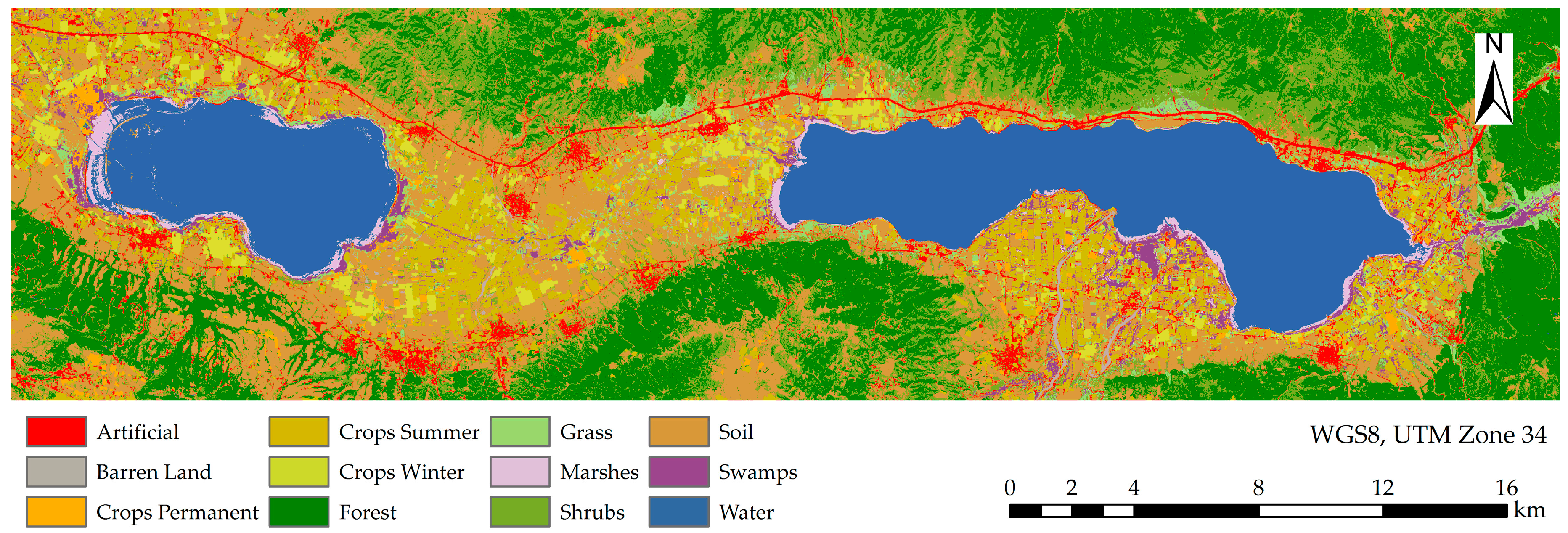
Accuracy assessment results suggest that the synergistic use of S1 and S2 data can achieve high classification accuracy, especially when combined with information on elevation, texture and shape. In a wetland area, the classes that prevail are water, aquatic vegetation and agriculture. In our case, water covers almost 15% of the area. The above, combined with the seasonality of both the lakes and the different types of vegetation, constitute a highly complex ecosystem in which the classification of LULC types may prove difficult. Moreover, weather conditions affect the quality of optical data (e.g., cloud cover) and the ground conditions (e.g., drought) affect the quality of SAR data, since it reduces the backscatter variations of the different classes due to their moisture difference. This is confirmed by both OA, UA and PA for specific classes. Wetland classes (especially marshes) were the most misclassified and the results were more accurate when texture and seasonality were considered.

Although vegetation classes have a similar spectral response, spectral signatures between some of the different LULC types can be distinguished in the red-edge area of the spectrum. That may explain the significant contribution of S2 red bands in the classification accuracy improvement. UA and PA for vegetation classes (marshes, swamps and crops) decreased significantly when S2 bands were removed (v2.1–T). Moreover, vegetation’s phenological cycle helped the separation of different types in the multi-seasonal approach. A difficulty in distinguishing the aquatic and the inland vegetation was also observed. Texture features helped in this respect, as indicated by several previous studies [35,56,57,58]. Crops were successfully separated from natural vegetation using shape features, which can be easily explained as the cultivated land has more regular patterns and shape than natural vegetation areas.

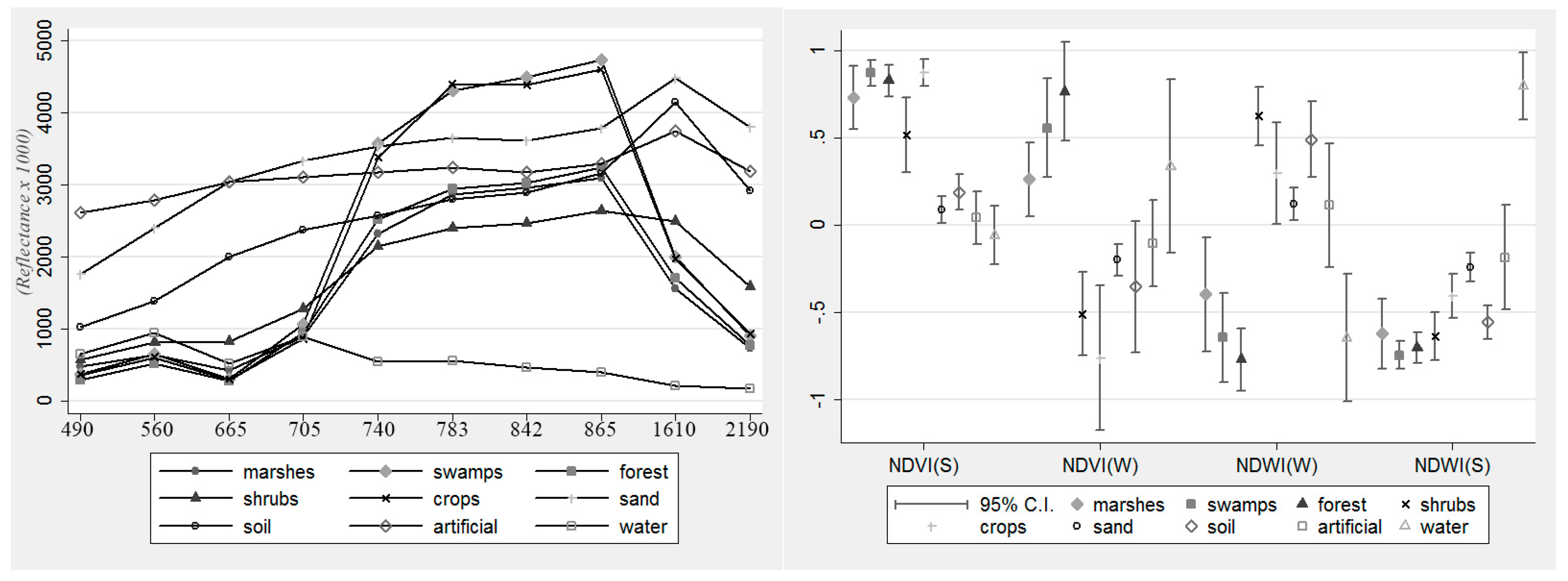
Spectral features showed to be less effective in the separation of artificial, soil and sand classes, which was possibly due to their low spectral separability (refer to Figure 2). While the first image was acquired in mid-summer, the presence of moisture is significantly low on the ground which can lead to high reflectance values and, thus, confusion between artificial surfaces and natural surfaces with no vegetation (soil, sand). Specifically, according to data collected from the Meteorological Station of Lagkadas (http://www.meteo.gr/meteoplus/index.cfm), the cumulative rainfall height for the previous month was only 6.0 mm, with temperature ranging between 14 °C (nighttime) and 38.8 °C (daytime). These weather conditions cause severe droughts to the area during the summer (see Section 2.1).

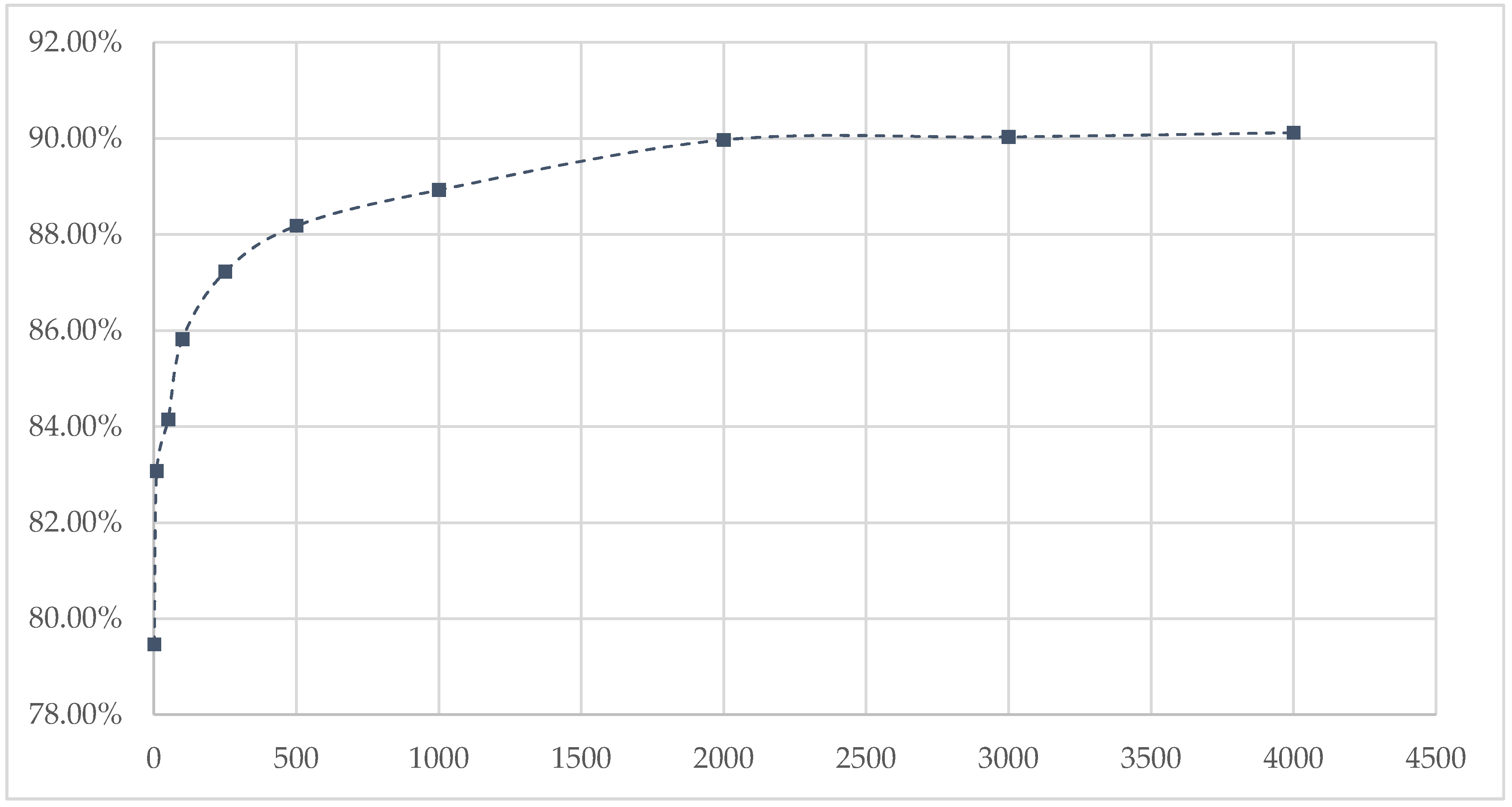
Findings reported herein also align with the other studies conducted independently using different multispectral satellite data underlining as well the promising capabilities of SVMs [23,24,59,60,61,62,63,64,65]. Evidently, a proper parameterisation can highly affect the SVMs performance [66,67]. The technique we chose to use in this study to parameterize the SVMs has been successfully implemented in other LULC investigations [27,68,69]. RBF kernel was used due to its promising capabilities as suggested by previous studies [23,50,68,70]. It is possible that another kernel function might have been more appropriate to the particular study site and data. SVMs algorithm achieved high classification accuracies, especially in wetland classes.

A number of studies have also indicated that SAR data may improve the classification accuracy, especially in extracting artificial classes (roads, buildings, etc.) [71,72] and change detection (wetland delineation, flood, etc.) [67,71,72,73]. However, in our study, S1 data slightly improved the classification accuracy, since the accurateness enhancement was about 1%. As mentioned above, weather conditions were not ideal at the specific time of the images acquisition, with high temperature and very low rainfall which had caused severe drought in the area. Although SAR data are only affected by wind speed, which in our case did not exceed 1.8 km/h (WSW direction), the severe drought conditions may have affected the data quality. Finally, the differences in the spatial resolution between the combined datasets and the image processing implemented to unify this spatial resolution could be another source of misclassifications reported herein.

Previous studies have indicated the improvement of accuracy in classifying land cover when knowledge rules are used [31,32,33]. In our study, post classification results achieved very high accuracy and indicated the efficiency of this method in producing a high-accuracy LULC map (Figure 9).

More broadly, the proposed methodology includes image analysis, extraction of key characteristics (e.g., texture) and usage of additional information (e.g., elevation) to compose a new dataset that will be used in the classification process. In this respect, findings of our study provide important assistance towards the development of relevant EO-based products not only in Greece (where the method was tested herein), but potentially also allowing a cost-effective and consistent long term monitoring of wetland/non-wetlands at different scales based on the latest EO sensing technology. With the provision of continuous, reliable spectral information from the ESA’s Sentinels 1 and 2 missions, the protraction of the proposed herein methodology has to some extend been assured. The proposed methodology may be easily transferred to be implemented at another location in terms of geographical scalability as well as in different wetland types (e.g., coastal wetlands, river estuaries, etc.). For this to be done successfully, the post-classification rules should be appropriately adapted when the method is implemented in different settings. The inclusion of this adjustment may both further improve the accuracy of the current technique and lead to a more detailed classification hierarchy. Finally, the present study also meliorates existing EU international figures, assisting efforts towards the development of operational products via the EU’s Copernicus service.

7. Conclusions

This study is, to our knowledge, among the first to investigate the combined use of Sentinel with advanced machine learning algorithms for LULC mapping with an emphasis on wetlands, particularly in a Mediterranean setting. Results showed that spatial, spectral and temporal resolutions of S2 data are suitable for classifying wetland areas. Overall accuracy using S2 bands alone reached 90.83% and kappa coefficient 0.894, which indicates a strong agreement with reality. The inclusion of S1 data did not significantly improve classification overall accuracy (<1%), at least this was the case in our study. However, the inclusion of additional spectral (NDVI, NDWI, PCA, and MNF), texture (GLCM) and shape indicators improved classification results, in some cases not significantly. Highest accuracies were achieved when the texture features (3%) where included, while the lowest when only selected transformed components were used (<0.5%). Cultivated land was successfully separated from natural using shape features. Finally, post classification techniques achieved very high overall accuracy (94.82%) with individual class accuracies more than 75% for all classes, thus providing an accurate map of the specific study site.

Wetlands are complex systems with a high presence of water and both natural and artificial surfaces. Thus, mapping wetlands and monitoring their changes over time is a challenging procedure, especially using multispectral imagery for this purpose. Sentinel missions can provide researchers and decision-makers invaluable data, with a satisfactory spatial and temporal resolution and, most importantly, free of charge. S2 proved to be appropriate for mapping such complex areas, thanks to the high spectral and spatial resolution of the data. Further work is required to verify the results obtained by testing the methods on other sites. The expansion of the techniques investigated herein using multi-seasonal as well as multi-annual datasets would also be another direction to be perhaps investigated next. Besides this, the use of other classifiers (e.g., random forests, artificial neural networks, etc.) would be an interesting avenue to be explored, as it may also provide information that can result in improving thematic information extraction accuracy from S1 and S2 satellites to map wetlands worldwide.

References

1. Aune-Lundberg, L.; Strand, G.-H. Comparison of variance estimation methods for use with two-dimensional systematic sampling of land use/land cover data. Environ. Model. Softw. 2014, 61, 87–97. [Google Scholar] [CrossRef]
2. Hu, S.; Niu, Z.; Chen, Y.; Li, L.; Zhang, H. Global wetlands: Potential distribution, wetland loss, and status. Sci. Total Environ. 2017, 586, 319–327. [Google Scholar] [CrossRef] [PubMed]
3. Ramsar Convention Secretariat. An Introduction to the Convention on Wetlands (Previously The Ramsar Convention Manual); Ramsar Convention Secretariat: Gland, Switzerland, 2016. [Google Scholar]
4. Tiner, R. Introduction to wetland mapping and its challenges. In Remote Sensing of Wetlands; Tiner, R.W., Lang, M.W., Klemas, V.V., Eds.; CRC Press: Boca Raton, FL, USA, 2015; pp. 43–66. [Google Scholar]
5. Kaiserli, A.; Voutsa, D.; Samara, C. Phosphorus fractionation in lake sediments—Lakes Volvi and Koronia, N. Greece. Chemosphere 2002, 46, 1147–1155. [Google Scholar] [CrossRef]
6. Mitra, S.; Wassmann, R.; Vlek, P.L.G. Global Inventory of Wetlands and Their Role in the Carbon Cycle; ZEF Discusson Papers on Development Policy; ZEF: Bonn, Germany, 2003; p. 57. [Google Scholar]
7. Russi, D.; Brink, P.; Farmer, A.; Badura, T.; Coates, D.; Förster, J.; Kumar, R.; Davidson, N. The Economics of Ecosystems and Biodiversity for Water and Wetlands; IEEP: London, UK, 2016. [Google Scholar]
8. Siachalou, S.; Doxani, G.; Tsakiri-strati, M. Time-series analysis of high temporal remote sensing data to model wetland dynamics: A hidden Markov Model approach. In Proceedings of the SENTINEL-2 for Science Workshop—ESA-ESRIN, Frascati, Italy, 20–22 May 2014. [Google Scholar]
9. Malak, D.A.; Hilarides, L. Guidelines for the Delimitation of Wetland Ecosystems; ETC-UMA: Málaga, Spain, 2016; pp. 1–23. [Google Scholar]
10. Davidson, N.C. How Much Wetland Has the World Lost? Long-Term and Recent Trends in Global Wetland Area. Mar. Freshw. Res. 2014, 65, 934–941. [Google Scholar]
11. Singh, S.K.; Srivastava, P.K.; Szabo, S.; Petropoulos, G.P.; Gupta, M.; Islam, T. Landscape transform and spatial metrics for mapping spatiotemporal land cover dynamics using Earth Observation data-sets. Geocarto Int. 2016, 1–15. [Google Scholar] [CrossRef]
12. Kennedy, R.E.; Townsend, P.A.; Gross, J.E.; Cohen, W.B.; Bolstad, P.; Wang, Y.Q.; Adams, P. Remote sensing change detection tools for natural resource managers: Understanding concepts and tradeoffs in the design of landscape monitoring projects. Remote Sens. Environ. 2009, 113, 1382–1396. [Google Scholar] [CrossRef]
13. Lamine, S.; Petropoulos, G.P.; Singh, S.K.; Szabó, S.; Bachari, N.E.I.; Srivastava, P.K.; Suman, S. Quantifying land use/land cover spatio-temporal landscape pattern dynamics from Hyperion using SVMs classifier and FRAGSTATS. Geocarto Int. 2017, 1–17. [Google Scholar] [CrossRef]
14. Bassa, Z.; Bob, U.; Szantoi, Z.; Ismail, R. Land cover and land use mapping of the iSimangaliso Wetland Park, South Africa: Comparison of oblique and orthogonal random forest algorithms. J. Appl. Remote Sens. 2016, 10, 15017. [Google Scholar] [CrossRef]
15. Szantoi, Z.; Escobedo, F.; Abd-Elrahman, A.; Smith, S.; Pearlstine, L. Analyzing fine-scale wetland composition using high resolution imagery and texture features. Int. J. Appl. Earth Obs. Geoinf. 2013, 23, 204–212. [Google Scholar] [CrossRef]
16. Szantoi, Z.; Escobedo, F.J.; Abd-Elrahman, A.; Pearlstine, L.; Dewitt, B.; Smith, S. Classifying spatially heterogeneous wetland communities using machine learning algorithms and spectral and textural features. Environ. Monit. Assess. 2015, 187, 262. [Google Scholar] [CrossRef] [PubMed]
17. Barrett, B.; Nitze, I.; Green, S.; Cawkwell, F. Assessment of multi-temporal, multi-sensor radar and ancillary spatial data for grasslands monitoring in Ireland using machine learning approaches. Remote Sens. Environ. 2014, 152, 109–124. [Google Scholar] [CrossRef]
18. Stratoulias, D.; Balzter, H.; Sykioti, O.; Zlinszky, A.; Tóth, V.R. Evaluating sentinel-2 for lakeshore habitat mapping based on airborne hyperspectral data. Sensors 2015, 15, 22956–22969. [Google Scholar] [CrossRef] [PubMed]
19. Baker, C.; Lawrence, R.L.; Montagne, C.; Patten, D. Change detection of wetland ecosystems using Landsat imagery and change vector analysis. Wetlands 2007, 27, 610–619. [Google Scholar] [CrossRef]
20. Wright, C.; Gallant, A. Improved wetland remote sensing in Yellowstone National Park using classification trees to combine TM imagery and ancillary environmental data. Remote Sens. Environ. 2007, 107, 582–605. [Google Scholar] [CrossRef]
21. Psomiadis, E.; Papazoglou, E.G.; Kafkala, I.; Antoniou, V. Sentinel-1 and -2 data for watershed and coastal area mapping: A case study from Central Greece. In Proceedings of the 2nd Conference on Geographic Information Systems and Spatial Analysis in Agriculture and the Environment, Athens, Greece, 25–26 May 2017. [Google Scholar]
22. Dong, Z.; Wang, Z.; Liu, D.; Song, K.; Li, L.; Jia, M.; Ding, Z. Mapping Wetland Areas Using Landsat-Derived NDVI and LSWI: A case study of West Songnen Plain, Northeast China. J. Indian Soc. Remote Sens. 2014, 42, 569–576. [Google Scholar] [CrossRef]
23. Kavzoglu, T.; Colkesen, I. A kernel functions analysis for Support Vector Machines for land cover classification. Int. J. Appl. Earth Obs. Geoinf. 2009, 11, 352–359. [Google Scholar] [CrossRef]
24. Otukei, J.R.; Blaschke, T. Land cover change assessment using decision trees, Support Vector Machines and maximum likelihood classification algorithms. Int. J. Appl. Earth Obs. Geoinf. 2010, 12 (Suppl. 1), 27–31. [Google Scholar] [CrossRef]
25. Szuster, B.W.; Chen, Q.; Borger, M. A comparison of classification techniques to support land cover and land use analysis in tropical coastal zones. Appl. Geogr. 2011, 31, 525–532. [Google Scholar] [CrossRef]
26. Petropoulos, G.P.; Knorr, W.; Scholze, M.; Boschetti, L.; Karantounias, G. Combining ASTER multispectral imagery analysis and Support Vector Machines for rapid and cost-effective post-fire assessment: A case study from the Greek wildland fires of 2007. Nat. Hazards Earth Syst. Sci. 2010, 10, 305–317. [Google Scholar] [CrossRef] [Green Version]
27. Zhang, C.; Xie, Z. Object-based vegetation mapping in the Kissimmee River Watershed using HyMap data and machine learning techniques. Wetlands 2013, 33, 233–244. [Google Scholar] [CrossRef]
28. Petropoulos, G.P.; Kalivas, D.P.; Griffiths, H.M.; Dimou, P.P. Remote sensing and GIS analysis for mapping spatio-temporal changes of erosion and deposition of two Mediterranean river deltas: The case of the Axios and Aliakmonas rivers, Greece. Int. J. Appl. Earth Obs. Geoinf. 2015, 35, 217–228. [Google Scholar] [CrossRef]
29. Petropoulos, G.P.; Kalivas, D.P.; Georgopoulou, I.A.; Srivastava, P.K. Urban vegetation cover extraction from hyperspectral imagery and geographic information system spatial analysis techniques: Case of Athens, Greece. J. Appl. Remote Sens. 2015, 9, 96088. [Google Scholar] [CrossRef]
30. Said, Y.A.; Petropoulos, G.P.; Srivastava, P.K. Assessing the influence of atmospheric and topographic correction and inclusion of SWIR bands in burned scars detection from high-resolution EO imagery: A case study using ASTER. Nat. Hazards 2015, 78, 1609–1628. [Google Scholar] [CrossRef]
31. Li, N.; Frei, M.; Altermann, W. Textural and knowledge-based lithological classification of remote sensing data in Southwestern Prieska sub-basin, Transvaal Supergroup, South Africa. J. Afr. Earth Sci. 2011, 60, 237–246. [Google Scholar] [CrossRef]
32. Zhang, R.; Zhu, D. Study of land cover classification based on knowledge rules using high-resolution remote sensing images. Expert Syst. Appl. 2011, 38, 3647–3652. [Google Scholar] [CrossRef]
33. Barkhordari, J.; Vardanian, T. Using post-classification enhancement in improving the classification of land use/cover of arid region (A case study in Pishkouh Watershed, Center of Iran). J. Rangel. Sci. 2012, 2, 521–534. [Google Scholar]
34. Visser, F.; Wallis, C.; Sinnott, A.M. Optical remote sensing of submerged aquatic vegetation: Opportunities for shallow clearwater streams. Limnologica 2013, 43, 388–398. [Google Scholar] [CrossRef]
35. Zhang, Y.; Zhang, H.; Lin, H. Improving the impervious surface estimation with combined use of optical and SAR remote sensing images. Remote Sens. Environ. 2014, 141, 155–167. [Google Scholar] [CrossRef]
36. Haralick, R.M. Statistical and structural approaches to texture. Proc. IEEE 1979, 67, 786–804. [Google Scholar] [CrossRef]
37. Alexandridis, T.K.; Zalidis, G.C.; Silleos, N.G. Mapping irrigated area in Mediterranean basins using low cost satellite Earth Observation. Comput. Electron. Agric. 2008, 64, 93–103. [Google Scholar] [CrossRef]
38. Perivolioti, T.; Mouratidis, A.; Doxani, G.; Bobori, D. Monitoring the Water Quality of Lake Koronia Using Long Time-Series of Multispectral Satellite Images; AUC Geographica: Praha, Czech Republic, 2016; Volume 54124, pp. 9–13. [Google Scholar]
39. Farr, T.G.; Rosen, P.A.; Caro, E.; Crippen, R.; Duren, R.; Hensley, S.; Kobrick, M.; Paller, M.; Rodriguez, E.; Roth, L.; et al. The Shuttle Radar Topography Mission. Rev. Geophys. 2007. [Google Scholar] [CrossRef]
40. Smith, B.; Sandwell, D. Accuracy and resolution of shuttle radar topography mission data. Res. Lett. 2003, 30. [Google Scholar] [CrossRef]
41. Cloude, S.R.; Pottier, E. An entropy based classification scheme for land applications of polarimetric SAR. IEEE Trans. Geosci. Remote Sens. 1997, 35, 68–78. [Google Scholar] [CrossRef]
42. Howley, T.; Madden, M.G.; O’Connell, M.L.; Ryder, A.G. The effect of principal component analysis on machine learning accuracy with high-dimensional spectral data. Knowl. Based Syst. 2006, 19, 363–370. [Google Scholar] [CrossRef]
43. Boardman, J.W.; Kruse, F.A. Automated spectral analysis: A geological example using AVIRIS data, north Grapevine Mountains, NevadaNo Title. In Proceedings of the ERIM Tenth Thematic Conference on Geologic Remote Sensing, San Antonio, TX, USA, 9–12 May 1994; pp. I-407–I-418. [Google Scholar]
44. Coburn, C.A.; Roberts, A.C.B. A multiscale texture analysis procedure for improved forest stand classification. Int. J. Remote Sens. 2004, 25, 4287–4308. [Google Scholar] [CrossRef]
45. Culbert, P.D.; Pidgeon, A.M.; St.-Louis, V.; Bash, D.; Radeloff, V.C. The impact of phenological variation on texture measures of remotely sensed imagery. IEEE J. Sel. Top. Appl. Earth Obs. Remote Sens. 2009, 2, 299–309. [Google Scholar] [CrossRef]
46. Shao, P.; Yang, G.; Niu, X.; Zhang, X.; Zhan, F.; Tang, T. Information extraction of high-resolution remotely sensed image based on multiresolution segmentation. Sustainability 2014, 6, 5300–5310. [Google Scholar] [CrossRef]
47. Liu, D.; Xia, F. Assessing object-based classification: Advantages and limitations. Remote Sens. Lett. 2010, 1, 187–194. [Google Scholar] [CrossRef]
48. Robson, B.A.; Nuth, C.; Dahl, S.O.; Hölbling, D.; Strozzi, T.; Nielsen, P.R. Automated classification of debris-covered glaciers combining optical, SAR and topographic data in an object-based environment. Remote Sens. Environ. 2015, 170, 372–387. [Google Scholar] [CrossRef]
49. Vapnik, V.N. The Nature of Statistical Learning Theory; Springer: New York, NY, USA, 1995. [Google Scholar]
50. Mountrakis, G.; Im, J.; Ogole, C. Support Vector Machines in remote sensing: A review. ISPRS J. Photogramm. Remote Sens. 2011, 66, 247–259. [Google Scholar] [CrossRef]
51. Petropoulos, G.P.; Kontoes, C.; Keramitsoglou, I. Burnt area delineation from a uni-temporal perspective based on Landsat TM imagery classification using Support Vector Machines. Int. J. Appl. Earth Obs. Geoinf. 2011, 13, 70–80. [Google Scholar] [CrossRef]
52. Chasmer, L.; Hopkinson, C.; Montgomery, J.; Petrone, R. A physically based terrain morphology and vegetation structural classification for wetlands of the Boreal Plains, Alberta, Canada. Can. J. Remote Sens. 2016, 42, 521–540. [Google Scholar] [CrossRef]
53. Maxwell, A.E.; Warner, T.A.; Strager, M.P. Predicting palustrine wetland probability using random forest machine learning and digital elevation data-derived terrain variables. Photogramm. Eng. Remote Sens. 2016, 82, 437–447. [Google Scholar] [CrossRef]
54. Serran, J.N.; Creed, I.F. New mapping techniques to estimate the preferential loss of small wetlands on prairie landscapes. Hydrol. Process. 2016, 30, 396–409. [Google Scholar] [CrossRef]
55. Lu, D.; Weng, Q. A survey of image classification methods and techniques for improving classification performance International Journal of Remote Sensing. Int. J. Remote Sens. 2007, 8, 823–870. [Google Scholar] [CrossRef]
56. Zhang, C.; Zang, S.; Liu, L.; Sun, Y.; Li, H. The application of support vector machine on Zhalong Wetland remote sensing classification research. In Proceedings of the 3rd International Conference on Computer Design and Applications (ICCDA 2011), Xi’an, China, 27–29 May 2011; Volume 2, pp. 255–260. [Google Scholar]
57. Hong, S.-H.; Kim, H.-O.; Wdowinski, S.; Feliciano, E. Evaluation of polarimetric SAR decomposition for classifying wetland vegetation types. Remote Sens. 2015, 7, 8563–8585. [Google Scholar] [CrossRef]
58. White, L.; Brisco, B.; Dabboor, M.; Schmitt, A.; Pratt, A. A collection of SAR methodologies for monitoring wetlands. Remote Sens. 2015, 7, 7615–7645. [Google Scholar] [CrossRef] [Green Version]
59. Elatawneh, A.; Kalaitzidis, C.; Petropoulos, G.P.; Schneider, T. Evaluation of diverse classification approaches for land use/cover mapping in a Mediterranean region utilizing Hyperion data. Int. J. Digit. Earth 2014, 7, 194–216. [Google Scholar] [CrossRef]
60. Volpi, M.; Petropoulos, G.P.; Kanevski, M. Flooding extent cartography with Landsat TM imagery and regularized kernel Fisher’s discriminant analysis. Comput. Geosci. 2013, 57, 24–31. [Google Scholar] [CrossRef]
61. Laurin, G.V.; Puletti, N.; Hawthorne, W.; Liesenberg, V.; Corona, P.; Papale, D.; Chen, Q.; Valentini, R. Discrimination of tropical forest types, dominant species, and mapping of functional guilds by hyperspectral and simulated multispectral Sentinel-2 data. Remote Sens. Environ. 2016, 176, 163–176. [Google Scholar] [CrossRef] [Green Version]
62. Petropoulos, G.P.; Partsinevelos, P.; Mitraka, Z. Change detection of surface mining activity and reclamation based on a machine learning approach of multi-temporal Landsat TM imagery. Geocarto Int. 2013, 28, 323–342. [Google Scholar] [CrossRef]
63. Petropoulos, G.P.; Arvanitis, K.; Sigrimis, N. Hyperion hyperspectral imagery analysis combined with machine learning classifiers for land use/cover mapping. Expert Syst. Appl. 2012, 39, 3800–3809. [Google Scholar] [CrossRef]
64. Gauci, A.; Abela, J.; Austad, M.; Cassar, L.F.; Zarb Adami, K. A Machine Learning approach for automatic land cover mapping from DSLR images over the Maltese Islands. Environ. Model. Softw. 2018, 99, 1–10. [Google Scholar] [CrossRef]
65. Fernández-Delgado, M.; Cernadas, E.; Barro, S.; Amorim, D.; Amorim Fernández-Delgado, D. Do we need hundreds of classifiers to solve real world classification problems? J. Mach. Learn. Res. 2014, 15, 3133–3181. [Google Scholar]
66. Gong, P.; Wang, J.; Yu, L.; Zhao, Y.; Zhao, Y.; Liang, L.; Niu, Z.; Huang, X.; Fu, H.; Liu, S.; et al. Finer resolution observation and monitoring of global land cover: first mapping results with Landsat TM and ETM+ data. Int. J. Remote Sens. 2013, 34, 2607–2654. [Google Scholar] [CrossRef]
67. Aslan, A.; Rahman, A.F.; Warren, M.W.; Robeson, S.M. Mapping spatial distribution and biomass of coastal wetland vegetation in Indonesian Papua by combining active and passive remotely sensed data. Remote Sens. Environ. 2016, 183, 65–81. [Google Scholar] [CrossRef]
68. Petropoulos, G.P.; Kalaitzidis, C.; Prasad Vadrevu, K. Support vector machines and object-based classification for obtaining land-use/cover cartography from Hyperion hyperspectral imagery. Comput. Geosci. 2012, 41, 99–107. [Google Scholar] [CrossRef]
69. Sonobe, R.; Tani, H.; Wang, X.; Kobayashi, N.; Shimamura, H. Parameter tuning in the support vector machine and random forest and their performances in cross- and same-year crop classification using TerraSAR-X. Int. J. Remote Sens. 2014, 35, 7898–7909. [Google Scholar] [CrossRef]
70. Erener, A. Classification method, spectral diversity, band combination and accuracy assessment evaluation for urban feature detection. Int. J. Appl. Earth Obs. Geoinf. 2012, 21, 397–408. [Google Scholar] [CrossRef]
71. Muro, J.; Canty, M.J.; Conradsen, K.; Hüttich, C.; Nielsen, A.A.; Skriver, H.; Remy, F.; Strauch, A.; Thonfeld, F.; Menz, G. Short-term change detection in wetlands using Sentinel-1 time series. Remote Sens. 2016, 8, 795. [Google Scholar] [CrossRef]
72. Qiu, L.; Du, Z.; Zhu, Q.; Fan, Y. An integrated flood management system based on linking environmental models and disaster-related data. Environ. Model. Softw. 2017, 91, 111–126. [Google Scholar] [CrossRef]
73. Schlaffer, S.; Matgen, P.; Hollaus, M.; Wagner, W. Flood detection from multi-temporal SAR data using harmonic analysis and change detection. Int. J. Appl. Earth Obs. Geoinf. 2015, 38, 15–24. [Google Scholar] [CrossRef]
Figure 1. The National Park of Koronia and Volvi Lakes (NPKV) lies in the Mygdonia basin, northern Greece. The detail shows the land uses according to Corine Land Cover (CLC) 2012.
Remotesensing 09 01259 g001
Figure 2. Spectral signatures of selected land use/land cover (LULC) classes (left). Vertical and horizontal axis represents the reflectance values (multiplied with scale factor of 10,000) of the Sentinel 2 summer image and the spectral bands used in this study in nanometers, respectively. Spectral mean values for Normalized Difference Vegetation Index (NDVI) and Normalized Difference Water Index (NDWI). Vertical axis represents the index values (right). The chart shows the values for the summer image (2 August 2016).
Remotesensing 09 01259 g002
Figure 3. Spectral mean values of: Principal Component Analysis (PCA) (left); and Minimum Noise Fraction (MNF) (right) components. Vertical axis represents the transformed values in both charts.
Remotesensing 09 01259 g003
Figure 4. Mean values of texture indicators. Vertical axis represents the texture values for Normalized Difference Vegetation Index (NDVI).
Remotesensing 09 01259 g004
Figure 5. A representative scene from the segmented image with both summer and winter crops using R, G, B, Near Infrared (NIR) and Normalized Difference Vegetation Index (NDVI) channels.
Remotesensing 09 01259 g005
Figure 6. C value selection graph for Support Vector Machines (SVM) plotted against the overall accuracy of the scene.
Remotesensing 09 01259 g006
Figure 7. The decision tree approach is based on series of decisions that are used to determine the correct class for each pixel. The chart shows the binary decisions implemented in this study.
Remotesensing 09 01259 g007
Figure 8. The figure above represents the overall accuracy. All Support Vector Machines (SVM)-based classifications were grouped into six groups according to the legend: SB, Spectral Bands; T, Transformations; MS, Multi Seasonal; GLCM, Texture Analysis and SAR, Synthetic Aperture Radar (as also shown in Table 4).
Remotesensing 09 01259 g008
Figure 9. The final classified image after the post-classification corrections (PCC).
Remotesensing 09 01259 g009