Ocean Wind and Wave Measurements Using X-Band Marine Radar: A Comprehensive Review


Department of Electrical and Computer Engineering, Memorial University of Newfoundland, St. John’s, NL A1B 3X5, Canada
*
Author to whom correspondence should be addressed.
Remote Sens. 2017, 9(12), 1261; https://doi.org/10.3390/rs9121261
Submission received: 13 November 2017
/
Revised: 1 December 2017
/
Accepted: 2 December 2017
/
Published: 5 December 2017
(This article belongs to the Section Ocean Remote Sensing)
Abstract
:Ocean wind and wave parameters can be measured by in-situ sensors such as anemometers and buoys. Since the 1980s, X-band marine radar has evolved as one of the remote sensing instruments for such purposes since its sea surface images contain considerable wind and wave information. The maturity and accuracy of X-band marine radar wind and wave measurements have already enabled relevant commercial products to be used in real-world applications. The goal of this paper is to provide a comprehensive review of the state of the art algorithms for ocean wind and wave information extraction from X-band marine radar data. Wind measurements are mainly based on the dependence of radar image intensities on wind direction and speed. Wave parameters can be obtained from radar-derived wave spectra or radar image textures for non-coherent radar and from surface radial velocity for coherent radar. In this review, the principles of the methodologies are described, the performances are compared, and the pros and cons are discussed. Specifically, recent developments for wind and wave measurements are highlighted. These include the mitigation of rain effects on wind measurements and wave height estimation without external calibrations. Finally, remaining challenges and future trends are discussed.
1. Introduction
Ocean wind and wave information is crucial for various on- and off-shore activities such as coastal construction, ship navigation, and marine resource development (e.g., mining and oil industries). Traditionally, wind and wave information has been obtained from anemometers and buoys, respectively. However, wind flow distortion due to the superstructure or the movement of the anemometer platform may affect wind measurements [1], and the employment of buoys may be limited by the surrounding environment [2]. Complementing the point measurements of such in-situ sensors, remote-sensing instruments such as synthetic aperture radar (SAR) [3,4,5], high frequency (HF) radar [6,7,8], and X-band marine radar [9,10,11,12] have been developed as alternative approaches over the last few decades. Particularly, X-band marine radar has been rapidly developed as an ocean remote sensor since it can image both the spatial and temporal variations of the sea surface with high resolutions. Furthermore, X-band marine radar is widely installed on ships for navigation purposes. If reliable wind and wave measurements can be obtained from such radars, the costs associated with traditional in-situ sensors such as anemometers and buoys can be significantly reduced. Thus, land-based or ship-borne X-band marine radar has garnered wide attention.
X-band marine radar generally operates at grazing incidence. Radar backscatter from the sea surface is primarily generated by Bragg resonance [9] interactions between the radar-transmitted electromagnetic microwaves and the high frequency gravity-capillary waves which are influenced by the effects of gravity and surface tension. For X-band radar operating with horizontal-transmit-horizontal-receive (HH) polarization, wedge scattering [13] and small-scale breaking waves [14] also play significant roles in radar backscattering.
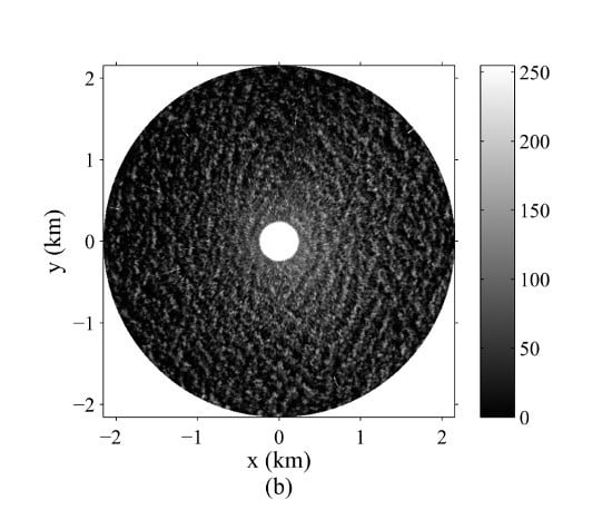
Since the sea surface roughness that causes the radar backscatter is induced by local winds, the dependence of the radar cross section (RCS) on wind speed [15] and the angle between radar look direction and wind direction [16] can be exploited to extract wind parameters from radar images [12]. On the other hand, long sea surface waves, including wind seas and swell, can be observed in radar images since they modulate radar backscatter signals. The modulations are mainly associated with hydrodynamic effects induced by interactions between capillary waves and long waves, tilt modulation due to the varying effective incidence angles of the radar signals along the slopes of long waves, and shadowing due to the obstruction of radar signals caused by higher waves [17]. The shadowing and tilt modulation are depicted in Figure 1a. Figure 1b is an example of radar image. Due to the modulations, wave parameters can be extracted from radar images [18,19,20].
Due to its high spatial and temporal resolutions, X-band marine radar has been used in many other oceanic applications, which involve target tracking [21], oil spill detection [22], internal wave analysis [23], wave group retrieval [24], surface current determination [25,26,27,28], upwelling observation [29], tide estimation [30], bathymetry mapping [31,32], surface elevation approximation [33,34] and prediction [35,36], coastal erosion [37], and detection of marine mammals [38]. In this paper, only the work related to sea surface wind and wave measurements is reviewed. The purpose of the review is to comprehensively compare the techniques developed for such measurements and to explore remaining challenges. Section 2 contains a review of the techniques for wind parameter extraction. The techniques for wave parameter extraction are reviewed in Section 3. Conclusions and an outlook for future trends appear in Section 4.
2. Wind Measurements
Due to the dependence of the radar cross section (RCS) on wind speed [15] and the angle between the radar look direction and the wind direction [16], X-band marine radar has been exploited to retrieve wind parameters [12]. Wind direction has generally been determined based on the fact that the backscatter of an HH-polarized X-band radar operating at grazing incidence presents only one peak in the upwind direction [39]. Wind speed has generally been determined by establishing a model relating wind speed to other parameters derived from radar images. The wind estimation methods can be classified as wind-streaks-based, image-intensity-variation-over-azimuth-based, and spectral-analysis-based.
2.1. Wind-Streaks-Based Techniques
Wind streaks are linear features first observed in SAR images for ocean surface wind direction estimation [40]. They are mainly caused by local turbulence, foam, and surfactants on the ocean surface. Such wind streaks are also visible in the temporally-integrated X-band marine radar images and aligned with the mean wind direction. Thus, they can also be used for wind measurements using X-band marine radar.
2.1.1. Local Gradients Method and Neural Network
The local gradients method (LGM) was originally proposed to extract wind-induced streaks from SAR images [41]. Dankert et al. [42,43,44] used LGM to determine wind direction as the orientation of wind-induced streaks from X-band marine radar images. Wind speed was estimated using a neural network (NN) that employed the mean normalized RCS (NRCS), radar-derived wind direction, and radar look direction as the input parameters, and wind speed as the output.
For wind direction estimation, the first step is to integrate a radar image sequence over time. Ocean surface wave signatures that show high variability in the time domain can then be removed. As a result, only static and quasi-static signatures of low frequencies, such as wind-induced streaks, remain visible in the integrated image. In the next step, the integrated image is subjected to repeated smoothing and sub-sampling, in which the image resolution is thrice decreased by a factor of 2, resulting in a so-called Gaussian image pyramid. Subsequently, local gradients are obtained from all the sub-sampled images with three different resolutions using the optimized Sobel operators [41], and the orientations of local wind streaks are determined to be those that are orthogonal to the local gradients. Then, wind direction is derived as the mean or the mode of all the determined local wind streak orientations. While a 180 ambiguity exists in the derived wind direction, it can be removed using the following techniques. The first technique is based on the cross-correlation function (CCF) of two temporally-integrated radar image sub-sequences. The moving distance and direction of image patterns can be indicated by the location of the CCF peak, thus removing the 180 ambiguity. The second technique is based on the cross-spectrum (CS) of the CCF. The movements of image harmonic features can be derived from the phases of the CS values for the corresponding wavenumbers of the harmonic components. Since the resulting motion directions of the image harmonic features are always within ±90 of the downwind direction, the 180 ambiguity can be removed. Another technique, based on the extraction of wind gusts visible in the image sequence [45], is discussed in Section 2.1.2. The scheme of the LGM for wind direction estimation is shown in Figure 2.
For wind speed determination, each temporally-integrated radar image over the range of 600 m or 900 m to 2100 m is divided into range-azimuth bins of 300 m in range and 5 in azimuth. The least inputs required for the NN involve the mean NRCS of the bins within ±15 in both cross-wind directions, the radar-retrieved wind direction and the radar look direction. The mean NRCS in the cross-wind directions is used for two reasons. Firstly, the NRCS is more sensitive to wind speeds in the cross-wind directions. Secondly, the NRCS in the upwind and downwind directions may be affected by blockage and wind shadowing due to neighbouring platforms, respectively. Improvements can be achieved if other parameters related to the sea state and atmospheric conditions are also included as the inputs of the NN. The sea state parameters include the signal-to-noise ratio (SNR), which is proportional to the square of significant wave height, and the peak wave phase speed, which can be calculated from peak wave frequency and peak wavenumber. The atmospheric conditions measured by external sensors include the air-sea temperature difference and the relative humidity.
In [42,43,44], two sets of data were used to test the techniques. The first dataset was collected from February to June 2001 on the platform Ekofisk 2/4 k located in the North Sea around 200 km off the west coast of Norway with wind speed up to 18 m/s. The second dataset was collected from August 2003 to November 2004, on the research platform FINO-I in the German Bight of the southern North Sea with wind speed up to 16 m/s. The comparison between in-situ and radar-derived wind directions showed a correlation coefficient of 0.99 and a standard deviation of 12.8∼14.2. For wind speed estimation, by including the atmospheric conditions (air-sea temperature difference and relative air humidity) as additional inputs, the standard deviation can be reduced by 0.12∼0.24 m/s. Good results for wind measurements have been obtained using this method. However, it may be difficult to apply the LGM to ship-borne radar data because ship motion may lead to less reliable estimation of the streak orientations from the temporally-integrated radar images. A preprocessing technique, such as georeferencing, may be required for its application to ship-borne radar data. For the NN technique, various input parameters are needed and a training process must be conducted.
2.1.2. Optical Flow-Based Motion Estimation
Dankert et al. [45] proposed an optical flow motion estimation-based technique (OFM) to retrieve wind fields from X-band marine radar images. This technique is based on the extraction of the movement of wind gusts that are visible in filtered and integrated images. Wind speed can be directly derived from the wind gusts without calibration.
Firstly, to filter out the ocean surface wave signatures, the linear dispersion relationship for surface gravity waves is applied to the 3D wavenumber-frequency spectrum of an image sequence. Next, a temporal moving average over 27 images is applied to a sequence of 32 images to remove high variability in the time domain, resulting in 5 averaged images , with and t being space and time coordinates, respectively. For each averaged image, the same smoothing and sub-sampling process as described in Section 2.1.1 is implemented to obtained the so-called Gaussian image pyramid. Then, wind gusts become visible in the resulting images. Based on a common assumption on optical flow, the intensity change in the averaged image is caused only by the motion of wind patterns. Thus, the total time derivative associated with equals zero, which results in [46]
where and are the spatial gradient and partial time derivative of the image intensity, respectively, T denotes the transpose of a matrix, and is the optical flow, with and being the components in the x and y directions, respectively. denotes the local wind velocity vector in this case. Under the assumption that the optical flow is constant within a local area and by using a local weighted least-squares technique [46], can be determined. In Equation (1), the first-order derivative of the image intensity with respect to space and time are calculated by optimized 3D Sobel operators [46]. Due to the application of 3D convolution (optimized 3D Sobel operators), the local wind velocity vector cannot be determined from the first and last images of the image sequence and the borders of images. Finally, all available estimated local wind velocity vectors are smoothed, and the mean wind velocity vector is determined as the mode of the smoothed local wind velocity vectors. A flowchart of the OFM is shown in Figure 3.
To test the technique, only 1332 data samples from the same dataset collected on the platform Ekofisk 2/4 k in the North Sea were used [45]. The correlation coefficient and standard deviation for wind direction measurements were 0.96 and 32.1, respectively, as compared to reference data from in-situ sensors. For wind speed measurements, the correlation coefficient and standard deviation were 0.64 and 2.68 m/s, respectively. It was observed that increasing the number of images involved in the moving average may improve the results. Although the technique does not require a calibration process, the accuracy of the results is relatively low compared to other methods. Also, as for the LGM, a preprocessing step, such as georeferencing, is required for ship-borne radar applications.
2.2. Intensity-Variation-Over-Azimuth-Based Techniques
As mentioned earlier, the variation of radar backscatter intensity over azimuth can also be exploited to retrieve wind direction. Other than the NN, wind speed can also be retrieved using an explicit model.
2.2.1. Curve Fitting (CF)-Based Methods
A. Single-CF
In [47], Lund et al. proposed a single-CF-based method for retrieving both wind direction and speed. Wind directions are extracted using a harmonic function that is least-squares fitted to the radar backscatter intensity as a function of azimuth. Wind speeds are determined from the average radar backscatter intensity using an empirical third-order polynomial obtained through training.
For HH-polarized X-band radar images collected at grazing incidence, only one backscatter intensity peak exists in the upwind direction [39]. This is the principle for wind direction estimation. First, radar backscatter intensities are averaged along each unobstructed azimuthal direction. Then, the average radar backscatter intensity as a function of the azimuthal direction is least-squares fitted by a cosine square function
where , , and are parameters determined through least-squares fitting. Wind direction is determined as the azimuthal direction corresponding to the peak of the fitted function. With least-squares fitting, wind directions can be retrieved even if the upwind direction appears in the obstructed portions of the image.
Wind speeds are retrieved by exploiting the dependence of radar backscatter intensity on wind speed. The overall average radar backscatter intensity of one radar image is calculated as the integration of the fitted function in Equation (2) over the full azimuth. This is expressed a
The fitted function in Equation (2) is used for calculating because it automatically fills the gaps in obstructed image portions. Then, a third-order polynomial relationship between and wind speed is assumed and trained using the wind speed data that are collected by external sensors such as anemometers. Based on the obtained third order polynomial, wind speed can be retrieved from for each individual radar image. The basic steps of the single-CF method for wind direction and speed retrieval are illustrated in Figure 4.
The datasets used to test the method were collected from R/V Roger Revelle travelling in the Philippine Sea near Taiwan island during two storms from 6 August to 9 August and from 12 September to 17 September 2010, respectively [47]. Test results show that the CF-based method works well for ship-borne X-band marine radar data, even if some portions of the radar image are obstructed by ship structures. Furthermore, only one parameter derived from radar data is needed to train the model function, significantly simplifying the wind speed estimation compared to the NN-based technique.
B. Dual-CF
Under low sea states, the overall image intensities are low, and this may lead to inaccurate wind estimation when using the CF-based method. Therefore, Liu et al. [48] modified the original CF-based method [47] with a dual-CF technique to improve wind direction and speed results under low sea state conditions.
In the dual-CF technique, an initial estimation of wind direction is first obtained by using the single-CF method. Then, to update the wind direction value, the radar data within ±60 of this estimated wind direction are employed for a second CF process. The range of ±60 is used because it is wide enough to include the actual wind direction and it is narrow enough to exclude low image intensities due to low sea states. For wind speed retrieval, negative values of the fitted function derived from the dual-CF technique are discarded from the integration in Equation (3) for the calculation of the average radar backscatter intensity .
To test the technique, two sets of data [48] were collected by two radars (Decca and Furuno) installed on the Canadian Navy research ship CFAV Quest during a sea trial in 2008 in the North Atlantic Ocean off the east coast of Canada while wind speed varied from 2 m/s to 16 m/s. Both the original CF-based method and the dual CF technique were applied to the two datasets. The dual-CF technique showed trivial improvements over the single-CF method with respect to the standard deviations of both wind direction and speed.
C. Two-Model-CF
In both the single-CF method and dual-CF technique, radar data collected in the presence of rain were excluded from wind estimation. This is because rain affects the radar backscatter and leads to less reliable wind estimation. Huang and Gill [11] proposed an algorithm to improve wind speed extraction from rain-contaminated radar images. Radar data contaminated by rain are first identified and extracted based on a parameter called zero-pixel percentage (ZPP). Then, the same third-order polynomial used for rain-free data in [47] are trained separately for the rain-contaminated data.
The algorithm was tested using the Decca radar data as mentioned in Section 2.2.1-B and [11]. The comparison between in-situ and radar-derived wind speeds using the two-model algorithm showed a standard deviation of 1.7 m/s, which is improved by 1.2 m/s compared to the results derived by using only one model for both rain-free and rain-contaminated radar data. However, in spite of the improvement of the wind speed estimation accuracy under rain conditions, the practicality of the algorithm is compromised by an additional procedure for distinguishing rain-free and rain-contaminated data and an extra training model.
2.2.2. Intensity Level Selection (ILS)-Based Methods
A. Original ILS
Vicen-Bueno et al. [49] proposed an ILS-based method for retrieving wind parameters from temporally-integrated and spatially-smoothed radar images. Wind direction is determined by searching for the maximum range for a selected intensity level along the azimuth, while wind speed is derived from the selected intensity level and its corresponding maximum range by training an empirical third-order polynomial geophysical model function.
In the first step, radar images are temporally integrated and spatially smoothed to remove high variabilities in the time and space domains, respectively. Then, a sequence of intensity levels is defined based on the image intensity range. For every azimuthal direction of each integrated and smoothed image, the maximum range with an intensity level equal to or greater than each defined intensity level is identified. Next, for each defined intensity level, the identified maximum ranges from all azimuthal directions are smoothed by a moving average over 5, and the lowest defined intensity level with all its associated smoothed maximum ranges being greater than an inner distance boundary is designated as the selected intensity level. Finally, the wind direction is determined as the azimuthal direction corresponding to the peak of the smoothed maximum ranges associated with the selected intensity level. After applying the above procedures to the first several integrated and smoothed images, rather than all the defined intensity levels, only the selected intensity level from the previous image and its upper and lower defined intensity levels are used for wind retrieval. This makes the algorithm more efficient.
Wind speed , which is estimated from the selected intensity level and the peak of smoothed maximum ranges associated with the selected intensity level, can be expressed as
with
where is the peak of smoothed maximum ranges associated with the selected intensity level , is the conversion rate between and , and , , , and are the parameters determined by least-squares fitting. For the training process, wind speed is measured by external sensors such as anemometers. After the training is completed, wind speed can be estimated from and for each individual integrated and smoothed radar image. Figure 5 depicts the basic steps of the method.
Datasets used to test this method were collected from the research platform FLIP at approximately 30 km northwest of Bodega Bay, California, USA, during four periods in June 2010 while wind speed varied from 4 m/s to 22 m/s [49]. As compared to reference values from anemometer data, the standard deviations of wind direction and speed results were 11 and 0.6 m/s, respectively, for the training data, and 14.3 and 0.8 m/s, respectively, for the test data.
B. Modified ILS
In the original ILS method, the obstruction of the radar field of view (FOV) and the appearance of islands may lead to less accurate results. Thus, Liu et al. [48] modified the original ILS method in [49] with blockage and island recognitions and an additional CF process, resulting in more robust wind direction and speed results when blockages or islands exist in the radar field of view.
First of all, blockages in the radar FOV due to obstruction by ship structures or other unknown factors are recognized. Blocked azimuthal directions are identified as those with ZPPs greater than 20%, and data in those directions are excluded from the ILS. Then, islands in the radar FOV are recognized as intensity bumps in the radar images. The intensity bump in each azimuthal direction is identified by applying the MATLAB built-in function, findpeaks. Data in the azimuthal directions in which islands are identified are also excluded from the ILS. Furthermore, an outer distance boundary is set for the ILS due to possible noise in the very far range. All smoothed maximum ranges associated with the selected intensity level should be smaller than the outer distance boundary. Finally, the harmonic function (2) is used to least-squares fit the smoothed maximum ranges to fill the gaps due to the exclusion of data. The azimuthal direction corresponding to the peak of the fitted function is determined as the wind direction and is further utilized for the wind speed determination which follows the original ILS procedure.
The same datasets as mentioned in Section 2.2.1-B were used to test the method [48]. After using the modified ILS method, the standard deviations of wind direction and speed were reduced by 4.9∼7 and 0.1∼0.3 m/s, respectively.
C. Texture-Analysis-Incorporated
Huang et al. [50] proposed a texture-analysis-incorporated (TAI) algorithm to extract wind parameters from rain-contaminated radar images. The TAI method first requires the identification of the rain-contaminated pixels in each azimuthal direction of radar images based on texture analysis. Then, only the data from the azimuthal directions in which the rain contamination is negligible are used to extract wind parameters by applying the modified ILS method.
The texture of a radar image is generated based on the calculation of intensity RMS difference. Next, the portion contaminated by rain is identified. If the number of pixels with intensities larger than a threshold (see [50]) is higher than or equal to 20 in one azimuthal direction in the texture image, that direction is considered as the one with negligible rain contamination and is retained. By this means, wave signatures can be retained in the image texture while rain clutter can be removed.
The Decca radar data as described in Section 2.2.1-B were also used for validating this method [50]. For rain-contaminated data, the standard deviations of wind direction and speed results are 19.9 and 2.0 m/s, respectively, by using the TAI method, and 34.4 and 3.3 m/s, respectively, without incorporating TAI.
2.2.3. Probability Distribution Function
Chen et al. [51] proposed a probability distribution function (PDF)-based method to retrieve nearshore sea surface wind vectors. With an adjustment for the influence of land, wind direction is also retrieved based on the azimuthal dependence of radar image intensity levels. Wind speed is determined from a model based on the PDF of radar image intensity levels and significant wave height, .
The method for wind direction retrieval is similar to single-CF. The first difference is that a sine function instead of (2) is used. In addition, the azimuthal direction corresponding to the peak of the fitted function, , is not regarded as wind direction directly but adjusted by an angle . This is because the appearance of two hills in the radar image, may not be the wind direction. An average is empirically obtained using the anemometer reference [51].
For wind speed retrieval, the expectation of the radar image intensity levels is calculated from the PDF of those levels. Then, a relationship between wind speed and as well as is sought through fitting
where , , and are parameters determined by the least-squares fitting process. In this model, the wind speed changes approximately linearly with under low sea state conditions, while the term mainly takes into account swell effects under high sea states. After the model is obtained, wind speed can be determined from and .
Datasets used to test the method were collected on Haitan Island, China, from October to December 2010 [51]. The data consisted of 535 radar image sequences and simultaneous anemometer and buoy measurements, and were divided into 10 groups based on corresponding wind speed values which ranged from 0 m/s to 20 m/s in increments of 2 m/s. One third of the data randomly selected from each interval were used for training the wind speed model, and the remainder were used for validating the model. An acceptable RMS difference of 26.2 for wind direction estimation was obtained while wind speeds ranged from 5 m/s to 20 m/s. For the data with wind speed varying from 0 m/s to 20 m/s, the RMS difference of wind speed retrieval results was 1.37 m/s. It was also found from the result that should be included in Equation (6) under moderate to high wind conditions.
2.3. Spectral-Analysis-Based Techniques
The methods described in Section 2.1 and Section 2.2 are based on the analysis of the spatial and temporal variations in the images. Another category of algorithms were designed mainly based on image spectral analysis.
2.3.1. Background Noise
Izquierdo and Soares [52] presented a method to retrieve wind speed from the background noise (BGN) of radar image sequences.
An image frequency-wavenumber spectrum is first obtained by applying the 3D discrete Fourier transform (DFT) to the radar image sequence. Then, spectral components corresponding to ocean waves and BGN are separated using the linear dispersion relationship for gravity waves. The total spectral energy of BGN, , is used to estimate wind speed based on the trained linear model [52].
Datasets used to test the method were collected close to the Port of Sines in Portugal, from September, 2000 to December, 2001 [52]. A radar image was divided into 36 directional sectors, each of which covers 10. The calibration was implemented for each directional sector. The results showed that wind speeds derived from the sector along the upwind direction agreed best with the wind speed references. However, the RMS difference of the result is large compared to other methods. Due to the small dataset, the method needs to be further evaluated using more data.
2.3.2. 1D Spectral Analysis
Most of the aforementioned methods can only provide good wind measurements in the absence of rain. However, if the radar data is contaminated by rain, less reliable wind measurements generally result. Recently, Wang and Huang [53] found that when the wind speed is high (over about 8 m/s), obtaining wind direction using the CF-based method in [47] is not significantly affected by rain. However, the accuracy may substantially decrease if the radar images are acquired during rain events under low wind speed. Thus, a method to estimate wind direction based on the 1D spectral analysis (1D-SA) of radar backscatter in the wavenumber domain is proposed in [53]. Later, Huang and Wang [54] extended the 1D SA-based method for wind speed estimation from both rain-free and rain-contaminated radar data.
In the 1D-SA algorithm, a DFT is first applied to the backscatter intensity sequence in each azimuth of a radar image to obtain its wavenumber spectrum with k being wavenumber. For rain-free and high-wind-speed rain-contaminated cases, the spectral value at zero wavenumber instead of is used for fitting Equation (2). Wind direction is also determined as the azimuth corresponding to the peak of the fitted function. In low-wind-speed, rain-contaminated cases, an integral of spectral value over the wavenumber range [0.01, 0.2] is calculated for each azimuth direction as . Then, is used in Equation (2) for least-squares fitting to determine the wind direction.
In wind speed retrieval, for both rain-free and rain-contaminated radar images, the spectral integration of with respect to and k is calculated for each image as . Then, a logarithmic relationship between and wind speed is sought through curve-fitting
where , and are parameters determined from the curve-fitting process. After the parameters are determined based on (7), wind speed can be estimated from for any radar data.
The Decca radar data as described in Section 2.2.1-B were used to test the method [53,54]. Both the single-CF and 1D-SA methods were applied. The low-backscatter images were excluded for the wind direction retrieval but retained for the wind speed retrieval. The test results indicate that the 1D-SA wind algorithm is applicable to both rain-free and rain-contaminated radar data. Moreover, the method significantly improves wind measurements under rain conditions with a reduction of 25.1 and 5.9 m/s, respectively, in the standard deviation of wind direction and speed over the single-CF. However, the wind direction result may not be accurate if the upwind direction is contaminated by rain, and the wind speed result is not always robust when the wind speed is high.
2.3.3. Ensemble Empirical Mode Decomposition-Based Algorithms
Ensemble empirical mode decomposition (EEMD) is a technique that is developed for the analysis of non-stationary and non-linear data. By using the EEMD, such data can be decomposed into several intrinsic mode functions (IMFs) which are narrow-banded in the frequency domain. Then, the analysis of the original data can be realized through the analysis of each IMF.
A. 1D- and 2D-EEMD
Liu et al. [55] proposed 1D- and 2D-EEMD-based algorithms to retrieve wind direction from rain-contaminated X-band marine radar data. In the 1D-EEMD-based algorithm, assuming that one polar radar image with M rows and N columns is expressed as
where is the image intensity at the mth row and the nth column. The application of the EEMD [56] to each column of I results in
where is the element of , with j ranging from 1 to − 1 is the jth IMF component of the 1D EEMD of I, in which − 1 is the number of the IMF components, and is the residual component. Then, the standard deviation of one IMF component, or the combination of several IMF components, as a function the azimuthal direction is least-squares fitted to the harmonic function (Equation (2)). The azimuthal direction corresponding to the peak of the fitted function is retrieved as the wind direction. In the 2D-EEMD-based algorithm, the EEMD [56] is again applied to each row of , which results in
where is the element of , with k ranging from 1 to 1 is the kth IMF component of 1D EEMD of , in which 1 is the number of the IMF components, and is the residual component. Then, based on a comparable minimal scale combination principle [57], the lth IMF of the 2D EEMD of I can be obtained as
where l ranges from 1 to the minimum of 1 and 1, and is the residual component. As in the 1D-EEMD-based algorithm, wind direction is determined as the azimuthal direction corresponding to the peak of the harmonic function (Equation (2)) that is least-squares fitted to the standard deviation of one IMF component or the combination of several IMF components.
Only rain-contaminated radar data collected from the Decca radar as described in Section 2.2.1-B were used to test the 1D- and 2D-EEMD-based algorithms [55]. Both of the EEMD-based algorithms were compared to the earlier 1D-SA-based algorithm. With reference to anemometer measurements, the correlation coefficients of the wind directions retrieved by both the EEMD-based algorithms were 0.98 while that retrieved by the 1D-SA-based algorithm was 0.95. The RMS differences for the 1D-EEMD-, 2D-EEMD-, and 1D-SA-based algorithms were 12.7, 11.4, and 20.1, respectively. Better results were obtained by the EEMD-based algorithms. However, the computational cost, especially for the 2D-EEMD-based algorithm, is high.
B. EEMD-Normalization
Later, Huang et al. [58] proposed an EEMD-normalization-based algorithm to extract wind direction as well as wind speed from both rain-free and rain-contaminated X-band marine radar data.
First, a data control strategy was proposed to distinguish rain-free, low-wind-speed rain-contaminated, and high-wind-speed rain-contaminated radar data. For each azimuthal direction of one radar image, if the intensity levels of all pixels are higher than 1, the direction is marked as a high-clutter direction (HCD). If the HCD percentage (HCDP), which is defined as the ratio of the number of HCDs to the number of total directions for one radar image, is higher than 5%, the image is classified as a rain-contaminated radar image. Otherwise, it is categorized as a rain-free radar image. For a rain-contaminated image, if the high-pixel percentage (HPP) [53], which is defined as the ratio of the number of pixels with intensity levels higher than 100 to the total number of pixels, is higher than 30%, the image is classified as a high-wind-speed rain-contaminated image. Otherwise, it is categorized as a low-wind-speed rain-contaminated image. Then, after the application of the 1D EEMD to the polar radar image I, a normalization scheme [59] is applied to each column of , which is the first IMF component of the 1D EEMD of I. With the normalization scheme [59], each column of is separated into its amplitude modulation (AM) and frequency modulation (FM) parts, which is expressed as
where ∘ denotes the element-by-element multiplication of two vectors, and and are the AM and FM parts of , respectively. For rain-free and high-wind-speed rain-contaminated radar images, the average of the residual component , as a function of the azimuthal direction, is least-squares fitted to the harmonic function (Equation (2)). Wind direction is determined as the azimuthal direction corresponding to the peak of the fitted function. For low-wind-speed rain-contaminated radar images, the average of the AM part of the first IMF, , as a function of the azimuthal direction, is least-squares fitted to the harmonic function (Equation (2)). The azimuthal direction corresponding to the peak of the fitted function is determined as the wind direction. For wind speed retrieval, the total averages of and for each radar image are calculated as and , respectively, and a combination is obtained as
Then, Equation (7) is trained to seek the relationship between wind speed and through curve-fitting. After the training process, wind speed can be retrieved from for any radar image using Equation (7). Figure 6 gives the basic steps of the EEMD-normalization-based algorithm for wind parameter estimation.
Two datasets collected from a sea trial off the east coast of Canada from November 26 to December 4 using Decca and Furuno radars were used to test the EEMD-normalization-based algorithm [58]. During the test, anemometer-measured wind speed varied from 2 m/s to 16 m/s. The 1D-SA-based algorithm was also applied to the datasets. For wind direction retrieval, the RMS differences compared to anemometer measurements were 11.5 and 12.3 for the EEMD-normalization-based and 1D-SA-based algorithms, respectively, for all data, and 12.9 and 17.8, respectively, for rain-contaminated data. The RMS difference for the 1D-SA-based algorithm is different from that in Section 2.3.2 and Section 2.3.3-A since more data are included in this section. For wind speed estimation, the RMS differences were 1.31 m/s and 1.48 m/s for the EEMD-normalization-based and 1D-SA-based algorithms, respectively, for all data, and 1.41 m/s and 1.92 m/s, respectively, for rain-contaminated data. Improvements for wind parameter extraction, especially in rain cases, were obtained by the EEMD-normalization-based algorithm. It should be pointed out that, compared to the 1D-SA-based algorithm, the EEMD-based algorithms significantly improve the results for cases in which the image portions along the upwind direction are also contaminated by rain. The limitation of the EEMD-based algorithms is that the computational cost is high.
2.4. Summary
The inter-comparison of the reviewed techniques for wind measurements is listed in Table 1. It should be noted that the RMS difference values in Table 1 were obtained from different datasets. Then, it may not be appropriate to compare the performance of different methods based only on these values. It can be observed from the table that ship motion has a significant effect on the LGM and OFM; the original ILS and BGN methods may not be applicable if portions of the radar images are blocked; the two-model-CF, texture-analysis-incorporated, and 1D spectral analysis algorithms work well under rain effects; and the OFM is calibration-free for wind speed retrieval.
3. Wave Measurements
Wave information can be extracted from X-band marine radar sea surface images due to the visibility of ocean waves in the radar images. Algorithms for such wave measurements are usually based on a wavenumber-frequency spectral analysis of the radar image time series using a 3D DFT [9]. Recently, a variety of algorithms for wave measurements using X-band marine radar have appeared. These algorithms can be categorized as spectral-analysis-based and texture-analysis-based for non-coherent radar. For coherent radar, the algorithms are mainly based on the estimation of surface radial velocity.
3.1. Spectral-Analysis-Based Techniques
For wave algorithms based on spectral analysis, wave spectra are first obtained from series of radar images. Then, wave parameters are derived from the obtained wave spectra.
3.1.1. 3D-DFT-Based Algorithms
A. Traditional Algorithm
The traditional 3D-DFT-based algorithm is a relatively mature technique, which has also been implemented in the commercial wave monitoring system WaMoS II [2,10].
In this technique, rectangular sub-image sequences are first extracted from the time series of consecutive radar images. Then, the intensity of each image pixel in the sub-image sequence is normalized by subtracting the temporally-averaged intensity of the corresponding pixel. This image normalization enables the mitigation of static patterns caused by radar backscatter dependence on range. After that, a 3D DFT is applied to the normalized sub-image sequence to produce an image spectrum. A high-pass filter with an angular frequency threshold is then implemented on the image spectrum to eliminate non-stationary and non-homogeneous trends in the sub-image sequence, resulting in a high-pass filtered image spectrum , where is the wavenumber vector and is the angular frequency. Subsequently, an encounter current velocity, defined as the combined velocity of the radar platform and sea surface current, is estimated from the high-pass filtered image spectrum using appropriate methods [25,26,27,28]. The velocity is then incorporated into the linear wave dispersion relationship to extract the wave-related image spectrum from the high-pass filtered image spectrum . Because of the non-linear radar imaging process, a modulation transfer function (MTF) is developed to estimate the wave spectrum from the wave-related image spectrum as [17]
Usually, , where is the MTF exponent determined empirically using the 1D wavenumber spectra derived from radar measurements and in-situ sensors [17]. With the obtained 3D wave spectrum , the 2D wavenumber wave spectrum , 2D frequency-directional wave spectrum , and 1D frequency wave spectrum can be derived [10,18]. Then, wave parameters such as wave direction and periods can be deduced from the wave spectra [19,20]. Figure 7 shows the basic steps of the traditional 3D-DFT-based algorithm.
However, since the radar image intensities are not directly related to sea surface elevations, but to the strength of radar backscatter signals, the wave spectra obtained as above represent relative values which are not properly scaled. Therefore, wave height cannot be directly determined from the radar-derived wave spectra. For estimating wave height, a widely accepted approach is based on a technique originally developed for SAR applications [60], in which is assumed to be proportional to the square root of the signal-to-noise ratio (SNR) [61]. The signal is assumed as the total energy of the estimated wave spectrum and the noise is computed as the energy due to the speckle caused by the sea surface roughness. The 3D BGN spectrum is estimated by subtracting the wave-related image spectrum and the high harmonic spectrum from the high-pass filtered image spectrum as
where is obtained from by employing the high harmonic linear wave dispersion relationship. Then, the SNR may be computed from the wave and BGN spectra [61]. Finally, a linear model relating to the square root of SNR can be constructed as
where and are parameters determined through fitting the square root of SNR and buoy-measured . After the linear model is obtained, can be derived from the SNR for each radar image sequence.
The SNR-based method has been tested by many researchers with various datasets [2,10,19,20,61,62,63]. These test results showed that the correlation coefficients between measured by buoy and radar were 0.71∼0.89, and the RMS differences were 0.18∼0.42 m. In [63], it was found that the difference of buoy and radar positions mainly accounted for the low correlation of 0.71 due to a significant change of bathymetry. In [20], the method was applied to the data collected by HH- and vertical-transmit-vertical-receive (VV)-polarized radars. Comparison showed that the VV-polarized radar was more suitable for the estimation since it produced better results. Although this SNR-based method for estimation has been successfully applied to such stationary radar systems, it was found in [64,65] that it may be challenging to achieve a comprehensive calibration for radar operations on moving vessels on the open sea.
Later, in [66], the dependency of wave parameter retrieval on range and azimuth was analyzed and removed. This enables robust wave parameter measurements in the case where the radar FOV is partially obstructed. By retrieving the SNR, peak wave period, and peak wave direction from sub-image time series azimuthal-evenly distributed in the radar FOV, it is found that the SNR shows a higher peak in the upwave direction and a lower peak in the downwave direction, and both the peak wave periods and directions derived from different azimuths display a period of 180. Thus, for the estimation, the SNRs derived from the azimuthal-evenly distributed sub-images in the unobstructed radar FOV are least-squares fitted to a Fourier series. Then, the higher peak (upwave direction) or the lower peak (downwave direction) of the fitted curve is used to estimate . The peak wave period and direction are estimated as the average of those derived from the azimuthal-evenly distributed sub-images covering 180 in the unobstructed radar FOV.
B. Multilayer Perceptrons
A limitation of the standard SNR-based method for estimation is that local wind speed should be higher than a threshold to produce sufficient sea surface roughness and radar backscatter. Under low wind speeds or swell-dominated sea state conditions, the BGN energy may be low, leading to large SNR and, therefore, overestimated . Thus, Vicen-Bueno et al. [67] proposed a non-linear model using artificial neural networks (ANN) with multilayer perceptrons (MLP) for estimation. In addition to the square root of the SNR, peak wavelength and mean wave period are also used as input parameters. One hidden layer with 15 hidden neurons is selected for the MLP.
The technique was tested using two datasets [67]. One dataset with 49096 measurements and manifested bimodal (wind sea and swell) sea states was collected at Ekofisk in the Norwegian sector of the North Sea from October, 2008 to May, 2009. Another dataset with 67,684 measurements was collected at FINO 1 in the German basin of the North Sea, with a swell-dominated sea state, from April, 2005 to August, 2008. Both the standard SNR- and MPL-based methods were applied to the two datasets. As compared to the reference values measured by buoy, the correlation coefficient and the standard deviation of derived by the MLP-based method were a little better than those of the standard SNR-based method. A more significant improvement was observed for the dataset collected at FINO 1 since this location was dominated by swell.
C. Iterative Least-Squares
Huang et al. [68] presented an iterative least-squares (LS)-based method for wave measurements, which is based on the iterative LS methods for ocean surface current determination from X-band marine radar images [25,69]. This method, which does not require a band-pass filter as in the traditional 3D-DFT-based algorithm (see Figure 7), simplifies the wave measurement.
After applying the 3D DFT to the radar image series and high-pass filtering the image spectrum, the ocean surface current has to be determined. An initial guess of the surface current is first derived using a basic LS method as in [9]. Then, a lower threshold than that in [9] is used to obtain spectral points that may correspond to the fundamental and harmonic modes of the linear wave dispersion relationship. The current-induced Doppler-shifted dispersion relationship at the pth harmonic mode is expressed as
where g is the acceleration due to gravity, and is the surface current vector. In each iteration, is calculated using the surface current vector derived from the previous iteration or the initial guess. Due to the aliasing effect, located in the qth frequency interval is folded to through mapping according to the properties of periodicity and point symmetry about the origin. The obtained spectral points that satisfy
where is the angular frequency in the ith angular frequency panel of the 3D image spectrum and is the angular frequency resolution, are used to estimate a new surface current vector by the LS fitting as in [25]. The iteration is repeated until the termination criterion defined in [69] is met. When the final surface current is determined, since the spectral points used in the iterations have been automatically classified as the fundamental and different harmonic modes of the dispersion relationship, the band-pass filter in the traditional 3D-DFT-based algorithm is not required. Here, the spectral points associated with the fundamental mode (p = 0) and the first harmonic mode (p = 1) are extracted for the wave measurement. Then, after applying an MTF, wave spectra and related wave parameters can be derived.
The iterative LS-based wave measurement method was tested using both vertically- and horizontally-polarized X-band radar data [68]. Both the traditional 3D-DFT-based algorithm and the iterative LS-based method were applied to the data. The vertically-polarized land-based radar data were acquired at Skerries Bight near St. John’s Harbour on the east coast of Canada on 15 and 20 December 2010. The results showed that compared to the buoy reference, the RMS differences of the peak wave periods and peak wave directions derived using both techniques were less than 1 s and 10, respectively. The horizontally-polarized ship-borne radar data were acquired about 220 km Southeast of Halifax from 14:16 on 28 November to 12:06 on 29 November 2008, with peak wave period ranging from 10 s to 12 s and peak wave direction being around 110. The RMS differences for the peak wave periods derived from the traditional algorithm and the iterative LS-based method were 0.87 s and 0.98 s, respectively. For the peak wave directions, the corresponding values were 6.4 and 7.3, respectively. The results derived from the iterative LS-based method were similar to those from the traditional 3D-DFT-based algorithm, which indicated the capability of the method.
D. New MTFs
In the traditional 3D-DFT-based algorithm, due to radar imaging mechanisms such as tilt modulation and shadowing, a linear MTF with a constant exponent is usually required for wave spectrum correction [17]. Such an MTF is developed using an HH-polarized radar under deep water conditions, where the wave field can be safely assumed as stationary and homogeneous without severe interactions of wind sea and swell, and the variation of the exponent due to range and azimuth can be neglected. However, under shallow water conditions like near-shore regions, the linear MTF with a constant exponent may not work well due to the heterogeneity of the wave field. Therefore, Chen et al. [70] proposed a new quadratic polynomial MTF for near-shore regions using a VV-polarized radar. The MTF is fitted by a quadratic polynomial as
where , , and are coefficients determined by least-squares fitting. Later, Qiu et al. [71] proposed another MTF with the same linear model as in [17], but considering the dependence of the exponent on range and azimuth. The range-and-azimuth-dependent variable exponent of the MTF, , is given by
where is the range, and the angle between the radar look direction and peak wave direction.
The methods incorporating the new MTFs were tested using datasets collected on Haitan Island, China, from 22 December 2012 to 6 January 2013 and from 12 to 18 January 2013. Peak and mean wave periods were derived using both of the new MTFs and the traditional constant-exponent linear MTF. The comparison between the quadratic polynomial MTF and the linear MTF with the exponent of –0.55 involved 520 measurements [70]. Compared to the buoy measurements, the RMS difference of peak wave periods derived using the quadratic polynomial MTF was 0.88 s, which was similar to that of 0.74 s derived with constant-exponent linear MTF. The RMS difference of mean wave periods derived using the quadratic polynomial MTF was 0.53 s, which was 0.50 s better than that using constant-exponent linear MTF. For the comparison between the variable-exponent linear MTF and the linear MTF with the exponent of –1.2, only the data with higher than 2 m were used [71]. During the test, the buoy-measured peak and mean wave periods varied from 7 s to 11 s and from 6.5 s to 9 s, respectively. The RMS differences of the peak and mean wave periods for the variable-exponent linear MTF were 0.95 s and 0.48 s, respectively, which were improved by 2.24 s and 2.21 s, respectively, over the constant-exponent linear MTF. The results indicated that the new MTFs may be more suitable for near-shore regions where the ocean wave field is heterogeneous.
E. Adaptive Recursive Positioning
In the traditional 3D-DFT-based algorithm for wave measurements, since radar backscatter is dependent on the azimuthal direction, sub-image sequences located in different azimuthal directions may lead to different wave measurement results. This problem has been mitigated by averaging wave spectra derived from several sub-image time series evenly distributed in azimuth in the radar FOV [72]. Recently, Al-Habashneh et al. [73] proposed an adaptive recursive positioning method (ARPM) to further improve wave measurements, especially under bimodal (wind wave and swell) sea states.
In the first step, an initial directional wave spectrum is derived using three sub-image time series evenly distributed in azimuth in the radar FOV as in the traditional algorithm. Then, azimuthal directions of spectral peaks can be determined from the directional wave spectrum. In the next iteration, sub-image time series located in those azimuthal directions determined from the last iteration are used to derive a new directional wave spectrum. Final wave spectra and related wave parameters are determined after three iterations. The flowchart of the ARPM is illustrated in Figure 8.
The ARPM in [73] was tested using datasets collected from ship-borne Decca and Furuno X-band marine radars near Halifax, Nova Scotia, off East Coast of Canada, on 27 November, 29 November, 1 December, and 3 December 2008. The performance was validated by calculating correlation coefficients between radar-derived and buoy-measured wave spectra on a discrete frequency grid. Compared to the traditional 3D-DFT-based algorithm, the ARPM produced an improvement of 9.8% in the averaged correlation coefficient. The accuracies for wave period and peak wave direction estimations were also enhanced by 15% to 30% and 6, respectively. Although, due to the iterations, additional computational time is needed for the ARPM, real-time applications can still be realized. A limitation of the ARPM is that its best performance requires a full radar FOV. If the radar FOV is partially obstructed, it may not improve the wave measurement over the traditional 3D-DFT-based algorithm.
F. Geometrics-Based SNR Estimation
The standard SNR-based estimation requires the surface current velocity to be determined in order to separate the wave components from the noise in the image spectrum [42]. However, possible inaccuracies in the determination of surface current may lead to erroneous SNR, thus affecting the estimation. Wang et al. [74] proposed an algorithm to derive the SNR based on the geometrics of the linear wave dispersion relationship, which does not require the surface current determination.
A 3D image spectrum is first obtained by the application of a 3D DFT to a sub-image time series. With the assumption of deep water condition, for any given point , a set of curves can be obtained based on the geometric relationship as
An example of these curves can be found in [75]. Of all the curves in each plane, those satisfying
are first extracted. is the th spectral value on the th curve, which is obtained using the nearest-neighbour interpolation. Then, the extracted curves satisfying
where is the total number of the curves extracted using Equation (22), are determined to be associated with the dispersion relationship. Other curves are associated with noise. Therefore, the signal and noise can be separated for each plane, and the SNR can be derived for the estimation.
The geometrics-based SNR estimation algorithm was tested with datasets collected at Zhoushan City, Zhejiang Province, China, from January 6 to 12, 2014, with varying from 0.5 m to 2 m [74]. Both the geometrics-based algorithm and standard SNR-based method were applied to the datasets. As compared to the buoy reference, the correlation coefficient and the RMS difference of the retrieved using the geometrics-based algorithm were 0.89 and 0.19 m, respectively, which were improved by 0.06 and 0.03 m, respectively, over the standard SNR-based method.
3.1.2. 2D Continuous Wavelet Transform-Based Algorithms
A. Original Algorithm
For the wave extraction using the 3D-DFT-based algorithms mentioned above, the homogeneity within the observed area is assumed. Such an assumption is safe under deep water conditions without severe interactions of wind sea and swell. However, in coastal areas with shallow water, heterogeneities may exist because of the varying topography. Therefore, Chuang et al. [76] and Wu et al. [77] applied a 2D continuous wavelet transform (CWT) to X-band marine radar images to obtain ocean wave spectra.
The 2D CWT of an image , where represents the coordinates in the image, may be expressed as [78]
where is a constant denoting that the mother wavelet function satisfies the admissibility condition, the translation parameter, a the dilation parameter, and the rotation matrix, which is defined as
In [77], the Morlet wavelet is selected as the mother wavelet function because of its directionality. To reduce the computation time, the CWT can be calculated in discrete form and in the Fourier space [78]. After dilation of wavenumber and rotation properly, the local wavenumber spectrum at position can be obtained.
X-band radar images used to verify the 2D-CWT-based algorithm were collected in the southern part of Taiwan [77]. The directional wave spectra derived by the 2D-CWT-based algorithm showed local ocean wave features at different locations of radar images. Furthermore, compared to the Fourier transform, the normalized 1D wavenumber spectrum derived using the 2D-CWT-based algorithm agreed better with that measured by an in-situ buoy.
B. Self-Adaptive 2D-CWT
In the original 2D-CWT-based algorithm, the effect of ocean wave conditions on the selection of wavelet parameters is not considered. It is shown in [79] that the dilation parameter may affect wave extraction, and a look-up table is constructed for selecting the dilation parameter values according to different wave conditions. However, the wave data collected by external sensors are used to make such a table. Later, An et al. [80] proposed a self-adaptive 2D-CWT-based algorithm for wave extraction by selecting the dilation parameter adaptively.
The maximum value of a is regulated by a calibration parameter . A look-up table for determining with different mean wave periods is provided in [79]. The values of in the table are based on an image resolution of 10.5 m and a sub-image length of 128. For a different image resolution and a different sub-image length , may be modified as
In the algorithm for selecting appropriate , a sub-image is first selected and normalized. Then, an image spectrum is obtained by applying the 2D CWT with an initial value of (e.g., 1.4 for and ). Next, the 1D frequency wave spectrum and the mean wave period are derived. If any peak above a threshold exists at the left side of the major peak of , it is regarded as a false peak. If a false peak exists, the value of is increased by and the 2D CWT is applied to the normalized sub-image again. If no false peak exists, the calculated is compared with that in the look-up table for the corresponding . If the difference between the two periods is larger than a threshold (if s, ; otherwise, ), the value of is increased by and the 2D CWT is applied to the normalized sub-image again. If the difference is not larger than , is selected as the appropriate value for the wave extraction using the 2D-CWT-based algorithm. The flowchart of the self-adaptive 2D-CWT-based algorithm is shown in Figure 9.
Both the traditional 3D-DFT-based and self-adaptive 2D-CWT-based algorithms were applied to the datasets that are described in Section 3.1.1-C [80]. The results from both the land-based and ship-borne radar data showed that the wave spectra and wave parameters derived from both algorithms agreed well with buoy records. Furthermore, for the ship-borne radar data, taking the buoy data as ground truth, the RMS differences of , mean wave period, and wave direction derived from the traditional 3D-DFT-based and self-adaptive 2D-CWT-based algorithms were 0.53 m and 0.61 m, 1.91 s and 1.51 s, and 22.96 and 24.18, respectively. During this experiment, the buoy-measured , mean wave period, and wave direction were about 2 m to 3.5 m, 7 s to 10 s, and 100 to 120, respectively. Although the results indicated the applicability of the self-adaptive 2D-CWT-based algorithm, some limitations of the algorithm still exist. Firstly, the computational cost of the algorithm is expensive. Secondly, the effect of surface current is not considered. Thirdly, the directional ambiguity cannot be eliminated by the 2D CWT analysis of a single radar image.
3.1.3. Array Beamforming Algorithm
Ma et al. [81] proposed an array beamforming algorithm to extract the directional wave spectrum and related wave parameters from X-band radar image time series. Beamforming is a technique that extracts the signal arriving from a desired direction through constructive interference and suppresses other signals through destructive interference [82]. In this algorithm, image pixels are considered as elements in an antenna array, and image pixel intensities are considered as signals received by the elements.
Assuming that is an array, representing the signals with the angular frequency and different directions received by an antenna array of A antennas, the beamforming result for direction may be expressed as
where H is the conjugate transpose operator, and is the steering vector, which consists of the time delays of the received signal between the reference antenna and other antennas. For X-band radar sea surface imaging, may represent the sea surface waves with the amplitude , and may represent the complex image pixel intensities. A circular antenna array is selected for this algorithm, and by considering the radar image pixel as the antenna, an approximate circular array is constructed by the pixels located on a circle. can be obtained by applying an all-phase fast Fourier transform (ApFFT), which significantly improves the phase spectrum accuracy [83], to image intensity time series at each pixel. The time delays in are determined based on the wavenumber vector and the geographical positions of the reference pixel and other pixels in the selected circular array. The wavenumber vector is derived from the selected angular frequency and direction using the dispersion relationship with current effects. Thus, different current velocity values lead to different beamforming results and, in turn, result in different directional wave spectrum , which is
where and are the angular frequency and direction resolutions, respectively. Current velocity is retrieved by seeking the maximum total power, which is the integration of . Then, wave parameters such as wave directions and periods can be derived from the directional wave spectrum . is estimated based on the SNR using Equation (16), where the signal energy can be calculated from , and the noise energy is estimated as the subtraction of the signal energy from the total energy, which is derived from the mean of the power spectrum at each pixel. Figure 10 illustrates the basic steps of the array beamforming algorithm.
An experiment was conducted in Zhoushan, China, on January 8, 9, 10, and 12, 2014 [81]. During the experiment, buoy-measured , mean wave period, and peak wave direction ranged from 0.5 m to 2 m, 4 s to 7 s, and 50 to 250, respectively. For 45 buoy-radar comparison pairs, the correlation coefficient and RMS difference of the mean wave period, peak wave direction, and are 0.95 and 0.28 s, 0.9 and 15.14, and 0.95 and 0.12 m, respectively. Moreover, the wave spectrum derived by the array beamforming algorithm is similar to that derived by the traditional DFT-based method with an MTF. The novel array beamforming algorithm utilizes the beamforming technique based on individual image pixels, suppressing the effects of shadowing modulation and moving vessels in the images. The coordinate transformation and MTF can also be avoided. In the future, the validation of the algorithm for ship-borne radar applications with higher encounter current speed and for heterogeneous wave fields may be required.
3.2. Texture-Analysis-Based Techniques
Another class of algorithms for wave measurements is based on the texture analysis of radar sea surface images. Wave parameters, such as , are derived directly from the image texture without the estimation of wave spectra.
3.2.1. Illumination Probability
A model that relates to the crest-to-trough length ratio extracted from the radar image and a threshold probability of illumination () was first proposed in [84] for estimating . Crests and troughs in the radar image represent illuminated areas reflected from visible wave portions and shadowed areas with no reflections, respectively. In [85], Buckley and Aler validated this model by assuming a constant based on the theory of geometric optics [14]. The essence of the theory is that, for a constant , the crest-to-trough ratio decreases as the wave height increases. Later, Buckley and Aler [86] enhanced the determination utilizing a varying . Based on the assumption that decreases as wave height increases, a linear relationship between and the mean image intensity in the up-wave direction was found. Then, a that varies with mean image intensity values was used in the model for the estimation. According to the test using datasets collected in the southern Labrador Sea from 30 January to 17 March 1997 [85,86] and a varying , the correlation coefficient and the mean difference between the radar-derived and wavemeter-measured were improved from 0.54 to 0.67, and from 28% to 20%, respectively, over that with a constant . In this method, illuminated and shadowed areas in the radar image are exploited to estimate . However, an external sensor is required for the calibration. Later, an algorithm also based on shadowing analysis incorporating sea surface slope and mean wave period was proposed, which does not require calibration [87].
3.2.2. Statistical Analysis
Gangeskar [88] estimated the wave height through analyzing the texture of radar images. The connection between and various parameters derived from the statistical analysis of images was investigated. Datasets used to test the algorithm were collected from the Gullfaks C (GFC) oil production platform in the North Sea, with ranging from 0.5 m to 9 m [88]. 17 statistical parameters were used to estimate . The average absolute correlation coefficient between the radar-derived and reference were 0.65 and 0.67, respectively, for the Cartesian start ranges (CSR) of 1500 m and 900 m. The best result was obtained using the parameter of the number of extrema per area in the smoothed image, with the standard deviations of 0.99 m for the CSR of 1500 m and 0.98 m for 900 m.
Later, Gangeskar [89] developed an adaptive method incorporating a scheme for detecting problematic situations such as low wave height and precipitation. In this adaptive method, different parameters were selected to estimate wave height according to the data quality identification results. Under good conditions, the parameter of extrema number is used, while under precipitation or low wave height, the parameter of gray level co-occurrence matrix (GLCM) correlation [89] is used. The result provided by the same datasets as in [88] showed that by using the adaptive method, the standard deviations were reduced to 0.68 m and 0.77 m for the CSR of 1500 m and 900 m, respectively. Although precipitation may affect radar images by inducing noise, the adaptive method still permits estimation.
3.2.3. Tilt-Based Algorithm
In most of the aforementioned cases, the algorithmatic outputs require calibration by additional reference sensors such as wave buoys. Dankert and Rosenthal [43,90] proposed an algorithm to determine ocean surface elevations based on tilt modulation without calibration. In their method, both hydrodynamic and shadowing modulations are considered to be insignificant to the radar imaging mechanism.
First, each image in a radar image sequence is corrected with a 2D antenna pattern, which is obtained from the temporal average of all the radar images. Next, a third-order polynomial , where is the range, is least-squares fitted to the mean RCS for each azimuthal direction . With the given antenna height , the depression angle as a function of range can be calculated as
The local ocean surface tilt , which is assumed to be equal to the change of the local depression angle, can be obtained as
where is the local depression angle, which can be determined as
where is the local RCS at range , and is the inverse function of f. The local tilt angles are derived for all the images of an image sequence, resulting in a tilt image sequence. Finally, the ocean surface elevation is derived by convolving tilt images with a 2D integration filter kernel [90]. Here, the convolution in the spatial domain is realized by the multiplication of the 3D DFT of the tilt image sequence and the integration transfer function in the Fourier domain. Then, the dispersion relationship with current effects and a 3D Gabor filter are used to extract the 3D wave spectrum. The ocean surface elevation is obtained by applying an inverse 3D DFT to the 3D wave spectrum.
The algorithm was tested using datasets collected in the central North Sea from February to September 2001 [43,90]. During the test, measured by in-situ sensors varied from 0.5 m to 6 m. For the radar-derived and in-situ sensor-measured , a correlation coefficient of 0.94 and a standard deviation of 0.35 m were obtained. However, since shadowing modulation cannot be neglected for X-band radars operating at grazing incidence, the algorithm may not be suitable for the standard X-band marine radar mounted closer to sea level.
3.2.4. Shadowing-Based Algorithms
A. Original Algorithm
Gangeskar [87] proposed an algorithm for the estimation based on shadowing analysis. This algorithm also does not require any calibrations using external sensors. Furthermore, it is suitable for the X-band marine radar operating at the grazing incidence. The basic steps of the shadowing-based algorithm are shown in Figure 11.
Each raw polar radar image as a function of row m and column n is first convolved with a simple pixel difference operator , resulting in an edge image as [92]
where i ranges from 1 to 8, representing 8 neighbouring pixel directions. Then, for each edge image , a thresholding process is implemented so that the pixels with the upper B-percentile of pixel intensity levels are assigned the value of 1 and other pixels the value of 0, resulting in 8 thresholded edge images . This is because represents the intensity level difference of a pixel with its ith-direction neighbouring pixel, and the difference is large for edge pixels that separate shadowed and unshadowed areas of an image. The thresholded edge images for 8 different directions are then summed as an overall edge image , which is given by
If a pixel has edges in more than directions, it is regarded as a single pixel noise and is removed from the overall edge image. Thus, the overall edge image is filtered as
Image pixels with the value of 1 in the filtered overall edge image are identified as edge pixels. The mode of the raw image intensity levels of edge pixels is estimated as the shadow threshold . Then, a shadow image is determined such that the image pixels with intensity levels lower than the shadow threshold are shadowed while others are illuminated. Subsequently, the shadow image is divided into range-azimuth bins of 30 m in range and 10 in azimuth. The illumination ratio for each bin is computed as the number of illuminated pixels divided by the total number of pixels, and the illumination ratio as a function of grazing angle is obtained for each 10-azimuth sector. By curve fitting Smith’s function [93] to the illumination ratio using the Neilder-Mead simplex method [94], the RMS surface slope may be derived for each sector. Then, the quadratic mean of the RMS surface slopes for all sectors of an image is computed as . Finally, is determined as
where is the average zero-crossing wave period derived from the radar image sequence using existing algorithms [19,20].
The algorithm was tested using datasets collected at Veslefrikk platform in the North Sea in January 2008 [87]. The correlation coefficient between the radar-derived and reference was 0.87. The shadowing-based algorithm is totally based on theory and does not require calibration with additional sensors. However, in [87], the test was conducted using the average zero-crossing wave period measured by a reference sensor. Therefore, the algorithm needs to be further validated using the radar-derived average zero-crossing wave period in order to be fully independent of external sensors. In addition, the height of the radar used in the test [87] was 43.2 m, which was higher than the regular marine radar height of 20–30 m. Since the radar height affects the grazing angles and shadowing, the algorithm also needs to be validated using a regular marine radar.
B. Modified Algorithm
Later, Liu et al. [91,95] modified the original shadowing-based algorithm [87] by smoothing the edge pixel intensity histogram and selecting an appropriate subarea. Firstly, the edge pixel intensity histogram is smoothed using a spline function, and the shadow threshold is determined from the smoothed histogram. This results in a more robust shadow threshold estimation. Secondly, due to the dependence of radar backscatter on wind direction, shadow areas may be overestimated by using image portions far from the upwind direction, leading to overestimated wave height. Thus, after the shadow image is obtained, only the subarea over ±5 around the upwind direction is extracted from the shadow image and used for one RMS surface slope calculation. The RMS surface slopes obtained from all images in one image sequence are averaged for one estimate.
The modified shadowing-based algorithm was tested using the same datasets described in Section 2.3.3-B, with varying from 1 m to 5 m [91,95]. The standard SNR-based and original shadowing-based algorithms were also applied to the datasets. With respect to buoy-measured , the correlation coefficient of derived from the standard SNR-based, original shadowing-based, and modified shadowing-based algorithms were 0.76, 0.64, and 0.81, respectively. The RMS differences of derived from the three corresponding algorithms were 0.51 m, 2.17 m, and 0.47 m, respectively. Through the modifications, the estimation was significantly improved over that of the original shadowing-based algorithm.
C. Water-Depth-Incorporated Algorithm
Since (35) is valid only under deep water conditions, Wei et al. [96] modified the shadowing-based algorithm in [87] by considering water depth for its application to a coastal area as
where is the water depth, and the wavelength. and are determined by minimizing the RMS error between the function tanh and the piecewise linear function approximated to it. The water-depth-incorporated shadowing-based algorithm was tested using the datasets acquired at the coastal area of Haitan Island in Fujian Province from October to November 2010, and from November 2014 to January 2015 [96], with ranging from 0.5 m to 5 m. The correlation coefficient and the RMS difference between measured by the water-depth-incorporated algorithm and buoy are 0.68 and 0.51 m, respectively, while those for the original algorithm are 0.53 and 0.58 m, respectively.
3.2.5. Support Vector Regression Algorithm
Salcedo-Sanz et al. [97] estimated using a support vector regression (SVR) algorithm and shadowing information from simulated and field X-band marine radar images. In this algorithm, the SVR is trained from the simulated data and applied to field data. Calibrations using external sensors can thus be avoided. A classical model, -SVR [98], is considered in this algorithm. Shadow probability and the tangent of the local incident angle are included in the SVR training scheme using the simulated data. Shadowing probability is obtained as the ratio of the number of shadowed pixels to the number of total pixels. The tangent of the local incident angle is determined from the radar range, wave elevation, and antenna height above the sea surface.
After the training phase using the simulated data, the SVR is applied to field data collected at the German research platform of FINO 1 in the German basin of the North Sea in 2006 and 2013 [97]. As compared to the ground truth, the mean absolute error (MAE) and mean square error (MSE) of obtained with the SVR algorithm were 0.66 m and 0.82 m, respectively, for data acquired in 2006 with varying from 2 m to 9 m. For data acquired in 2013 with varying from 2 m to 6 m, the MAE and MSE were 0.50 m and 0.38 m, respectively.
3.2.6. Empirical Orthogonal Function-Based Algorithms
A. Principal component
Chen et al. [99] proposed an empirical orthogonal function (EOF)-based algorithm for wave measurements using X-band marine radar. Wave parameters, including , peak wave period, wavelength, and wave direction were determined from the principal components (PCs) of the radar image sequence derived from the EOF. The method is referred to as EOF-PC hereafter.
First, a 2D time-space image sequence can be represented by
where C is the sample number in space, and D the sample number in time. After the application of EOF [100,101], can be decomposed as
The jth column of V, , is the jth eigenvector of the matrix . The kth row of Z, , is the kth PC of the 2D time-space image sequence , representing the variation of waves in the time domain. For estimation, a linear relationship between and the standard deviation of any one PC, , is established as
where and are parameters which can be determined from the least-squares fitting. With the obtained linear relationship, can be estimated from the standard deviation of one PC for any radar image sequence. Then, the first PC is used for the estimation of peak wave period. The maximum entropy method (MEM) [102] is used to derive the power spectral density (PSD) of the first PC. The peak wave frequency is determined as the frequency corresponding to the maximum PSD, and the peak wave period is determined as . The process of estimating the peak wavelength is similar to that of peak wave period. The difference is that the 2D time-space image sequence to be decomposed by the EOF consists of C samples in time and D samples in space, as opposed to Equation (37). After the decomposition, PCs can be obtained in the space domain, representing the spatial variation of waves. Then, the peak wavelength can be obtained from the PSD of the first PC derived by the MEM [102]. In the 2D space domain, two peak wavelengths along two orthogonal directions need to be derived, and the peak wavelength and wave direction can be obtained based on the geometric relationship. The ambiguity of 180 of the wave direction is removed by applying the 3D DFT to the image sequence. The wave direction is selected as the one close to the peak of the image spectrum. The basic steps of the EOF-PC-based algorithm are shown in Figure 12.
The EOF-PC-based algorithm was tested using the same datasets collected from two experiments as described in Section 3.1.1-D [99]. During the experiments, buoy-measured and peak wave period ranged from 0.5 m to 3.5 m and from 5 s to 11 s, respectively. The comparison of the radar-derived and buoy-measured results showed a correlation coefficient of 0.69 and a RMS difference of 0.84 s for peak wave period and 0.93 and 0.21 m for . By applying the EOF, the algorithm enables wave parameter estimation from heterogeneous ocean wave field such as occur in near-shore regions. The linear wave dispersion relationship and MTF are also not required. However, a calibration process with an external sensor is still necessary for wave height estimation.
B. Rotated EOF
Since the first few PCs derived by the EOF may not represent the main modes of the wave field and wave parameters estimated from EOF analysis may be affected by the observed area and selected pixel positions, Yu et al. [103] and Zhang et al. [104] utilized a rotated EOF (REOF) to estimate .
After the EOF decomposition Equation (38), a diagonal matrix is composed by the first P eigenvalues of , with P being selected as the lowest value for which the ratio of the sum of the first P eigenvalues to the sum of all the eigenvalues is greater than 85%. An initial factor loading matrix is obtained as the multiplication of the first P columns of V and , and normalized by dividing each element at the cth row by , which is the sum of squares of all elements in the cth row of the initial factor loading matrix. Then, the factor loading matrix is obtained by multiplying the normalized initial factor loading matrix with an orthogonal matrix [104] that maximizes
where is the element of at the cth row and the pth column. Then, the common factor matrix is obtained from
The qth row of , , is the qth rotated PC of the 2D time-space image sequence . Finally, can be estimated from the standard deviation of any one rotated PC, , by training a linear model as in Equation (39) or a polynomial model [104].
The REOF-based algorithm was validated using the datasets collected in the Bohai Bay of China from July 25 to 26, 2014, with ranging from 0.5 m to 1.8 m [103,104]. The correlation coefficient and RMS difference between the buoy-measured and radar-derived from the REOF-based algorithm are 0.88 and 0.17 m, respectively, for a linear model, and 0.92 and 0.14 m, respectively, for a polynomial model. The EOF-PC-based algorithm was also applied to the same datasets. The corresponding correlation coefficient and RMS difference are 0.86 and 0.19 m, respectively. The results from the employed datasets indicated that the REOF-based algorithm improved the estimation over the EOF-PC-based algorithm. However, a calibration process using an external sensor is still required.
C. Joint PDF
Later, by extending the EOF-PC-based algorithm, Chen et al. [105] developed an algorithm to retrieve wave heights from X-band marine radar image sequences based on the joint PDF of dimensionless wave periods and wave heights, without using external sensors for calibrations.
can be expressed in polar coordinates as . Since is proportional to the standard deviation of PCs, is rescaled as
Then, with the peak wave direction determined by using the traditional 3D-DFT-based method, the radial profile is used to derive dimensionless wave periods and wave heights. Zero-crossing wavelength is obtained from as the distance between two neighbouring crests or troughs. Similarly, zero-crossing wave heights can be obtained as
where and are ranges corresponding to two neighbouring crests and troughs, and is the coefficient to be determined in the following procedures. Zero-crossing wave periods can be derived from using the dispersion relationship. Subsequently, dimensionless wave periods are obtained as , where is the average zero-crossing wave period. Dimensionless wave heights are obtained as , where is the average zero-crossing wave height. The joint PDF of dimensionless wave periods and wave heights for random ocean waves, , is defined in [106,107]. The spectral width parameter is determined by fitting the histogram of dimensionless wave period to the theoretical PDF of dimensionless wave periods which is derived by integrating over from 0 to 5 with a step of 0.001. With the derived , the theoretical PDF of dimensionless wave heights can be obtained by integrating over from 0 to 3 with a step of 0.001. The coefficient can be calculated as , where and are the shaping parameters for the histograms of dimensionless wave height and the theoretical PDF of dimensionless wave heights, respectively [105]. Accordingly, can be determined as
where is the wave height having the maximum probability. Overall, the basic steps of the joint-PDF-based algorithm are shown in Figure 13.
The joint PDF-based algorithm was tested using datasets collected on Haitan Island of China from October, 2014 to January, 2015, with varying from 0.2 m to 3.5 m [105]. The datasets contained 671 measurements for HH-polarized radar and 548 measurements for VV-polarized radar. The correlation coefficient and the RMS difference of derived from the HH-polarized radar and the buoy are 0.78 and 0.51 m, respectively, and those for the VV-polarized radar are 0.77 and 0.51 m, respectively. Wave height can be retrieved from the algorithm directly without using external sensors for calibration. However, compared to the SNR- and shadowing-based algorithms, the accuracy of the joint PDF-based algorithm needs to be improved.
3.2.7. EEMD-Based Algorithm
Most recently, Liu et al. [108] proposed an algorithm for the estimation of based on EEMD. In this algorithm, a sub-image located at range of 240 m to 1200 m and azimuth of ±30 around the upwind direction is first extracted from each radar image for more distinct wave signatures. For a sub-image with rows and columns, the EEMD [56] is applied to each column of . Then, the nth column can be represented as
where and are the jth IMF and the residual of , respectively. Then, a normalization scheme [59] is applied to each column of to obtain
where and are the AM and FM parts of , respectively. Subsequently, a parameter is defined as
Finally, a linear model that relates to is sought through least-squares fitting. After the model is obtained, can be estimated from for any radar image.
Only the Decca radar data from the datasets, with varying from 1 m to 5 m, described in Section 2.3.3-B were used to test the EEMD-based algorithm [108]. With respect to buoy reference, the correlation coefficient of derived from the standard SNR-based, modified shadowing-based, and EEMD-based algorithms were 0.61, 0.84, and 0.91, respectively. The RMS differences for the three algorithms were 0.78 m, 0.48 m, and 0.36 m, respectively. The algorithm enables estimation from a ship-borne radar. However, calibration with an external sensor is still necessary.
3.3. Coherent Radar
All of the work discussed in the previous sections is based on the analysis of non-coherent radar data. Presently, X-band coherent marine radar is undergoing rapid development for wave field and sea surface current measurements [109,110,111,112,113]. The advantage of coherent radar is that it provides not only the image intensity but also the radial velocity of the sea surface scatterers. Based on this feature, algorithms have been developed to estimate wave height directly from the radar data without calibration.
Hwang et al. [114] proposed an empirical method to estimate from the RMS value of Doppler velocities of the scattering element and peak wave frequency. The Doppler velocity can be derived by a pulse pair approach or through the DFT. In the pulse pair approach, the Hilbert transform is applied to each radar pulse to obtain the complex radar signal. Then, the Doppler frequency, , is obtained as the temporal derivative of the phase, , of the complex signal. The Doppler velocity of the scattering element is calculated as
where is the wavelength of the transmitted radar signal and is the grazing angle. Alternatively, the Doppler frequency can be derived from the first moment of the Doppler frequency spectrum by using the DFT approach [115]. The comparison between the pulse pair and DFT approaches in [114] shows that either works well for the determination of the Doppler velocity. After is obtained, the peak wave frequency is derived from the surface displacement spectrum, which is generated from the Doppler velocity wavenumber spectrum [114]. Finally, is determined as
where is the RMS value of the Doppler velocities and X is an empirical coefficient. The technique was tested using dual-polarized X-band coherent radar data collected from a tower about 60 km off the Georgia coast from 9 to 11 April 2006 [114]. It was found that the empirical coefficient X was 1 for the HH polarization and 1.3 for the VV polarization. However, with the Doppler velocity information obtained from the coherent radar, an empirical relationship is still required for estimation.
Recently, Carrasco et al. [116] proposed a semi-empirical method for retrieving . In that method, the Doppler frequency is also derived from the temporal derivative of the phase of the complex radar signal, and the Doppler velocity is also derived from (49). Based on the analysis of 15-min time series of the Doppler velocities obtained at 4 different ranges, it was found in [116] that the standard deviation of the Doppler velocities is almost the same as that of the sea surface heave recorded by buoy. Since is calculated as 4 times the standard deviation of the sea surface heave, it can be estimated from the Doppler velocity as
where is the standard deviation of the time series of the Doppler velocities in one range. The method was tested using the data collected from the German research platform Fino-3 in the German Bight in the southern North Sea from 6 March to 14 July 2015. During each data collection period, the radar first operated in the rotational mode to derive the peak wave direction, and then operated in the static mode (i.e., pointing in the peak wave direction) to derive the Doppler velocity and to estimate . The correlation coefficient and RMS difference of radar-derived and buoy-measured were 0.96 and 0.23 m, respectively, with up to 5 m. The result was shown to be comparable to the best result obtained from a non-coherent radar but does not require external calibration. It was found that tended to be overestimated for wind seas and underestimated for swell-dominated seas. Furthermore, the projection effects may lead to an underestimated , especially in multi-mode seas.
Later, Carrasco et al. [117] developed a non-empirical, calibration-free algorithm for estimation by considering the energy loss due to the projection effects. The same pulse pair approach as in [116] is first used to achieve the Doppler velocity. Then, shadowed areas are identified and removed from the Doppler velocity time-range series by using a confidence measure. After that, a 2D DFT is applied to obtain the Doppler velocity wavenumber-frequency spectrum, and this is followed by a filtering with the linear wave dispersion relation to remove non-periodic contributions to the Doppler velocity. Then, the resulting 2D Doppler velocity spectrum is transformed to the 2D surface elevation spectrum based on linear wave theory [116]. The integration of the 2D surface elevation spectrum over wavenumber and frequency domain results in , which is the total variance of the surface elevation spectrum projected in the radar look direction. As in [116], a radar operating in both rotational and static modes is employed. The 2D wavenumber spectrum derived from the radar image sequence acquired in the rotational mode is used to obtain the projection loss ratio, , which is calculated as the ratio of the spectral energy projected in the radar look direction to the total spectral energy. Finally, is determined as
The same data as described in [116] is used to test the algorithm. A correlation coefficient of 0.98 and a RMS difference of 0.21 m was achieved from the comparison of radar and buoy measurements. It was also found that applying an empirical MTF in the transformation from the Doppler velocity spectrum to the surface elevation spectrum further reduced the RMS difference to 0.15 m, although no physical explanation was provided. This algorithm, which produces robust results, is completely based on physical theory and does not require calibration. All these promising results showed that coherent radar is an effective tool and is one of the future trends for sea surface wave measurements.
3.4. Summary
The inter-comparison of the reviewed techniques for wave measurements is listed in Table 2. Again, the RMS difference values that are obtained from different datasets should not be used as the only rule to compare the performance of different methods. It can be observed from the table that wave height measurement is available for almost all the algorithms. However, most of them need calibrations using external sensors.
4. Conclusions and Outlook
In this paper, the state-of-the-art algorithms for ocean surface wind and wave measurements using X-band marine radar are reviewed.
For wind measurements, wind direction is generally determined from the upwind peak in images collected from HH-polarized X-band radars operating at grazing incidence; wind speed is generally determined from parameters related to the NRCS derived from the radar image. Recently, much effort has been focused on techniques for wind parameter extraction from rain-contaminated radar data, which may still be one of the future trends for wind measurements. Another remaining challenge for wind measurements is that a calibration phase using external sensors is generally required for wind speed estimation. In the future, calibration-free algorithms for wind speed estimation need to be developed. This may be realized by exploiting both the spatial and temporal variations of image patterns. Techniques such as the optical flow-based motion estimation in [45] may be further developed to measure the movements of wind gusts visible in images.
For wave measurements, various algorithms based on the spectral or texture analysis of radar images have been used. Traditionally, wave height estimation requires calibrations using external sensors. Recently, techniques have been rapidly evolving for calibration-free wave height estimation. These include tilt- [90] and shadowing-based algorithms [87], and an algorithm exploiting the joint PDF of dimensionless wave periods and wave heights [105]. Calibration-free wave height estimation may still be one of the future trends for wave measurements. Coherent X-band radar has also been proved to be an effective solution for such purposes since it provides the radial velocity of ocean surface waves that can be used to derive [116,117]. In addition, a simple model for marine radar backscatter signals from the ocean surface has been developed [118], which may be further investigated for calibration-free wave height estimation. One of the remaining issues of wave measurements is that no effective algorithms have been developed for mitigating rain effects. With regard to this, S-band radar is a promising tool since, due to its longer wavelength, it can yield wave measurements under rain conditions [119]. Recently, models for SAR backscatter from the ocean surface under rainfall have been developed [120,121]. X-band marine radar sea surface imaging mechanisms in rain events are also worth exploring.
Acknowledgments
The work was supported in part by Natural Sciences and Engineering Research Council of Canada (NSERC) Discovery Grants to W. Huang (NSERC RGPIN-2017-04508 and RGPAS-2017-507962) and E. W. Gill (NSERC RGPIN-2015-05289), and an Atlantic Innovation Fund Award (E. W. Gill, principal investigator).
Author Contributions
Weimin Huang and Xinlong Liu wrote the manuscript. Eric W. Gill provided valuable insights and edited the manuscript.
Conflicts of Interest
The authors declare no conflict of interest.
Abbreviations
The following abbreviations are used in this manuscript:
| SAR | Synthetic Aperture Radar |
| HF | High Frequency |
| HH | Horizontal-Transmit-Horizontal-Receive |
| RCS | Radar Cross Section |
| LGM | Local Gradients Method |
| NN | Neural Network |
| NRCS | Normalized Radar Cross Section |
| CCF | Cross-Correlation Function |
| CS | Cross-Spectrum |
| OFM | Optical Flow Motion Estimation-Based Technique |
| CF | Curve Fitting |
| RMS | Root-Mean-Square |
| ZPP | Zero-Pixel Percentage |
| ILS | Intensity Level Selection |
| FOV | Field of View |
| TAI | Texture-Analysis-Incorporated |
| Probability Distribution Function | |
| BGN | Background Noise |
| DFT | Discrete Fourier Transform |
| SA | Spectral Analysis |
| EEMD | Ensemble Empirical Mode Decomposition |
| IMF | Intrinsic Mode Function |
| HCD | High-Clutter Direction |
| HCDP | High-Clutter Direction Percentage |
| HPP | High-Pixel Percentage |
| AM | Amplitude Modulation |
| FM | Frequency Modulation |
| MTF | Modulation Transfer Function |
| SNR | Signal-to-Noise Ratio |
| FPSO | Floating Production and Storage Offshore |
| VV | Vertical-Transmit-Vertical-Receive |
| ANN | Artificial Neural Network |
| MLP | Multilayer Perceptrons |
| LS | Least-Squares |
| ARPM | Adaptive Recursive Positioning Method |
| CWT | Continuous Wavelet Transform |
| ApFFT | All-Phased Fast Fourier Transform |
| GFC | Gullfaks C |
| CSR | Cartesian Start Range |
| GLCM | Gray Level Co-Occurrence Matrix |
| SVR | Support Vector Regression |
| MAE | Mean Absolute Error |
| MSE | Mean Square Error |
| EOF | Empirical Orthogonal Function |
| PC | Principal Component |
| MEM | Maximum Entropy Method |
| PSD | Power Spectral Density |
| REOF | Rotated Empirical Orthogonal Function |
References
- Moat, B.I.; Yelland, M.J.; Pascal, R.W.; Molland, A.F. The effect of ship shape and anemometer location on wind speed measurements obtained from ships. In Proceedings of the International Conference on Marine Computational Fluid Dynamics, Southampton, UK, 30–31 March 2005. [Google Scholar]
- Hessner, K.G.; Nieto-Borge, J.C.; Bell, P.S. Nautical radar measurements in Europe: Applications of WaMoS II as a sensor for sea state, current and bathymetry. In Remote Sensing of the European Seas; Barale, V., Gade, M., Eds.; Springer: Dordrecht, The Netherlands, 2008; pp. 435–446. [Google Scholar]
- Engen, G.; Johnsen, H. SAR-ocean wave inversion using image cross spectra. IEEE Trans. Geosci. Remote Sens. 1995, 33, 1047–1056. [Google Scholar] [CrossRef]
- Lehner, S.; Schulz-Stellenfleth, J.; Schattler, B.; Breit, H.; Horstmann, J. Wind and wave measurements using complex ERS-2 SAR wave mode data. IEEE Trans. Geosci. Remote Sens. 2000, 38, 2246–2257. [Google Scholar] [CrossRef]
- Lin, H.; Xu, Q.; Zheng, Q. An overview on SAR measurements of sea surface wind. Progr. Nat. Sci. 2008, 18, 913–919. [Google Scholar] [CrossRef]
- Lipa, B.J.; Barrick, D.E.; Isaacson, J.; Lill, P.M. CODAR wave measurements from a North Sea semisubmersible. IEEE J. Ocean. Eng. 1990, 15, 119–125. [Google Scholar] [CrossRef]
- Huang, W.; Wu, S.; Gill, E.W.; Wen, B.; Hou, J. HF radar wave and wind measurement over the Eastern China Sea. IEEE Trans. Geosci. Remote Sens. 2002, 40, 1950–1955. [Google Scholar] [CrossRef]
- Wyatt, L.R.; Green, J.J.; Middleditch, A.; Moorhead, M.D.; Howarth, J.; Holt, M.; Keogh, S. Operational wave, current, and wind measurements with the Pisces HF radar. IEEE J. Ocean. Eng. 2006, 31, 819–834. [Google Scholar] [CrossRef]
- Young, I.R.; Rosenthal, W.; Ziemer, F. A three-dimensional analysis of marine radar images for the determination of ocean wave directionality and surface currents. J. Geophys. Res. 1985, 90, 1049–1059. [Google Scholar] [CrossRef]
- Nieto-Borge, J.C.; Reichert, K.; Dittmer, J. Use of nautical radar as a wave monitoring instrument. Coast. Eng. 1999, 37, 331–342. [Google Scholar] [CrossRef]
- Huang, W.; Gill, E.W. Ocean remote sensing using X-band shipborne nautical radar—Applications in eastern Canada. In Coastal Ocean Observing Systems; Liu, Y., Kerkering, H., Weisberg, R.H., Eds.; Academic Press: London, UK, 2015; pp. 248–264. [Google Scholar]
- Horstmann, J.; Nieto-Borge, J.C.; Seemann, J.; Carrasco, R.; Lund, B. Wind, wave, and current retrieval utilizing X-band marine radars. In Coastal Ocean Observing Systems; Liu, Y., Kerkering, H., Weisberg, R.H., Eds.; Academic Press: London, UK, 2015; pp. 281–304. [Google Scholar]
- Lyzenga, D.R.; Maffett, A.L.; Shuchman, R.A. The contribution of wedge scattering to the radar cross section of the ocean surface. IEEE Trans. Geosci. Remote Sens. 1983, GE-21, 502–505. [Google Scholar] [CrossRef]
- Wetzel, L.B. Electromagnetic scattering from the sea at low grazing angles. In Surface Waves and Fluxes: Volume II—Remote Sensing; Geernaert, G.L., Plant, W.L., Eds.; Springer: Dordrecht, The Netherlands, 1990; pp. 109–171. [Google Scholar]
- Lee, P.H.Y.; Barter, J.D.; Caponi, E.; Caponi, M.; Hindman, C.L.; Lake, B.M.; Rungaldier, H. Wind-speed dependence of small-grazing-angle microwave backscatter from sea surfaces. IEEE Trans. Antennas Propag. 1996, 44, 333–340. [Google Scholar] [CrossRef]
- Trizna, D.B.; Carlson, D.J. Studies of dual polarized low grazing angle radar sea scatter in nearshore regions. IEEE Trans. Geosci. Remote Sens. 1996, 34, 747–757. [Google Scholar] [CrossRef]
- Nieto-Borge, J.C.; Rodriguez, G.; Hessner, K.; Izquierdo, P. Inversion of marine radar images for surface wave analysis. J. Atmos. Ocean. Technol. 2004, 21, 1291–1300. [Google Scholar] [CrossRef]
- Nieto-Borge, J.C.; Guedes, C. Analysis of directional wave fields using X-band navigation radar. Coast. Eng. 2000, 40, 375–391. [Google Scholar] [CrossRef]
- Izquierdo, P.; Guedes-Soares, C.; Nieto-Borge, J.C.; Rodriguez, G.R. A comparison of sea-state parameters from nautical radar images and buoy data. Ocean Eng. 2004, 31, 2209–2225. [Google Scholar] [CrossRef]
- Cui, L.; He, Y.; Shen, H.; Lu, H. Measurements of ocean wave and current field using dual polarized X-band radar. Chin. J. Oceanol. Limnol. 2010, 28, 1021–1028. [Google Scholar] [CrossRef]
- Vivone, G.; Braca, P. Joint probabilistic data association tracker for extended target tracking applied to X-band marine radar data. IEEE J. Ocean. Eng. 2016, 41, 1007–1019. [Google Scholar] [CrossRef]
- Zhu, X.; Li, Y.; Feng, H.; Liu, B.; Xu, J. Oil spill detection method using X-band marine radar imagery. J. Appl. Remote Sens. 2015, 9, 095958. [Google Scholar] [CrossRef]
- Lund, B.; Graber, H.C.; Xue, J.; Romeiser, R. Analysis of internal wave signatures in marine radar data. IEEE Trans. Geosci. Remote Sens. 2013, 51, 4840–4852. [Google Scholar] [CrossRef]
- Dankert, H.; Horstmann, J.; Lehner, S.; Rosenthal, W. Detection of wave groups in SAR images and radar image sequences. IEEE Trans. Geosci. Remote Sens. 2003, 41, 1437–1446. [Google Scholar] [CrossRef]
- Senet, C.M.; Seemann, J.; Ziemer, F. The near-surface current velocity determined from image sequences of the sea surface. IEEE Trans. Geosci. Remote Sens. 2001, 39, 492–505. [Google Scholar] [CrossRef]
- Hessner, K.; Bell, P.S. High resolution current & bathymetry determined by nautical X-band radar in shallow waters. In Proceedings of the MTS/IEEE Oceans Conference, Bremen, Germany, 11–14 May 2009. [Google Scholar]
- Serafino, F.; Lugni, C.; Soldovieri, F. A novel strategy for the surface current determination from marine X-band radar data. IEEE Geosci. Remote Sens. Lett. 2010, 7, 231–235. [Google Scholar] [CrossRef]
- Huang, W.; Carrasco, R.; Shen, C.; Gill, E.W.; Horstmann, J. Surface current measurements using X-band marine radar with vertical polarization. IEEE Trans. Geosci. Remote Sens. 2010, 7, 231–235. [Google Scholar] [CrossRef]
- Raffa, F.; Ludeno, G.; Patti, B.; Soldovieri, F.; Mazzola, S.; Serafina, F. X-band wave radar for coastal upwelling detection off the southern coast of Sicily. J. Atmos. Ocean. Technol. 2017, 34, 21–31. [Google Scholar] [CrossRef]
- Chen, Z.; Pan, J.; He, Y.; Devlin, A.T. Estimate of tidal constituents in nearshore waters using X-band marine radar image sequences. IEEE Trans. Geosci. Remote Sens. 2016, 54, 6700–6711. [Google Scholar] [CrossRef]
- Bell, P.S.; Osler, J.C. Mapping bathymetry using X-band marine radar data recorded from a moving vessel. Ocean Dyn. 2011, 61, 2141–2156. [Google Scholar] [CrossRef]
- Wu, L.C.; Doong, D.J.; Wang, J.H. Bathymetry determination from marine radar image sequences using the Hilbert transform. IEEE Geosci. Remote Sens. Lett. 2017, 14, 644–648. [Google Scholar] [CrossRef]
- Greenwood, C.E.; Morrison, J.; Murray, A.; Vogler, A. A method for approximating surface elevation from a shore mounted X-band radar with a low grazing angle. In Proceedings of the Twenty-Seventh International Ocean and Polar Engineering Conference, San Francisco, CA, USA, 25–30 June 2017. [Google Scholar]
- Greenwood, C.E.; Vogler, A.; Morrison, J.; Murray, A. The approximation of a sea surface using a shore mounted X-band radar with low grazing angle. Remote Sens. Environ. 2018, 204, 439–447. [Google Scholar] [CrossRef]
- Hilmer, T.; Thornhill, E. Deterministic wave predictions from the WaMoS II. In Proceedings of the MTS/IEEE Oceans Conference, Taipei, Taiwan, 7–10 April 2014. [Google Scholar]
- Hilmer, T.; Thornhill, E. Observations of predictive skill for real-time deterministic sea waves from the WaMoS II. In Proceedings of the MTS/IEEE Oceans Conference, Washington, DC, USA, 19–22 October 2015. [Google Scholar]
- Punzo, M.; Lanciano, C.; Tarallo, D.; Bianco, F.; Cavuoto, G.; De Rosa, R.; Di Fiore, V.; Cianflone, G.; Dominici, R.; Iavarone, M.; et al. Application of X-band wave radar for coastal dynamic analysis: Case test of Bagnara Calabra (South Tyrrhenian Sea, Italy). J. Sens. 2016, 2016. [Google Scholar] [CrossRef]
- McCann, D.L.; Bell, P.S. Observations and tracking of killer whales (Orcinus orca) with shore-based X-band marine radar at a marine energy test site. Mar. Mammal Sci. 2017, 33, 904–912. [Google Scholar] [CrossRef]
- Hatten, H.; Seemann, J.; Horstmann, J.; Ziemer, F. Azimuthal dependence of the radar cross section and the spectral background noise of a nautical radar at grazing incidence. In Proceedings of the IEEE International Geoscience and Remote Sensing Symposium, Seattle, WA, USA, 6–10 July 1998. [Google Scholar]
- Horstmann, J.; Koch, W.; Lehner, S.; Tonboe, R. Ocean winds from RADARSAT-1 ScanSAR. Can. J. Remote Sens. 2002, 28, 524–533. [Google Scholar] [CrossRef]
- Koch, W. Directional analysis of SAR images aiming at wind direction. IEEE Trans. Geosci. Remote Sens. 2004, 42, 702–710. [Google Scholar] [CrossRef]
- Dankert, H.; Horstmann, J.; Rosenthal, W. Ocean wind fields retrieved from radar-image sequences. J. Geophys. Res. Oceans 2003, 108, 3353–3362. [Google Scholar] [CrossRef]
- Dankert, H.; Horstmann, J.; Rosenthal, W. Wind- and wave-field measurements using marine X-band radar-image sequences. IEEE J. Ocean. Eng. 2005, 30, 534–542. [Google Scholar] [CrossRef]
- Dankert, H.; Horstmann, J. A marine radar wind sensor. J. Atmos. Ocean. Technol. 2007, 24, 1629–1642. [Google Scholar] [CrossRef]
- Dankert, H.; Horstmann, J.; Rosenthal, W. Ocean surface winds retrieved from marine radar-image sequences. In Proceedings of the IEEE International Geoscience and Remote Sensing Symposium, Anchorage, AK, USA, 20–24 September 2004. [Google Scholar]
- Haußecker, H.; Spies, H. Motion. In Handbook of Computer Vision and Applications: Volume 2 Signal Processing and Pattern Recognition; Ja¨hne, B., Haußecker, H., Geißler, P., Eds.; Academic Press: San Diego, CA, USA, 1999; pp. 309–396. [Google Scholar]
- Lund, B.; Graber, H.C.; Romeiser, R. Wind retrieval from shipborne nautical X-band radar data. IEEE Trans. Geosci. Remote Sens. 2012, 50, 3800–3811. [Google Scholar] [CrossRef]
- Liu, Y.; Huang, W.; Gill, E.W.; Peters, D.K.; Vicen-Bueno, R. Comparison of algorithms for wind parameters extraction from shipborne X-band marine radar images. IEEE J. Sel. Top. Appl. Earth Obs. Remote Sens. 2015, 8, 896–906. [Google Scholar] [CrossRef]
- Vicen-Bueno, R.; Horstmann, J.; Terril, E.; De Paolo, T.; Dannenberg, J. Real-time ocean wind vector retrieval from marine radar image sequences acquired at grazing angle. J. Atmos. Ocean. Technol. 2013, 30, 127–139. [Google Scholar] [CrossRef]
- Huang, W.; Liu, Y.; Gill, E.W. Texture-analysis-incorporated wind parameters extraction from rain-contaminated X-band nautical radar images. Remote Sens. 2017, 9, 166. [Google Scholar] [CrossRef]
- Chen, Z.; He, Y.; Zhang, B.; Qiu, Z. Determination of nearshore sea surface wind vector from marine X-band radar images. Ocean Eng. 2015, 96, 79–85. [Google Scholar] [CrossRef]
- Izquierdo, P.; Soares, C.G. Analysis of sea waves and wind from x-band radar. Ocean Eng. 2005, 32, 1404–1419. [Google Scholar] [CrossRef]
- Wang, Y.; Huang, W. An algorithm for wind direction retrieval from X-band marine radar images. IEEE Geosci. Remote Sens. Lett. 2016, 13, 252–256. [Google Scholar] [CrossRef]
- Huang, W.; Wang, Y. A spectra-analysis-based algorithm for wind speed estimation from X-band nautical radar images. IEEE Geosci. Remote Sens. Lett. 2016, 13, 701–705. [Google Scholar] [CrossRef]
- Liu, X.; Huang, W.; Gill, E.W. Wind direction estimation from rain-contaminated marine radar data using the ensemble empirical mode decomposition method. IEEE Trans. Geosci. Remote Sens. 2017, 55, 1833–1841. [Google Scholar] [CrossRef]
- Wu, Z.; Huang, N.E. Ensemble empirical mode decomposition: A noise-assisted data analysis method. Adv. Adapt. Data Anal. 2009, 1, 1–41. [Google Scholar] [CrossRef]
- Wu, Z.; Huang, N.E.; Chen, X. The multi-dimensional ensemble empirical mode decomposition method. Adv. Adapt. Data Anal. 2009, 1, 339–372. [Google Scholar] [CrossRef]
- Huang, W.; Liu, X.; Gill, E.W. An empirical mode decomposition method for sea surface wind measurements from X-band nautical radar data. IEEE Trans. Geosci. Remote Sens. 2017, 55, 6218–6227. [Google Scholar] [CrossRef]
- Huang, N.E.; Wu, Z.; Long, S.R.; Arnold, K.C.; Chen, X.; Blank, K. On instantaneous frequency. Adv. Adapt. Data Anal. 2009, 1, 177–229. [Google Scholar] [CrossRef]
- Alpers, W.; Hasselmann, K. Spectral signal to clutter and thermal noise properties of ocean wave imaging synthetic aperture radars. Int. J. Remote Sens. 1982, 3, 423–446. [Google Scholar] [CrossRef]
- Nieto-Borge, J.C.; Hessner, K.; Jarabo-Amores, P.; de la Mata-Moya, D. Signal-to-noise ratio analysis to estimate ocean wave heights from X-band marine radar image time series. IET Radar Sonar Navig. 2008, 2, 35–41. [Google Scholar] [CrossRef]
- Ziemer, F.; Dittmer, J. A system to monitor ocean wave fields. In Proceedings of the MTS/IEEE Oceans Conference, Brest, France, 13–16 September 1994. [Google Scholar]
- Nieto-Borge, J.C.; Hessner, K.; Reichert, K. Estimation of the significant wave height with X-band nautical radars. In Proceedings of the 18th International Conference on Offshore Mechanics and Arctic Engineering, St. John‘s, NL, Canada, 11–16 July 1999. [Google Scholar]
- Thornhill, E.M.; Stredulinsky, D.C. Real time local sea state measurement using wave radar and ship motions. Trans. SNAME 2010, 118, 248–259. [Google Scholar]
- Stredulinsky, D.C.; Thornhill, E.M. Ship motion and wave radar data fusion for shipboard wave measurement. J. Ship Res. 2011, 55, 73–85. [Google Scholar]
- Lund, B.; Collins, C.O.; Graber, H.C.; Terrill, E.; Herbers, T.H.C. Marine radar ocean wave retrieval’s dependency on range and azimuth. Ocean Dyn. 2014, 64, 999–1018. [Google Scholar] [CrossRef]
- Vicen-Bueno, R.; Lido-Muela, C.; Nieto-Borge, J.C. Estimate of significant wave height from non-coherent marine radar images by multilayer perceptrons. EURASIP J. Adv. Signal Process. 2012, 2012, 1–20. [Google Scholar] [CrossRef]
- Huang, W.; Gill, E.W.; An, J. Iterative least-squares-based wave measurement using X-band nautical radar. IET Radar Sonar Navig. 2014, 8, 853–863. [Google Scholar] [CrossRef]
- Huang, W.; Gill, E.W. Surface current measurement under low sea state using dual polarized X-band nautical radar. IEEE J. Sel. Top. Appl. Earth Obs. Remote Sens. 2012, 5, 1868–1873. [Google Scholar] [CrossRef]
- Chen, Z.; Zhang, B.; He, Y.; Qiu, Z.; William, P. A new modulation transfer function for ocean wave spectra retrieval from X-band marine radar imagery. Chin. J. Oceanol. Limnol. 2015, 33, 1132–1141. [Google Scholar] [CrossRef]
- Qiu, J.; Zhang, B.; Chen, Z.; He, Y. A new modulation transfer function with range and azimuth dependence for ocean wave spectra retrieval from X-band marine radar observations. IEEE Geosci. Remote Sens. Lett. 2017, 14, 1373–1377. [Google Scholar] [CrossRef]
- WaMoS II Wave and Surface Current Monitoring System Operating Manual Version 4; OceanWaves GmbH: Luneburg, Germany, 2012.
- Al-Habashneh, A.; Moloney, C.; Gill, E.W.; Huang, W. An adaptive method of wave spectrum estimation using X-band nautical radar. Remote Sens. 2015, 7, 16537–16554. [Google Scholar] [CrossRef]
- Wang, L.; Wu, X.; Yue, X.; Ma, K.; Tian, Y. A novel algorithm in estimating signal-to-noise ratio for ocean wave height inversion from X-band radar images. IEEE Geosci. Remote Sens. Lett. 2016, 13, 344–348. [Google Scholar] [CrossRef]
- Wang, L.; Wu, X.; Ma, K.; Tian, Y.; Fei, Y. Elimination of the impact of vessels on ocean wave height inversion with X-band wave monitoring radar. Chin. J. Oceanol. Limnol. 2016, 34, 1114–1121. [Google Scholar] [CrossRef]
- Chuang, L.Z.H.; Wu, L.C.; Doong, D.J.; Kao, C.C. Two-dimensional continuous wavelet transform of simulated spatial images of waves on a slowly varying topography. Ocean Eng. 2008, 35, 1039–1051. [Google Scholar] [CrossRef]
- Wu, L.C.; Chuang, L.Z.H.; Doong, D.J.; Kao, C.C. Ocean remotely sensed image analysis using two-dimensional continuous wavelet transform. Int. J. Remote Sens. 2011, 32, 1039–1051. [Google Scholar] [CrossRef]
- Antoine, J.P.; Murenzi, R.; Vandergheynst, P.; Ali, S.T. Two Dimensional Wavelets and Their Relatives; Cambridge University Press: Cambridge, UK, 2004. [Google Scholar]
- An, J.; Huang, W.; Gill, E.W. 2-D continuous wavelet based algorithm for extracting wave information from nautical radar images. In Proceedings of the IEEE Radar Conference, Ottawa, ON, Canada, 29 April–3 May 2013. [Google Scholar]
- An, J.; Huang, W.; Gill, E.W. A self-adaptive wavelet-based algorithm for wave measurement using nautical radar. IEEE Trans. Geosci. Remote Sens. 2015, 53, 567–577. [Google Scholar]
- Ma, K.; Wu, X.; Yue, X.; Wang, L.; Liu, J. Array beamforming algorithm for estimating waves and currents from marine X-band radar image sequences. IEEE Trans. Geosci. Remote Sens. 2017, 55, 1262–1272. [Google Scholar] [CrossRef]
- Van Veen, B.D.; Buckley, K.M. Beamforming: A versatile approach to spatial filtering. IEEE ASSP Mag. 1998, 5, 4–24. [Google Scholar] [CrossRef]
- Huang, X.; Wang, Z.; Hou, G. New method of estimation of phase, amplitude, and frequency based on all phase FFT spectrum analysis. In Proceedings of the International Symposium on Intelligent Signal Processing and Communication Systems, Xiamen, China, 28 November–1 December 2007. [Google Scholar]
- Henschel, M.D.; Buckley, J.R.; Dobson, F.W. Estimates of wave height from low incidence angle sea clutter. In Proceedings of the ICWHF, Banff, AB, Canada, 16–20 October 1995. [Google Scholar]
- Buckley, J.R.; Aler, J. Estimation of ocean wave height from grazing incidence microwave backscatter. In Proceedings of the IEEE International Geoscience and Remote Sensing Symposium, Seattle, WA, USA, 6–10 July 1998. [Google Scholar]
- Buckley, J.R.; Aler, J. Enhancements in the determination of ocean surface wave height from grazing incidence microwave backscatter. In Proceedings of the IEEE International Geoscience and Remote Sensing Symposium, Seattle, WA, USA, 6–10 July 1998. [Google Scholar]
- Gangeskar, R. An algorithm for estimation of wave height from shadowing in X-band radar sea surface images. IEEE Trans. Geosci. Remote Sens. 2014, 52, 3373–3381. [Google Scholar] [CrossRef]
- Gangeskar, R. Wave height derived by texture analysis of X-band radar sea surface images. In Proceedings of the IEEE International Geoscience and Remote Sensing Symposium, Honolulu, HI, USA, 24–28 July 1998. [Google Scholar]
- Gangeskar, R. An adaptive method for estimation of wave height based on statistics of sea surface images. In Proceedings of the IEEE International Geoscience and Remote Sensing Symposium, Honolulu, HI, USA, 24–28 July 1998. [Google Scholar]
- Dankert, H.; Rosenthal, W. Ocean surface determination from X-band radar-image sequences. J. Geophys. Res. Oceans 2004, 109, C04016. [Google Scholar] [CrossRef]
- Liu, X.; Huang, W.; Gill, E.W. Comparison of wave height measurement algorithms for ship-borne X-band nautical radar. Can. J. Remote Sens. 2016, 42, 343–353. [Google Scholar] [CrossRef]
- Pratt, W.K. Digital Image Processing; Wiley: Hoboken, NJ, USA, 1991. [Google Scholar]
- Smith, B.G. Geometric shadowing of a random rough surface. IEEE Trans. Antennas Propag. 1967, 15, 668–671. [Google Scholar] [CrossRef]
- Lagarias, J.C.; Reeds, J.A.; Wright, M.H.; Wright, P.E. Convergence properties of the Nelder-Mead simplex method in low dimensions. SIAMJ. Optim. 1998, 9, 112–147. [Google Scholar] [CrossRef]
- Liu, X.; Huang, W.; Gill, E.W. Wave height estimation from ship-borne X-band nautical radar images. J. Sens. 2016, 2016. [Google Scholar] [CrossRef]
- Wei, Y.; Lu, Z.; Pian, G.; Liu, H. Wave height estimation from shadowing based on the acquired X-band marine radar images in coastal area. Remote Sens. 2017, 9, 859. [Google Scholar]
- Salcedo-Sanz, S.; Nieto-Borge, J.C.; Carro-Calvo, L.; Cuadra, L.; Hessner, K.; Alexandre, E. Significant wave height estimation using SVR algorithms and shadowing information from simulated and real measured X-band radar images of the sea surface. Ocean Eng. 2015, 101, 244–253. [Google Scholar] [CrossRef]
- Smola, A.J.; Scholkopt, B. A tutorial on support vector regression. Stat. Comput. 2004, 14, 199–222. [Google Scholar] [CrossRef]
- Chen, Z.; He, Y.; Zhang, B.; Qiu, Z.; Yin, B. A new algorithm to retrieve wave parameters from marine X-band radar image sequences. IEEE Trans. Geosci. Remote Sens. 2014, 52, 4083–4091. [Google Scholar] [CrossRef]
- Bjo¨rnsson, H.; Venegas, S.A. A Manual for EOF and SVD Analyses of Climatic Data; CCGCR Report 97-1; McGill University: Montreal, QC, Canada, 1997. [Google Scholar]
- Monahan, A.H.; Fyfe, J.C.; Ambaum, M.H.P.; Stephenson, D.B.; North, G.R. Empirical orthogonal functions: The medium is the message. J. Clim. 2009, 22, 6501–6514. [Google Scholar] [CrossRef]
- Mulally, D.; Paik, H.W. Power spectral density estimation simulation using the maximum entropy method. In Proceedings of the 36th Midwest Symposium on Circuits and Systems, Detroit, MI, USA, 16–18 August 1993. [Google Scholar]
- Yu, T.; Xie, W.; Zhang, S. Improved algorithm for estimation of significant wave height from X-band radar image sequences. J. Appl. Remote Sens. 2016, 10, 1–12. [Google Scholar] [CrossRef]
- Zhang, S.; Song, Z.; Li, Y. An advanced inversion algorithm for significant wave height estimation based on random field. Ocean Eng. 2016, 127, 298–304. [Google Scholar] [CrossRef]
- Chen, Z.; He, Y.; Zhang, B. An automatic algorithm to retrieve wave height from X-band marine radar image sequence. IEEE Trans. Geosci. Remote Sens. 2017, 55, 6501–6514. [Google Scholar] [CrossRef]
- Longuet-Higgins, M.S. On the joint distribution of wave periods and amplitudes in a random wave field. Proc. R. Soc. Lond. Ser. A 1983, 389, 241–258. [Google Scholar] [CrossRef]
- Sun, F. The joint distribution of ocean wave periods and ocean wave heights (Chinese). Acta Oceanol. Sin. 1998, 10, 10–15. [Google Scholar]
- Liu, X.; Huang, W.; Gill, E.W. Estimation of significant wave height from X-band marine radar images based on ensemble empirical mode decomposition. IEEE Geosci. Remote Sens. Lett. 2017, 17, 1740–1744. [Google Scholar] [CrossRef]
- Braun, N.; Ziemer, F.; Bezuglov, A.; Cysewski, M.; Schymura, G. Sea-surface current features observed by Doppler radar. IEEE Trans. Geosci. Remote Sens. 2008, 46, 1125–1133. [Google Scholar] [CrossRef]
- Trizna, D.B. Coherent microwave marine radars for deterministic wave profile mapping, decameter-scale coastal current mapping, and ocean wave spectra measurements. In Proceedings of the MTS/IEEE Oceans Conference, Biloxi, MS, USA, 26–29 October 2009. [Google Scholar]
- Lyzenga, D.; Nwogu, O.; Trizna, D.; Hathaway, K. Ocean wave field measurements using X-band Doppler radars at low grazing angles. In Proceedings of the IEEE International Geoscience and Remote Sensing Symposium, Honolulu, HI, USA, 25–30 July 2010. [Google Scholar]
- Hackett, E.E.; Fullerton, A.M.; Merrill, C.F.; Fu, T.C. Comparison of incoherent and coherent wave field measurements using dual-polarized pulse-Doppler X-band radar. IEEE Trans. Geosci. Remote Sens. 2015, 53, 5926–5942. [Google Scholar] [CrossRef]
- Trizna, D.B. Coherent marine radar measurements of ocean wave frequency spectra and near surface currents. In Proceedings of the MTS/IEEE Oceans Conference, Shanghai, China, 10–13 April 2016. [Google Scholar]
- Hwang, P.A.; Sletten, M.A.; Toporkov, J.V. A note on Doppler processing of coherent radar backscatter from the water surface: With application to ocean surface wave measurements. J. Geophys. Res. Oceans 2010, 115, C03026. [Google Scholar] [CrossRef]
- Thompson, D.R.; Jensen, J.R. Synthetic aperture radar interferometry applied to ship-generated internal waves in the 1989 Loch Linnhe Experiment. J. Geophys. Res. 1993, 98, 10259–10269. [Google Scholar] [CrossRef]
- Carrasco, R.; Streßer, M.; Horstmann, J. A simple method for retrieving significant wave height from Dopplerized X-band radar. Ocean Sci. 2017, 13, 95–103. [Google Scholar] [CrossRef]
- Carrasco, R.; Horstmann, J.; Seemann, J. Significant wave height measured by coherent X-band radar. IEEE Trans. Geosci. Remote Sens. 2017, 55, 5355–5365. [Google Scholar] [CrossRef]
- Lyzenga, D.R.; Walker, D.T. A simple model for marine radar images of the ocean surface. IEEE Geosci. Remote Sens. Lett. 2015, 12, 2389–2392. [Google Scholar] [CrossRef]
- Cheng, H.Y.; Chien, H. Implementation of S-band marine radar for surface wave measurement under precipitation. Remote Sens. Environ. 2017, 188, 85–94. [Google Scholar] [CrossRef]
- Xu, F.; Li, X.; Wang, P.; Yang, J.; Pichel, W.G.; Jin, Y.Q. A backscattering model of rainfall over rough sea surface for synthetic aperture radar. IEEE Trans. Geosci. Remote Sens. 2015, 53, 3042–3054. [Google Scholar] [CrossRef]
- Liu, X.; Zheng, Q.; Liu, R.; Sletten, M.A.; Duncan, J.H. A model of radar backscatter of rain-generated stalks on the ocean surface. IEEE Trans. Geosci. Remote Sens. 2017, 55, 767–776. [Google Scholar] [CrossRef]
Figure 1.
(a) Shadowing and tilt modulation; (b) Radar image.

Figure 2.
Scheme of the local gradients method (LGM) for wind direction estimation.
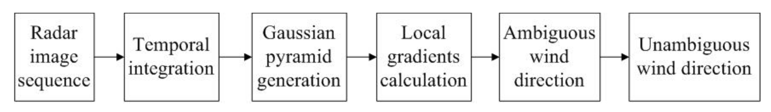
Figure 3.
Flowchart of the optical flow motion estimation-based technique (OFM).
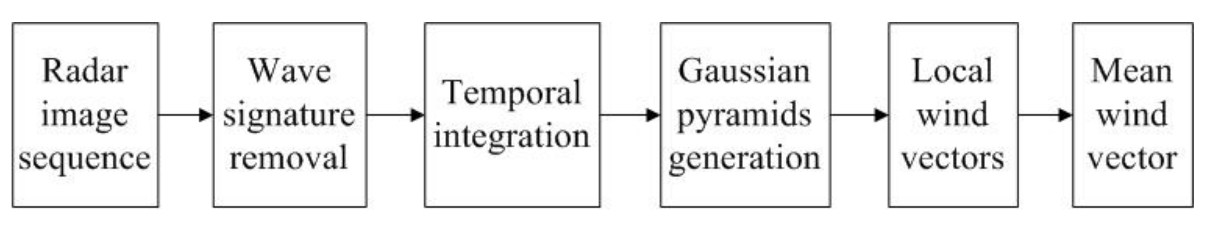
Figure 4.
Basic steps of the single-Curve Fitting (CF) method for wind direction and speed retrieval.
Figure 4.
Basic steps of the single-Curve Fitting (CF) method for wind direction and speed retrieval.

Figure 5.
Basic steps of the original Intensity Level Selection (ILS)-based method for wind parameter estimation.
Figure 5.
Basic steps of the original Intensity Level Selection (ILS)-based method for wind parameter estimation.
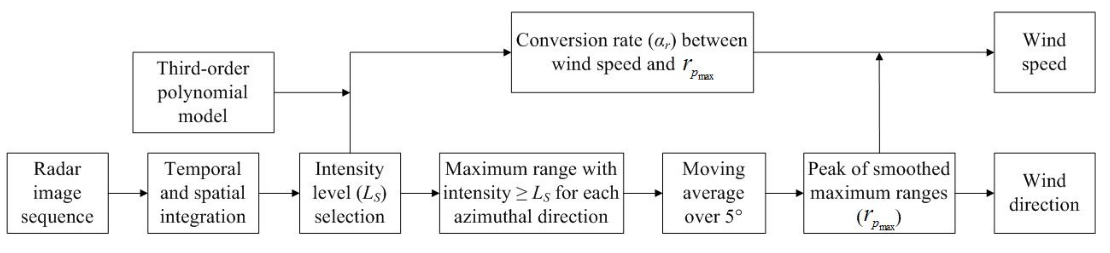
Figure 6.
Basic steps of the ensemble empirical mode decomposition (EEMD)-normalization-based algorithm.
Figure 6.
Basic steps of the ensemble empirical mode decomposition (EEMD)-normalization-based algorithm.
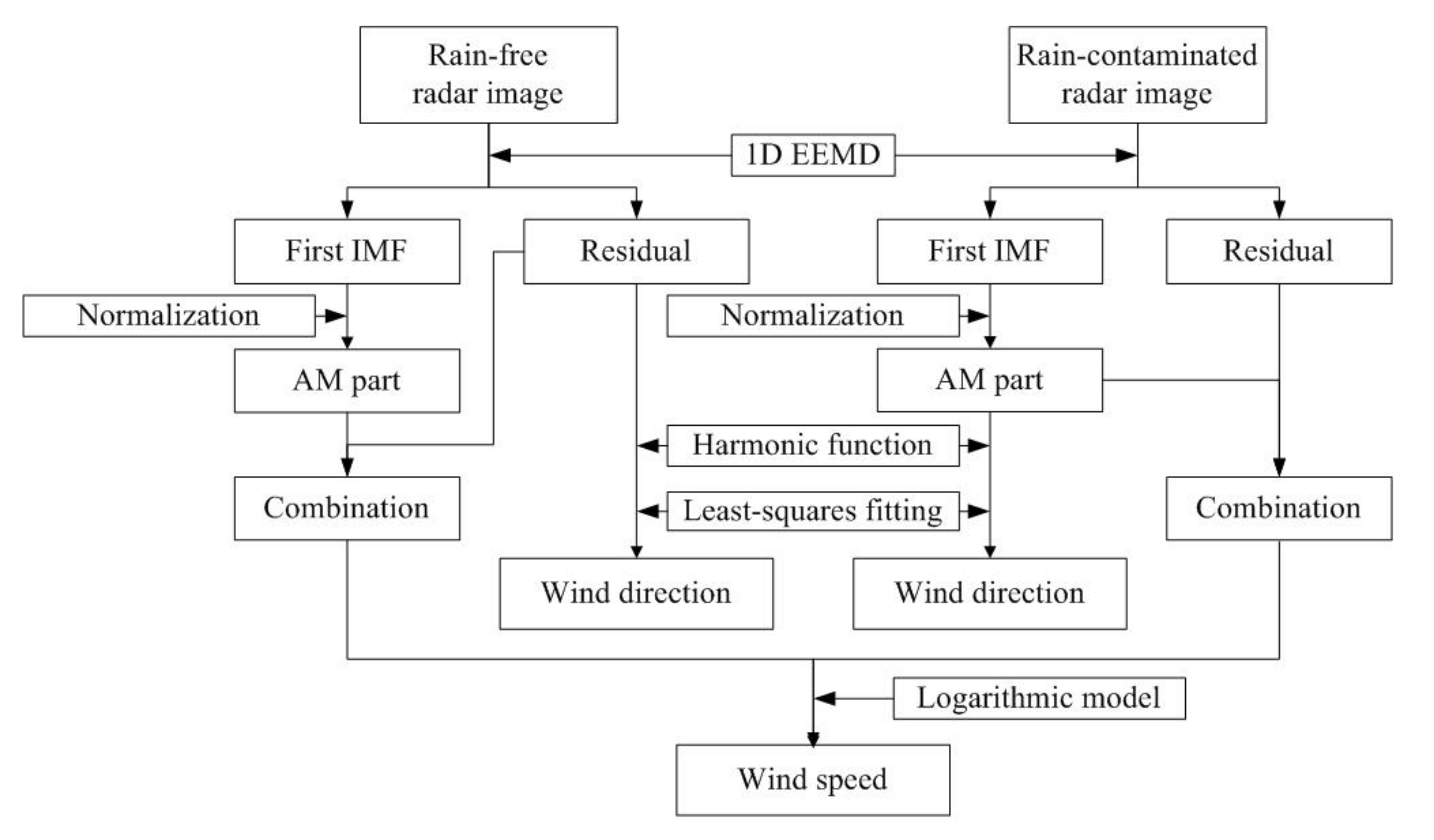
Figure 7.
Basic steps of the traditional 3D discrete Fourier transform (3D-DFT)-based algorithm.
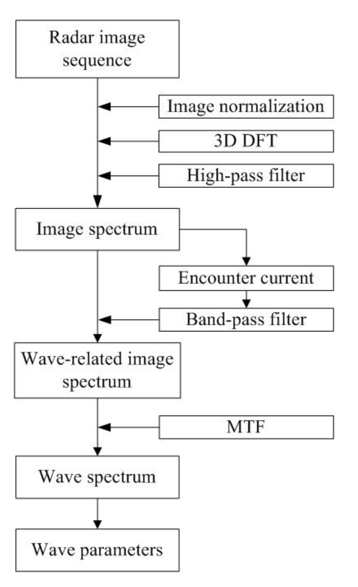
Figure 8.
Flowchart of the adaptive recursive positioning method (ARPM).

Figure 9.
Flowchart of the self-adaptive 2D continuous wavelet transform (2D-CWT)-based algorithm.
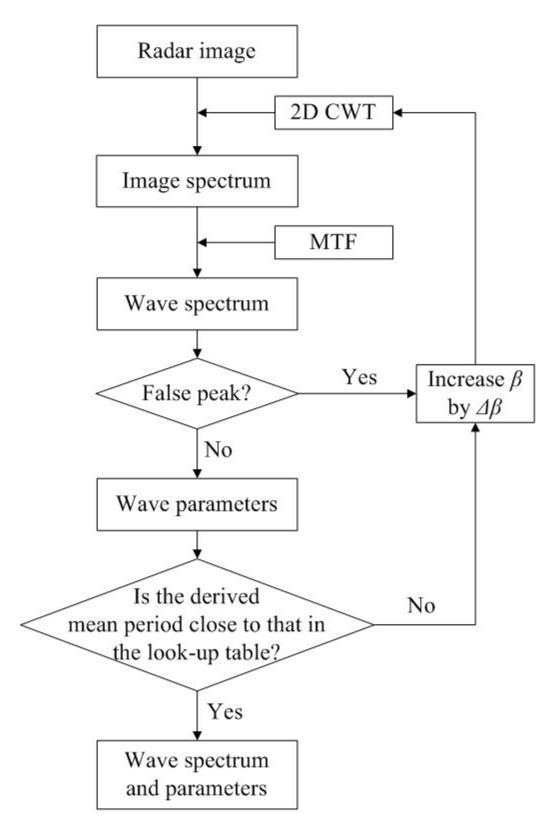
Figure 10.
Basic steps of the array beamforming algorithm.
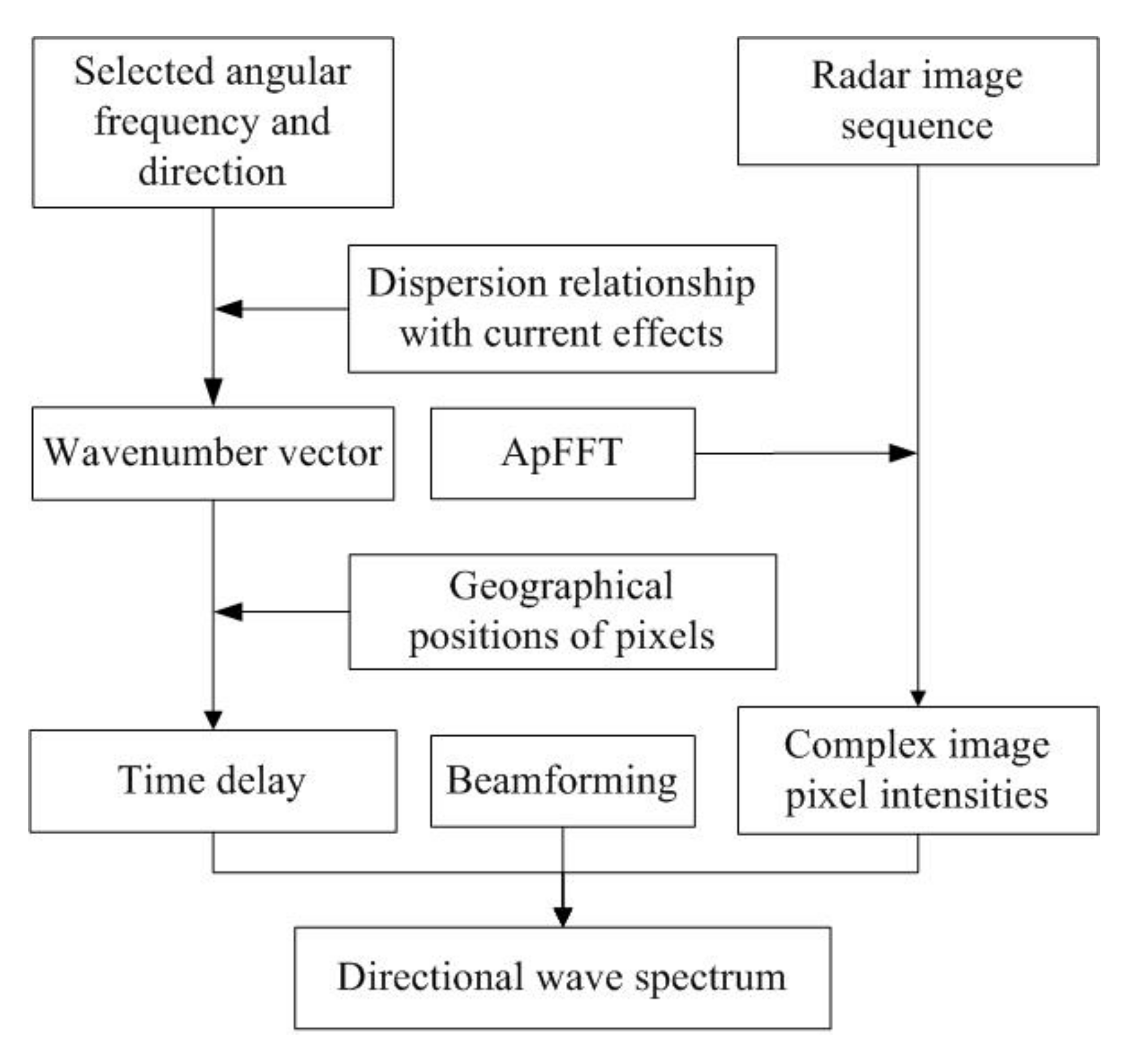
Figure 11.
Basic steps of the shadowing-based algorithm [91].
Figure 11.
Basic steps of the shadowing-based algorithm [91].
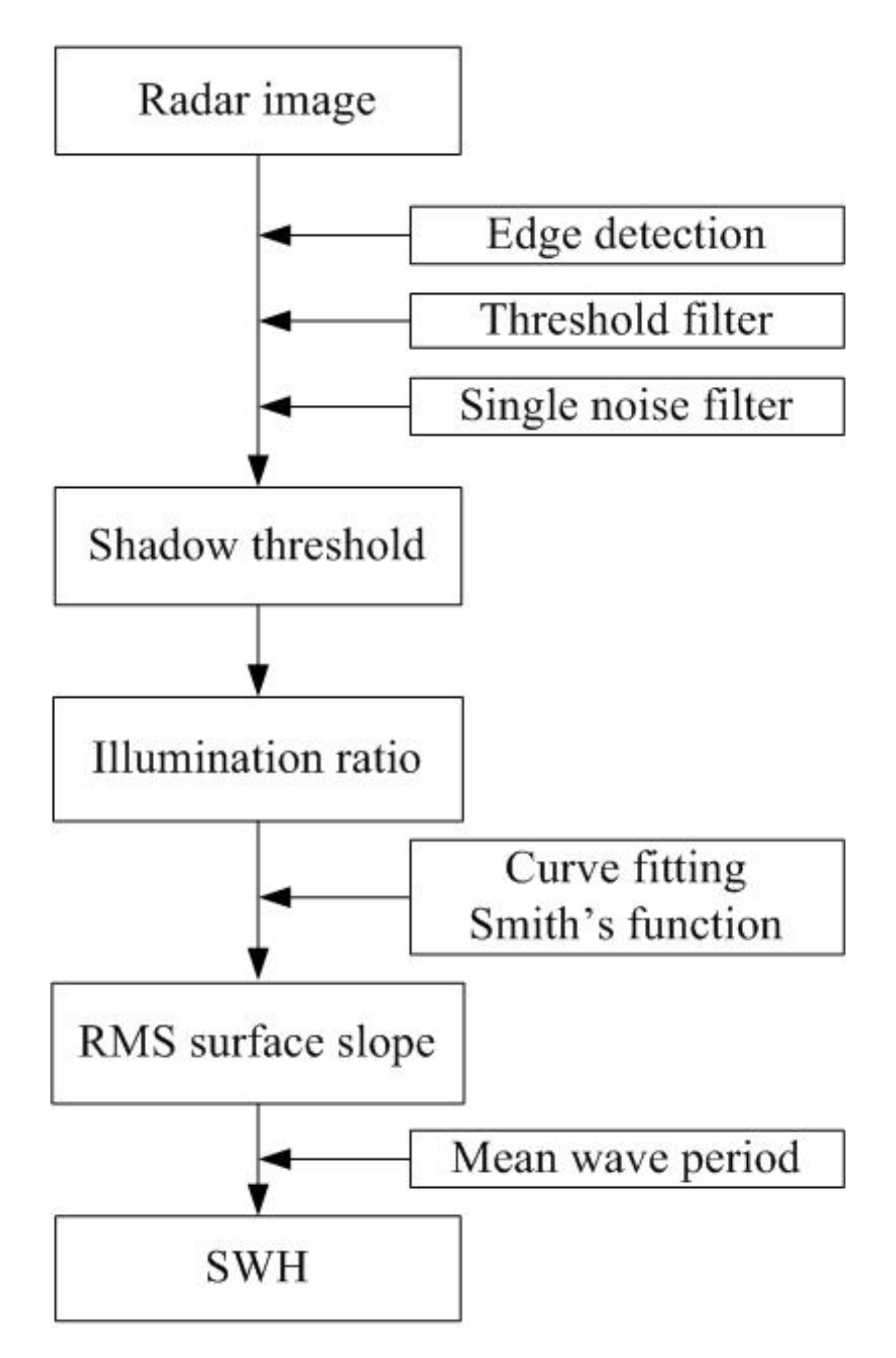
Figure 12.
Basic steps of the empirical orthogonal function (EOF)-principal component (PC)-based algorithm for: (a) and peak wave period; (b) peak wavelength and wave direction.
Figure 12.
Basic steps of the empirical orthogonal function (EOF)-principal component (PC)-based algorithm for: (a) and peak wave period; (b) peak wavelength and wave direction.

Figure 13.
Basic steps of the joint- probability distribution function (PDF)-based algorithm.


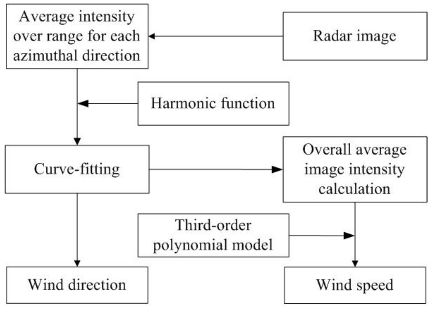
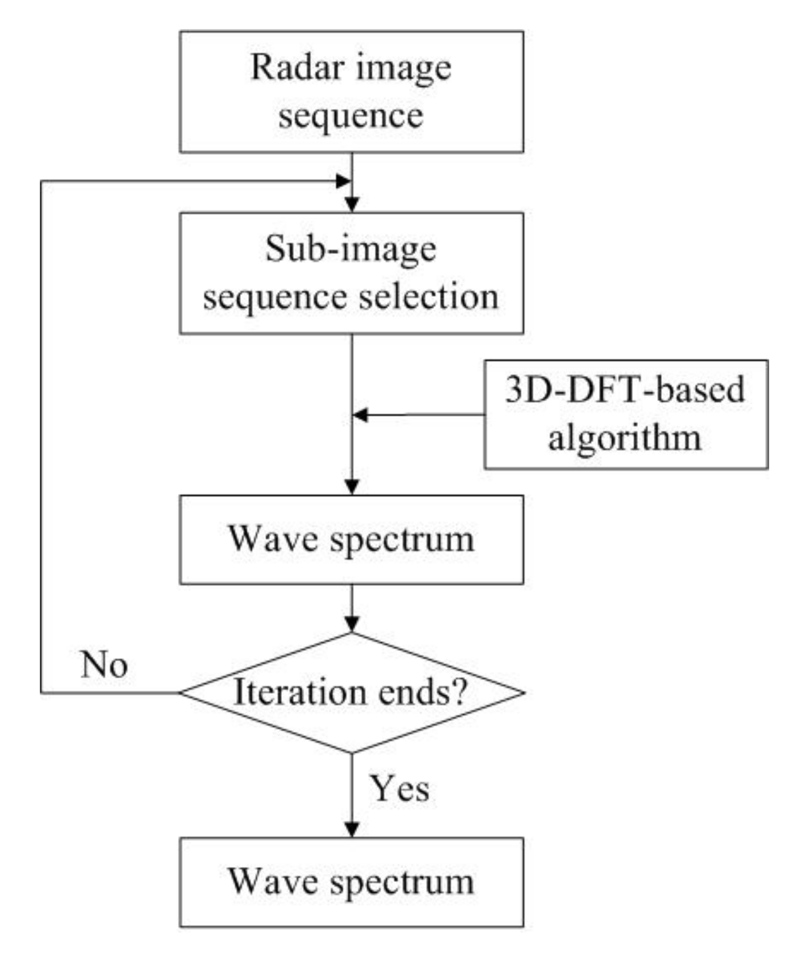
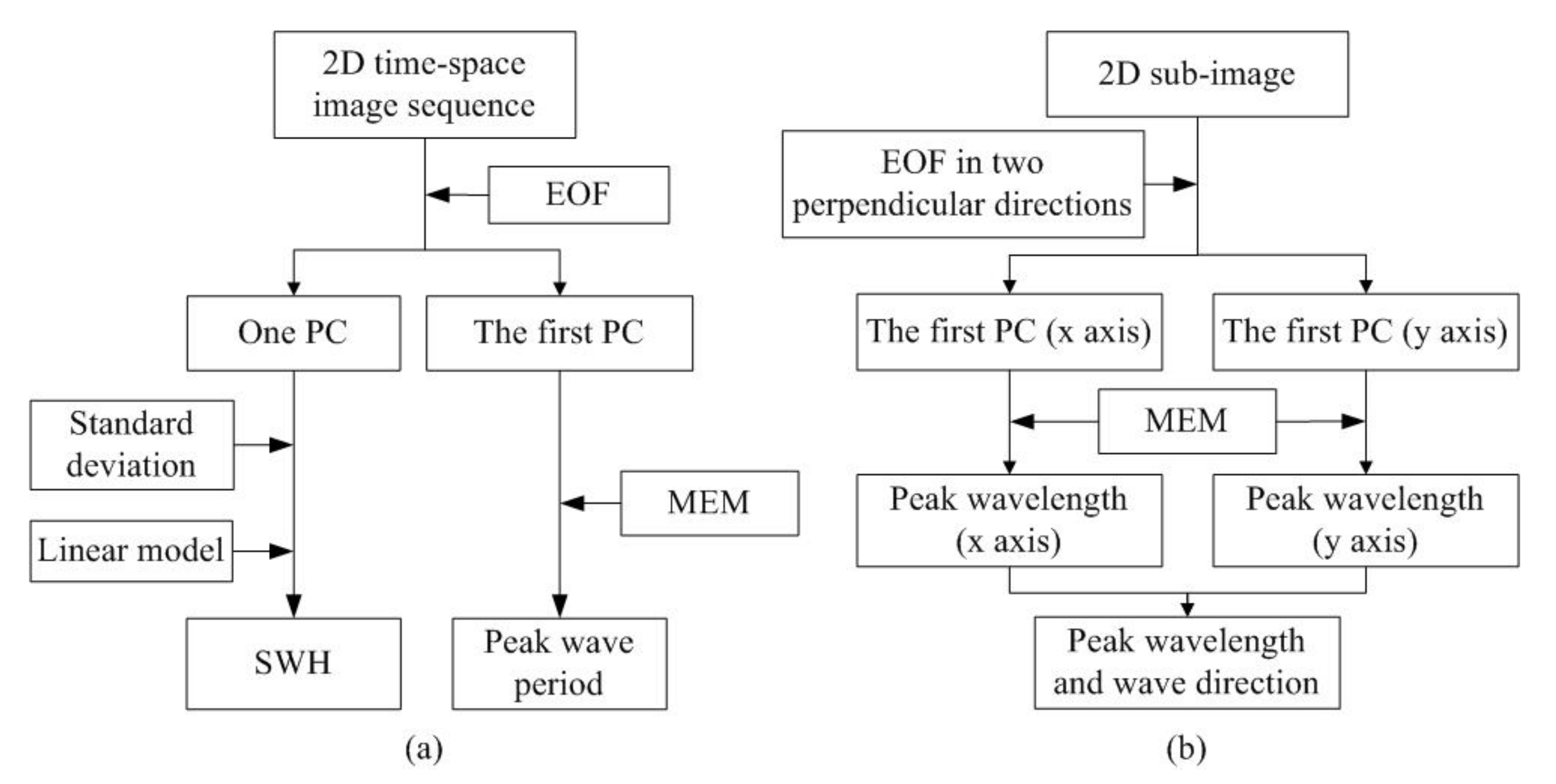
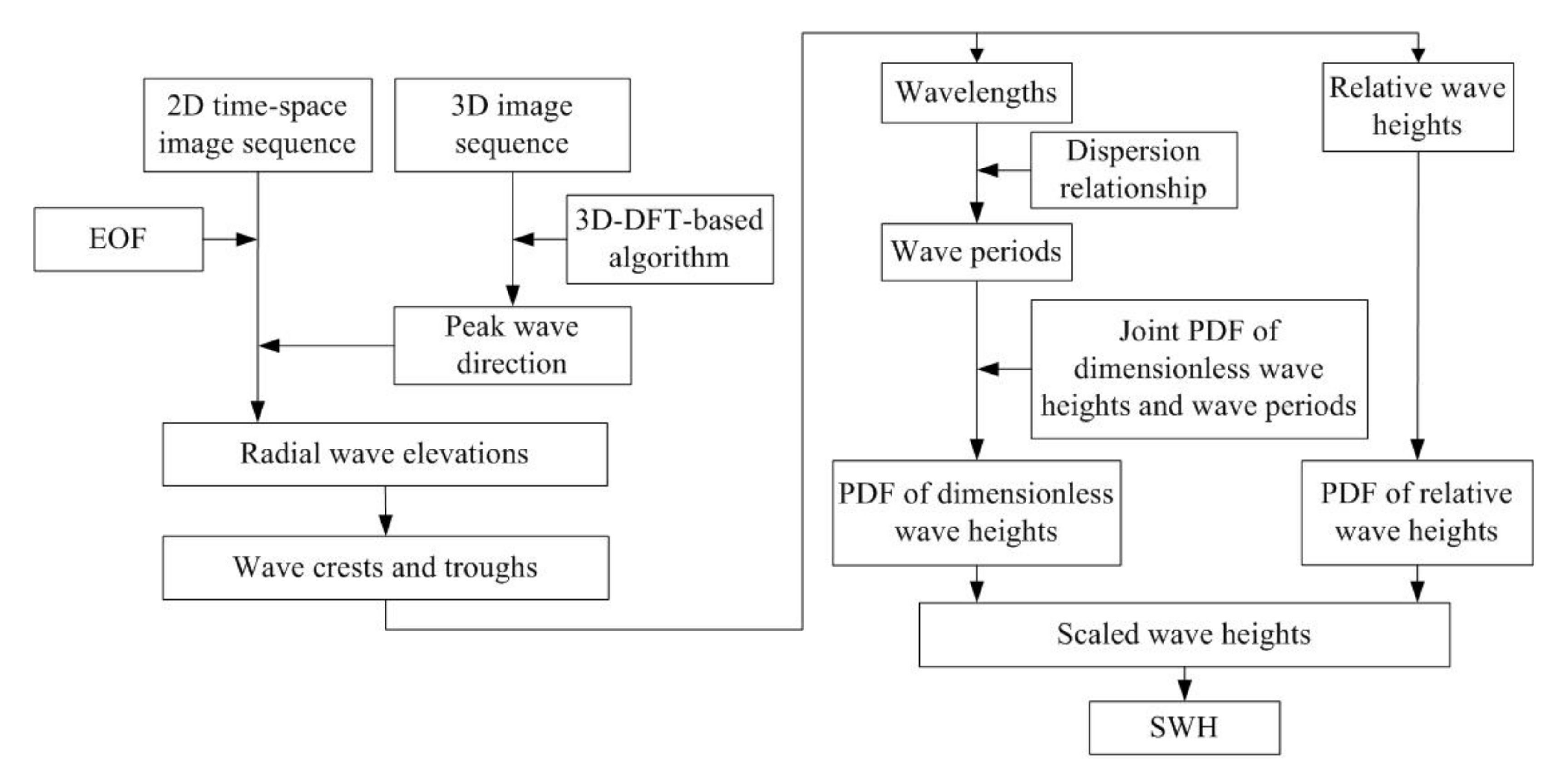
Table 1.
Inter-Comparison of the Reviewed Wind Measurement Techniques.
| Methods | Correlation Coefficient | RMS Difference | Wind Speed Range (m/s) | Applicable Under | Calibration-Free | Images Required | |||||
|---|---|---|---|---|---|---|---|---|---|---|---|
| Wind Direction | Wind Speed | Wind Direction () | Wind Speed (m/s) | Ship Motion | Blockage | Rain | Wind Direction | Wind Speed | |||
| Local Gradients Method & Neural Networks | 0.99 | 0.96–0.99 | 12.8–14.2 | 0.42–0.85 | 0–16/0–18 | × | √ | × | √ | × | Multiple |
| Optical Flow Motion | 0.96 | 0.64 | 32.1 | 2.68 | 0–18 | × | √ | × | √ | √ | Multiple |
| Single Curve Fitting | 0.95–0.97 | 0.90–0.91 | 14.2–17.4 | 0.79–0.88 | 0–15/2–17 | √ | √ | × | √ | × | Single |
| Dual Curve Fitting | - | - | 14.9–16.6 | 1.4–1.9 | 2–16 | √ | √ | × | √ | × | Single |
| Two-Model Curve Fitting | - | - | - | 1.7 | 2–16 | √ | √ | √ | - | × | Single |
| Original Intensity Level Selection | - | - | 11–14.3 | 0.6–0.8 | 4–22 | √ | × | × | √ | × | Multiple |
| Modified Intensity Level Selection | - | - | 11.8–16.3 | 1–1.4 | 2–16 | √ | √ | × | √ | × | Multiple |
| Texture-Analysis -Incorporated | - | - | 16.8 | 1.5 | 2–16 | √ | √ | √ | √ | × | Multiple |
| Probability Distribution Function | - | - | 26.2 | 1.37 | 0–20 | √ | √ | × | × | × | Single |
| Background Noise | - | 0.89 | - | 2.86 | 1–10 | √ | × | × | - | × | Multiple |
| 1D Spectral Analysis | - | 0.89 | 15.8 | 1.6 | 2–16 | √ | √ | √ | √ | × | Single |
| 1D/2D Ensemble Empirical Mode Decomposition | 0.98 | - | 11.4–12.7 | - | - | √ | √ | √ | √ | − | Single |
| Ensemble Empirical Mode Decomposition - Normalization | - | - | 11.5 | 1.31 | 2–16 | √ | √ | √ | √ | × | Single |
Table 2.
Inter-Comparison of the Reviewed Wave Measurement Techniques.
| Methods | Wave Spectrum Estimation | Wave Height Measurement | Correlation Coefficient of | RMS Difference of (m) | Range of (m) | Calibration - Free | Images Required |
|---|---|---|---|---|---|---|---|
| Traditional 3D DFT | √ | √ | 0.71–0.89 | 0.18–0.42 | 0.5–2/ 1–4/ 0.5–5.5 | × | Multiple |
| Multilayer Perceptrons | √ | √ | 0.96–0.97 | 0.22–0.27 | 0.5–8/ 0.5–10 | × | Multiple |
| Iterative Least-Squares | √ | × | - | - | - | × | Multiple |
| Quadratic Polynomial MTF | √ | × | - | - | - | × | Multiple |
| Variable-Exponent Linear MTF | √ | × | - | - | - | × | Multiple |
| Adaptive Recursive Positioning | √ | × | - | - | - | × | Multiple |
| Geometrics-Based SNR Estimation | √ | √ | 0.89 | 0.19 | 0.5–2 | × | Multiple |
| 2D Continuous Wavelet Transform | √ | √ | - | 0.61 | 2–3.5 | × | Single |
| Array Beamforming | √ | √ | 0.95 | 0.12 | 0.5–2 | × | Multiple |
| Illumination Probability | × | √ | 0.54–0.67 | - | 1–6.5 | × | Single |
| Statistical Analysis | × | √ | 0.65–0.67 | 0.68–0.77 | 0.5–9 | × | Single |
| Tilt-Based | × | √ | 0.94 | 0.35 | 0.5–6 | √ | Multiple |
| Original Shadowing-Based | × | √ | 0.87 | - | 1.5–10.5 | √ | Single |
| Modified Shadowing-Based | × | √ | 0.81 | 0.47 | 1–5 | √ | Single |
| Water-Depth-incorporated | × | √ | 0.68 | 0.51 | 0.5–5 | √ | Single |
| Support Vector Regression | × | √ | - | 0.38–0.82 | 2–6/ 2–9 | √ | Single |
| Empirical Orthogonal Function-Principal Component | × | √ | 0.93 | 0.21 | 0.5–3.5 | × | Multiple |
| Rotated Empirical Orthogonal Function | × | √ | 0.88–0.92 | 0.14–0.17 | 0.5–1.8 | × | Multiple |
| Empirical Orthogonal Function-Joint PDF | × | √ | 0.77–0.78 | 0.51 | 0.2–3.5 | √ | Multiple |
| Ensemble Empirical Mode Decomposition | × | √ | 0.91 | 0.36 | 1–5 | × | Single |
| Coherent radar | √ | √ | 0.98 | 0.15–0.23 | 0–5 | √ | Multiple |
© 2017 by the authors. Licensee MDPI, Basel, Switzerland. This article is an open access article distributed under the terms and conditions of the Creative Commons Attribution (CC BY) license (http://creativecommons.org/licenses/by/4.0/).
Share and Cite
MDPI and ACS Style
Huang, W.; Liu, X.; Gill, E.W. Ocean Wind and Wave Measurements Using X-Band Marine Radar: A Comprehensive Review. Remote Sens. 2017, 9, 1261. https://doi.org/10.3390/rs9121261
AMA Style
Huang W, Liu X, Gill EW. Ocean Wind and Wave Measurements Using X-Band Marine Radar: A Comprehensive Review. Remote Sensing. 2017; 9(12):1261. https://doi.org/10.3390/rs9121261
Chicago/Turabian StyleHuang, Weimin, Xinlong Liu, and Eric W. Gill. 2017. "Ocean Wind and Wave Measurements Using X-Band Marine Radar: A Comprehensive Review" Remote Sensing 9, no. 12: 1261. https://doi.org/10.3390/rs9121261
Note that from the first issue of 2016, this journal uses article numbers instead of page numbers. See further details here.