A Novel Pixel-Level Image Matching Method for Mars Express HRSC Linear Pushbroom Imagery Using Approximate Orthophotos

1
Department of Aerial Photogrammetry, Xi’an Information Technique Institute of Surveying and Mapping, Xi’an 710054, China
2
Department of Photogrammetry, Zhengzhou Institute of Surveying and Mapping, Zhengzhou 450052, China
*
Author to whom correspondence should be addressed.
Remote Sens. 2017, 9(12), 1262; https://doi.org/10.3390/rs9121262
Submission received: 25 October 2017
/
Revised: 1 December 2017
/
Accepted: 2 December 2017
/
Published: 5 December 2017
(This article belongs to the Section Remote Sensing Image Processing)
Abstract
:Mars topographic data, such as digital orthophoto maps (DOMs) and digital elevation models (DEMs) are essential to planetary science and exploration missions. The main objective of our study is to generate a higher resolution DEM using the Mars Express (MEX) High Resolution Stereo Camera (HRSC). This paper presents a novel pixel-level image matching method for HRSC linear pushbroom imagery. We suggest that image matching firstly be carried out on the approximate orthophotos. Then, the matched points are converted to the original images for forward intersection. The proposed method adopts some practical strategies such as hierarchical image matching and normalized cross-correlation (NCC). The characteristic strategies are: (1) the generation of a DEM and a DOM at each pyramid level; (2) the use of the generated DEM at the current pyramid level as reference data to generate approximate orthophotos at the next pyramid level; and (3) the use of the ground point coordinates of orthophotos to estimate the approximate positions of conjugate points. Hence, the refined DEM is used in the image rectification process, and pixel coordinate displacements of conjugate points on the approximate orthophotos will become smaller and smaller. Four experimental datasets acquired by the HRSC were used to verify the proposed method. The generated DEM was compared with the HRSC Level-4 DEM product. Experimental results demonstrate that an accurate and precise Mars DEM can be generated with the proposed method. The approximate positions of the conjugate points can be estimated with an accuracy of three pixels at the original image resolution level. Though slight systematic errors of about two pixels were observed, the generated DEM results show good consistency with the HRSC Level-4 DEM.
1. Introduction
Mars, the fourth planet from the Sun, is the first choice for deep space exploration missions. Since the 1970s, humans have launched many orbiters and rovers to the red planet [1,2,3,4,5,6]. Mars mapping is essential to planetary exploration missions, which require landing site selection, hazard avoidance, and rover navigation. Additionally, topographic maps of Mars are widely used in planetary sciences such as geomorphology, geology, and mineralogy [7,8]. Mars topographic data can be derived through the photogrammetric processing of orbital stereo photographs. Both open source and commercial software are widely used in the planetary mapping community. Integrated Software for Imagers and Spectrometers (ISIS) developed by the United States Geological Survey (USGS) Astrogeology Team and Ames Stereo Pipeline (ASP) developed by the National Aeronautics and Space Administration (NASA) Ames Research Center are types of open source software [9,10]. ISIS and ASP facilitate the photogrammetric processing of planetary imagery greatly. Commercial photogrammetric software such as the Socet Set from BAE Systems (Farnborough, UK) has also been used in several planetary exploration missions to generate planetary topographic maps [2,3,4,11,12].
The photogrammetric processing techniques applied in Mars mapping have been presented comprehensively in the literature [1,2,3,4,5,6,9,10,11,12,13,14,15,16,17,18,19,20]. The Viking orbiter images were acquired in the 1970s, and were used to generate many valuable Mars topographic maps in the early days [1]. After the Mars Orbiter Laser Altimeter (MOLA), the digital elevation model (DEM) became available. The Viking Orbiter stereo models were controlled by MOLA DEM to improve absolute accuracy [13]. Kirk et al. generated a high-resolution digital elevation model (DEM) using Mars Global Surveyor (MGS) Mars Orbiter Camera (MOC) narrow angle images to access the safety of candidate landing sites for the Mars Exploration Rovers (MERs) [3]. Shan et al. performed a photogrammetric analysis of MGS mapping data, and proposed a method to register the MOLA profiles to MOC images [14]. Scholten et al. introduced the High Resolution Stereo Camera (HRSC) data processing methods and operational aspects, including data calibration, bundle adjustment, DEM and orthophoto generation [12]. Kirk et al. reported that very high resolution topographic data could be generated from the Mars Reconnaissance Orbiter (MRO) High Resolution Imaging Science Experiment (HiRISE) stereo images, and meter-scale slopes of candidate Phoenix landing sites were derived [4]. Li et al. developed a rigorous photogrammetric model for HiRISE stereo image processing, using third-order polynomials to model the change in exterior orientation (EO) parameters over time [15]. A detailed review of Mars mapping is out of the scope of this paper, though a recent review has been presented by Wu [6].
Several Mars exploration missions have been carried out, with one of the main objectives being Mars mapping, for example Viking in the 1970s [1,13], MGS in the 1990s [3,14], and Mars Express (MEX) [11,12] and MRO [4,15] after the year 2000. HiRISE on MRO provides the highest image resolution of Mars, which is up to 25 cm per pixel [4]. The image resolution of MGS MOC narrow angle camera (NAC) ranged from 1.5 m to 12 m. Though HiRISE and MOC NAC obtained high resolution images, the stereo photographs acquired by these cameras covered only a small portion of the entire Martian surface [3]. Compared to other terrain mapping cameras, HRSC has the advantages of having global coverage, high image resolution, and multi-stereo capabilities. Currently, photographs acquired by HRSC have almost covered the entire Martian surface. Thus, orbital photographs acquired by HRSC are the best data sources for the generation of global Mars topographic maps. The HRSC team and many researchers investigated the photogrammetric processing of HRSC stereo photographs [16,17,18,19,20]. The early released HRSC Level-4 products were generated using single orbit data. Recently, new global mapping program using the complete HRSC mission data was performed by the HRSC team, and multi-orbit DEM products were derived [19]. The grid spacing of the recent multi-orbit DEM products was about 50 m, which was still 2~3 times larger than the original image resolution. It is expected that a higher resolution Mars global DEM can be generated using the pixel-level image matching method. Moreover, future Mars exploration missions will put greater emphasis on science return, and require higher resolution Mars topographic maps to ensure safe landing and traverse.
Image matching is a classical problem in photogrammetry and computer vision [21], and can be used to generate DEM automatically [22,23,24]. In recent years, several dense image matching methods such as geometrically constrained cross-correlation (GC3) algorithm [25], semi-global matching (SGM) [26], patch-based multi-view stereo matching (PMVS) [27] and SURE [28] have been proposed. However, these methods were primarily designed for earth observation images, and require substantial optimization when used for Mars orbital photographs. Kirk et al. presented DEM results derived from HiRISE stereo images using Automatic Terrain Extraction (ATE) and Next-Generation ATE (NGATE) modules provided by Socet Set [4], and pointed out that matching strategy parameters were essential for generating Mars DEM. Due to the special terrain characteristics of the Martian surface such as low contrast, traditional image matching methods may fail or deliver poor results for Mars orbital photographs. Therefore, it is very meaningful to develop a targeted image matching method for Mars mapping. The HRSC team determined the conjugate points using quasi-epipolar geometry and area-based multi-image matching [12]. The SGM method was also used to process HRSC linear pushbroom imagery, which requires that the original stereo images firstly undergo epipolar resampling [16]. Additionally, Shape from Shading (SfS) is also utilized to refine the DEM generated by stereo photogrammetry [29].
In this paper, we propose a novel pixel-level image matching method for HRSC linear pushbroom imagery, with the main objective of generating a higher resolution Mars DEM. The remainder of this paper is organized as follows. The proposed pixel-level image matching method is discussed in Section 2. The experimental results and detailed analysis are presented in Section 3. Section 4 presents discussion. Section 5 concludes this paper by discussing the pros and cons of the proposed method and the possible improvements.
2. Materials and Methods
2.1. Terrain Characteristics of the Martian Surface
Traditional image matching methods are mainly designed for earth observation images, which may not be suitable for the Martian surface. The main disadvantages of Martian surface image matching are summarized as follows.
- (1)
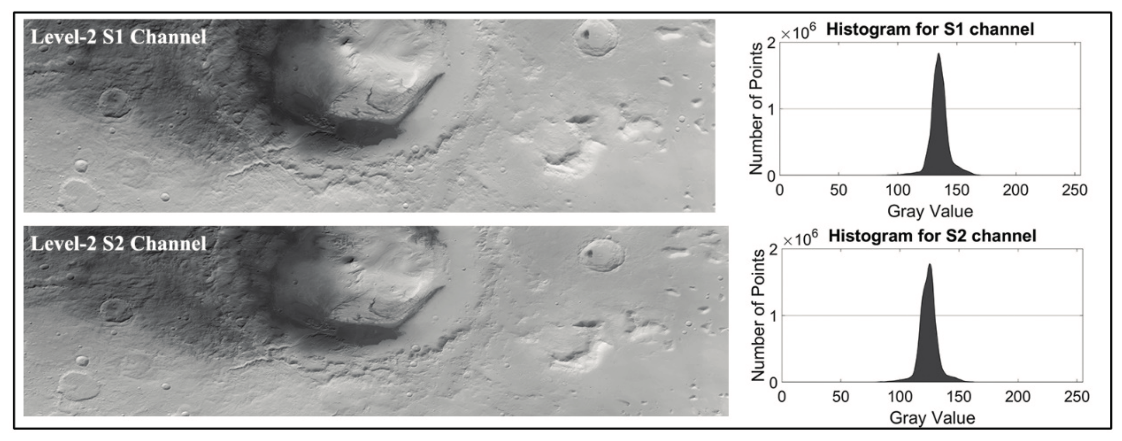
- Low contrast. As observed in the left parts of Figure 1, Martian surface images always deliver low contrast compared with the rich texture information delivered by images of earth. The right parts of Figure 1 show that the histograms concentrate in a small range. Thus, the low signal-to-noise ratio of Martian surface images will decrease the success rate of image matching.
- (2)
- Insufficient feature points. Feature-based matching methods such as scale-invariant feature transform (SIFT) and speeded up robust features (SURF) are more robust than area-based matching methods. Unfortunately, the feature points on Martian surface images are very limited. These feature points can be used as tie points for bundle adjustment, which are not suitable for generating DEM.
- (3)
- Poor image quality. Image quality is influenced by many factors such as imaging instruments, atmospheric environment, incidence angle and emission angle. It is well known that Martian surface images perform worse than earth observation images as far as image quality is concerned.
- (4)
- Repetitive patterns. Repetitive patterns will result in wrongly matched points especially when an area-based matching method is carried out. To address this issue, some constraint conditions such as camera geometry need to be utilized.
On the other hand, when compared to earth observation images, Martian surface images exhibit some advantages for image matching: (1) there are no trees or rivers on the Martian surface; (2) it is also impossible for moving objects such as cars to appear on Martian surface; and (3) occlusions caused by high buildings and tall trees on earth observation images can be avoided. In short, in terms of terrain continuity, Martian surface images perform better than earth observation images. Thus, the proposed image matching method will make full use of the terrain characteristics of the Martian surface.
2.2. Image Geometry of HRSC
The image geometry of the HRSC imaging instrument is essential to the proposed pixel-level image matching method. In order to perform image matching on the approximate orthophotos and generate high-resolution DEM products, the coordinates transformation between the original HRSC Level-2 images and the approximate orthophotos must be established.
2.2.1. HRSC Linear Pushbroom Imagery Overview
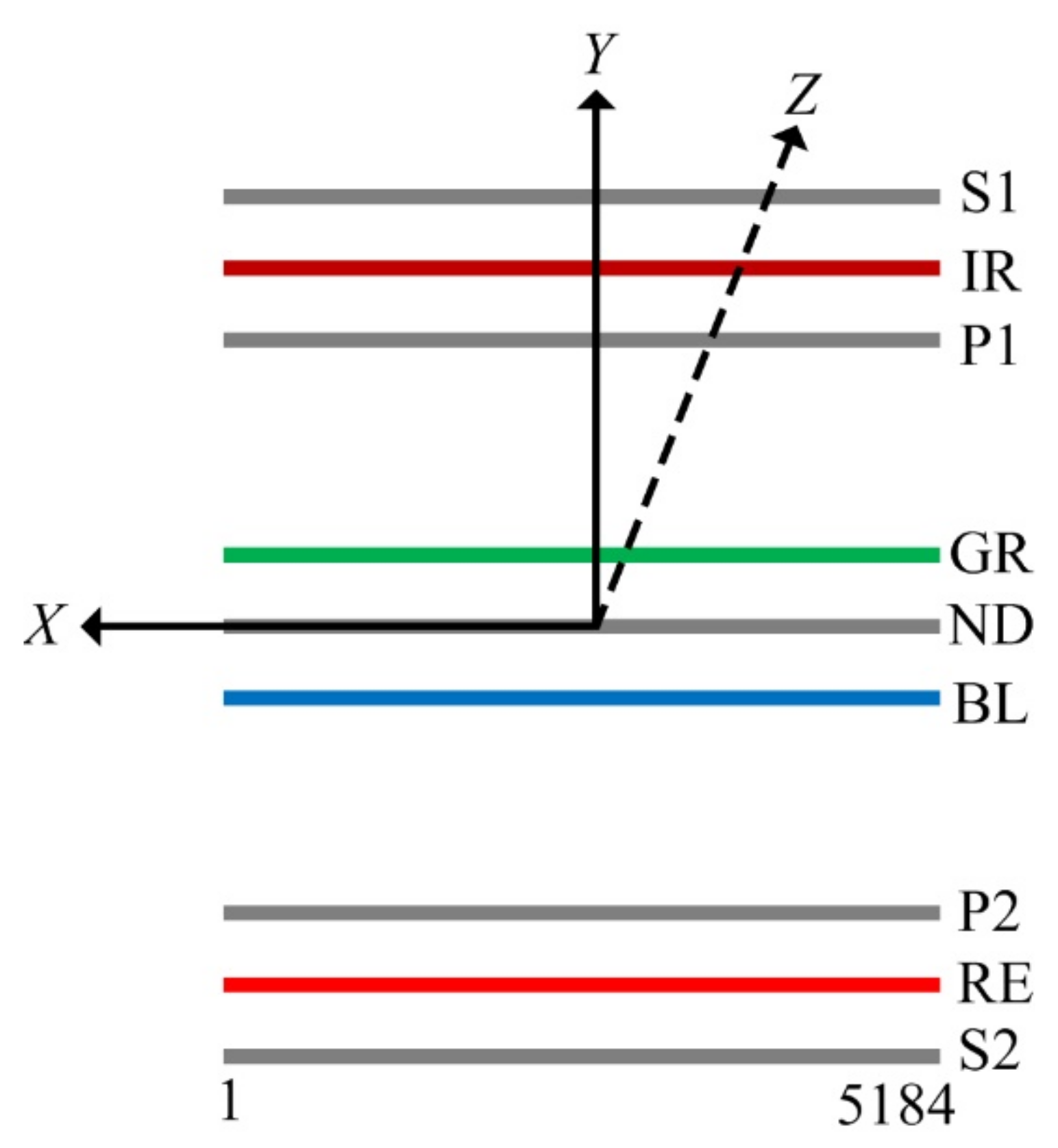
MEX was launched in June 2003, and entered Mars on 25 December 2003. The HRSC, carried on the MEX, has been imaging the Martian surface since January 2004, and is, to date, still operational. At an altitude of 250 km, the maximum image resolution of HRSC imagery is about 10 m per pixel. As described in Figure 2, HRSC is a linear camera with five panchromatic channels and four color channels, which can acquire stereoscopic photographs in a single orbit. Nine charge-coupled device (CCD) linear arrays were mounted in parallel in the focal plane, and each scan line has 5184 pixels with a pixel size of 7 μm [11,12].
The HRSC can provide high-resolution multi stereo and multi spectral images, and was specially designed by German Aerospace Center (DLR) for Mars mapping. The nominal focal length of HRSC is 175 mm for all linear arrays. However, in order to generate precise topographic data, more accurate on-orbit geometric calibration results must be used. Table 1 lists the calibrated camera geometric parameters such as focal length and boresight sample extracted from Spacecraft, Planet, Instrument, C-Matrix, Events (SPICE) kernels [30]. The following affine transformation equations are used to convert CCD pixel coordinates (Line, Sample) to image point coordinates (x, y).
where the affine transformation coefficients and can be acquired from the related SPICE kernels.
The emphasis time (ET) is used to extract the EO parameters for each scan line. The line exposure duration (LED) of HRSC imagery varies within a strip. Taking orbit 5273 as an example, Table 2 lists the LED for the S1 channel. The LED parameters are used to construct the rigorous geometric model for HRSC linear pushbroom imagery, and can be extracted with ISIS’s tabledump program.
2.2.2. Rigorous Geometric Model
The rigorous geometric model is essential to the photogrammetric processing of linear pushbroom imagery. It is the foundation for coordinate transformation between the image point and ground point. In theory, due to the pushbroom imaging principle of linear cameras, each scan line of HRSC imagery has six EO parameters. The central projection holds true for each scan line. The rigorous geometric model for HRSC linear pushbroom imagery is established with the extended collinearity equation.
where are 2D image point coordinates, is focal length, are 3D ground point coordinates, represents the scan line, (, , ), and are the position component and rotation matrix elements of EO, respectively. The unit of 2D image point coordinates and 3D ground point coordinates is meters. In order to construct Equation (2), the following data must be provided: (1) each scan line’s exposure time; (2) each scan line’s EO parameters; and (3) each sample’s image point coordinates. Given an image point p with CCD pixel coordinates , the accurate exposure time for scan line l is calculated using the extracted LED parameters. Then, the EO parameters for scan line l are acquired by invoking the SPICE kernels. The image point coordinates of image point p are calculated with Equation (1). We use the following SPICE function to acquire the pointing data of MEX HRSC imagery.
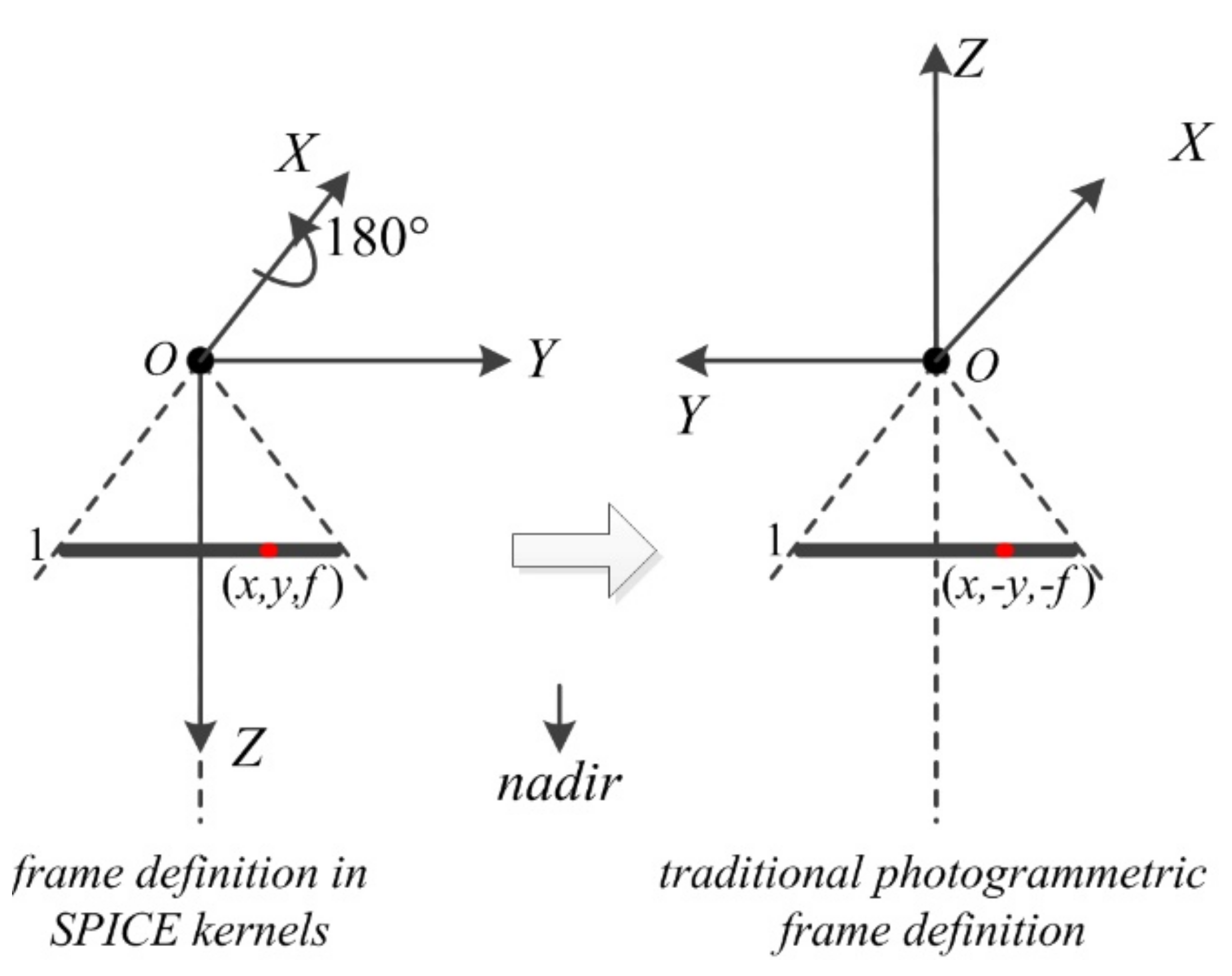
where “MEX_HRSC_HEAD” and “IAU_MARS” represents the MEX HRSC frame and body-fixed Martian Cartesian coordinate frame respectively, ET represents emphasis time and RM is used to store the rotation matrix between “MEX_HRSC_HEAD” and “IAU_MARS”. However, the frame definition acquired from SPICE kernels is different from the traditional photogrammetric frame definition. As observed in the left part of Figure 3, the Z axis of the MEX HRSC frame acquired from SPICE kernels points toward the Martian surface. In contrast, in the traditional photogrammetric frame, the Z axis points upwards. For ease of calculation, we convert the SPICE frame definition to the traditional photogrammetric frame definition by rotating 180 degrees around the X axis (See Figure 3). Consequently, the original image space coordinates are converted to .
pxform_c (“MEX_HRSC_HEAD”, “IAU_MARS”, ET, RM);
2.2.3. Fast Back-Projection Algorithm
In photogrammetric processing procedures such as geometric rectification, coordinate transformation from a 3D ground point to a 2D image point, namely back-projection, is required. Meanwhile, back-projection is also a critical step for the proposed image matching method, which is used to convert the matched points from the approximate orthophotos to the original images. Unfortunately, though Equation (2) establishes the coordinates transformation between the image points and the ground points, the exact scan line corresponding to a ground point is not known in advance. Therefore, for linear pushbroom imagery, in order to perform back-projection the exact scan line corresponding to a ground point must be determined first.
The back-projection algorithm was implemented in ISIS and SPICE to support many planetary exploration missions such as MGS and MRO. The software tool cam2map provided in ISIS was used to generate orthophotos from original planetary images [9]. A back-projection algorithm was also implemented in the automated cloud tracking system for the Akatsuki Venus Climate Orbiter data [31]. Many researchers noted the importance of back-projection for photogrammetric processing of linear pushbroom imagery, and several back-projection algorithms were presented [32,33,34,35]. The proposed algorithms for back-projection can be divided into either image space iteration (ISI) or object space iteration (OSI). The ISI algorithm is characterized by iterative computation in image space, which requires complicated computation using the collinearity equation. In contrast, the OSI algorithm uses the geometric constraints in object space to determine the exact scan line, which outperforms ISI. The OSI algorithm was proposed by Wang et al. [33], and was specially designed for airborne linear pushbroom images. Using the basic scheme of OSI algorithm, we carry out further algorithm optimization according to the HRSC image geometry. We note that for HRSC pushbroom imagery, all pixels of a certain channel are along a straight line. Thus, there is no need to carry out segmentation for the linear arrays of HRSC, which is required for airborne linear cameras such as ADS40 [33,35]. Additionally, the exact EO corresponding to the ground point is interpolated with linear interpolation using two adjacent scan lines’ EO to achieve sub-pixel accuracy. Moreover, the distance between two adjacent projection planes can be used to predict the exact scan line. Due to the fact that we perform pixel-level image matching, the determined scan line can be used as a good guide for subsequent points.
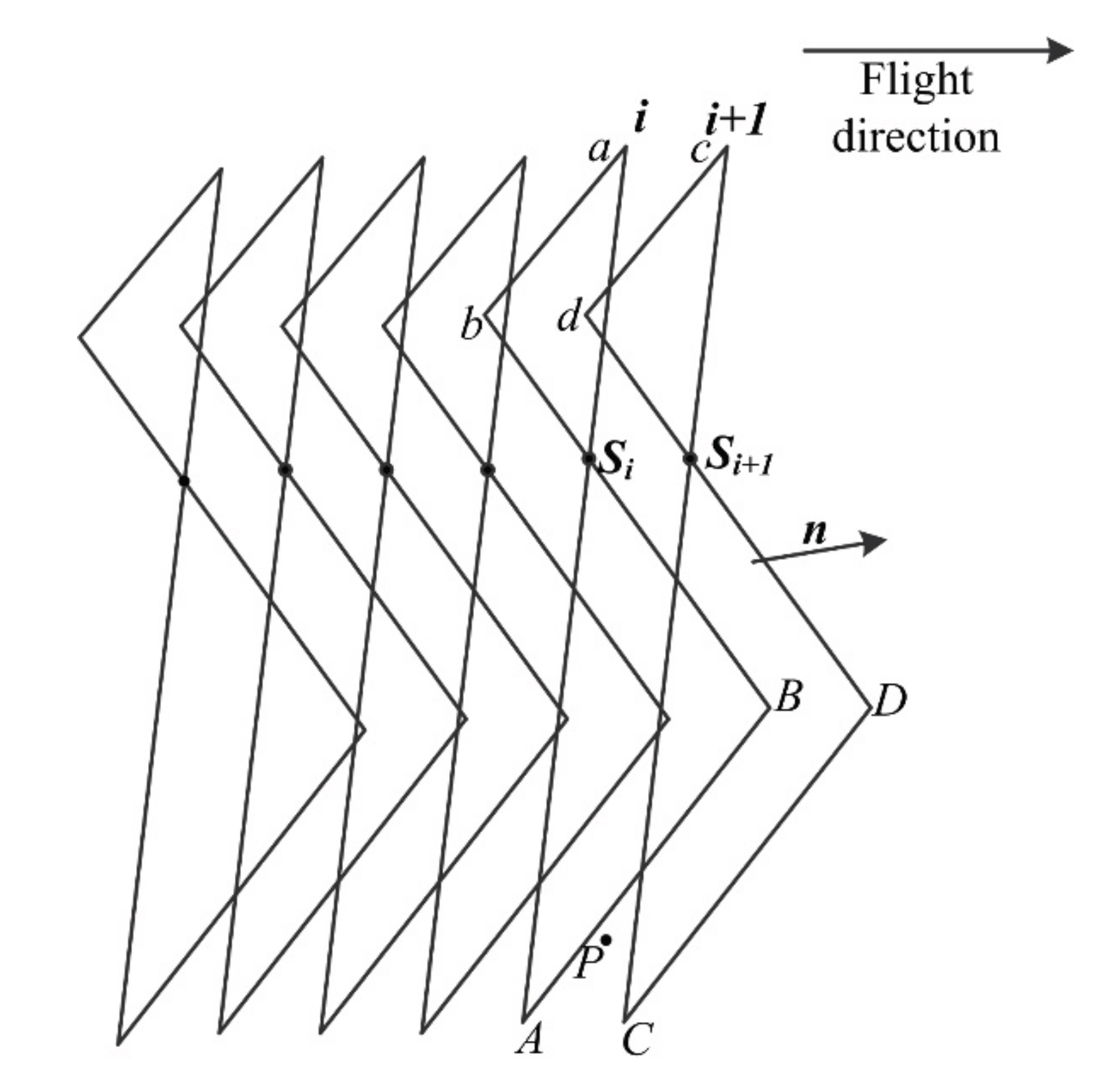
Figure 4 illustrates the basic principle of the fast back-projection algorithm. Suppose ab and cd are the image points of the two adjacent scan lines and , respectively, and are the corresponding ground points, and and are the corresponding exposure stations. The projection plane corresponding to scan line can be determined using the ground points , and This projection plane is referred to as . Firstly, we give the general plane equation in 3D object space.
where , , and are constants to describe the plane equation, and () are the 3D ground point coordinates on the plane. The four constants in Equation (3) can be determined using three ground points on the plane, and the detailed method is described as follows. Given three ground points , and on an identical plane, the following mathematical equation is constructed.
Thus, through simple mathematical calculation, the four constants in Equation (3) can be determined.
Consequently, the distance between the ground point P and the projection plane is calculated using the following equation.
where , , are the object coordinates of ground point P. Obviously, the computation cost using Equation (5) is quite small compared with the complicated collinearity equation. Hence through several fast iterations in object space, the exact scan line for the ground point can be determined.
The experiment was carried out to evaluate the performance of the fast back-projection algorithm. HRSC S1 and S2 channel images are used. We compared the computation efficiency between the traditional ISI algorithm and the fast back-projection algorithm. The tests were performed with Intel Core i5 CPU and 8 GB RAM capacity. We use 1 million ground points to perform the back-projection operation. The back-projected image points’ coordinates were compared with the known ones, and the maximum errors were calculated. The computation times (CTs) were measured as well. The experimental results are given in Table 3. It is observed that the computation efficiency of the fast back-projection algorithm can achieve about 1 million points per second. The fast back-projection algorithm is about 20 times faster than the traditional ISI algorithm. Moreover, the test results shown in Table 3 were acquired with single-threaded programming. Hence more performance gains can be obtained using multithreaded programming. Therefore, the fast back-projection algorithm for HRSC linear pushbroom imagery can meet the proposed image matching method very well.
2.3. Pixel-Level Image Matching Strategies
In this subsection, the proposed pixel-level image matching method for HRSC linear pushbroom imagery is described in detail. The basic principle of the proposed method is presented in Figure 5. The main image matching strategies of the proposed method can be summarized as follows.
- (1)
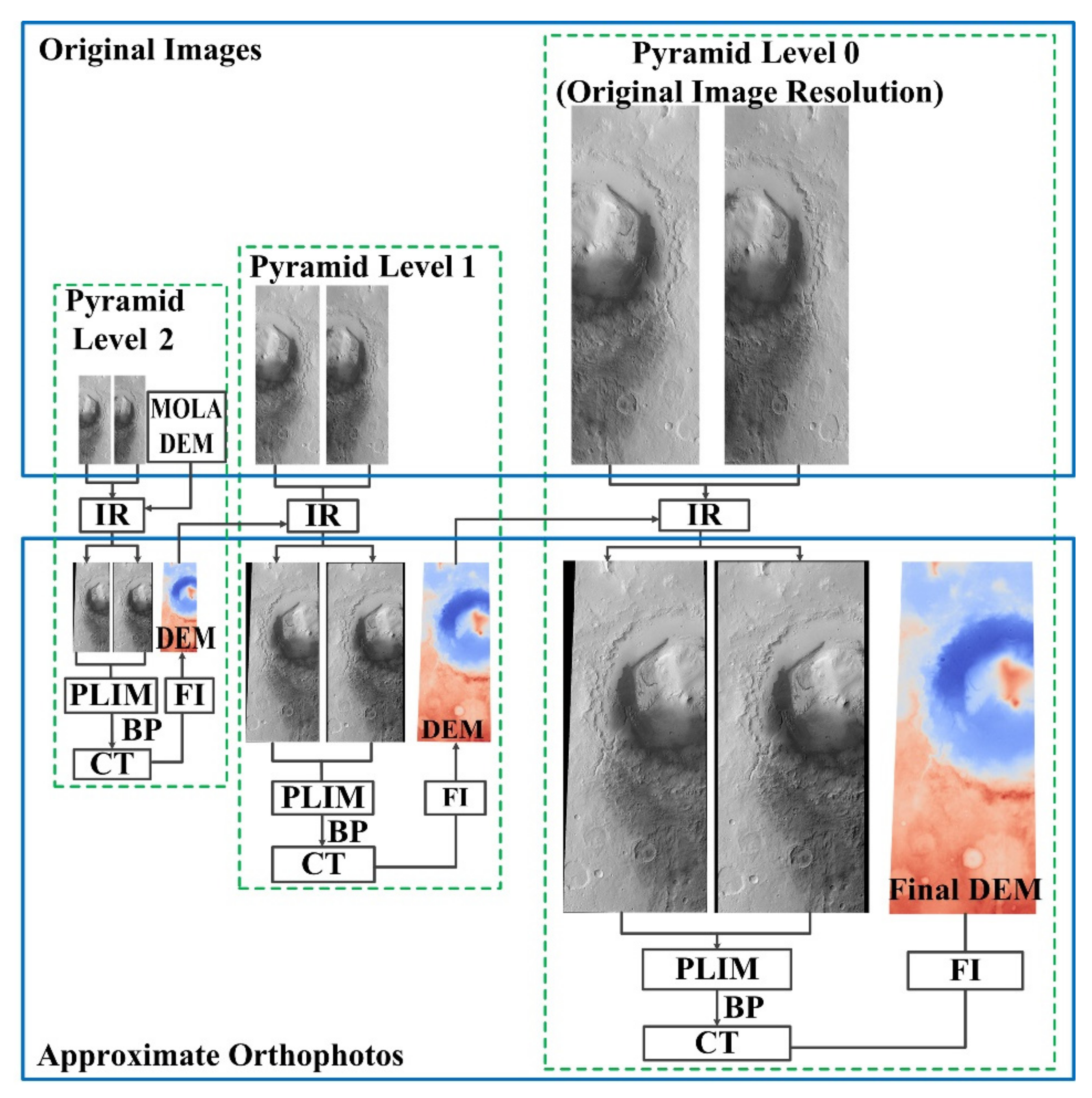
- Suppose that we start from the second pyramid level. Firstly, a rough MOLA DEM is used to perform image rectification, and two approximate orthophotos can be generated using the original HRSC Level-2 S1 and S2 images. Then, the pixel-level image matching is performed on approximate orthophotos instead of original images. The matched points on the approximate orthophotos are converted to the original images. Both image rectification and coordinate transformation of the matched points can use the fast back-projection algorithm described previously.
- (2)
- As shown in Figure 5, the hierarchical image matching strategy is utilized. The matched points at each pyramid level are used to generate DEM through forward intersection.
- (3)
- The generated DEM at the second pyramid level is used as a reference DEM for image rectification at the first pyramid level. Similarly, the generated DEM at the first pyramid level is used as a reference DEM to rectify the original images. Hence, the image distortions caused by perspective projection and terrain relief can be removed by refined DEM. This is very helpful for decreasing the search range.
- (4)
- In the image matching procedure, the approximate positons of conjugate points are estimated using the ground point coordinates of orthophotos, which can efficiently and accurately determine the start point of template matching.
In theory, if the interior orientation (IO) and EO parameters together with the reference DEM are accurate enough, the conjugate points on orthophotos will deliver identical ground point coordinates. As a matter of fact, the IO and EO parameters may have slight errors and the reference DEM available may not be accurate enough at the initial processing stages. These factors will cause the conjugate points on orthophotos to deliver different ground point coordinates. As we have used a hierarchical image matching strategy, the pull-in range of the proposed matching method can be enlarged. Furthermore, the proposed method uses the refined DEM and DOM iteratively, which is also very helpful to improve the estimation accuracy for approximate positions of conjugate points.
2.3.1. Image Matching on Approximate Orthophotos
As we all know, the epipolar geometric constraint is always used in image matching, both for frame images and linear pushbroom images [36,37,38]. However, it is difficult to determine the exact epipolar line equation for linear pushbroom imagery. Moreover, the prerequisite of epipolar resampling for linear cameras [37] may not be suitable for HRSC linear pushbroom imagery, which has variable line exposure duration. The projection trajectory method is always used to establish the epipolar line for linear pushbroom imagery. However, the projection trajectory method requires a good knowledge of height information, which is always not accurately known in advance. Thus, usually a large height range is used, which ensures accuracy but causes a loss in efficiency. Considering the practical problems of epipolar resampling for linear pushbroom imagery, we do not adopt the epipolar geometric constraint in the proposed image matching method. Indeed, due to the fact that the image matching is performed on approximate orthophotos, the geometric constraint introduced by image rectification can be used. The approximate orthophotos can be generated by image rectification using the IO, EO parameters and rough DEM data. Here, “approximate” indicates that the reference DEM used for image rectification is not accurate enough (such as MOLA DEM) or is not the final DEM product.
As illustrated in the top plot of Figure 6, the identical crater marked by the red rectangle shows a different shape between the HRSC Level-2 S1 and S2 channels. Obviously, because of the different viewing angles and image scale, it is difficult to perform image matching on the original HRSC Level-2 images. The HRSC Level-3 images are generated with MOLA DEM, which can be seen as approximate orthophotos. As shown in the bottom plot of Figure 6, the image distortions are removed through image rectification, and the original stereo images are resampled with the identical ground sample distance (GSD). Obviously, it is convenient to perform image matching on the approximate orthophotos. Figure 6 also illustrates a pair of conjugate points on the approximate orthophotos and the original images, respectively. Given an image point on the approximate orthophotos, the corresponding 3D ground point coordinates are calculated with the reference DEM used in the image rectification process. The coordinates transformation from the approximate orthophotos to the original images is indeed a back-projection operation. Thus, the fast back-projection algorithm described in Section 2.2.3 can be utilized.
Here, we point out that when image matching is performed for DEM generation, the IO and EO data are usually accurately known. Thus, given a stereo pair, two orthophotos can be generated through image rectification with the reference DEM. Usually, a rough DEM such as MOLA DEM is available for the initial iteration stage. With hierarchical image matching, the DEM can be refined iteratively. Therefore, if the reference DEM is accurate enough, the coordinate displacements of conjugate points on orthophotos will be very small. This interesting and useful information can be used to estimate the approximate positions of conjugate points. In summary, image matching on approximate orthophotos is especially suitable for the Martian surface, and the main advantages are as follows.
- (1)
- The original stereo images are resampled with the identical ground sample distance (GSD), which is helpful for improving the matching accuracy and success rate.
- (2)
- As previously described, the Martian surface has a continuous topography. Moreover, the image distortions caused by perspective projection and terrain variation are removed by image rectification. Therefore, an area-based image matching method using normalized cross-correlation (NCC) can obtain better matching results for approximate orthophotos.
- (3)
- The coordinates displacements of conjugate points on stereo approximate orthophotos are very small. Therefore, there is no need to perform epipolar resampling, and conjugate points can be determined with a small search range. This indicates that strong geometric constraints for image matching can be introduced implicitly by image rectification.
- (4)
- For the HRSC stereo pairs, due to the fact that the stereo images (such as S1 and S2 channels) are acquired by identical optical cameras, a high relative accuracy can be achieved. Hence the conjugate points on the approximate orthophotos will show small pixel coordinate displacements (PCDs).
2.3.2. Hierarchical Image Matching with Iteratively-Refined DEM
Hierarchical image matching is widely used in many image matching algorithms. Similarly, the proposed method adopts this practical strategy as well. However, further improvement is made for the hierarchical matching strategy. When the pixel-level image matching is completed on approximate orthophotos, the matched points are converted to the original images. Then, the DEM is generated through forward intersection. Moreover, the DEM generated at the current pyramid level is used as reference data for image rectification at the next pyramid level. As previously described, the proposed pixel-level image matching method uses the geometric constraints introduced by image rectification. Therefore, the accuracy of the reference DEM has a great impact on the estimation accuracy for approximate positions for conjugate points. Obviously, through iterative processing, the generated DEM becomes more and more accurate, and the PCDs of conjugate points on approximate orthophotos become smaller and smaller. Consequently, at the highest image resolution level, a small search window such as 5 × 5 is precise enough to determine the conjugate points.
Suppose the original image resolution of HRSC Level-2 images is 25 m and image pyramids are generated with four levels. Hence, the image resolutions for pyramid levels 1–4 are 50 m, 100 m, 200 m, and 400 m, respectively. At the lowest image resolution level, image rectification is carried out using MOLA DEM, which has a grid space of about 500 m. Then, pixel-level image matching at the fourth pyramid level can generate a DEM with a grid spacing of 400 m. This is slightly higher than the grid spacing of MOLA DEMs. The DEM derived at the fourth pyramid level is used as the reference DEM to generate orthophotos at the third pyramid level. Consequently, through hierarchical image matching, the generated DEMs are refined iteratively, and the estimation accuracy for approximate positions of conjugate points will be more accurate.
2.3.3. Estimating Approximate Positions of Conjugate Points
For traditional image matching methods, geometric constraints such as epipolar line or affine transformation are used to estimate the approximate positions of conjugate points [25,26,39]. Using the proposed matching strategies, there is no need to estimate the approximate positions of conjugate points by such a complicated technique. We suggest that the ground point coordinates are used to estimate the approximate positions of conjugate points. Furthermore, the estimation accuracy for approximate positions of conjugate points depends on the accuracy of the reference DEM used in the image rectification process.
Given an image point on the left orthophoto image, the pixel coordinates of point are and the 2D ground point coordinates of point are . Thus, can be calculated.
where are the left bottom corner point coordinates, and and are the image resolution in the and directions, respectively. We suppose that the left and right orthophotos have identical image resolution. Thus, the pixel coordinates of the conjugate point i’ on the right orthophoto can be estimated.
where are the left bottom corner point coordinates.
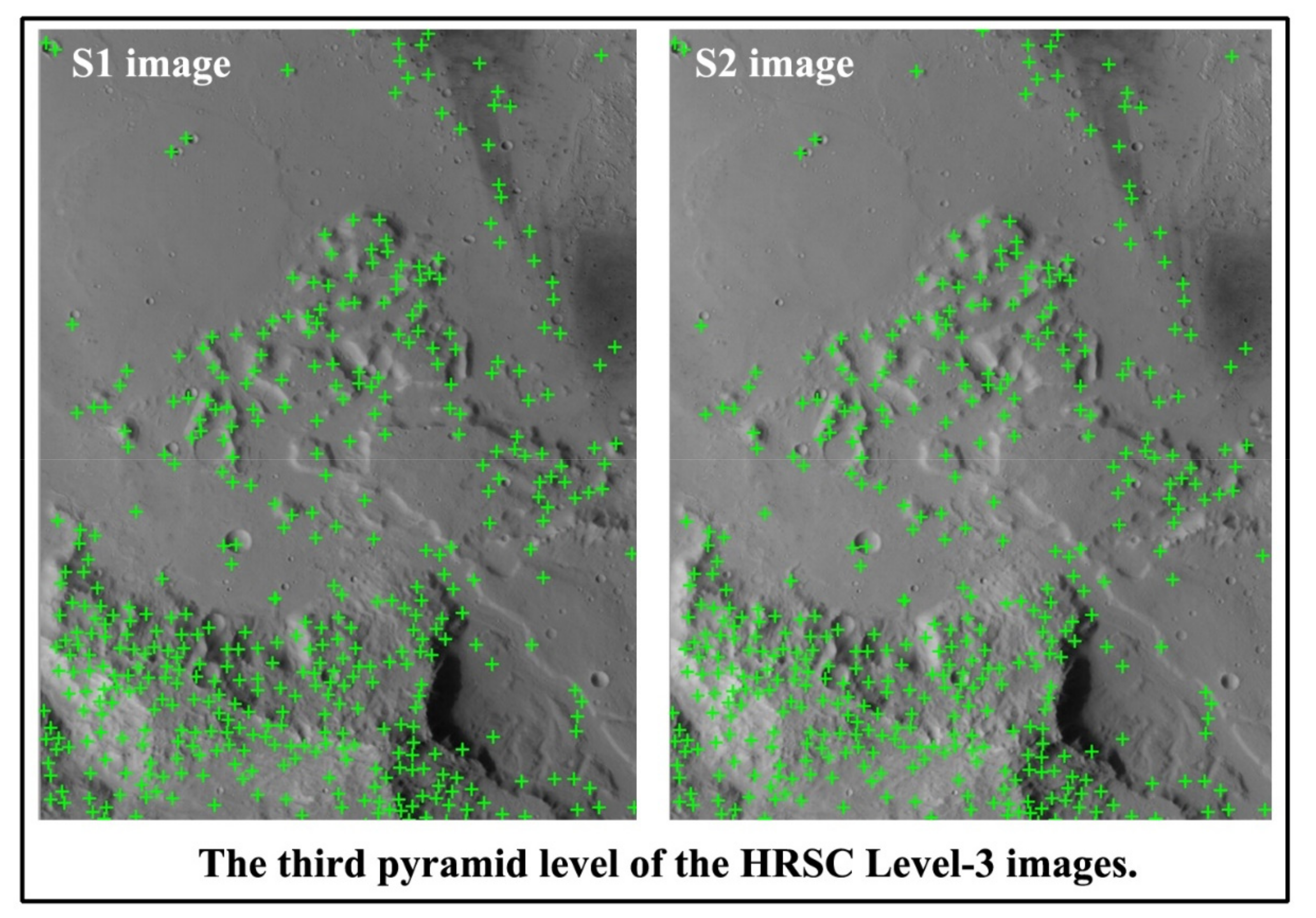
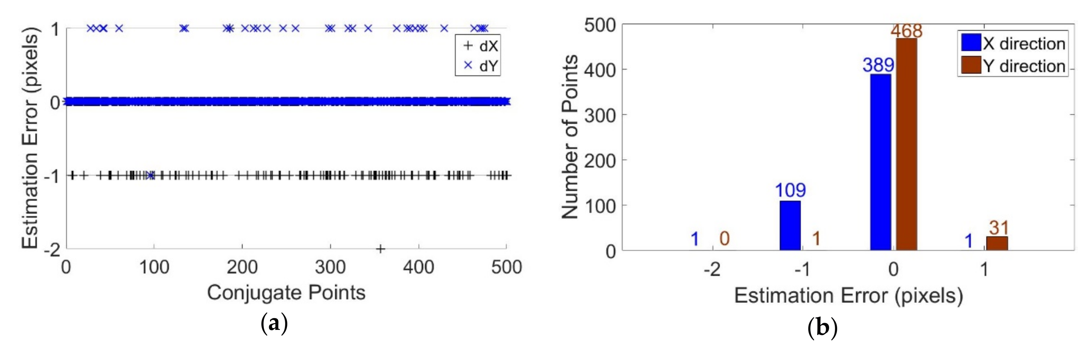
In order to discuss the estimation method for approximate positions of conjugate points, we performed image matching on the third pyramid level of the HRSC Level-3 images. Image matching was carried out between the S1 and S2 channels of orbit 4165. In order to deliver more reliable conjugate points to facilitate the discussion, a high NCC threshold of 0.9 was used. Figure 7 illustrates the matched points on the S1 and S2 channels. Figure 8 shows the PCDs of conjugate points. It is observed that most of the PCDs of conjugate points are less than two pixels in both the and direction. Hence, using the identical pixel coordinates on the left orthophoto as approximate positions, the conjugate point on the right orthophoto can be determined with a 5 × 5 search window. This indicates that at the third pyramid level of approximate orthophotos, the estimation accuracy for approximate positions of conjugate points can reach two pixels. Therefore, conjugate points can be determined efficiently and accurately. Considering that the image resolution of the third pyramid level is eight times lower than the original image resolution, it can be inferred that the maximum PCDs of conjugate points will reach 16 pixels at the original image resolution level. As we noted previously, the HRSC Level-3 images are generated through image rectification using MOLA DEMs. Thus, when the refined DEM is used to generate approximate orthophotos at the higher image resolution level, the PCDs of conjugate points will be decreased further.
2.4. DEM Generation
In theory, multi-view image matching may provide more accurate DEM results. However, in practical scenarios, several factors such as image quality, convergence angle, and image resolution variation have a great influence on the final multi-view image matching results. Moreover, in terms of surface reconstruction, usually a very long period of time is required for dense image matching. Multi-view image matching will multiply the computation time. Liu et al. [40] found that selected stereo photographs with a proper convergence angle can produce better precision than using all the images. Therefore, we use S1 and S2 channels to perform pixel-level image matching to derive DEM. This is because stereo pairs with the largest convergence angle can be formed by the S1 and S2 channels.
2.4.1. DEM Generation Procedure
With the proposed pixel-level image matching method, a higher Mars DEM can be generated using HRSC stereo images. The DEM generation procedure is illustrated in Figure 9.
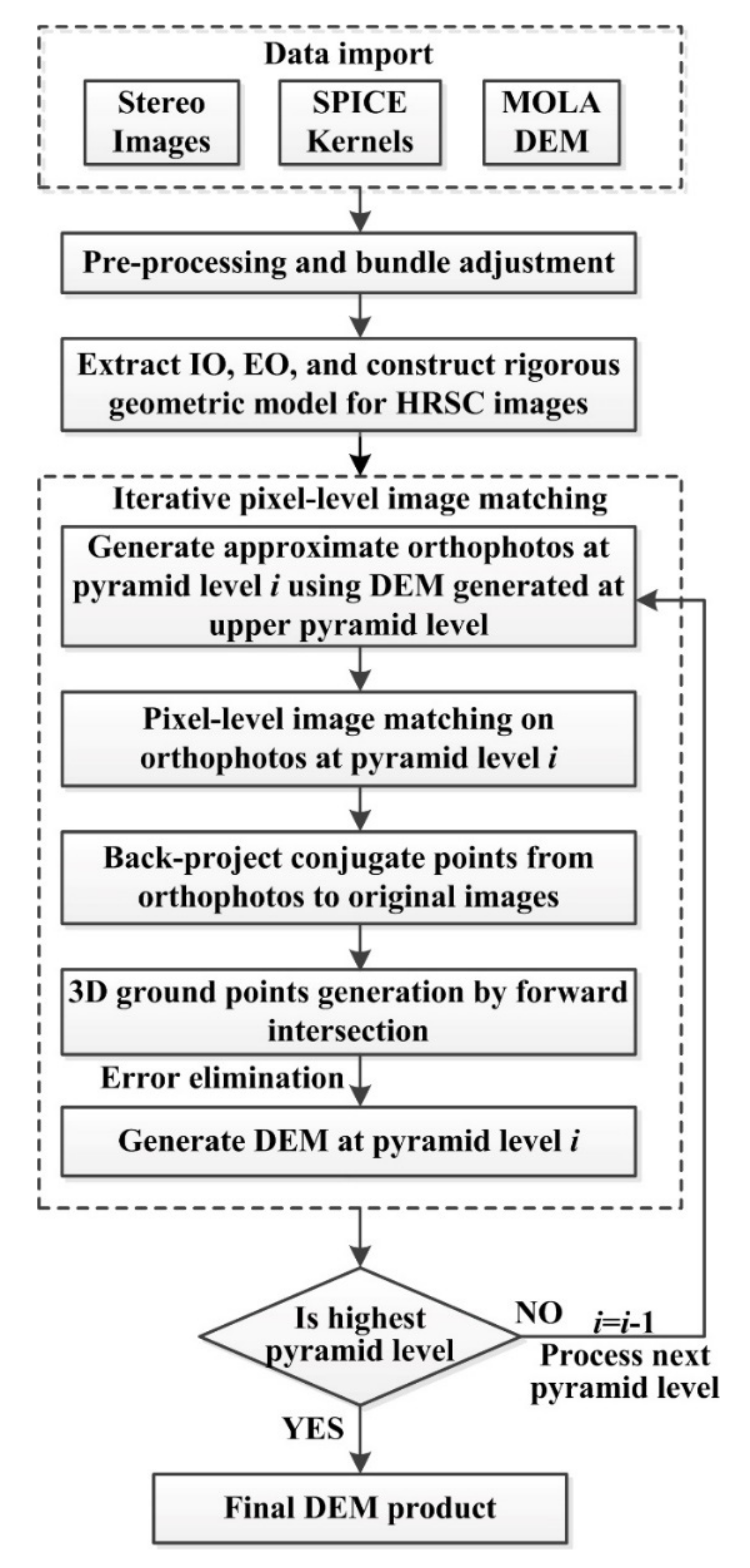
The detailed processing steps for generating DEMs are as follows.
- (1)
- ISIS and SPICE kernels are used to perform data pre-processing. Several programs provided by ISIS are required, including hrsc2isis, spiceinit, tabledump and jigsaw. The HRSC Level-2 images in a raw planetary data system (PDS) format are imported into ISIS using hrsc2isis, and the kernels corresponding to the images are determined with spiceinit.
- (2)
- Data pre-processing including contrast enhancement and image pyramid generation is carried out, which is useful to improve image matching results. The bundle adjustment process is performed with jigsaw.
- (3)
- The IO and EO data are extracted from SPICE kernels. The scan line exposure time parameters are acquired with tabledump. Then, the rigorous geometric model for HRSC linear pushbroom images is constructed using Equation (2).
- (4)
- The DEM is refined iteratively. At the lowest pyramid level, the approximate orthophotos are generated using a rough DEM (MOLA DEM) as reference data. The matched points on orthophotos are converted to the original Level-2 images. Then, the DEMs are generated through forward intersection. The DEM generated at the current pyramid level is used as a source of reference data to generate approximate orthophotos at the next pyramid level.
Through hierarchical image matching, the generated DEM becomes more and more accurate. At last, the grid spacing of the final DEM product at the original image resolution level can reach pixel level. Due to the fact that the DEM used for image rectification is generated iteratively, very accurate approximate positions of conjugate points can be provided at the highest image resolution level. Furthermore, there is no need to extract feature points due to the fact that pixel-level image matching is performed at each pyramid level.
2.4.2. Forward Intersection for HRSC Linear Pushbroom Imagery
The forward intersection for linear pushbroom images is more complicated than frame images. Figure 10 illustrates the processing procedures of forward intersection for HRSC linear pushbroom imagery. and are a pair of conjugate points, () and () are the pixel coordinates for and respectively, () and () are the image point coordinates, () and () are image space coordinates, and () are the 3D ground point coordinates. Firstly, the pixel coordinates on the original images are converted to the image point coordinates using Equation (1). Secondly, the exact EO parameters for scan line and are interpolated using the extracted EO parameters. Then, the image point coordinates are converted to the image space coordinates. Finally, the ground point () is calculated using an extended collinearity equation. It is noteworthy that the ground point coordinates are defined in a body-fixed Martian Cartesian coordinate system. In order to generate a DEM product, map projection and DEM interpolation are required.
2.4.3. Wrongly Matched Points Elimination
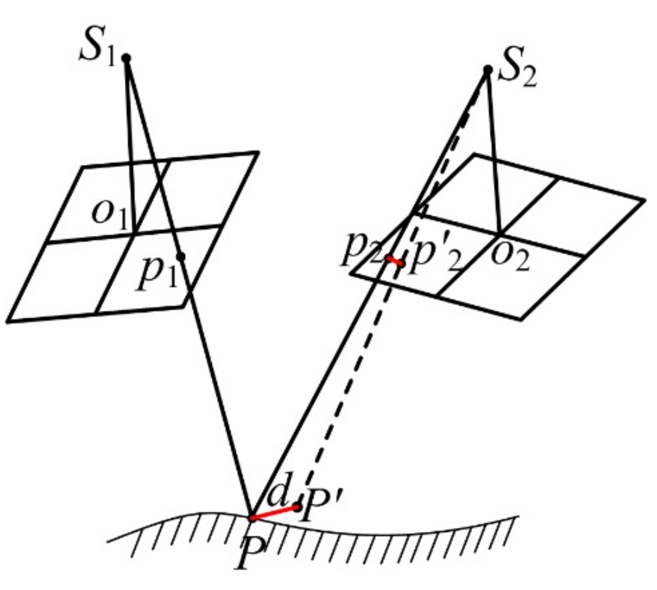
It is impossible for the correct rate of image matching to reach 100 percent. Therefore, it is necessary to eliminate the wrongly matched points. In this paper, the residuals of forward intersection are used to eliminate the wrongly matched points. Suppose there is a pair of conjugate points on stereo images, in the forward intersection procedure there are three unknowns and four observation equations. Thus, the residuals of forward intersection can be computed. Assuming that the IO and EO are accurate enough, the residuals of forward intersection are determined by the image matching accuracy. As shown in Figure 11, image points and are a pair of conjugate points, and is the corresponding ground point. If the image point is wrongly matched as the conjugate point of , a ground point will be determined through forward intersection, and consequently a displacement will be delivered. Therefore, we can give a threshold such as twice of the GSD to eliminate the wrongly matched points.
2.4.4. Comparison with the HRSC Team’s Method
As presented by some researchers [12,18], the DEM generation method used by the HRSC team consists of: (1) quasi-epipolar geometric constraints; (2) area-based multi-image matching; (3) back-projection of matched points to original Level-2 images; and (4) use of SfS to refine the DEM. Here, we compare the proposed DEM generation method with the HRSC team’s method, and a comparison of matching strategies features in Table 4. The comparison results are explained in detail as follows.
- (1)
- Both methods noted the importance of image rectification for image matching in HRSC linear pushbroom imagery. However, epipolar or quasi-epipolar geometric constraints is not used in the proposed method. As previously described, we use geometric constraints introduced by image rectification to restrict the search range.
- (2)
- A multi-image matching method was utilized by the HRSC team, with the merit of generating more accurate DEM results. However, we suggest that S1 and S2 channels be used to generate DEMs because of computation efficiency.
- (3)
- Both methods required that the matched points be converted to the original images. This is referred to as back-projection in the proposed method. However, the detailed back-projection algorithm was not presented in the HRSC team’s method. We realized the significance of the back-projection algorithm for image matching efficiency, and used a fast back-projection method using geometric constraints in object space.
- (4)
- Due to the fact that the proposed method uses a pixel-level image matching strategy, it is not necessary to use the SfS method to refine the generated DEM further.
3. Results
The software development for image matching and image rectification was carried out using Visual Studio 2013 and Qt 5.4.2 on the Windows 7 platform. The rigorous geometric model and forward intersection for HRSC linear pushbroom imagery were implemented based on the open source photogrammetric software DGAP, provided by Dirk Stallmann from Stuttgart University, Stuttgart, Germany [41]. Multithreading programming technology provided by the Qt platform was used to improve the algorithm’s performance, and the tests were performed with four worker threads. The hardware configurations were Intel Core i5 CPU with 8 GB RAM capacity.
3.1. Experimental Datasets
Four test datasets, namely orbits 4165, 5273, 4235 and 5124 were used to verify the proposed method. The test datasets contained different terrain types including craters, mountains and flatland areas. The image width of the HRSC Level-2 S1 and S2 images for orbits 4165 and 5273 is 5184 pixels, which is the default value. In contrast, the S1 and S2 channels of orbits 4235 and 5124 were acquired with the summing mode, and the image width of the Level-2 images is 2584 pixels. Some SPICE kernels are required to perform pre-processing, and include:
- (a)
- spacecraft’s position data: ORMM__070401000000_00387.BSP for orbits 4165 and 4235, ORMM__080201000000_00474.BSP for orbit 5273, and ORMM__071201000000_00457.BSP for orbit 5124;
- (b)
- spacecraft’s orientation data: ATNM_P060401000000_01122.BC;
- (c)
- spacecraft’s clock coefficients: MEX_150108_STEP.TSC;
- (d)
- HRSC’s geometric parameters: MEX_HRSC_V03.TI and hrscAddendum004.ti;
- (e)
- reference frame specifications: MEX_V12.TF;
- (f)
- leapseconds tabulation: naif0010.tls; and
- (g)
- target body (Mars) size, shape and orientation: pck00009.tpc.
These SPICE kernels can be download in the Linux environment using rsync command, and the detailed command line parameters are as follows.
rsync -azv --delete --partial isisdist.astrogeology.usgs.gov::isis3data/mex/kernels
The image pyramids were generated with four pyramid levels using bi-cubic interpolation. The approximate orthophotos were generated with the HRSC Level-2 images using equi-rectangular projection. The Martian reference datum is defined using a sphere body with an axis of 3396.19 km. The search window size is 7 × 7, and the match window size is 9 × 9. In order to match more points with the proposed method, a small NCC threshold is used. The NCC threshold is 0.5 at the original image resolution level and 0.6 at the other pyramid levels. The test datasets information and the image matching time are listed in Table 5.
3.2. Experimental Results
3.2.1. Image Matching Results
Figure 12 presents the image matching cost maps calculated using NCC for the test datasets. We use the S1 channel orthophoto as reference image. For each pixel on the S1 channel orthophoto, a NCC matching is carried out. Then, using the derived NCC matching results, the image matching cost maps can be plotted on the S1 channel orthophotos. As observed in Figure 12a, the regions with low image matching cost are mainly in flatland areas, which show poor image texture. However, the terrain relief information in flatland areas can be interpolated with a small number of conjugate points. Hence, the regions with low image matching cost will not affect the final DEM results. As noted in Figure 12b and the left top part of (d), very high image matching cost (near to 1.0) can be achieved at the rich texture areas such as craters and mountain areas. Consequently, surface reconstruction in these areas will deliver satisfying results.
Since pixel-level image matching is carried out, it is inconvenient to demonstrate all matched points visually. Therefore, for better visual effects we only draw the thinned conjugate points for a small part of the images of orbit 5124. The selected area is marked by a blue rectangle in Figure 12d. The thinned conjugate points are shown with green crosses in Figure 13.
Meanwhile, numbers are used with the green crosses to show the relationship between the matched points on orthophotos and the matched points on the original HRSC Level-2 images. For example, the conjugate points on orthophotos numbered 1 are located in the top left part of the panel, whereas the corresponding conjugate points on the original HRSC Level-2 images are located in the top right part of the panel. Meanwhile, it is observed that the matched points on the approximate orthophotos are precisely converted to the original HRSC Level-2 images. The uniformly distributed matched points on the approximate orthophotos demonstrate the effectiveness of the proposed pixel-level image matching method. Some holes are observed in the shadow region, although this is unavoidable. More image matching results are presented by the generated DEMs in the following section.
3.2.2. Estimation Accuracy for Approximate Positions of Conjugate Points
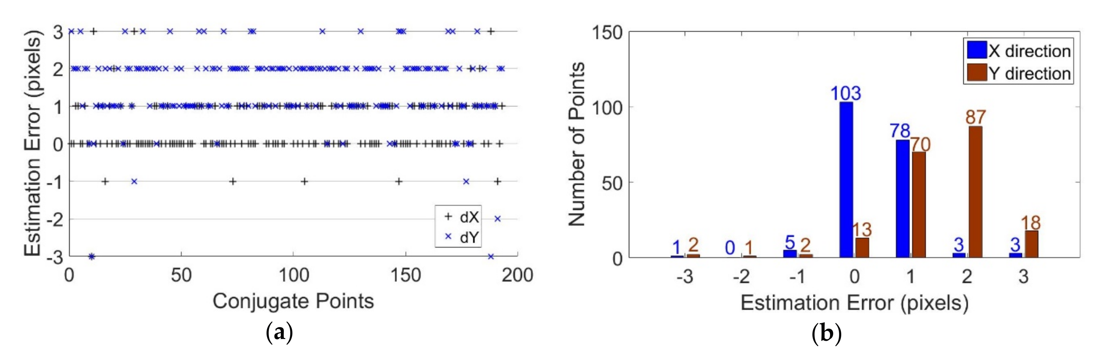
We use the matched points in Figure 13 to discuss the estimation accuracy for approximate positions of conjugate points. Due to that we use the ground point coordinates of the orthophotos to estimate the approximate positions of conjugate points, the PCDs between the matched positions and the estimated approximate positions are utilized to calculate the estimation accuracy. As illustrated in Figure 14, the PCDs for conjugate points on the approximate orthophotos were less than three pixels in both and directions. This indicates that the proposed method can provide very precise approximate positions of conjugate points. The histogram plot, as observed in Figure 14b, illustrates the estimation accuracy in the and directions respectively, which demonstrate that the estimation accuracy in the direction is slightly higher than the estimation accuracy in the direction. Compared with the SIFT matching results as described in Section 2.3.3, the refined DEM improves the estimation accuracy for approximate positions of conjugate points from 16 pixels to three pixels at the original image resolution level. As shown in Figure 15, the conjugate points on the original HRSC Level-2 images have larger PCDs. Moreover, it is observed that the conjugate points on the HRSC Level-2 images show obvious systematic displacements in direction. For one-row conjugate points on the HRSC Level-2 images such as points 1~14, a straight line can be fitted in the direction. Then, if image matching is performed along the fitted straight line, the parallax in the direction can be removed greatly. However, as can be observed, a discrepancy of several pixels still exists. Unfortunately, the PCDs on the HRSC Level-2 images in the direction cannot be fitted with a straight line. This implies that epipolar or quasi-epipolar resampling for HRSC linear pushbroom imagery may not provide effective geometric constraints for image matching. However, as observed in Figure 14, strong geometric constraints for image matching are introduced by image rectification. This clearly illustrates the advantages of image matching on the approximate orthophotos.
3.2.3. DEM Results
The final DEM results are generated through forward intersection using the matched points at the original image resolution level. The grid spacing of the generated DEM is 13 m for orbit 4165 and 25 m for the other orbits, which is almost the same as the image resolution of the original HRSC Level-2 images. Moreover, in order to verify the geometric accuracy of the generated DEM, terrain profiles comparison between the generated DEM and the HRSC Level-4 DEM were carried out. The grid spacing of the sampled points for plotting the terrain profiles is 25 m. We used 800 sampled points to plot the terrain profiles, which are 20 km in length. The positions of the sampled points are marked with a red solid line in the generated DEM.
The generated DEM for orbit 4165 is shown in Figure 16. The extent of the generated DEM is 62 km from east to west and 245 km from north to south. The longitude range of the orbit 4165 is close to 180 degrees east. Therefore, a false easting offset of 10,000 km is used in the longitude direction to decrease the projection coordinates value. The generated DEM is in the elevation of −4000 to −1400 m. As shown in Figure 16b, the sampled points for plotting terrain profile crosses a crater. As illustrated by the terrain profile, the crater’s shape is nicely illustrated. Additionally, the terrain profiles comparison results indicate that the generated DEM coincides with the HRSC Level-4 DEM.
Figure 17a shows the generated DEM results for orbit 5273. A part of the Gale crater is visible on the images, which is where the Mars Curiosity rover landed. As shown in the right part of Figure 17a, the sampled points for plotting terrain profile are near the landing site of the Curiosity rover. Figure 17b also illustrates that there are small systematic errors between the generated DEM and the HRSC Level-4 DEM. The generated DEM is slightly higher than the HRSC Level-4 DEM. This may be caused by the fact that the refined EO parameters used by the proposed method and the HRSC team differs.
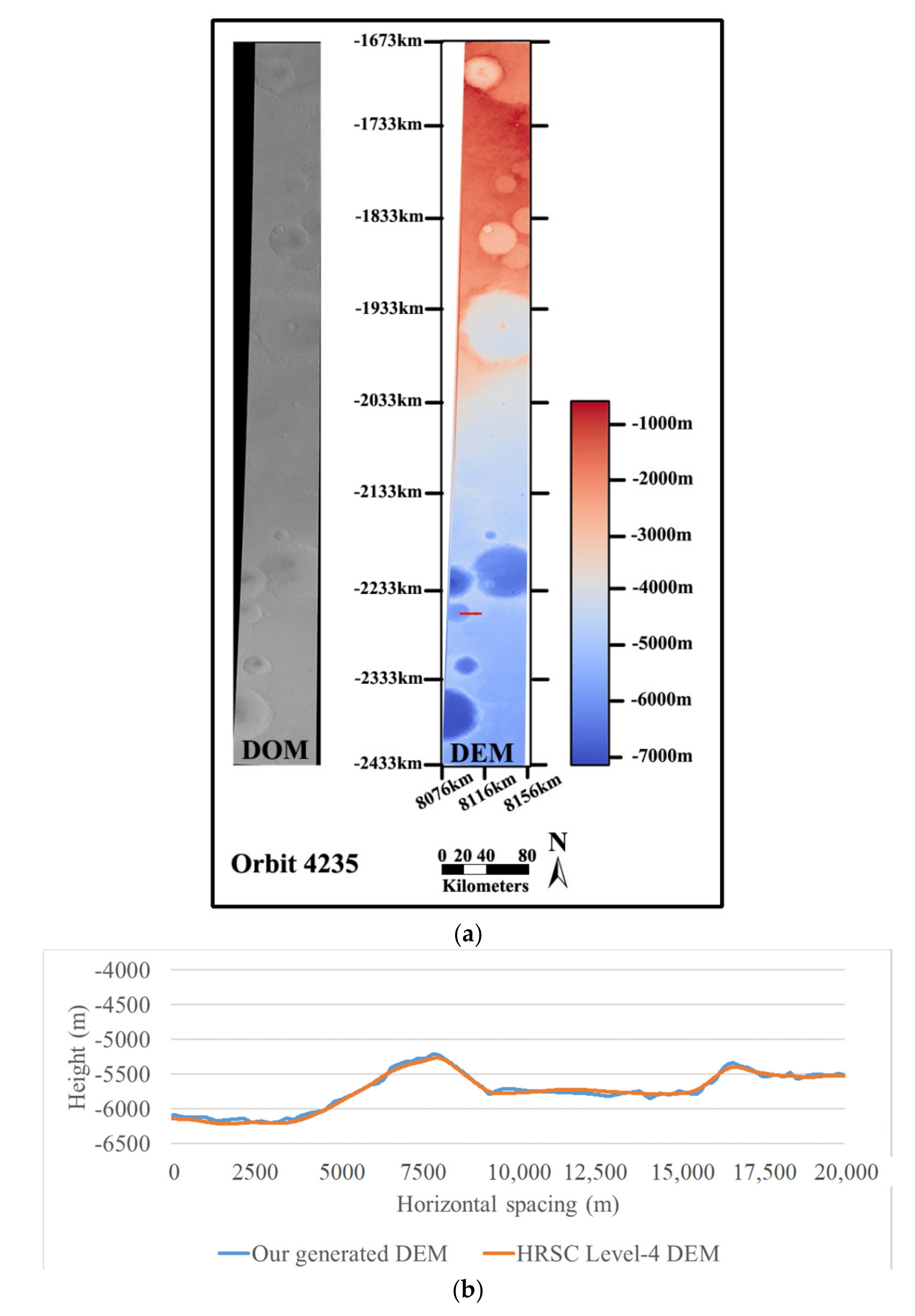
As illustrated in Figure 18a, many craters are observed on orbit 4235 images. The diameters of these craters vary from several kilometers to 60 km. It is noted that the terrain relief of these craters was well reconstructed. The generated DEM is in the elevation of −7100 to −700 m. The 4235 orbit images have more than 30,000 scan lines. Hence, the generated DEM is about 760 km in latitude. As observed in Figure 18b, the generated DEM fits the HRSC Level-4 DEM.
Figure 19 shows the generated DEM results for orbit 5124 images. The top half of the orbit 5124 images shows rich texture information. As shown in Figure 19a, the generated DEM express the complicated terrain relief very well. In Figure 19b, slight biases between the generated DEM and HRSC Level-4 DEM are observed.
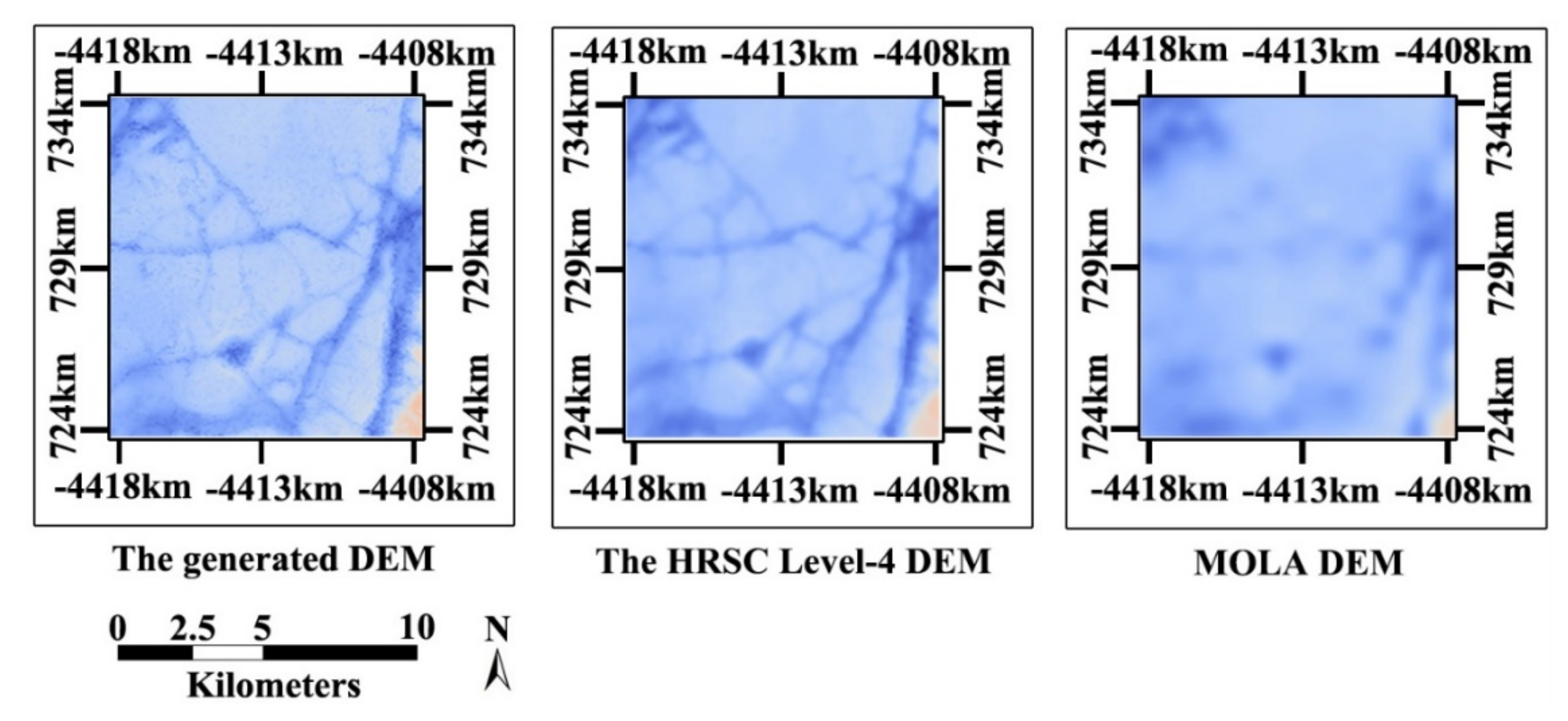
In order to further present the pixel-level image matching results, visual comparison among the generated DEM, HRSC Level-4 DEM, and MOLA DEM was performed. The HRSC Level-4 DEM and MOLA DEM are resampled with a grid spacing of 25 m, which is the same as the grid spacing of the generated DEM. The comparison region is marked with a blue rectangle in Figure 19a. The results are presented in Figure 20. As can be observed, the generated DEM shows more terrain relief details. Meanwhile, the generated DEM also shows some noise, which is mainly caused by some inaccurate conjugate points.
3.2.4. DEM Accuracy Analysis
In order to better discuss the accuracy of the generated DEM, the height displacements between the generated DEM and HRSC Level-4 DEM are calculated using uniformly distributed sampled points in the whole domain of the DEM. Because the resolution of the generated DEM is superior to the HRSC Level-4 DEM, image resampling is required. Firstly, the HRSC Level-4 DEMs are resampled with the grid spacing of the generated DEM as described in Section 3.2.3. The sampling intervals for calculating height displacements are 20 GSD in both row and column directions. Then, the height displacements are calculated by subtracting the two values computed at the same sampled points. Consequently, the maximum value, mean value and root mean square errors (RMSE) of height displacements are calculated, and the results are presented in Table 6.
As observed in Table 6, the maximum value of height displacements for the test datasets are 81.6 m (6.3 pixels), 76.3 m (3.1 pixels), 93.8 m (3.8 pixels) and 79.2 m (3.2 pixels), respectively. A high maximum value of height displacements may be caused by the wrongly matched points. As observed, orbit 4235 delivers the highest maximum value of height displacements, and results in 93.8 m. The mean value of height displacements can be used to analyze the systematic errors. As observed, the mean values of height displacements for the four test datasets are 25.4 m (2.0 pixels), 30.5 m (1.2 pixels), 25.1 m (1.0 pixels) and 40.9 m (1.6 pixels) respectively. This indicates that there is about 1~2 pixels of systematic error between the generated DEM and the HRSC Level-2 DEM. The RMSE values of height displacements are 31.3 m (2.4 pixels), 34.5 m (1.4 pixels), 30.2 m (1.2 pixels) and 28.6 m (1.1 pixels) respectively. The small RMSE values indicate that the generated DEM fits the HRSC Level-4 DEM. In summary, as observed in the terrain profiles and Table 6, though slight systematic errors are observed, the generated DEM show good consistency with the HRSC Level-4 DEM.
4. Discussion
Many factors may influence the image matching results, including terrain types, matching strategies, search window size, NCC threshold etc. As illustrated by the image matching cost maps shown in Figure 12, the terrain types of the test datasets have a great impact on the NCC matching cost values. Flatland areas in orbit 4165 and 4235 delivered small NCC matching cost values, which are usually less than 0.5. In contrast, as observed in orbit 5124 and 5273, craters and mountain areas generally deliver a high NCC matching cost values, which are higher than 0.9. Indeed, image matching may fail in the flatland areas. However, this will not affect the surface reconstruction results after DEM interpolation, which was illustrated by the generated DEM.
As illustrated in Figure 8 and Figure 14, the approximate positions of conjugate points can be estimated with an accuracy of two pixels at the third pyramid level and three pixels at the original image resolution level. Hence, hierarchical image matching with iteratively-refined DEM provides good estimation accuracy for approximate positions of conjugate points. Thus, at each pyramid level, we can use a very small search window such as to determine the conjugate points. Additionally, Figure 14 and Figure 15 demonstrate the advantages of image matching on approximate orthophotos. In contrast, if image matching is performed on the original images, a large search window such as must be used to correctly determine the conjugate points. This will greatly increase the image matching computation cost and introduce wrongly matched points. Furthermore, the computation efficiency of area-based image matching has a linear correlation with image size (height and width ), search window () and template window () size. Specifically, the algorithm complexity of the proposed pixel-level image matching method can be described as , where . Take orbit 5273 as an example, as shown in Table 5, the image height and width of the S1 channel of the HRSC Level-2 image for orbit 5273 are 18,544 and 5176 respectively, and pixel-level image matching was accomplished within 1.96 h. This indicates that about 13,600 conjugate points can be determined per second. In contrast, suppose that the image matching was carried out on the original images, and the search window size is enlarged from to . Then, as can be predicted, the computation time for pixel-level image matching will increase by about nine times. In summary, the proposed algorithm has the advantage of reducing the search window size and improving the computation efficiency.
With the proposed method, a higher resolution Mars DEM is generated. It is observed that the generated DEM shows more terrain variation, which was derived by the pixel-level image matching strategy adopted in the proposed method. All four test datasets show that the generated DEM shows good consistency with the HRSC Level-4 DEM. However, as illustrated by the terrain profiles comparison results and the DEM accuracy analysis results, the generated DEM shows slight systematic errors compared with the HRSC Level-4 DEM, because the EO parameters acquired from SPICE kernels are different from the final EO parameters used by the HRSC team. As described by the output results obtained from spiceinit, the position data of HRSC images obtained from SPICE kernels is reconstructed, whereas the pointing data are only predicted values.
5. Conclusions
In this paper, a novel pixel-level image matching method for MEX HRSC linear pushbroom imagery is proposed. We strongly suggest that the image matching is performed on approximate orthophotos to generate a dense DEM. Based on the experimental results, the following conclusions can be drawn.
- (1)
- We use the derived DEM at current pyramid level to generate orthophotos at the next pyramid level. Hence the proposed image matching method has the advantage that the a priori knowledge at each pyramid level is used to the greatest extent possible. This characteristic strategy greatly improves the image matching efficiency and accuracy.
- (2)
- Though the epipolar resampling method is not utilized by the proposed image matching method, strong geometric constraints can be introduced through image rectification. Hence, it is verified that the use of pixel coordinates of orthophotos to estimate the approximate positions of conjugate points is a practical method.
- (3)
- The pixel-level image matching method generally results in very long processing times. For a typical stereo pair of HRSC images with about 20,000 scan lines, pixel-level image matching can be accomplished within three hours using a normal personal computer. Hence, the computation efficiency of the proposed method is satisfied for pixel-level image matching.
- (4)
- We also noted that the generated DEM exhibits some deficiencies. In low contrast areas, area-based image matching may fail, and results in pointless regions. Additionally, some noise caused by inaccurate matched points should be processed by a small amount of manual editing.
Furthermore, though the proposed method is primarily designed for the MEX HRSC, the basic principle can be used to process other Mars imaging instruments such as MOC and HiRISE. In this paper, we pay great attention to the computation efficiency, considering that pixel-level image matching usually has a very long processing time. Through algorithm optimization such as fast back-projection, using geometric constraints introduced by image rectification and multithreading programming, a pixel-level DEM can be generated with an acceptable time cost. In order to make the proposed method more practical, it shall be optimized with GPU parallel processing in the future.
Acknowledgments
This research was supported by the National Natural Science Foundation of China with project numbers 41401533 and 41371436, and the National Basic Research Program of China with project number 2012CB720000. We would like to thank Professor Wang Mi (Wuhan University, Wuhan, China) for proposing the exact scan line searching method for the airborne linear pushbroom images, which was adopted and modified in our research to process the Mars Express HRSC images. We thank the HRSC team for providing the HRSC products to the public. We also thank Professor Dirk Stallmann (Stuttgart University, Stuttgart, Germany) for providing the open source photogrammetric software DGAP to the public. We would also thank the anonymous reviewers for the constructive suggestions and comments.
Author Contributions
Xun Geng designed the study and wrote the paper. Qing Xu designed the experiments. Shuai Xing and Chaozhen Lan contributed to the discussions and editing. Junyi Xu performed the experiments.
Conflicts of Interest
The authors declare no conflict of interest.
References
- Wu, S.S.C.; Elassal, A.A.; Jordan, R.; Schafer, F.J. Photogrammetric application of Viking orbital photography. Planet. Space Sci. 1982, 30, 45–53. [Google Scholar] [CrossRef]
- Kirk, R.L.; Kraus, E.H.; Rosiek, M. Recent planetary topographic mapping at the USGS, Flagstaff: Moon, Mars, Venus, and beyond. In Proceedings of the International Archives of Photogrammetry, Remote Sensing and Spatial Information Sciences, Amsterdam, The Netherlands, 16–22 July 2000; pp. 476–490. [Google Scholar]
- Kirk, R.L.; Kraus, E.H.; Redding, B.; Galuszka, D.; Hare, T.M.; Archinal, B.A.; Soderblom, L.A.; Barrett, J.M. High-resolution topomapping of candidate MER landing sites with Mars Orbiter Camera narrow-angle images. J. Geophys. Res. Planets 2003, 108, 8088. [Google Scholar] [CrossRef]
- Kirk, R.L.; Kraus, E.H.; Rosiek, R.M.; Anderson, J.A.; Archinal, B.A.; Becker, K.J.; Cook, D.A.; Galuszka, D.M.; Geissler, P.E.; Hare, T.M.; et al. Ultrahigh resolution topographic mapping of Mars with MRO HiRISE stereo images: Meter-scale slopes of candidate Phoenix landing sites. J. Geophys. Res. Planets 2008, 113, 5578–5579. [Google Scholar] [CrossRef]
- Di, K.C.; Xu, F.; Wang, J.; Agarwal, S.; Brodyagina, E.; Li, R.X.; Matthies, L. Photogrammetric processing of rover imagery of the 2003 Mars Exploration Rover mission. ISPRS J. Photogramm. Remote Sens. 2008, 63, 181–201. [Google Scholar] [CrossRef]
- Wu, S.S.C. Extraterrestrial photogrammetry. In Manual of Photogrammetry, 6th ed.; McGlone, J.C., Ed.; American Society for Photogrammetry and Remote Sensing: Bethesda, MD, USA, 2013; pp. 1139–1152. [Google Scholar]
- Jones, E.; Caprarelli, G.; Mills, F.P.; Doran, B.; Clarke, J. An alternative approach to mapping thermophysical units from Martian thermal inertia and albedo data using a combination of unsupervised classification techniques. Remote Sens. 2014, 6, 5184–5237. [Google Scholar] [CrossRef]
- Price, M.A.; Ramsey, M.S.; Crown, D.A. Satellite-based thermophysical analysis of volcaniclastic deposits: A terrestrial analog for mantled lava flows on Mars. Remote Sens. 2016, 8, 152. [Google Scholar] [CrossRef]
- Edmundson, K.L.; Cook, D.A.; Thomas, O.H.; Archinal, B.A.; Kirk, R.L. Jigsaw: The ISIS3 bundle adjustment for extraterrestrial photogrammetry. In Proceedings of the International Archives of Photogrammetry, Remote Sensing and Spatial Information Sciences, Melbourne, Australia, 25 August–1 September 2012; pp. 203–208. [Google Scholar]
- Shean, D.E.; Alexandrov, O.; Moratto, Z.M.; Smith, B.E.; Joughin, I.R.; Porter, C.; Morin, P. An automated, open-source pipeline for mass production of digital elevation models (DEMs) from very-high-resolution commercial stereo satellite imagery. ISPRS J. Photogramm. Remote Sens. 2016, 116, 101–117. [Google Scholar] [CrossRef]
- Albertz, J.; Attwenger, M.; Barrett, J.; Casley, S.; Dorninger, P.; Dorrer, E.; Ebner, H.; Gehrke, S.; Giese, B.; Gwinner, K.; et al. HRSC on Mars Express—Photogrammetric and cartographic research. Photogramm. Eng. Remote Sens. 2005, 71, 1153–1166. [Google Scholar] [CrossRef]
- Scholten, F.; Gwinner, K.; Roatsch, T.; Matz, K.D.; Wahlisch, M.; Giese, B.; Oberst, J.; Jaumann, R.; Neukum, G. The HRSC Co-Investigator Team. Mars Express HRSC data processing—Methods and operational aspects. Photogramm. Eng. Remote Sens. 2005, 71, 1143–1152. [Google Scholar] [CrossRef]
- Rosiek, M.R.; Kirk, R.L.; Archinal, B. Utility of Viking Orbiter images and products for Mars mapping. Photogramm. Eng. Remote Sens. 2005, 71, 1187–1195. [Google Scholar] [CrossRef]
- Shan, J.; Yoon, J.; Lee, D.S.; Kirk, R.L.; Neumann, G.A.; Acton, C.H. Photogrammetric analysis of the Mars Global Surveyor mapping data. Photogramm. Eng. Remote Sens. 2005, 71, 97–108. [Google Scholar] [CrossRef]
- Li, R.X.; Hwangbo, J.; Chen, Y.H.; Di, K.C. Rigorous photogrammetric processing of HiRISE stereo imagery for Mars topographic mapping. IEEE Trans. Geosci. Remote Sens. 2011, 49, 2558–2572. [Google Scholar]
- Hirschmüller, H.; Mayer, H.; Neukum, G. Stereo processing of HRSC Mars Express images by Semi-Global Matching. In Proceedings of the International Archives of Photogrammetry, Remote Sensing and Spatial Information Sciences, Goa, India, 25–30 September 2006. [Google Scholar]
- Heipke, C.; Oberst, J.; Albertz, J.; Attwenger, M.; Dorninger, P.; Dorrer, E.; Ewe, M.; Gehrke, S.; Gwinner, K.; Hirschmuller, H. Evaluating planetary digital terrain models—The HRSC DTM test. Planet. Space Sci. 2007, 55, 2173–2191. [Google Scholar] [CrossRef]
- Gwinner, K.; Scholten, F.; Spiegel, M.; Schmidt, R.; Giese, B.; Oberst, J.; Heipke, C.; Jaumann, R.; Neukum, G. Derivation and validation of high-resolution digital terrain models from mars express HRSC data. Photogramm. Eng. Remote Sens. 2009, 75, 1127–1142. [Google Scholar] [CrossRef]
- Sidiropoulos, P.; Muller, J. Batch co-registration of Mars high-resolution images to HRSC MC11-E mosaic. In Proceedings of the International Archives of Photogrammetry, Remote Sensing and Spatial Information Sciences, Prague, Czech Republic, 12–19 July 2016; Volume XLI, Part B4, pp. 491–495. [Google Scholar]
- Geng, X.; Xu, Q.; Lan, C.Z.; Xing, S. An iterative pixel-level image matching method for Mars mapping using approximate orthophotos. In Proceedings of the International Archives of Photogrammetry, Remote Sensing and Spatial Information Sciences, Hong Kong, China, 13–16 August 2017; pp. 41–48. [Google Scholar]
- Gruen, A. Development and status of image matching in photogrammetry. Photogramm. Rec. 2012, 27, 36–57. [Google Scholar] [CrossRef]
- Haala, N. The landscape of dense image matching algorithms. In Proceedings of the Photogrammetric Week ’13, Stuttgart, Germany, 9–13 September 2013; pp. 271–284. [Google Scholar]
- Zhang, Y.F.; Zhang, Y.J.; Mo, D.L.; Zhang, Y.; Li, X. Direct digital surface model generation by semi-global vertical line locus matching. Remote Sens. 2017, 9, 214. [Google Scholar] [CrossRef]
- Shao, Z.; Yang, N.; Xiao, X.; Zhang, L.; Peng, Z. A multi-view dense point cloud generation algorithm based on low-altitude remote sensing images. Remote Sens. 2016, 8, 381–397. [Google Scholar] [CrossRef]
- Zhang, L.; Gruen, A. Multi-image matching for DSM generation from IKONOS imagery. ISPRS J. Photogramm. Remote Sens. 2006, 60, 195–211. [Google Scholar] [CrossRef]
- Hirschmüller, H. Stereo processing by Semi-Global Matching and mutual information. IEEE Trans. Pattern Anal. Mach. Intell. 2008, 30, 328–341. [Google Scholar] [CrossRef] [PubMed]
- Furukawa, Y.; Ponce, J. Accurate, dense, and robust multiview stereopsis. IEEE Trans. Pattern Anal. Mach. Intell. 2010, 32, 1362–1376. [Google Scholar] [CrossRef] [PubMed]
- Wenzel, K.; Rothermel, M.; Haala, N.; Fritsch, D. SURE—The ifp software for dense image matching. In Proceedings of the Photogrammetric Week ’13, Stuttgart, Germany, 9–13 September 2013; pp. 59–70. [Google Scholar]
- Wu, B.; Liu, W.C.; Grumpe, A.; Wohler, C. Shape and albedo from shading (SAfS) for pixel-level DEM generation from monocular images constrained by low-resolution DEM. In Proceedings of the International Archives of Photogrammetry, Remote Sensing and Spatial Information Sciences, Prague, Czech Republic, 12–19 July 2016; Volume XLI, pp. 521–527. [Google Scholar]
- Acton, C.; Bachman, N.; Semenov, B.; Wright, E. SPICE tools supporting planetary remote sensing. In Proceedings of the International Archives of Photogrammetry, Remote Sensing and Spatial Information Sciences, Prague, Czech Republic, 12–19 July 2016; pp. 357–359. [Google Scholar]
- Ogohara, K.; Kouyama, T.; Yamamoto, H.; Sato, N.; Takagi, M.; Imamura, T. Automated cloud tracking system for the Akatsuki Venus Climate Orbiter data. Icarus 2012, 217, 661–668. [Google Scholar] [CrossRef]
- Kim, T.; Lee, Y.; Shin, D. Development of a robust algorithm for transformation of a 3D object point onto a 2D image point for linear pushbroom imagery. Photogramm. Eng. Remote Sens. 2001, 67, 449–452. [Google Scholar]
- Wang, M.; Hu, F.; Li, J.; Pan, J. A fast approach to best scanline search of airborne linear pushbroom images. Photogramm. Eng. Remote Sens. 2009, 75, 1059–1067. [Google Scholar] [CrossRef]
- Zhao, S.M.; Li, D.R.; Mou, L.L. Inconsistency analysis of CE-1 stereo camera images and laser altimeter data. Acta Geod. Cartogr. Sin. 2011, 40, 751–755. [Google Scholar]
- Geng, X.; Xu, Q.; Xing, S.; Lan, C.Z.; Hou, Y.F. Differential rectification of linear pushbroom imagery based on the fast algorithm for best scan line searching. Acta Geod. Cartogr. Sin. 2013, 42, 861–868. [Google Scholar]
- Kim, T. A study on the epipolarity of linear pushbroom images. Photogramm. Eng. Remote Sens. 2000, 66, 961–966. [Google Scholar]
- Morgan, M.; Kim, K.; Jeong, S.; Habib, A. Epipolar resampling of space-borne linear array scanner scenes using parallel projection. Photogramm. Eng. Remote Sens. 2006, 72, 1255–1263. [Google Scholar] [CrossRef]
- Wang, M.; Hu, F.; Li, J. Epipolar resampling of linear pushbroom satellite imagery by a new epipolarity model. ISPRS J. Photogramm. Remote Sens. 2011, 66, 347–355. [Google Scholar] [CrossRef]
- Afsharnia, H.; Arefi, H.; Sharifi, M.A. Optimal weight design approach for the geometrically-constrained matching of satellite stereo images. Remote Sens. 2017, 9, 965. [Google Scholar] [CrossRef]
- Liu, B.; Jia, M.N.; Di, K.C.; Oberst, J.; Xu, B.; Wan, W.H. Geopositioning precision analysis of multiple image triangulation using LROC NAC lunar images. Planet. Space Sci. 2017, in press. [Google Scholar] [CrossRef]
- DGAP Software. Available online: http://www.ifp.uni-stuttgart.de/publications/software/openbundle/index.en.html (accessed on 10 November 2017).
Figure 1.
The illustration of the terrain characteristics of the Martian surface using the HRSC Level-2 images of orbit 5273. The default pixel data type of the High Resolution Stereo Camera (HRSC) Level-2 images is 16-bit integer, whereas the histograms only plot the valid values between 0 and 255.

Figure 2.
Focal plane arrangement of the High Resolution Stereo Camera (HRSC). S1, S2, P1, P2 and ND represent five panchromatic channels; IR represents near-infrared channel; RE, GR and BL represent red, green and blue channels respectively.
Figure 2.
Focal plane arrangement of the High Resolution Stereo Camera (HRSC). S1, S2, P1, P2 and ND represent five panchromatic channels; IR represents near-infrared channel; RE, GR and BL represent red, green and blue channels respectively.

Figure 3.
Converting the default frame definition acquired from Spacecraft, Planet, Instrument, C-Matrix, Events (SPICE) kernels to the traditional photogrammetric frame definition.
Figure 3.
Converting the default frame definition acquired from Spacecraft, Planet, Instrument, C-Matrix, Events (SPICE) kernels to the traditional photogrammetric frame definition.

Figure 4.
The illustration of exact scan line determination using the geometric constraints in object space.
Figure 4.
The illustration of exact scan line determination using the geometric constraints in object space.

Figure 5.
The basic principle of the proposed pixel-level image matching method. MOLA: Mars Orbiter Laser Altimeter; DEM: digital elevation model; IR: image rectification; PLIM: pixel-level image matching; BP: back-projection; CT: coordinate transformation; FI: forward intersection.
Figure 5.
The basic principle of the proposed pixel-level image matching method. MOLA: Mars Orbiter Laser Altimeter; DEM: digital elevation model; IR: image rectification; PLIM: pixel-level image matching; BP: back-projection; CT: coordinate transformation; FI: forward intersection.

Figure 6.
Stereo pair comparison between the HRSC Level-2 and Level-3 images.
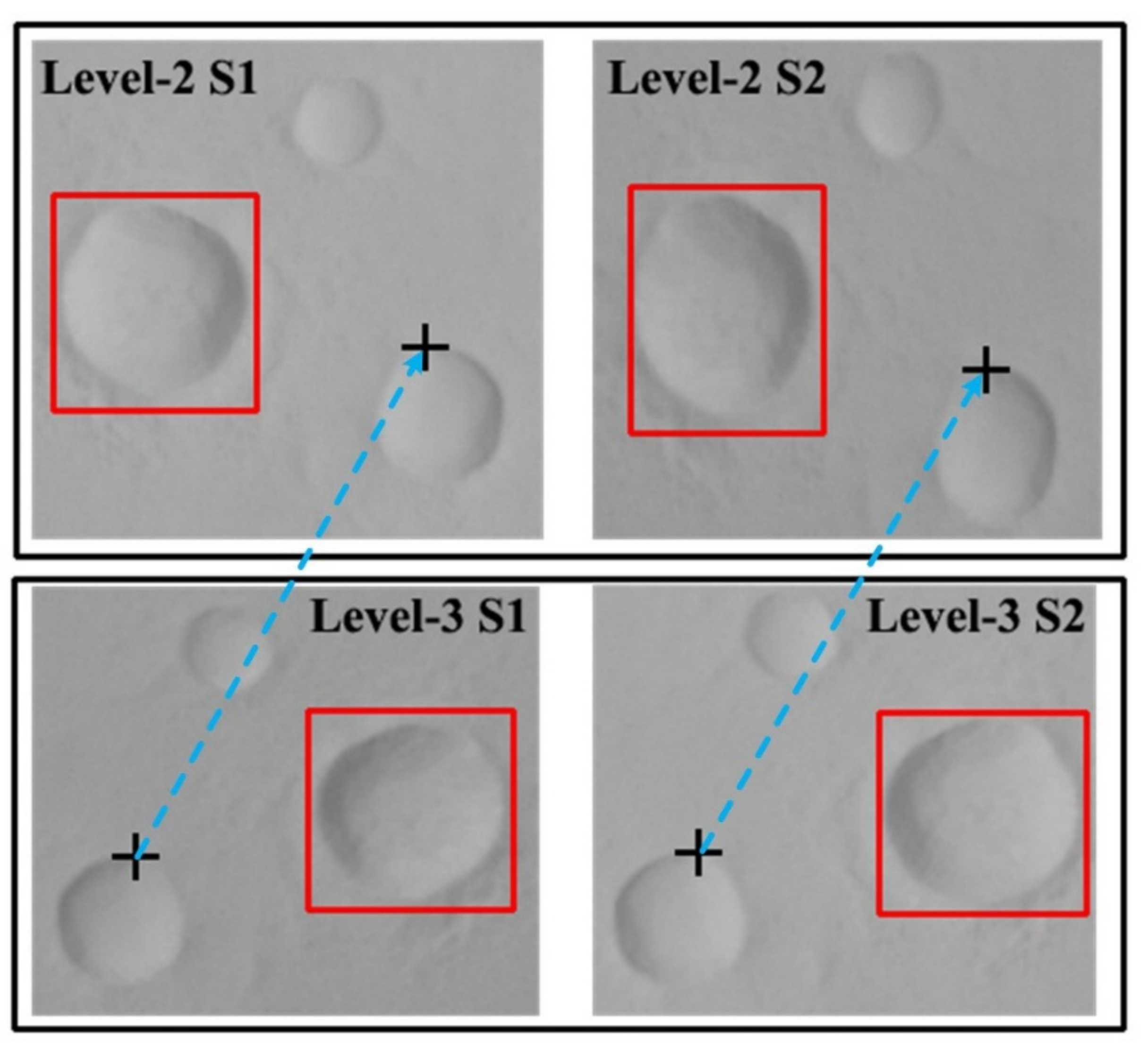
Figure 7.
Image matching results at the third pyramid level of the HRSC Level-3 images.

Figure 8.
Estimation accuracy for approximate positions of conjugate points at the third pyramid level of the HRSC Level-3 images for orbit 4165: (a) scatter chart; and (b) histogram chart.
Figure 8.
Estimation accuracy for approximate positions of conjugate points at the third pyramid level of the HRSC Level-3 images for orbit 4165: (a) scatter chart; and (b) histogram chart.

Figure 9.
The digital elevation model (DEM) generation procedure using the proposed pixel-level image matching method. IO: interior orientation; EO: exterior orientation; SPICE: Spacecraft, Planet, Instrument, C-Matrix, Events.
Figure 9.
The digital elevation model (DEM) generation procedure using the proposed pixel-level image matching method. IO: interior orientation; EO: exterior orientation; SPICE: Spacecraft, Planet, Instrument, C-Matrix, Events.

Figure 10.
The processing procedure of forward intersection for HRSC linear pushbroom imagery.
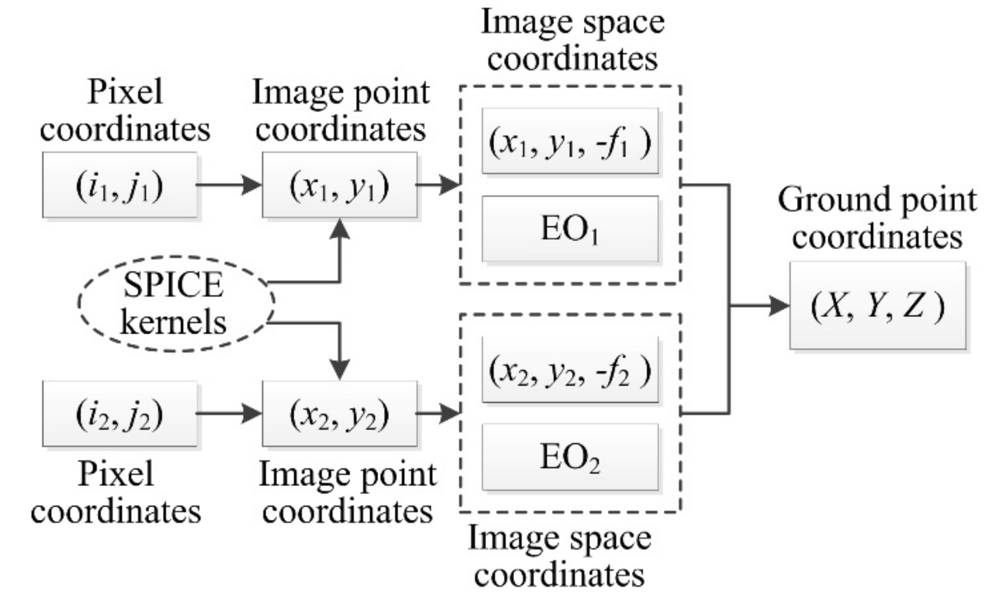
Figure 11.
The illustration of using forward intersection residuals to eliminate wrongly matched points.
Figure 11.
The illustration of using forward intersection residuals to eliminate wrongly matched points.

Figure 12.
Image matching cost maps calculated using normalized cross-correlation (NCC): (a) Orbit 4165; (b) Orbit 5273; (c) Orbit 4235; and (d) Orbit 5124.
Figure 12.
Image matching cost maps calculated using normalized cross-correlation (NCC): (a) Orbit 4165; (b) Orbit 5273; (c) Orbit 4235; and (d) Orbit 5124.
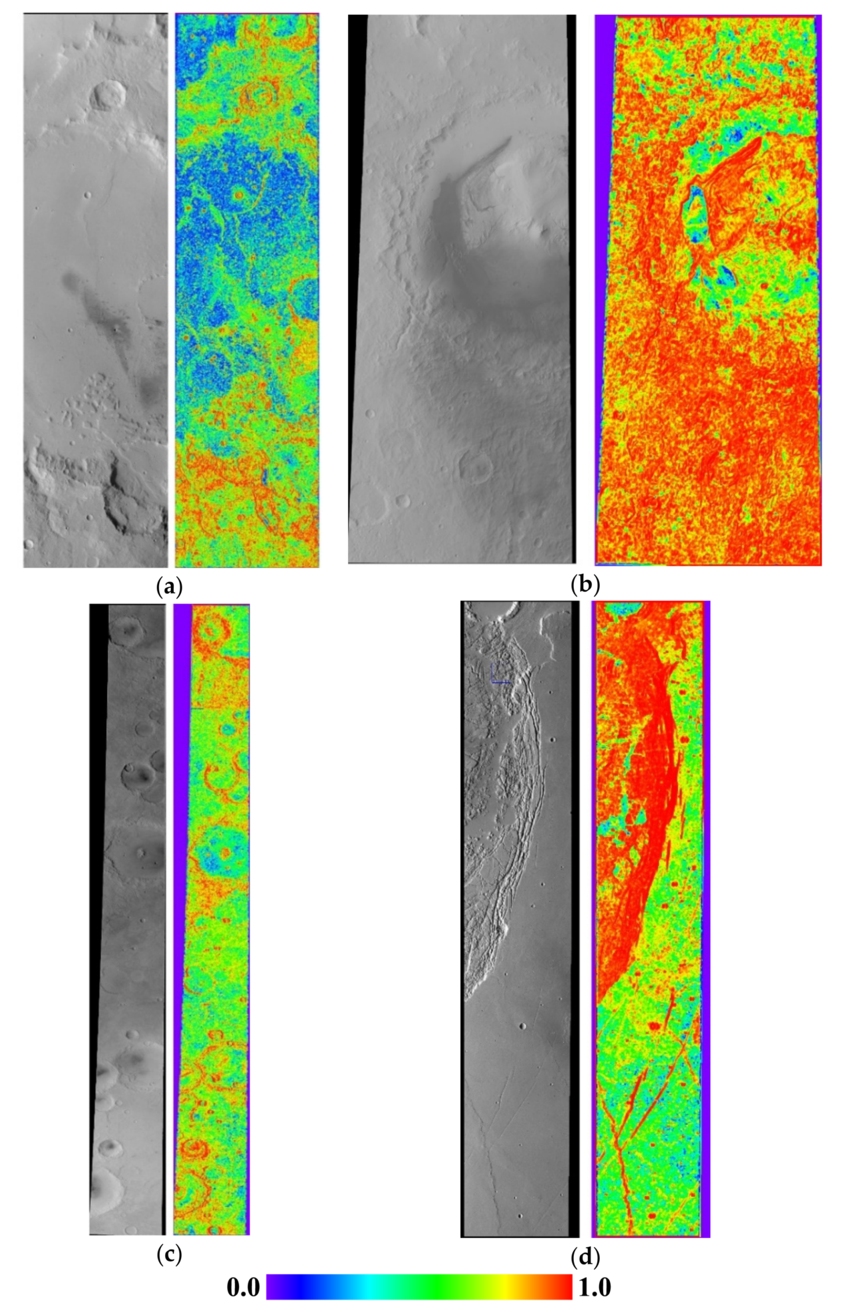
Figure 13.
The thinned conjugate points for orbit 5124 at the original image resolution level. (a) conjugate points on orthophotos; and (b) conjugate points on the original HRSC Level-2 images. Green crosses mean matched conjugate points. Numbers are used to show the relationship between the matched points on orthophotos and the matched points on the original HRSC Level-2 images.
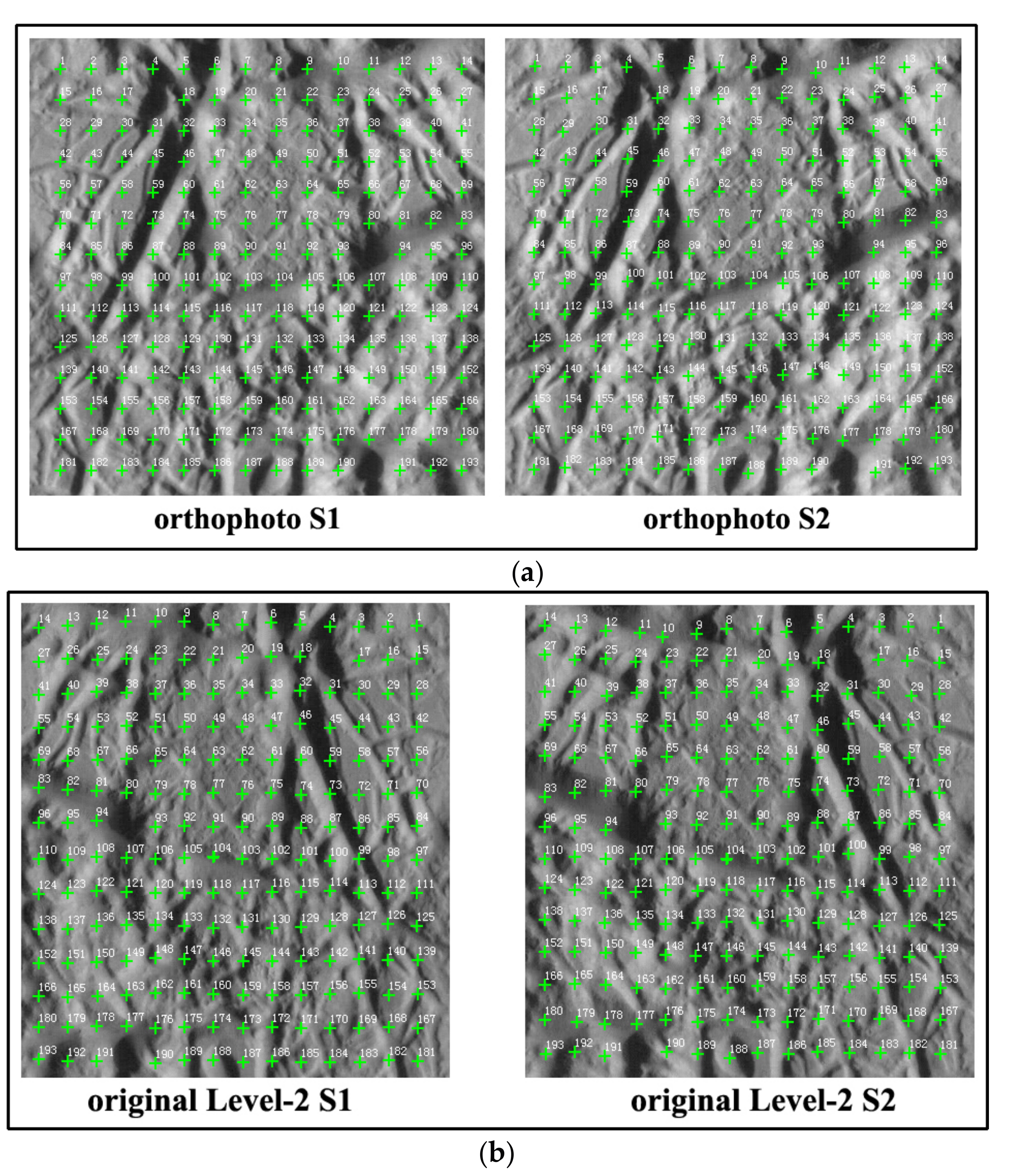
Figure 14.
Estimation accuracy for approximate positions of conjugate points at the original image resolution level: (a) scatter chart; and (b) histogram chart.
Figure 14.
Estimation accuracy for approximate positions of conjugate points at the original image resolution level: (a) scatter chart; and (b) histogram chart.

Figure 15.
Pixel coordinate displacements (PCDs) of conjugate points on the original HRSC Level-2 images.
Figure 15.
Pixel coordinate displacements (PCDs) of conjugate points on the original HRSC Level-2 images.
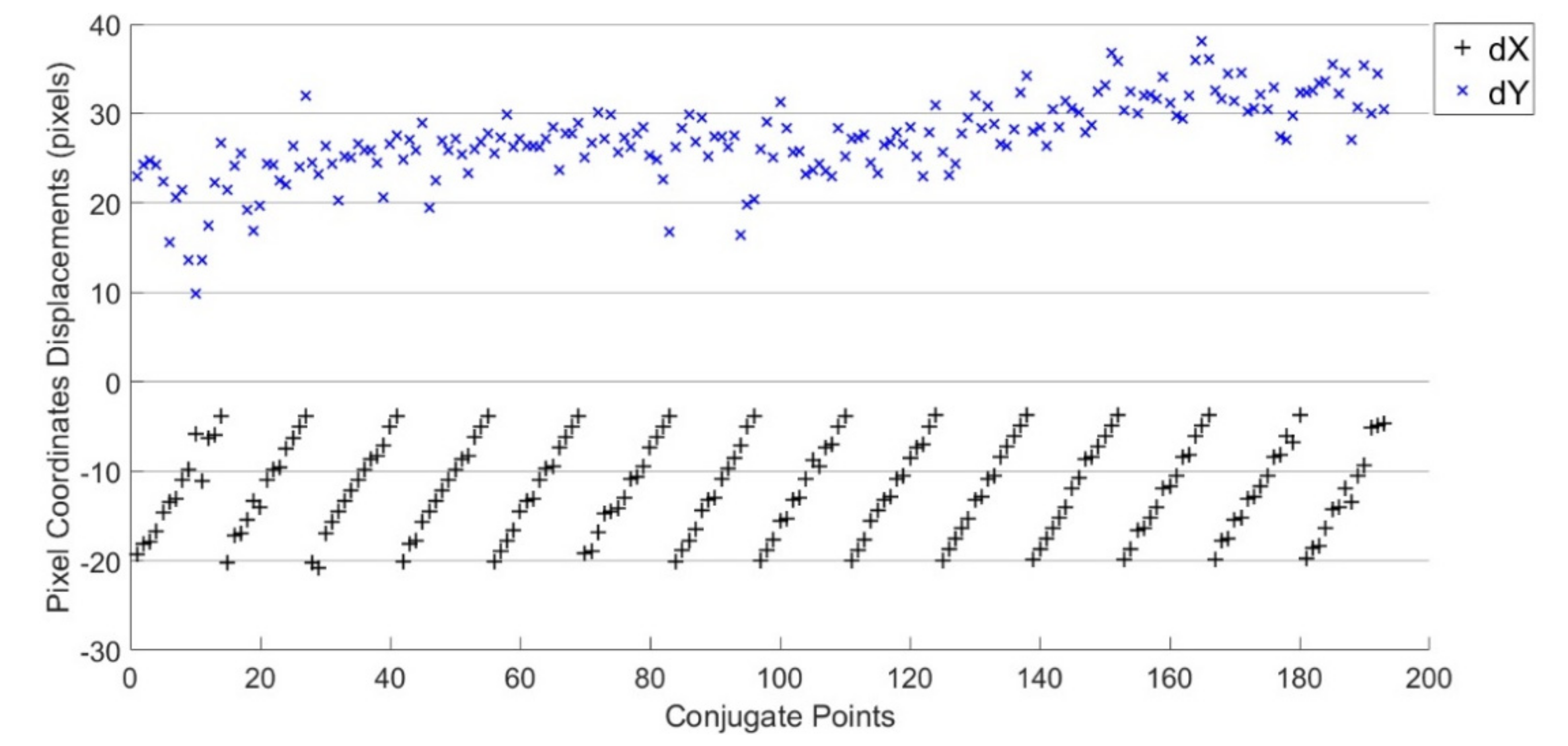
Figure 16.
DEM results and terrain profiles comparison for orbit 4165: (a) digital orthophoto map (DOM) and DEM results; and (b) terrain profiles comparison between the generated DEM and the HRSC Level-4 DEM.
Figure 16.
DEM results and terrain profiles comparison for orbit 4165: (a) digital orthophoto map (DOM) and DEM results; and (b) terrain profiles comparison between the generated DEM and the HRSC Level-4 DEM.
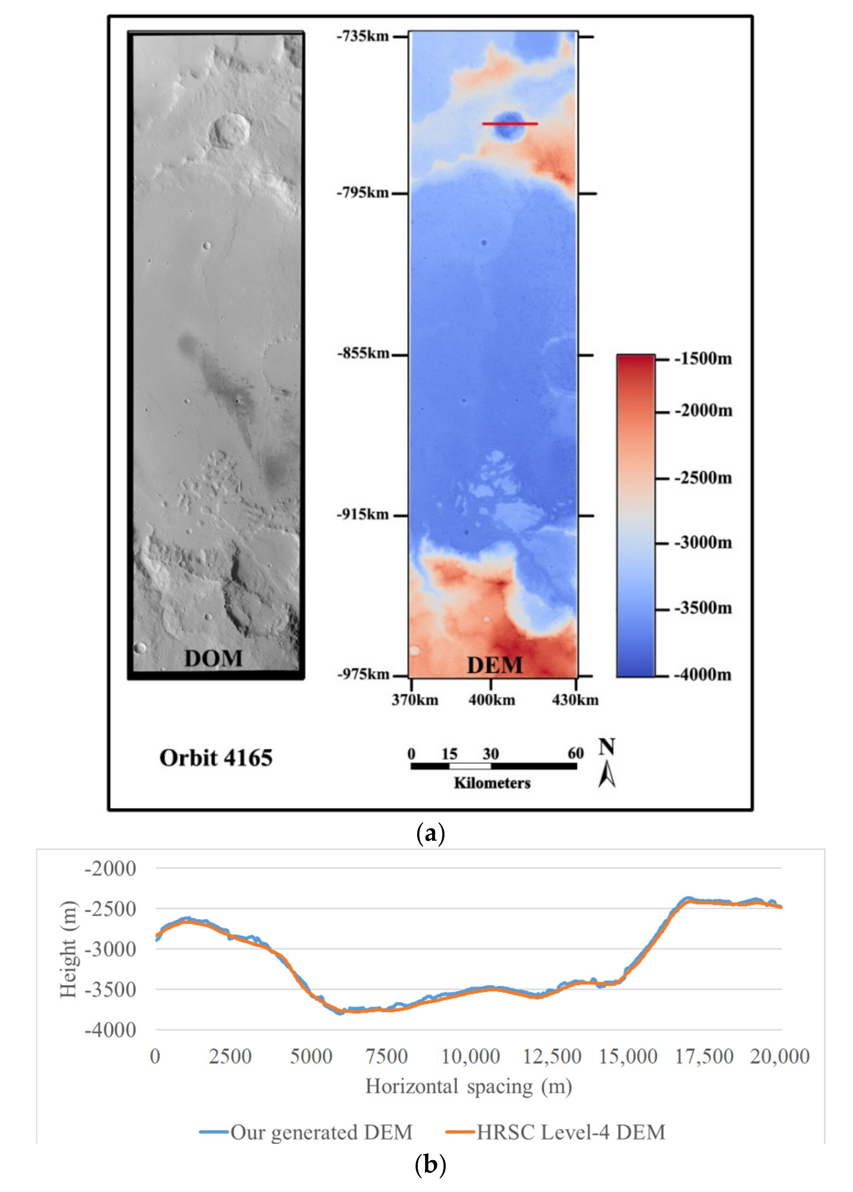
Figure 17.
DEM results and terrain profile comparison for orbit 5273: (a) DOM and DEM results; and (b) terrain profile comparison between the generated DEM and the HRSC Level-4 DEM.
Figure 17.
DEM results and terrain profile comparison for orbit 5273: (a) DOM and DEM results; and (b) terrain profile comparison between the generated DEM and the HRSC Level-4 DEM.
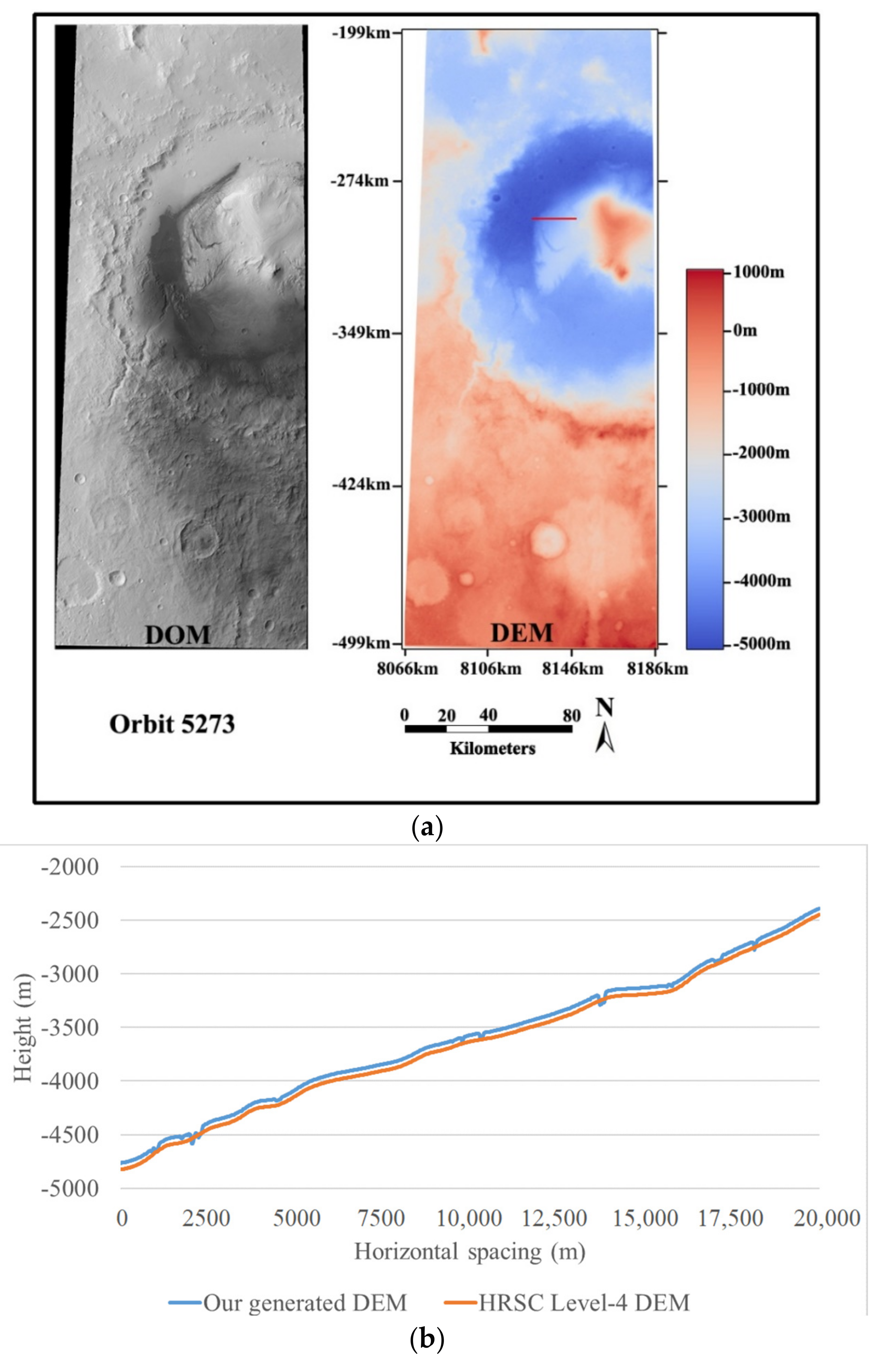
Figure 18.
DEM results and terrain profiles comparison for orbit 4235: (a) DOM and DEM results; and (b) Terrain profile comparison between the generated DEM and the HRSC Level-4 DEM.
Figure 18.
DEM results and terrain profiles comparison for orbit 4235: (a) DOM and DEM results; and (b) Terrain profile comparison between the generated DEM and the HRSC Level-4 DEM.

Figure 19.
DEM results and terrain profiles comparison for orbit 5124: (a) DOM and DEM results; and (b) Terrain profile comparison between the generated DEM and the HRSC Level-4 DEM.
Figure 19.
DEM results and terrain profiles comparison for orbit 5124: (a) DOM and DEM results; and (b) Terrain profile comparison between the generated DEM and the HRSC Level-4 DEM.
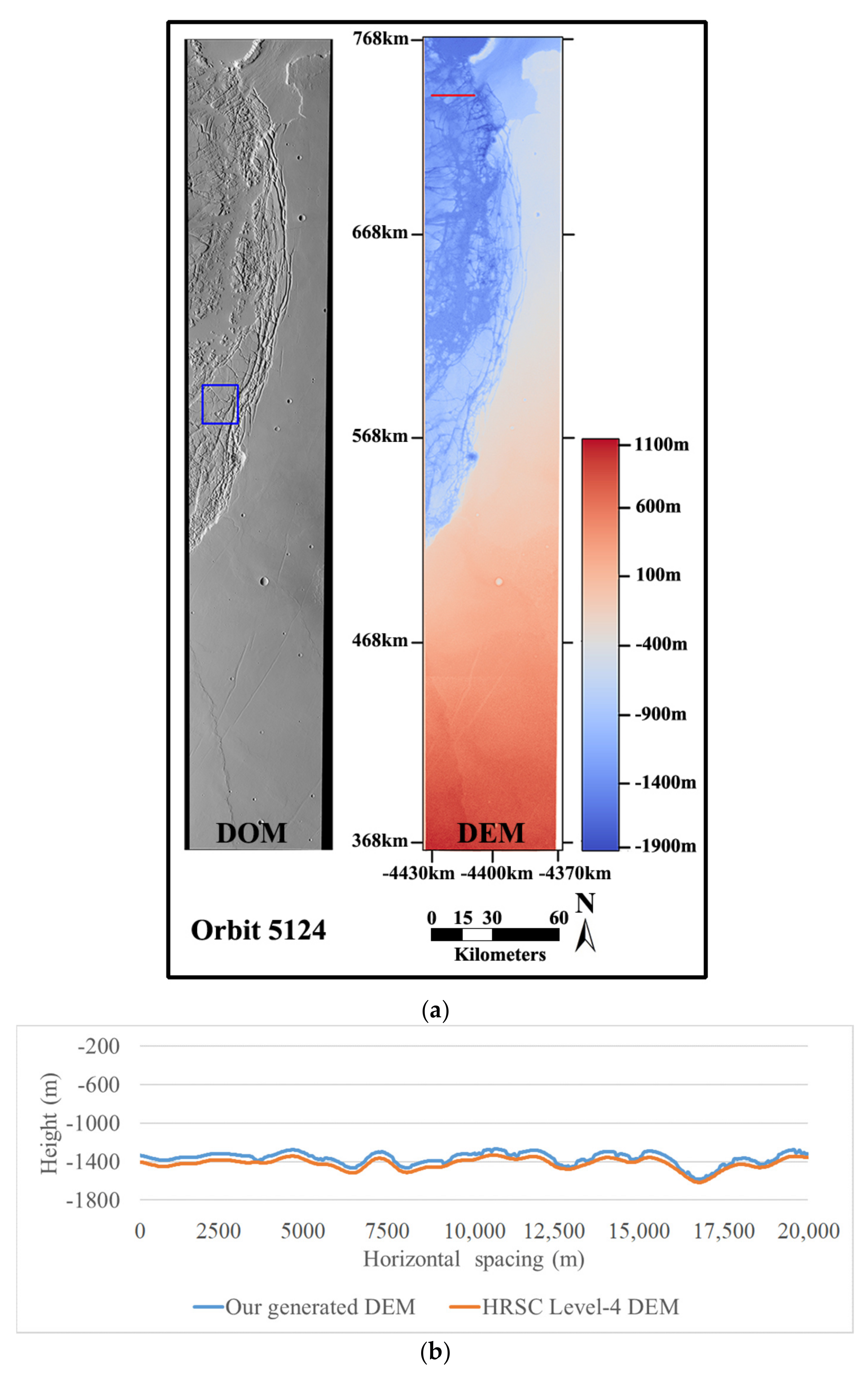
Figure 20.
Visual comparison for the generated DEM, HRSC Level-4 DEM, and MOLA DEM.


Table 1.
The calibrated camera geometric parameters for HRSC. MEX: Mars Express.
| Instrument Name | Focal Length (mm) | Boresight Sample (Pixels) |
|---|---|---|
| MEX_HRSC_S2 | 174.80 | 2588.7635 |
| MEX_HRSC_RED | 174.61 | 2585.3891 |
| MEX_HRSC_P2 | 174.74 | 2589.3140 |
| MEX_HRSC_BLUE | 175.01 | 2602.0075 |
| MEX_HRSC_NADIR | 175.01 | 2597.3376 |
| MEX_HRSC_GREEN | 175.23 | 2598.8432 |
| MEX_HRSC_P1 | 174.80 | 2597.1421 |
| MEX_HRSC_IR | 174.82 | 2595.9317 |
| MEX_HRSC_S1 | 174.87 | 2588.7635 |
Table 2.
Line exposure duration of the HRSC linear pushbroom imagery for orbit 5273. ET: emphasis time.
Table 2.
Line exposure duration of the HRSC linear pushbroom imagery for orbit 5273. ET: emphasis time.
| ET Time (s) | Line Exposure Duration (s) | Line Start |
|---|---|---|
| 255818927.127810 | 0.005013 | 1 |
| 255818938.197460 | 0.005120 | 2209 |
| 255818950.649500 | 0.005227 | 4641 |
| 255818962.691930 | 0.005333 | 6945 |
| 255818974.638750 | 0.005440 | 9185 |
| 255818986.128180 | 0.005547 | 11,297 |
| 255818997.487880 | 0.005653 | 13,345 |
| 255819008.704190 | 0.005760 | 15,329 |
| 255819019.394850 | 0.005867 | 17,185 |
Table 3.
Performance evaluation of the fast back-projection algorithm using 1 million points. Maximum errors: the maximum displacements between the calculated image points and the known ones; CT: computation time; ISI: image space iteration.
Table 3.
Performance evaluation of the fast back-projection algorithm using 1 million points. Maximum errors: the maximum displacements between the calculated image points and the known ones; CT: computation time; ISI: image space iteration.
| Channel | Traditional ISI Algorithm | Fast Back-Projection Algorithm | Speed-Up Ratio | ||||
|---|---|---|---|---|---|---|---|
| Maximum Errors (Pixels) | Number of Iterations | CT1 (ms) | Maximum Errors (pixels) | Number of Iterations | CT2 (ms) | CT1/CT2 | |
| S1 | 0.00087 | 12~15 | 16,399 | 0.00086 | 3~7 | 832 | 19.71 |
| S2 | 0.00090 | 12~15 | 16,407 | 0.00093 | 3~7 | 844 | 19.44 |
Table 4.
Matching strategies comparison between the proposed method and the HRSC team’s method.
| Matching Strategies | The Proposed Method | HRSC Team’s Method |
|---|---|---|
| is matching performed on orthophotos? | Yes | Yes |
| is area based image matching used? | Yes | Yes |
| is multi-view image matching used? | No | Yes |
| is pixel-level image matching used? | Yes | No |
| geometric constraints | image rectification | quasi-epipolar line |
| back-projection method | a fast back-projection method | not presented in detail |
Table 5.
Basic information on the experimental datasets. GSD: ground sample distance.
| Orbit Number | Date and Time | GSD (m/Pixel) | ScanLines | Incidence Angle | Emission Angle | Matching Time (Hour) |
|---|---|---|---|---|---|---|
| 4165 | 3 April 2007 (22:34:32—22:36:29) | 12.8 | S1: 5176 × 22000 S2: 5176 × 21920 | S1: 64.87° S2: 64.67° | S1: 20.35° S2: 21.12° | 2.58 |
| 5273 | 9 February 2008 (08:47:41—08:51:39) | 23.1 | S1: 5176 × 18544 S2: 5176 × 19184 | S1: 50.95° S2: 51.39° | S1: 21.74° S2: 23.13° | 1.96 |
| 4235 | 23 April 2007 (12:51:12—12:55:26) | 25.7 | S1: 2584 × 32672 S2: 2584 × 32920 | S1: 49.93° S2: 49.75° | S1: 20.77° S2: 21.55° | 1.85 |
| 5124 | 28 December 2007 (21:14:42—21:17:28) | 27.5 | S1: 2584 × 16976 S2: 2584 × 16816 | S1: 68.65° S2: 68.89° | S1: 20.58° S2: 21.11° | 0.89 |
Table 6.
The height displacements between the generated DEM and the HRSC Level-4 DEM. RMSE: root mean square errors; GSD: ground sample distance.
Table 6.
The height displacements between the generated DEM and the HRSC Level-4 DEM. RMSE: root mean square errors; GSD: ground sample distance.
| Orbit Number | Height Displacements (m) | Height Displacements in GSD (Pixels) | ||||
|---|---|---|---|---|---|---|
| Maximum Value | Mean Value | RMSE | Maximum Value | Mean Value | RMSE | |
| 4165 | 81.6 | 25.4 | 31.3 | 6.3 | 2.0 | 2.4 |
| 5273 | 76.3 | 30.5 | 34.5 | 3.1 | 1.2 | 1.4 |
| 4235 | 93.8 | 25.1 | 30.2 | 3.8 | 1.0 | 1.2 |
| 5124 | 79.2 | 40.9 | 28.6 | 3.2 | 1.6 | 1.1 |
© 2017 by the authors. Licensee MDPI, Basel, Switzerland. This article is an open access article distributed under the terms and conditions of the Creative Commons Attribution (CC BY) license (http://creativecommons.org/licenses/by/4.0/).
Share and Cite
MDPI and ACS Style
Geng, X.; Xu, Q.; Xing, S.; Lan, C.; Xu, J. A Novel Pixel-Level Image Matching Method for Mars Express HRSC Linear Pushbroom Imagery Using Approximate Orthophotos. Remote Sens. 2017, 9, 1262. https://doi.org/10.3390/rs9121262
AMA Style
Geng X, Xu Q, Xing S, Lan C, Xu J. A Novel Pixel-Level Image Matching Method for Mars Express HRSC Linear Pushbroom Imagery Using Approximate Orthophotos. Remote Sensing. 2017; 9(12):1262. https://doi.org/10.3390/rs9121262
Chicago/Turabian StyleGeng, Xun, Qing Xu, Shuai Xing, Chaozhen Lan, and Junyi Xu. 2017. "A Novel Pixel-Level Image Matching Method for Mars Express HRSC Linear Pushbroom Imagery Using Approximate Orthophotos" Remote Sensing 9, no. 12: 1262. https://doi.org/10.3390/rs9121262
Note that from the first issue of 2016, this journal uses article numbers instead of page numbers. See further details here.