Mapping Plastic-Mulched Farmland with C-Band Full Polarization SAR Remote Sensing Data

1
Key Laboratory of Grassland Resources, Ministry of Education, P.R. China/Key Laboratory of Forage Cultivation, Processing and High Efficient Utilization, Ministry of Agriculture, P.R. China, College of Grassland, Resources and Environment, Inner Mongolia Agricultural University, No. 29, Erdos Dongjie, Saihan District, Hohhot 010011, China
2
Key Laboratory of Agricultural Remote Sensing, Ministry of Agriculture, P.R. China (AGRIRS)/Institute of Agricultural Resources and Regional Planning, Chinese Academy of Agricultural Sciences, No. 12, Zhongguancun Nan Dajie, Haidian District, Beijing 100081, China
*
Author to whom correspondence should be addressed.
Remote Sens. 2017, 9(12), 1264; https://doi.org/10.3390/rs9121264
Submission received: 26 September 2017
/
Revised: 3 December 2017
/
Accepted: 4 December 2017
/
Published: 6 December 2017
(This article belongs to the Section Remote Sensing in Agriculture and Vegetation)
Abstract
:Plastic mulching is an important technology in agricultural production both in China and the rest of the world. In spite of its benefit of increasing crop yields, the booming expansion of the plastic mulching area has been changing the landscape patterns and affecting the environment. Accurate and effective mapping of Plastic-Mulched Farmland (PMF) can provide useful information for leveraging its advantages and disadvantages. However, mapping the PMF with remote sensing is still challenging owing to its varying spectral characteristics with the crop growth and geographic spatial division. In this paper, we investigated the potential of Radarsat-2 data for mapping PMF. We obtained the backscattering intensity of different polarizations and multiple polarimetric decomposition descriptors. These remotely-sensed information was used as input features for Random Forest (RF) and Support Vector Machine (SVM) classifiers. The results indicated that the features from Radarsat-2 data have great potential for mapping PMF. The overall accuracies of PMF mapping with Radarsat-2 data were close to 75%. Although the classification accuracy with the back-scattering intensity information alone was relatively lower owing to the inherent speckle noise in SAR data, it has been improved significantly by introducing the polarimetric decomposition descriptors. The accuracy was nearly 75%. In addition, the features derived from the Entropy/Anisotropy/Alpha (H/A/Alpha) polarimetric decomposition, such as Alpha, entropy, and so on, made a greater contribution to PMF mapping than the Freeman decomposition, Krogager decomposition and the Yamaguchi4 decomposition. The performances of different classifiers were also compared. In this study, the RF classifier performed better than the SVM classifier. However, it is expected that the classification accuracy of PMF with SAR remote sensing data can be improved by combining SAR remote sensing data with optical remote sensing data.
1. Introduction
The practice of plastic mulching has changed agricultural production radically all over the world [1]. Plastic mulching is a practice of tightly covering plastic film over the soil surface to promote crop growth and increase crop yield. Plastic mulching can protect crops from unfavorable growing conditions (droughts, coldness, heat, weeds and/or pests) and increase the crop yields. On the other hand, large-scale projects using this technique are expected to put further pressure on the environment, such as “white pollution”, soil degradation [2,3] and the alternation of the material and energy exchange [4]. The environmental problems caused by Plastic-Mulched Farmland (PMF) expansion have been exacerbated in recent years [2,5], creating a pressing demand to optimize the use of plastic mulching. Thus, accurate mapping of PMF (obtaining the information about spatial pattern and amount of PMF according its specific signature via remote sensing technology) at a local or regional scale is needed for decision-makers and researchers. It is well-known that remote sensing is a technique to obtain the up-to-date information effectively over a large region and across long time span [6]. During the recent decades, mapping land cover types with remote sensing data has drawn increasing attention and obtained many valuable results. The extraction of the specific land cover type, such as a water body [7,8], impervious surface [9], snow and ice [10,11], vegetation cover classification [12], has raised interests greatly.
In recent years, increasing attention has been paid to map the plasticulture landscape with remote sensing. But most of the researches were on mapping plastic greenhouses rather than PMF. The topic is relevant to passive remote sensing data with which plasticulture has been mapped by two main approaches: pixel-based and object-based classifiers. For example, Agüera et al. proposed a pixel-based approach for mapping plastic greenhouses using texture features from QuickBird images [13,14]. Carvajal et al. mapped plastic greenhouse using QuickBird and IKONOS images [15]. Arcidiacono et al. presented an improved pixel-based approach for mapping crop-shelter coverage by using high-resolution satellite images [16,17]. Koc-San evaluated the performance of different pixel-based classifiers for differentiating glass and plastic greenhouses using WorldView-2 images [18]. Recently, studies have developed an object-based approach for mapping plastic greenhouses using high spatial resolution images [19,20,21]. All these studies mostly used high spatial resolution remote sensing images. Although the high spatial resolution images provided data for mapping plastic greenhouses efficiently in a fixed region, their application will be limited by a large spatial extent, large data storage and costly data procurement. More recently, studies developed an object-based approach for mapping plastic greenhouses using medium spatial resolution images [22,23,24]. In addition, Levin et al. studied the spectral properties of various plastic polyethylene sheets using a field spectrometer and detected three major absorption features around 1218 nm, 1732 nm and 2313 nm [25].
However, the spatial pattern of PMF is wider than that of plastic greenhouses in China, and the spectral response of PMF is changing more quickly than that of plastic greenhouses. Mapping PMF with remote sensing began in the last few years. Lu et al. presented a decision-tree classifier for mapping PMF in Xinjiang, China, with Landsat-5 images and obtained ideal results [5]. However, plastic mulching in China was applied during the sowing stage, and the spectral reflectance of the PMF is influenced by the developing crops. Therefore, the detectable period of PMF is very short (one week to two weeks). Additionally, the long revisiting of the Landsat satellite limits its usage for PMF mapping, as it is difficult to capture the changing characteristic of PMF with crop phenology. For this, they, afterwards, performed an index-based threshold method for PMF mapping using a time series MODIS-NDVI (Moderate-resolution Imaging Spectrometer-Normalized Difference Vegetation Index) [26] and also obtained an acceptable result. These two methods are limited by several factors: (1) the regional differences of PMF will limit the performance when applied to other regions; (2) when using low resolution imagery, some smaller PMF are lost, and mixed pixel phenomenon may become more serious, because of the small patch and fragmented agricultural land use patterns in China. Therefore, a comprehensive consideration of these issues is required for improving the robustness of the PMF mapping approach. For this, Hasituya et al. mapped the PMF by using multiple features, including spectral features, textural features, index features, thermal features and temporal features generated from the Landsat-8 imagery [27,28]. The results pointed out that the multi-temporal features perform better than the single temporal features; and the spectral features and index features are better than the textural features and thermal features. However, the textural features generated from the high resolution data of GF-1 (GaoFen-1, the first satellite in the Chinese High-resolution Earth Observation System (CHEOS)) perform better than its spectral features for PMF mapping [29]. In addition, Lanorte et al. estimated and mapped agricultural plastic waste by using satellite images and obtained ideal results [30]. By reviewing the published literature, we found that these studies regarding mapping of PMF with remote sensing are limited, and all used optical remote sensing data. Additionally, the usage of microwave remote sensing data, especially Synthetic Aperture Radar (SAR) data, is rather absent.
The approaches used in specific object mapping/detecting are generally divided into: (1) supervised and unsupervised classifiers; (2) sub-pixel based, per-pixel based and object-based classifiers according to the basic operating unit; (3) single-classifier and ensemble classifier algorithms based on the number of classifiers; and (4) index-based automatic extraction methods. The methods for mapping plastic greenhouses include conventional supervised classification, object-based methods, machine learning classifiers, index-based threshold methods, and so on. However, the methods for mapping PMF mainly include the Index-based Threshold methods, Decision Tree classifiers, Support Vector Machine (SVM) classifiers, Random Forest (RF) classifiers, and so on. The relevant studies reported that the machine learning algorithm is superior to the other supervised classifiers.
Compared with optical and thermal infrared remote sensing, SAR remote sensing has several advantages regarding the capability of all-weather and all-time observations, the ability to penetrate cloud cover and record the information about the structure, surface roughness, shape and dielectrics of the object [31]. SAR data contain scattering information that can reveal the scattering mechanism of the objects. Therefore, SAR remote sensing plays a very important role in target recognition, classification and parameter inversion. With the rapid development over half a century, the SAR system has now formed a multi-band, multi-mode, multi-polarization and multi-resolution imaging technology system. The application domains of SAR remote sensing are also expanding from terrain mapping, land cover classification [32,33], crop type identifying [34,35,36], crop phenology monitoring [37], inversion of soil moisture [38] and estimation of biomass and crop yield to snow cover monitoring, flooding mapping [39], coastline monitoring [40,41] and sea surface environmental monitoring [42,43].
Polarimetric decomposition of SAR data is a technique for separating the complex scattering mechanism of an object. Polarimetric decomposition can simplify the complex scattering mechanism as several kinds of simple scattering mechanisms, which are related to the physical structure of targets, and can thus be used to classify land cover types [33]. Thereby, we can analyze the scattering characteristics of the object and identify this object based on a simple scattering mechanism. Polarimetric decomposition can be classified into coherent decomposition based on a scattering matrix and non-coherent decomposition based on a covariance matrix or coherent matrix. Coherent decomposition includes Krogager decomposition, Huynen decomposition, Cameron decomposition, and so on. The non-coherent decomposition includes Freeman decomposition (three-component or two-component), Yamaguchi4 decomposition and Entropy/Anisotropy/Alpha (H/A/Alpha) decomposition [44]. By these polarimetric decomposition methods, we can quantitatively express single scattering, double bounce scattering and random scattering intensity in the SAR scattering mechanism.
Plastic mulching changes the surface roughness and soil moisture. Therefore, the backscattering and polarimetric decomposition characteristics of the PMF are different from those of other objects theoretically. To provide more possibilities for PMF mapping with remote sensing, the current study provided new insights into the use of high resolution C-band SAR data for PMF mapping and evaluated the use of polarimetric decomposition of SAR data, which can be acquired independent of local weather and provide an information source complementary to optical remote sensing systems. The proposed methodology was based on the integration of backscattering intensity, polarimetric decomposition and machine learning algorithms. The main objectives of this study are (1) to examine the backscattering characteristic of PMF; (2) to mine the effective features of SAR data for PMF mapping, including the polarimetric decomposition features; and (3) to compare the performance of two different machine learning algorithms, namely RF and SVM.
2. Study Areas and Data
2.1. Study Areas
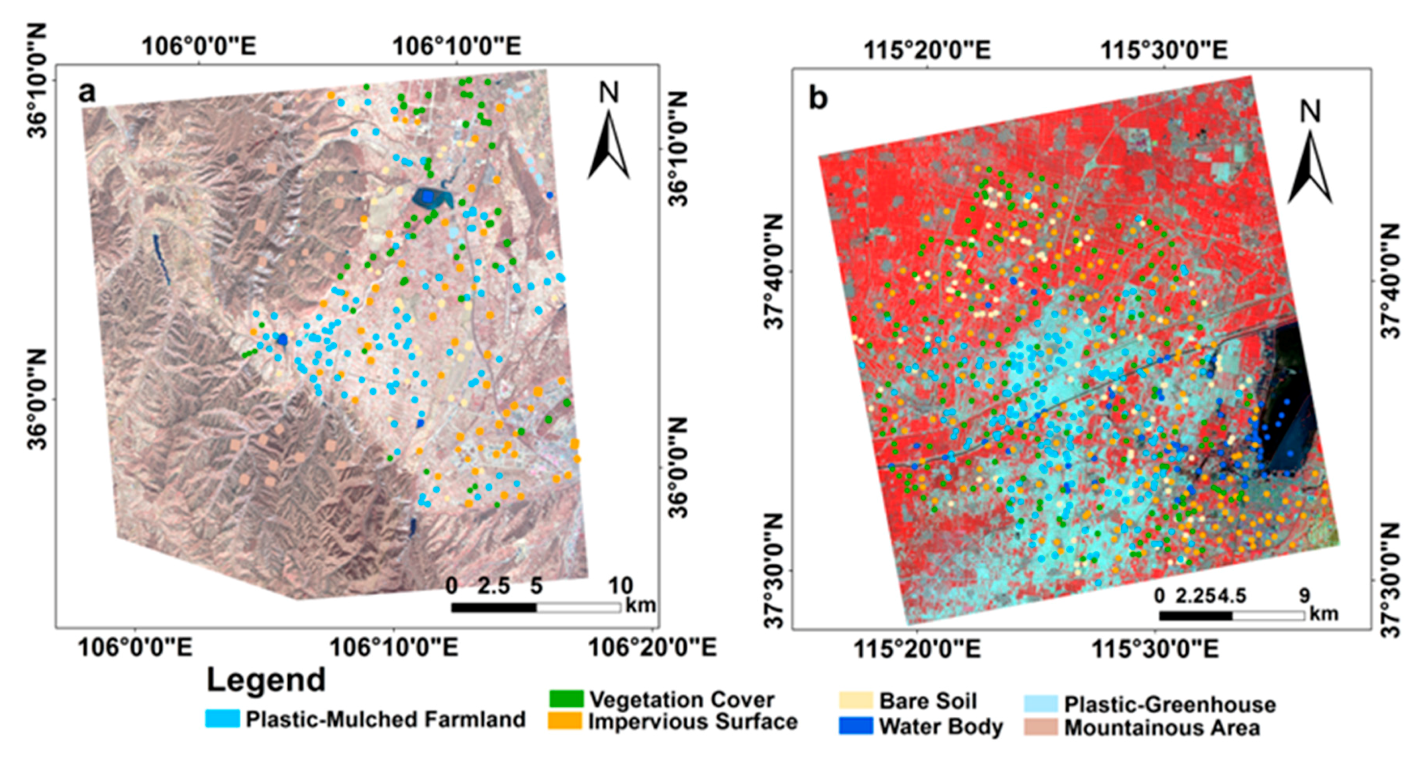
In this study, two typical PMF areas (Figure 1) with different plastic-mulching modes were selected as the experimental region.
The first study area is Jizhou, Hebei Province, China. This is one of the main grain producing areas in the North China Plain [45]. This region is in a temperate monsoon climate zone with a hot and rainy summer that favors crop development. The main crops in this area include winter wheat, cotton, corn and vegetables. The cotton fields are the dominant plastic-mulched crops in this area. White plastic mulching has been utilized in Jizhou generally. Other land cover/use types consist of woodland, grassland, water body and impervious surface.
The second study area is Guyuan, Ningxia Hui Autonomous Region, China. This region is located in a temperate semi-arid climate zone. Irrigation is needed to facilitate crop growth and development in this region. Plastic mulching has been widely used here for water-saving and yield-increasing. The plastic-mulched crops include corn, winter wheat and vegetables. It was observed that early spring and autumn are the main periods for mulching. White plastic mulching has been utilized in Guyuan, as well.
2.2. Data
Data used in this study include two scenes of Radarsat-2 images, four scenes of GF-1 images and the field survey data.
2.2.1. Remote Sensing Data and Preprocessing
Radarsat-2, the C-band SAR satellite, encompass powerful and significant advancements in satellite techniques, one of which is the multi-polarimetric mode [31,46,47]. It can transmit both the vertical (V) and horizontal (H) polarimetry. The detailed parameters of Radarsat-2 data are presented in Table 1.
The Radarsat-2 data of the two study areas were preprocessed firstly, including multi-looking, radiation calibration, filtering, geometric correction, and so on, using the SAR Toolbox software (NEST) from the European Space Agency (ESA). The original data were converted into backscattering coefficient data by radiometric calibration. We used the Lee-refined filtering method to remove the spot noise in the 7 × 7 filtering window. Finally, the geometric correction was carried out, and the images were resampled to 8-m resolution and output in dB format.
GF-1 images were collected for the reference sample collection. GF-1 satellite has one panchromatic band with 2-m resolution and four multispectral bands (blue, green, red and near infrared band) with 8-m resolution. The GF-1 data used in this study contain two scenes of images taken on 5 May 2015 for Jizhou and two scenes of images taken on 8 April 2015 for Guyuan. The radiometric calibration and atmospheric correction were carried out for GF-1 multispectral data in ENVI software. The multispectral images and panchromatic were then fused to 2-m spatial resolution imagery using a Gram–Schmidt pan sharpening algorithm for collecting the pure pixel samples.
2.2.2. Field Survey Data
Field surveys were carried out during 25–30 April 2015 and 23–26 June 2015 in Jizhou and Guyuan, respectively, to gather the field reference samples of land cover types. Random sampling was used to avoid missing the samples of rare distributed land cover types and to ensure the uniformity and representativeness of the collected samples across the study area and land cover types. In the field, we used GPS for positioning the samples and labeling the name of land cover types. Because some land cover types was rare distributed, we have not strictly defined the distance between samples. However, we try to avoid collecting samples that are too close. The land cover types and the collected samples in this study are summarized in Table 2. After collecting field point samples, we digitized the polygon samples based on the location of field point samples in the high spatial resolution GF-1 satellite images. The samples were enlarged to polygon samples with a size of 60 m × 60 m. As shown in Table 2, a total of 708 samples were collected for Jizhou, and 653 samples were collected for Guyuan. The samples of each study area were equally divided into two groups: training samples and test samples. The first group was used both to analyze the separability of land cover types and to train the machine learning classifiers, while the second group was used to assess the classification accuracy. The spatial distribution of the samples in the two study areas is displayed in Figure 2.
3. Methodology
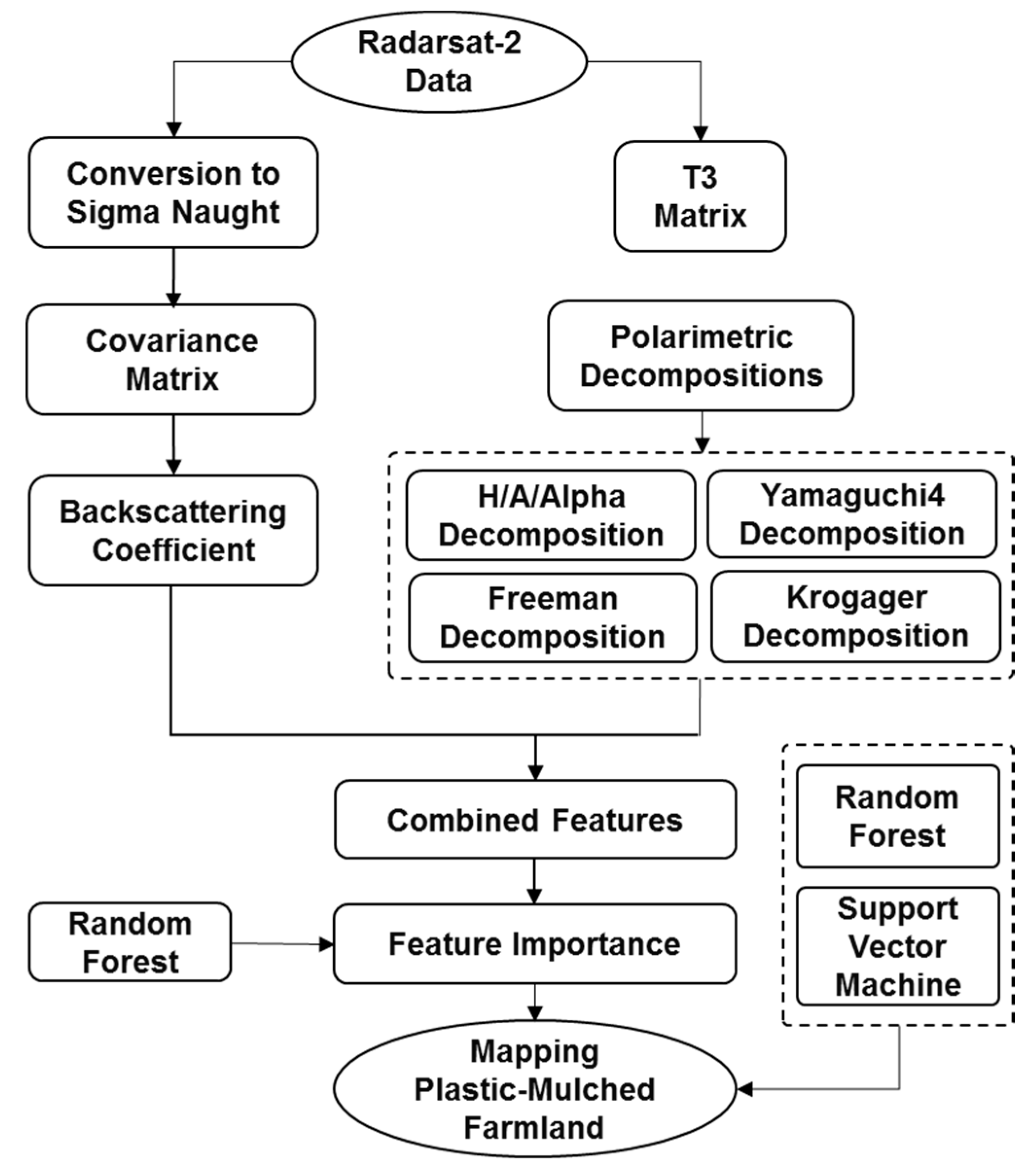
The workflow of this study is displayed in Figure 3. The preprocessing algorithms of Radarsat-2 data, the polarimetric decomposition algorithms and the machine learning algorithms were used in this study. To begin with, the Radarsat-2 data were calibrated, filtered (using the 7 × 7 refined Lee filter) and geo-corrected. Then, the backscattering intensity was obtained, and the coherency matrix T3 was extracted from the S matrix using PolSARpro software [48]. The coherency matrix T3 contained all the polarimetric information. Then, the Krogager decomposition, Freeman decomposition, Yamaguchi4 decomposition and H/A/Alpha decomposition algorithms were applied to extract a total number of 17 different polarimetric decomposition descriptors. Next, the backscattering intensity and polarimetric decomposition features were combined to form a multichannel image including a total number of 24 features for mapping PMF. After this, two machine learning algorithms, the Random Forest (RF) algorithm and the Support Vector Machine (SVM) algorithm, were used to map the PMF in the two selected study areas. Additionally, RF was also used to assess feature importance.
3.1. Separability Analysis
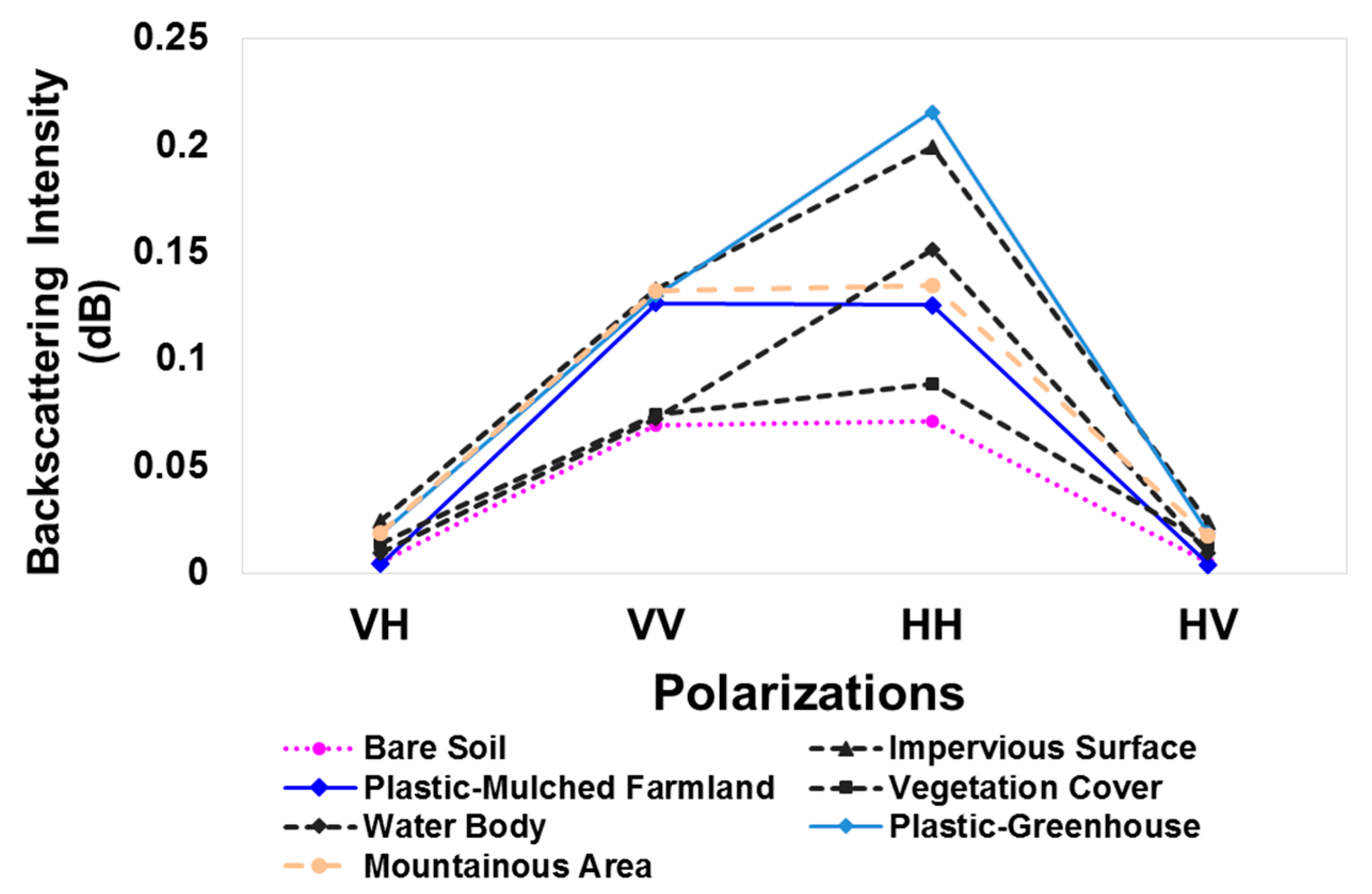
The mean values of the backscattering coefficient of different polarization were extracted from preprocessed images (Figure 4 for Jizhou and Figure 5 for Guyuan). In Figure 4, it can be seen that the backscattering intensities of PMF and bare soil in Jizhou were very similar. In particular, the mean values of the cross-polarization (HV, VH) were substantially overlapped with each other. This situation on the cross-polarization (VH, HV) was slightly better than co-polarization (HH, VV), but the separation was still poor. However, the separability between PMF and the impervious surface was better. In Figure 5, it can be seen that the backscattering intensity of PMF in Guyuan on cross-polarization (VH, HV) was poorly separated from other land cover types. Additionally, the separation on the co-polarization (HH, VV) was better than cross-polarization, while the separation on HH was better than VV polarization.
3.2. Polarimetric Decomposition
The full polarization SAR data can represent the information about land surface geometrical structure, direction, shape, humidity and surface roughness. The inclusion of SAR polarization information allows us to discriminate the different scattering mechanisms of different land cover types, so as to improve the accuracy and quality of classification significantly [33]. Polarimetric decomposition is a technique that separates a signal received by the radar into a combination of the several electromagnetic scattering responses, which can be used to extract the information of different land cover types in images. Several types of polarimetric decomposition algorithms were used successfully in the land cover classification. The H/A/Alpha decomposition, Freeman decomposition, Yamaguchi4 decomposition and Krogager decomposition algorithms were tested in this study. All the polarimetric decomposition algorithms were performed in the PolSARPro-4.2 software [48], and the corresponding polarimetric descriptors were extracted for mapping support (Table 3).
The H/A/Alpha decomposition algorithm was developed by Cloude and Pottier in 1997 for extracting polarimetric decomposition descriptors from SAR data based on the coherency matrix T3 extracted from the S matrix [33]. The H/A/Alpha decomposition generated three main parameters: Alpha (α), entropy (H) and Anisotropy (A). Among them, α changes from 0° to 90°, which represents different physical scattering mechanisms. When α = 0°, the scattering mechanism is dominated by surface scattering. When α changes from 0° to 45°, the scattering mechanism is represented by dipole scattering. When α changes from 45° to 90°, the scattering mechanism is indicated by dihedral angle scattering. When α = 90°, it represents dihedral or helix scattering. Entropy (H) represents the randomness of scattering. The H value ranges from 0–1. When H = 0, it represents isotropic scattering at a complete polarization state. When H = 1, it represents anisotropic scattering at a complete randomness scattering, and no polarization information can be obtained in this case. Therefore, when H ranges from 0–1, the scattering mechanism is changed from complete polarization to complete random scattering. The Anisotropy (A) is a supplement to the entropy. When H is very high or low, A will not provide effective supplemental information. A is the source of further identification [49,50,51]. Besides, the high entropy multiple scattering parameters (Combination_1mH1mA), high entropy plane scattering parameters (Combination_1mHA), low entropy multiple scattering parameters (Combination_H1mA) and low entropy plane scattering parameters (Combination_HA) were extracted from H/Alpha/A decomposition and used in this study.
The Krogager decomposition is a coherent decomposition method for decomposing the target signal into three components of helix (Kh), di-plane (Kd) and sphere (Ks) using a scattering matrix [52]. Ks is the contribution of the decomposed surface scattering component. Kh is the contribution of the decomposed helix scattering component. Kd is the contribution of the decomposed di-plane scattering component.
The Freeman decomposition is an incoherent decomposition method for decomposing scattering mechanism of SAR observations into surface scattering, double-bounce scattering and volume scattering, which can provide features for distinguishing different surface cover types [50].
3.3. Machine Learning Algorithms and Accuracy Assessment
In this study, we used RF and SVM classifiers to map the PMF in these two study areas.
3.3.1. Random Forest
RF is an ensemble supervised classifier developed by Breiman in 2001 [55]. RF has been widely used in remote sensing classification because it is efficient to compute, robust to outliers and noise and useful for assessing variable importance [56]. In this study, the RF algorithm was used to map the PMF using features from Radarsat-2 data. Two parameters, the number of trees and the number of variables, were set beforehand. A total number of 500 trees and the square root of the input features number were set in this study.
3.3.2. Support Vector Machine
Another machine learning supervised classifier, SVM, was also used in this study based on the same features and the same samples to map PMF. The SVM uses the principle of structural risk minimization, not the empirical risk minimization [57]. The performance of SVM has been proven by many studies [58,59,60,61,62,63] using optical and SAR remote sensing data for mapping one-class land cover types or classifying the land cover/use types. We used the Radial Basis Function (RBF) kernel SVM in this study. The SVM has been parameterized to determine the regularization parameter (c) and the Gaussian RBF kernel parameter (g) before each classification. The Gaussian RBF kernel parameter (g) range was set between 0.001 and 1000 with a multiplier of 10. The regularization parameter (c) range was set between 0.001 and 1000 with a multiplier of 10. The termination criteria were about 0.1 for grid search and 0.001 for final training with 3-fold cross-validation. Afterward, we ran the SVM algorithm using the optimized value of the regularization parameter (c) and the Gaussian RBF kernel parameter (g) for mapping the PMF.
3.3.3. Accuracy Assessment
The confusion matrix was used in accuracy assessment. The confusion matrix is a widely-used approach to assess the classification accuracy of remote sensing images. In this study, the Overall Accuracy (OA) and the Kappa coefficient (K) were employed to assess the general classification efficiency, while the Producer’s Accuracy (PA) and the User’s Accuracy (UA) were employed to assess the accuracies of individual class.
The Z test was used in statistical significance testing for classification accuracies [64]. The classification accuracies of this study were further confirmed by using the Z test, which tests the statistical significance of the K statistic and significance differences of different classifications schemes.
It is satisfying to perform this test on a single error matrix and to confirm that the classification is meaningful and significantly better than a random classification. The test statistic for testing the significance of a single error matrix is expressed by Formula (1):
where K denotes the estimates of the Kappa statistic for error matrix. The Var(K) denotes the corresponding estimates of the variance of K. At the 99% confidence level, the critical value would be 2.58. Therefore, if the absolute value of the Z test statistic is greater than 2.58, the result is stable and significant.
With this test, it is also possible to compare statistically two analysis, the same analysis over time, two algorithms or even two types of imagery and to check which produces the higher accuracy. To verify the effectiveness of different feature sets and different classifiers, the Z test was performed on the pairwise error matrix of different analysis. The test statistic for testing if two independent error matrices are significantly different is expressed by Formula (2):
where K1 and K2 denote the estimates of the Kappa statistic for Error Matrices 1 and 2, respectively. The Var(K1) and Var(K2) are the corresponding estimates of the variance of K as computed from the appropriate equations. At the 99% confidence level, the critical value would be 2.58. Therefore, if the absolute value of the Z test statistic is greater than 2.58, the two analysts are significantly different.
3.4. Input Feature Selection
In this study, the RF algorithm was used to assess the features’ importance [65]. A detailed process for measuring the importance of features by RF was presented by Guan et al. [66]. We repeated the importance assessment ten times and calculated the average importance value to avoid differences across different runs. The features were ranked in descending order of their average importance, and the cumulative average importance was calculated. After that, different feature sets were developed based on the cumulative percentage of feature importance, such as the cumulative percentages of 80%, 90% and 100%, for mapping PMF.
In order to discuss the influence of the feature selection algorithm, we also used the SVM feature selection algorithm to compare the difference between RF and SVM. SVM feature selection uses a backward/forward elimination approach and selects a fixed number of top ranked features, providing the largest margin between classes for further classification. The detailed description of SVM feature selection can be found in [57]. In this study, we selected the top 10, 15 and 24 features to map the PMF in Jizhou and to compare it with RF.
4. Results
4.1. Importance of SAR Features for Mapping PMF
The RF algorithm was used to evaluate the importance of the total 24 features, which include backscattering intensity of different polarizations and the polarimetric decomposition descriptors.
Analysis of feature importance (Figure 6) suggested that the descriptors derived from the H/A/Alpha decomposition were the most important features for mapping PMF. Additionally, the descriptors generated from the Yamaguchi4 and the Freeman decomposition were found to be the next most important features, while the contribution of Krogager decomposition descriptors was the smallest. The importance order of Radarsat-2 features for mapping PMF in Jizhou was ranked as Alpha, entropy, VH, HV, C_1mH1mA, C_H1mA, C_1mHA, C_HA, Y_Odd and anisotropy. Additionally, that in Guyuan was ranked as Alpha, VH, HH, VV, HV, entropy, C_H1mA, C_1mH1mA, C_1mHA, C_HA, and so on.
In Figure 7, we display the images of the more important features for mapping PMF. It can be seen that the gray value of PMF on the images of Alpha, entropy, C_H1mA and C_HA is darker than that of other land cover types (except for water body). Additionally, the gray value of PMF is lighter than the other land cover types on the images of C_1mH1mA and C_1mHA.
4.2. Classification Accuracy of PMF with Radarsat-2 Data
The classification accuracies are displayed in Table 4. The PMF classification accuracies indicated that the best result was obtained from all available combined features in Jizhou and Guyuan. The second best results were generated from the 90% features in Jizhou and Guyuan, respectively. Additionally, the worst results was generated from the backscattering intensity of different polarizations alone.
For Jizhou, the accuracies obtained from the backscattering coefficient intensity of different polarizations (VH, HH, VV and HV) alone were relatively low. The overall accuracy, producer’s accuracy and user’s accuracy from backscattering coefficient intensity were 59.75%, 68.29% and 52.71%, respectively. However, the accuracies were improved significantly by including the descriptors derived from the different polarimetric decomposition. The highest overall, producer’s and the user’s accuracies were improved to 74.82%, 85.31% and 67.56%, respectively, by combining the backscattering coefficient intensity of different polarizations with the descriptors derived from the different polarimetric decomposition algorithms. The accuracy improvement was about 15 percentage points on average.
For Guyuan, the accuracies from the backscattering coefficient intensity of different polarizations (VH, HH, VV and HV) alone were also relatively low. The overall accuracy, the producer’s accuracy and the user’s accuracy were 56.83%, 65.43% and 49.69%, respectively. This level of accuracy cannot meet the practical application requirements generally. However, the accuracies were improved significantly by combining the backscattering coefficient intensity with the polarimetric decomposition descriptors. Additionally, the highest overall, producer’s and the user’s accuracies achieved were 64.21%, 74.49% and 51.93%, respectively. The average accuracy improvement was about 15 percentage points, as well.
We can explain the contribution of the polarimetric decomposition descriptors for mapping PMF by comparing the approaches with and without polarimetric decomposition descriptors. The overall accuracy was increased by 15.07 percentage points in Jizhou and 7.38 percentage points in Guyuan when using RF with the polarimetric decomposition descriptors in classification. Additionally, the overall accuracy was increased by 15.20 percentage points in Jizhou and 10.00 percentage points in Guyuan when using SVM with the polarimetric decomposition descriptors in classification. Furthermore, the user’s and producer’s accuracies of PMF were improved also by employing the polarimetric decomposition descriptors. The producer’s accuracies for PMF were increased by 17.02 percentage points in Jizhou and 9.06 percentage points in Guyuan when using RF with the polarimetric decomposition descriptors in classification. When using SVM, the producer’s accuracies for PMF were increased by 18.30 percentage points in Jizhou and 3.31 percentage points in Guyuan. Additionally, the user’s accuracies for PMF were increased by 14.02 percentage points in Jizhou and 2.24 percentage points in Guyuan when using RF with the polarimetric decomposition descriptors in classification. When using SVM, the user’s accuracies for PMF were increased by 15.71 percentage points in Jizhou and 1.60 percentage points in Guyuan. From these accuracy improvements, we can confirm that the polarimetric decomposition descriptors make a great contribution toward PMF mapping in northern China.
In general, the inclusion of polarimetric decomposition descriptors can improve the overall accuracy by almost 7–15 percentage points. The RF classifiers were found to be more effective than the SVM classifiers both in Jizhou and in Guyuan.
After accuracy assessment, the Z test was applied to determine the statistical significance of each classification. The Z test values of highest and worst accuracy from the RF algorithm and the SVM algorithm are given in Table 5, and the Z test values between pairs of features and classifiers in Jizhou and Guyuan are given in Table 6.
Table 5 shows that the Z test value was greater than 99.26 when using both the RF and SVM algorithms for mapping PMF in Jizhou, and was greater than 5.63 in Guyuan. All these values were higher than 2.58. This indicates that the classifications are meaningful and significantly better than a random classification at the 99% confidence level.
Table 6 shows that the Z test value was 32.13 when comparing the highest and the worst accuracy generated from the RF algorithm for mapping PMF in Jizhou; and that was 29.83 when comparing the highest and the worst accuracy generated from the SVM algorithm for mapping PMF in Jizhou. This means that the performance of these two feature sets (the combined features of backscattering intensity and the polarimetric decomposition descriptors and the backscattering intensity alone) was significantly different (higher than 2.58) at the 99% confidence level when using RF and SVM.
For the different classifiers, the Z test value was 3.07 (higher than 2.58) when comparing the highest accuracy of RF and SVM, and the Z test value was 28.99 (higher than 2.58) when comparing the worst accuracy of RF and SVM. Therefore, the performance of RF was significantly better than SVM at the 99% confidence level.
In general, the combined features of the backscattering coefficient intensity of four polarizations and the polarimetric decomposition descriptors are superior to the individual features. Additionally, RF performed significantly better than SVM.
From the confusion matrices (Table 7 for Jizhou and Table 8 for Guyuan), it can be seen that the main cause for the low classification accuracy was the confusion between PMF and the other land cover types on the Radarsat-2 image. Especially, the confusion between PMF and the bare soil was very serious. The commission error and omission error of PMF and the bare soil were 56.11% and 8.16%, respectively, when using the backscattering intensity of four polarizations alone. Additionally, the commission error and omission error were decreased to 39.14% and 6.18% when introducing the polarimetric decomposition descriptors and optimizing them using RF. The commission error and omission error between PMF and water body were 25.97% and 5.99% when using the backscattering intensity alone. Additionally, the commission error and omission error between PMF and water body were reduced to 18.00% and 2.44%, respectively, when introducing the polarimetric decomposition descriptors and optimizing them using RF.
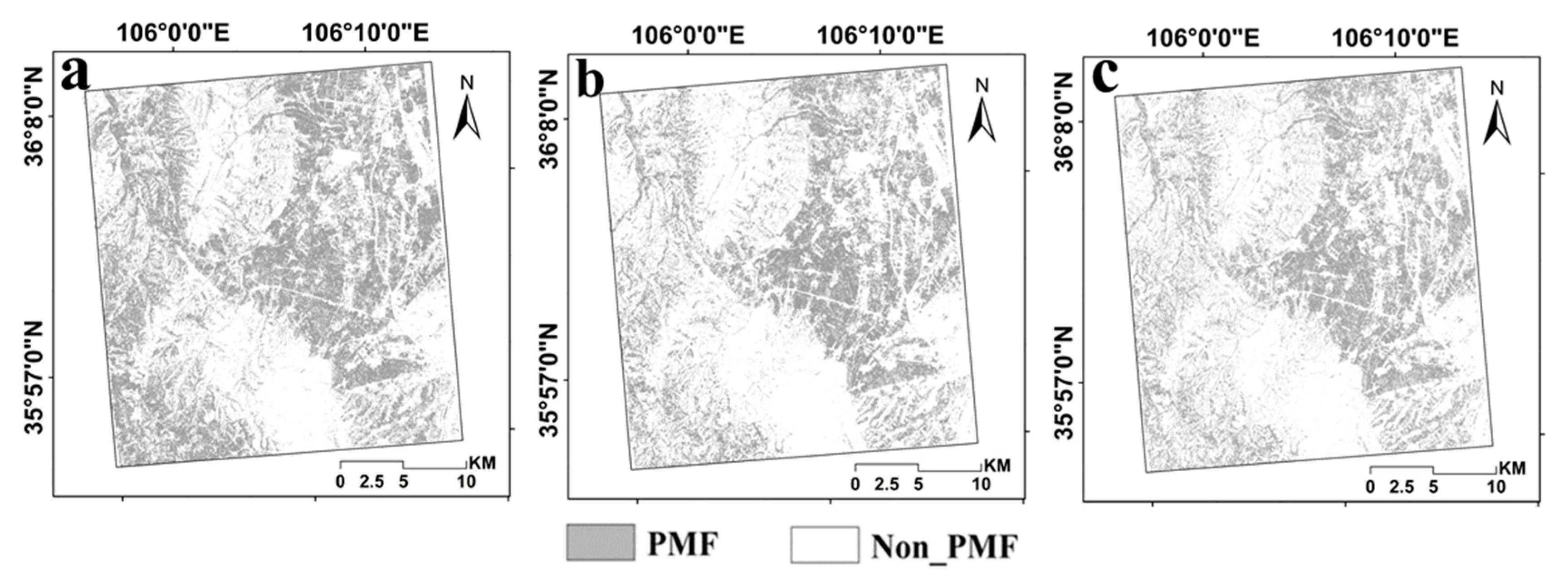
Figure 8 and Figure 9 show the spatial distribution of PMF in Jizhou and Guyuan obtained from RF and SVM using Radarsat-2 data, respectively. The general spatial pattern is consistent with the knowledge obtained from the field survey. However, there is some visible classification noise that can be ascribed to speckle noise, carrying serious omission and commission error, of SAR data. Compared with the classification results from SVM, the misclassification of the RF classifier is less.
5. Discussion
The highest classification accuracy of PMF obtained from the Radarsat-2 data is close to 75%. However, it is relatively lower than the results from optical remote sensing data [27,28,29]. The reasons can be attributed to the data type, the data processing, the characteristics of the classified land cover types and the other factors.
5.1. The Data and Features
In terms of data type, Radarsat-2 data are obtained from a C-band (long-wave radar system) radar system. Compared with the X-, L- and S-bands (short-wave radar system), C-band has a certain ability to penetrate the thin surface (such as the canopy) to monitor the soil surface below the vegetation. Therefore, there was serious confusion between vegetation and bare soil, vegetation and PMF to a certain degree. In terms of the data processing, the features used in this study include backscattering intensity of the four modes of polarization (HH, VV, VH and HV) and a number of polarimetric decomposition descriptors. Therefore, the parameters used in the data preprocessing and the feature extraction process have some effect on the classification result, such as filtering window size, the parameters of polarization decomposition extraction, and so on. The impact of these factors should be discussed in further work. In addition, the land cover classification system of this study contains the land cover types with surface scattering, double-bounce scattering and volume scattering. Therefore, the inclusion of the polarization decomposition features leads to the improvement of the classification accuracy. However, PMF mainly reflects the surface scattering, which is very similar to the scattering characteristics of water body and bare soil. Thus, the PMF confused seriously with the water body and the bare soil in the classification process.
The accuracy improvement indicates that the polarimetric decomposition descriptors can provide valuable information for mapping PMF in these two study areas. Focusing on dominant scatter mechanisms, this research indicated that the surface scattering of H/A/Alpha polarimetric decompositions is the most important backscattering mechanism. The main contribution of the polarimetric decomposition descriptors extracted from Radarsat-2 images is to alleviate the confusion between PMF and water body (7.97%), between PMF and vegetation cover (11.73%) and between PMF and impervious surface (5.23%) in Jizhou. This can be attributed to the valuable information for mapping the impervious surface (built-up area) provided by the polarimetric decomposition descriptors. Although speckle filtering was used to the Radarsat-2 images, the speckle noise of SAR data still affected the classification accuracy significantly. Besides the speckle noise in backscattering intensity of different polarizations and coherency matrices, there was much noise, as well as in the polarimetric decomposition descriptors that were extracted later [42].
5.2. The Differences of Classifiers
Two pixel-based machine learning classifiers (RF and SVM) were used in this study to map PMF. There were some differences between the two classifiers. RF performed better than the SVM in most cases. We attribute this superiority to the combination of the flexibility of the tree-based techniques and the stability introduced by the bootstrap sampling. RF performed better than SVM, indicating the improved efficiency produced by integrating classifiers [67]. Therefore, RF is more effective in the high dimensional feature space and can avoid the problem of over-fitting. On the other hand, the performance of the classifier is related to the remote sensing data, the number of samples and the selected features.
In this section, we mainly discussed the influence of features selected by different algorithms (RF and SVM). We selected features using SVM feature selection algorithm and found that the order of important features was slightly different from that of RF feature selection (Table 9). Afterward, we mapped the PMF using RF based on the selected features from RF. Additionally, we also mapped the PMF using SVM based on the selected features from SVM. The results indicated that the classification accuracies of RF were higher than that of SVM when using the features selected by the same classifier (Table 10).
5.3. Difference in Regions
The difference of PMF classification accuracy between these two study areas can be attributed to the land cover types and their distribution pattern. The land cover types in Jizhou are simpler and distributed more uniformly (large plain agricultural land use), while the land cover types in Guyuan are more complex and distributed unevenly (Figure 10). In addition, the mulching mode in Guyuan includes mulching in autumn, mulching in early spring and mulching before sowing. The data used in this study were acquired in April. Therefore, there may be some discrepancies between the data acquisition time and the mulching time. As a result, the classification accuracy in Guyuan is lower than that in Jizhou.
5.4. Comparison with Previous Studies
Table 11 shows that a small number of research works have been conducted to map the PMF with remote sensing data. All the existing studies have only used optical remote sensing data. SAR remote sensing data have never been used to map PMF until now. Definitely, the classification accuracy obtained from optical remote sensing data is much higher than that generated from SAR remote sensing data. However, SAR remote sensing data have their unique advantages over optical remote sensing data for mapping land cover types. It is well known that the SAR can provide all-weather and all-day data, which can fill the data missing due to cloudy weather or nighttime. Therefore, for the agricultural remote sensing operational monitoring system, SAR remote sensing data can be considered as powerful supplemental and alternative data for optical remote sensing data. In addition, SAR data can provide the structural information for mapping, which is hard to provide from optical remote sensing data. Therefore, the SAR data can be an important compensation for optical remote sensing in land cover classification. However, the relatively lower classification accuracy of SAR data can be attributed to the speckle noise (the inherent shortcomings of SAR data) and the confusion with other land cover types. This problem can also be resolved by using optical remote sensing data to mask the special land cover types (the water body or the bare soil), which were easily confused with PMF on the SAR image.
6. Conclusions
The consideration of SAR data makes a novel contribution to map PMF in northern China. Our preliminary conclusions are as follows:
The space-borne full-polarimetric C-band Radarsat-2 data are found to be applicable for mapping PMF in northern China generally. The highest accuracy is 74.82% in Jizhou and 64.21% in Guyuan, respectively.
The analysis of feature importance by RF indicated that the polarimetric decomposition features are more important than the backscattering intensity of four polarizations. The results also suggested that the descriptors from H/A/Alpha decomposition are more important than the descriptors from other polarimetric decompositions for PMF mapping. The inclusion of polarimetric decomposition descriptors is found to improve the classification accuracy considerably.
In terms of classifiers, RF performed significantly better than SVM with regards to PMF classification accuracy and efficiency.
This study indicates that promising results can be achieved for mapping PMF in northern China by using full-polarization C-band Radarsat-2 and machine learning algorithms. Further researches should focus on the following aspects: (1) we will assess the effectiveness of X-band SAR data for mapping PMF; (2) we will transfer this presented methodology to the south region of China, which is affected seriously by cloudy and rainy weather; (3) we will introduce the object-oriented algorithm to relieve the inherent speckle noise effect of SAR data themselves; (4) and we will improve the classification accuracy by combining SAR remote sensing data and optical remote sensing data.
Acknowledgments
This work was jointly supported by the National Natural Science Foundation of China (Grant No. NSFC-61661136006), China Ministry of Agriculture “Introduction of International Advanced Agricultural Science and Technology Program (948 Program)” project (No. 2016-X38) and the Open Fund of the Ministry of Agriculture National Outstanding Researcher Fund and the Key Laboratory of Agricultural Remote Sensing, Ministry of Agriculture, China (No. 2016003).
Author Contributions
Hasituya designed and conducted the experiments and wrote the manuscript. Zhongxin Chen provided suggestions for the data analysis and manuscript writing. Fei Li and Hongmei provided suggestions for manuscript writing.
Conflicts of Interest
The authors declare no conflict of interest.
References
- Bai, L.; Hai, J.; Han, Q.; Jia, Z. Effects of mulching with different kinds of plastic film on growth and water use efficiency of winter wheat in Weibei Highland. Agric. Res. Arid Areas 2010, 28, 135–139. [Google Scholar]
- Yan, C.; Mei, X.; He, W.; Zheng, S. Present situation of residue pollution of mulching plastic film and controlling measures. Trans. Chin. Soc. Agric. Eng. 2006, 22, 269–272. [Google Scholar]
- Zhang, D. Study on collection of used plastic film in fields. J. China Agric. Univ. 1998, 3, 103–106. [Google Scholar]
- Lu, L.; Di, L.; Ye, Y. A Decision-Tree Classifier for Extracting Transparent Plastic-Mulched Landcover from Landsat-5 TM Images. IEEE J.-STARS 2014, 7, 4548–4558. [Google Scholar] [CrossRef]
- Yan, C.; Liu, E.; Shu, F.; Liu, Q.; Liu, S.; He, W. Review of agricultural plastic mulching and its residual pollution and prevention measures in China. J. Agric. Resour. Environ. 2014, 31, 95–102. [Google Scholar]
- Nordberg, M.L.; Evertson, J. Monitoring change in mountainous dry-heath vegetation at a regional scale using multitemporal Landsat TM data. AMBIO 2003, 32, 502–509. [Google Scholar] [CrossRef] [PubMed]
- Subramaniam, S.; Babu, A.V.S.; Roy, P.S. Automated Water Spread Mapping Using ResourceSat-1 AWiFS Data for Water Bodies Information System. IEEE J.-STARS 2011, 4, 205–215. [Google Scholar] [CrossRef]
- Zhou, Y.; Luo, J.; Shen, Z.; Hu, X.; Yang, H. Multiscale Water Body Extraction in Urban Environments from Satellite Images. IEEE J.-STARS 2014, 7, 4301–4312. [Google Scholar] [CrossRef]
- Zhang, Y.; Zhang, H.; Lin, H. Improving the impervious surface estimation with combined use of optical and SAR remote sensing images. Remote Sens. Environ. 2014, 141, 155–167. [Google Scholar] [CrossRef]
- Makynen, M.; Simila, M. Thin Ice Detection in the Barents and Kara Seas With AMSR-E and SSMIS Radiometer Data. IEEE Trans. Geosci. Remote Sens. 2015, 53, 5036–5053. [Google Scholar] [CrossRef]
- Thompson, J.A.; Paull, D.J.; Lees, B.G. Using phase-spaces to characterize land surface phenology in a seasonally snow-covered landscape. Remote Sens. Environ. 2015, 166, 178–190. [Google Scholar] [CrossRef]
- Nijland, W.; Addink, E.A.; De Jong, S.M.; Van der Meer, F.D. Optimizing spatial image support for quantitative mapping of natural vegetation. Remote Sens. Environ. 2009, 113, 771–780. [Google Scholar] [CrossRef]
- Agüera, F.; Aguilar, M.A.; Aguilar, F.J. Detecting greenhouse changes from QuickBird imagery on the Mediterranean coast. Int. J. Remote Sens. 2006, 27, 4751–4767. [Google Scholar] [CrossRef]
- Agüera, F.; Liu, J.G. Automatic greenhouse delineation from QuickBird and Ikonos satellite images. Comput. Electron. Agric. 2009, 66, 191–200. [Google Scholar] [CrossRef]
- Carvajal, F.; Agüera, F.; Aguilar, F.J.; Aguilar, M.A. Relationship between atmospheric corrections and training-site strategy with respect to accuracy of greenhouse detection process from very high resolution imagery. Int. J. Remote Sens. 2010, 31, 2977–2994. [Google Scholar] [CrossRef]
- Arcidiacono, C.; Porto, S.M.C. A model to manage crop-shelter spatial development by multi-temporal coverage analysis and spatial indicators. Biosyst. Eng. 2010, 107, 107–122. [Google Scholar] [CrossRef]
- Arcidiacono, C.; Porto, S.M.C.; Cascone, G. Accuracy of crop-shelter thematic maps: A case study of maps obtained by spectral and textural classification of high-resolution satellite images. J. Food Agric. Environ. 2012, 10, 1071–1074. [Google Scholar]
- Koc-San, D. Evaluation of different classification techniques for the detection of glass and plastic greenhouses from WorldView-2 satellite imagery. J. Appl. Remote Sens. 2013, 7. [Google Scholar] [CrossRef]
- Aguilar, M.; Vallario, A.; Aguilar, F.; Lorca, A.; Parente, C. Object-Based Greenhouse Horticultural Crop Identification from Multi-Temporal Satellite Imagery: A Case Study in Almeria, Spain. Remote Sens. 2015, 7, 7378–7401. [Google Scholar] [CrossRef]
- Aguilar, M.; Bianconi, F.; Aguilar, F.; Fernández, I. Object-Based Greenhouse Classification from GeoEye-1 and WorldView-2 Stereo Imagery. Remote Sens. 2014, 6, 3554–3582. [Google Scholar] [CrossRef]
- Aguilar, M.; Nemmaoui, A.; Novelli, A.; Aguilar, F.; García Lorca, A. Object-Based Greenhouse Mapping Using Very High Resolution Satellite Data and Landsat 8 Time Series. Remote Sens. 2016, 8, 513. [Google Scholar] [CrossRef]
- Novelli, A.; Aguilar, M.A.; Nemmaoui, A.; Aguilar, F.J.; Tarantino, E. Performance evaluation of object based greenhouse detection from Sentinel-2 MSI and Landsat 8 OLI data: A case study from Almería (Spain). Int. J. Appl. Earth Obs. 2016, 52, 403–411. [Google Scholar] [CrossRef]
- Wu, C.F.; Deng, J.S.; Ke, W.; Ma, L.G.; Tahmassebi, A.R.S. Object-based classification approach for greenhouse mapping using Landsat-8 imagery. Int. J. Agric. Biol. Eng. 2016, 9, 79. [Google Scholar]
- Yang, D.D.; Chen, J.; Zhou, Y.; Chen, X.; Chen, X.; Cao, X. Mapping plastic greenhouse with medium spatial resolution satellite data: Development of a new spectral index. ISPRS J. Photogramm. 2017, 128, 47–60. [Google Scholar] [CrossRef]
- Levin, N.; Lugass, R.; Ramon, U.; Braun, O.; Ben-Dor, E. Remote sensing as a tool for monitoring plasticulture in agricultural landscapes. Int. J. Remote Sens. 2007, 28, 183–202. [Google Scholar] [CrossRef]
- Lu, L.; Hang, D.; Di, L. Threshold model for detecting transparent plastic-mulched landcover using moderate-resolution imaging spectroradiometer time series data: A case study in southern Xinjiang, China. J. Appl. Remote Sens. 2015, 9. [Google Scholar] [CrossRef]
- Hasituya; Chen, Z.X.; Wang, L.M.; Wu, W.B.; Jiang, Z.W.; Li, H. Monitoring Plastic-Mulched Farmland by Landsat-8 OLI Imagery Using Spectral and Textural Features. Remote Sens. 2016, 8, 353. [Google Scholar] [CrossRef]
- Hasituya; Chen, Z.X. Mapping Plastic-Mulched Farmland with Multi-Temporal Landsat-8 Data. Remote Sens. 2017, 9, 557. [Google Scholar] [CrossRef]
- Hasituya; Chen, Z.X.; Wang, L.M.; Liu, J. Selecting Appropriate Spatial Scale for Mapping Plastic-Mulched Farmland with Satellite Remote Sensing Imagery. Remote Sens. 2017. [Google Scholar] [CrossRef]
- Lanorte, A.; De Santis, F.; Nolè, G.; Blanco, I.; Loisi, R.V.; Schettini, E.; Vox, G. Agricultural plastic waste spatial estimation by Landsat 8 satellite images. Comput. Electron. Agric. 2017, 141, 35–45. [Google Scholar] [CrossRef]
- Yang, H.; Chen, E.; Li, Z.; Zhao, C.; Yang, G.; Pignatti, S.; Casa, R.; Zhao, L. Wheat lodging monitoring using polarimetric index from RADARSAT-2 data. Int. J. Appl. Earth Obs. 2015, 34, 157–166. [Google Scholar] [CrossRef]
- Maher, I.S.; Faten, H.N.; Faez, H.B.; Biswajeet, P.; Mohamed Shariff, A.R.B. A refined classification approach by integrating Landsat Operational Land Imager (OLI) and RADARSAT-2 imagery for land-use and land-cover mapping in a tropical area. Int. J. Remote Sens. 2016, 37, 2358–2375. [Google Scholar]
- Qi, Z.; Yeh, A.G.; Li, X.; Lin, Z. A novel algorithm for land use and land cover classification using RADARSAT-2 polarimetric SAR data. Remote Sens. Environ. 2012, 118, 21–39. [Google Scholar] [CrossRef]
- Heine, I.; Jagdhuber, T.; Itzerott, S. Classification and Monitoring of Reed Belts Using Dual-Polarimetric TerraSAR-X Time Series. Remote Sens. 2016, 8, 552. [Google Scholar] [CrossRef]
- Koppe, W.; Gnyp, M.L.; Huett, C.; Yao, Y.; Miao, Y.; Chen, X.; Bareth, G. Rice monitoring with multi-temporal and dual-polarimetric TerraSAR-X data. Int. J. Appl. Earth Obs. 2013, 21, 568–576. [Google Scholar] [CrossRef]
- Liu, C.; Shang, J.; Vachon, P.W.; McNairn, H. Multiyear Crop Monitoring Using Polarimetric Radarsat-2 Data. IEEE Trans. Geosci. Remote Sens. 2013, 51, 2227–2240. [Google Scholar] [CrossRef]
- Lopez-Sanchez, J.M.; Vicente-Guijalba, F.; Ballester-Berman, J.D.; Cloude, S.R. Polarimetric Response of Rice Fields at C-Band: Analysis and Phenology Retrieval. IEEE Trans. Geosci. Remote Sens. 2014, 52, 2977–2993. [Google Scholar] [CrossRef] [Green Version]
- Hajnsek, I.; Jagdhuber, T.; Schcoen, H.; Papathanassiou, K.P. Potential of Estimating Soil Moisture Under Vegetation Cover by Means of PolSAR. IEEE Trans. Geosci. Remote Sens. 2009, 47, 442–454. [Google Scholar] [CrossRef] [Green Version]
- Insom, P.; Cao, C.; Boonsrimuang, P.; Liu, D.; Saokarn, A.; Yomwan, P.; Xu, Y. A Support Vector Machine-Based Particle Filter Method for Improved Flooding Classification. IEEE Geosci. Remote Sens. Lett. 2015, 12, 1943–1947. [Google Scholar] [CrossRef]
- Liu, C.; Yin, J.; Yang, J. Coastline detection in polarimetric SAR images based on mixed edge detection. Syst. Eng. Electron. 2016, 38, 1262–1267. [Google Scholar]
- Nunziata, F.; Buono, A.; Migliaccio, M.; Benassai, G. Dual-Polarimetric C- and X-Band SAR Data for Coastline Extraction. IEEE J.-STARS 2016, 9, 4921–4928. [Google Scholar] [CrossRef]
- Zhang, G.; Perrie, W.; Li, X.; Zhang, J.A. A Hurricane Morphology and Sea Surface Wind Vector Estimation Model Based on C-Band Cross-Polarization SAR Imagery. IEEE Trans. Geosci. Remote Sens. 2017, 55, 1743–1751. [Google Scholar] [CrossRef]
- Ivonin, D.V.; Skrunes, S.; Brekke, C.; Ivanov, A.Y. 1 Interpreting sea surface slicks on the basis of the normalized radar cross-section model using RADARSAT-2 copolarization dual-channel SAR images. Geophys. Res. Lett. 2016, 43, 2748–2757. [Google Scholar] [CrossRef]
- You, B. Analysis and Application of Target’s Scattering Property in Polarimetric SAR Images. Ph.D. Thesis, Tsinghua University, Beijing, China, 2014. [Google Scholar]
- Shang, B. Quality Inspection and Quality Analysis of Hebei Province Jizhou City Environment. Master’s Thesis, Northwest Agriculture & Forestry University, Xianyang, China, 2014. [Google Scholar]
- Huang, X.; Wang, J.; Shang, J.; Liao, C.; Liu, J. Application of polarization signature to land cover scattering mechanism analysis and classification using multi-temporal C-band polarimetric RADARSAT-2 imagery. Remote Sens. Environ. 2017, 193, 11–28. [Google Scholar] [CrossRef]
- Moran, M.S.; Alonso, L.; Moreno, J.F.; Cendrero Mateo, M.P.; de la Cruz, D.F.; Montoro, A. A RADARSAT-2 Quad-Polarized Time Series for Monitoring Crop and Soil Conditions in Barrax, Spain. IEEE Trans. Geosci. Remote Sens. 2012, 50, 1057–1070. [Google Scholar] [CrossRef]
- European Space Agency PolSARpro. V. 4.2. Available online: http://earth.eo.esa.int/polsarpro/ (accessed on 1 November 2013).
- Wang, W.; Wang, J.; Mao, S.; Li, H. Ship detection based on classification of polarimetric SAR images. Signal Process. 2007, 23, 676–679. [Google Scholar]
- Van Beijma, S.; Comber, A.; Lamb, A. Random forest classification of salt marsh vegetation habitats using quad-polarimetric airborne SAR, elevation and optical RS data. Remote Sens. Environ. 2014, 149, 118–129. [Google Scholar] [CrossRef]
- You, B.; Yang, J.; Yin, J.; Xu, B. Decomposition of the Kennaugh Matrix Based on a New Norm. IEEE Geosci. Remote Sens. Lett. 2014, 11, 1000–1004. [Google Scholar] [CrossRef]
- Krogager, E.; Boerner, W.M.; Madsen, S.N. Feature-motivated Sinclair matrix (sphere/diplane/helix) decomposition and its application to target sorting for land feature classification. In Proceedings of the SPIE Conference on Wideband Interferometric Sensing and Imaging Polarimetry, San Diego, CA, USA, 23 December 1997; Volume 3120, pp. 144–154. [Google Scholar]
- Duguay, Y.; Bernier, M.; Lévesque, E.; Domine, F. Land Cover Classification in SubArctic Regions Using Fully Polarimetric Radarsat-2 Data. Remote Sens. 2016, 8, 697. [Google Scholar] [CrossRef]
- Yamaguchi, Y.; Moriyama, T.; Ishido, M.; Yamada, H. Four-component scattering model for polarimetric SAR image decomposition. IEEE Trans. Geosci. Remote Sens. 2005, 43, 1699–1706. [Google Scholar] [CrossRef]
- Gislason, P.O.; Benediktsson, J.A.; Sveinsson, J.R. Random Forests for land cover classification. Pattern Recognit. Lett. 2006, 27, 294–300. [Google Scholar] [CrossRef]
- Rodriguez-Galiano, V.F.; Chica-Olmo, M.; Abarca-Hernandez, F.; Atkinson, P.M.; Jeganathan, C. Random Forest classification of Mediterranean land cover using multi-seasonal imagery and multi-seasonal texture. Remote Sens. Environ. 2012, 121, 93–107. [Google Scholar] [CrossRef]
- Pal, M. Support vector machine-based feature selection for land cover classification: A case study with DAIS hyperspectral data. Int. J. Remote Sens. 2006, 27, 2877–2894. [Google Scholar] [CrossRef]
- Duro, D.C.; Franklin, S.E.; Dube, M.G. A comparison of pixel-based and object-based image analysis with selected machine learning algorithms for the classification of agricultural landscapes using SPOT-5 HRG imagery. Remote Sens. Environ. 2012, 118, 259–272. [Google Scholar] [CrossRef]
- Heinzel, J.; Koch, B. Investigating multiple data sources for tree species classification in temperate forest and use for single tree delineation. Int. J. Appl. Earth Obs. 2012, 18, 101–110. [Google Scholar] [CrossRef]
- Yousefi, S.; Tazeh, M.; Mirzaee, S.; Moradi, H.R.; Tavangar, S.H. Comparison of different classification algorithms in satellite imagery to produce land use maps (Case study: Noor city). J. Appl. RS GIS Tech. Nat. Resour. Sci. 2011, 2, 15–25. [Google Scholar]
- Feng, Q.; Zhou, L.; Chen, E.; Liang, X.; Zhao, L.; Zhou, Y. The Performance of Airborne C-Band PolInSAR Data on Forest Growth Stage Types Classification. Remote Sens. 2017, 9, 955. [Google Scholar] [CrossRef]
- Waske, B.; van der Linden, S.; Benediktsson, J.A.; Rabe, A.; Hostert, P. Sensitivity of Support Vector Machines to Random Feature Selection in Classification of Hyperspectral Data. IEEE Trans. Geosci. Remote Sens. 2010, 48, 2880–2889. [Google Scholar] [CrossRef]
- Chen, Y.; Zhao, X.; Lin, Z. Optimizing Subspace SVM Ensemble for Hyperspectral Imagery Classification. IEEE J.-STARS 2014, 7, 1295–1305. [Google Scholar] [CrossRef]
- Congalton, R.G.; Green, K. Assessing the Accuracy of Remotely Sensed Data: Principles and Practices, 2nd ed.; Taylor & Francis Group: New York, NY, USA, 2009. [Google Scholar]
- KopeĿ, D.; Michalska-Hejduk, D.; Sſawik, S.; Berezowski, T.; Borowski, M.; Rosadziſski, S.; Chormaſski, J. Application of multisensoral remote sensing data in the mapping of alkaline fens Natura 2000 habitat. Ecol. Indic. 2016, 70, 196–208. [Google Scholar] [CrossRef]
- Guan, H.; Li, J.; Chapman, M.; Deng, F.; Ji, Z.; Yang, X. Integration of orthoimagery and lidar data for object-based urban thematic mapping using random forests. Int. J. Remote Sens. 2013, 34, 5166–5186. [Google Scholar] [CrossRef]
- Xu, L.; Li, J.; Brenning, A. A comparative study of different classification techniques for marine oil spill identification using RADARSAT-1 imagery. Remote Sens. Environ. 2014, 141, 14–23. [Google Scholar] [CrossRef]
Figure 1.
The location of the study areas ((a) is the location of the study area in Guyuan; and (b) is the location of the study area in Jizhou).
Figure 1.
The location of the study areas ((a) is the location of the study area in Guyuan; and (b) is the location of the study area in Jizhou).
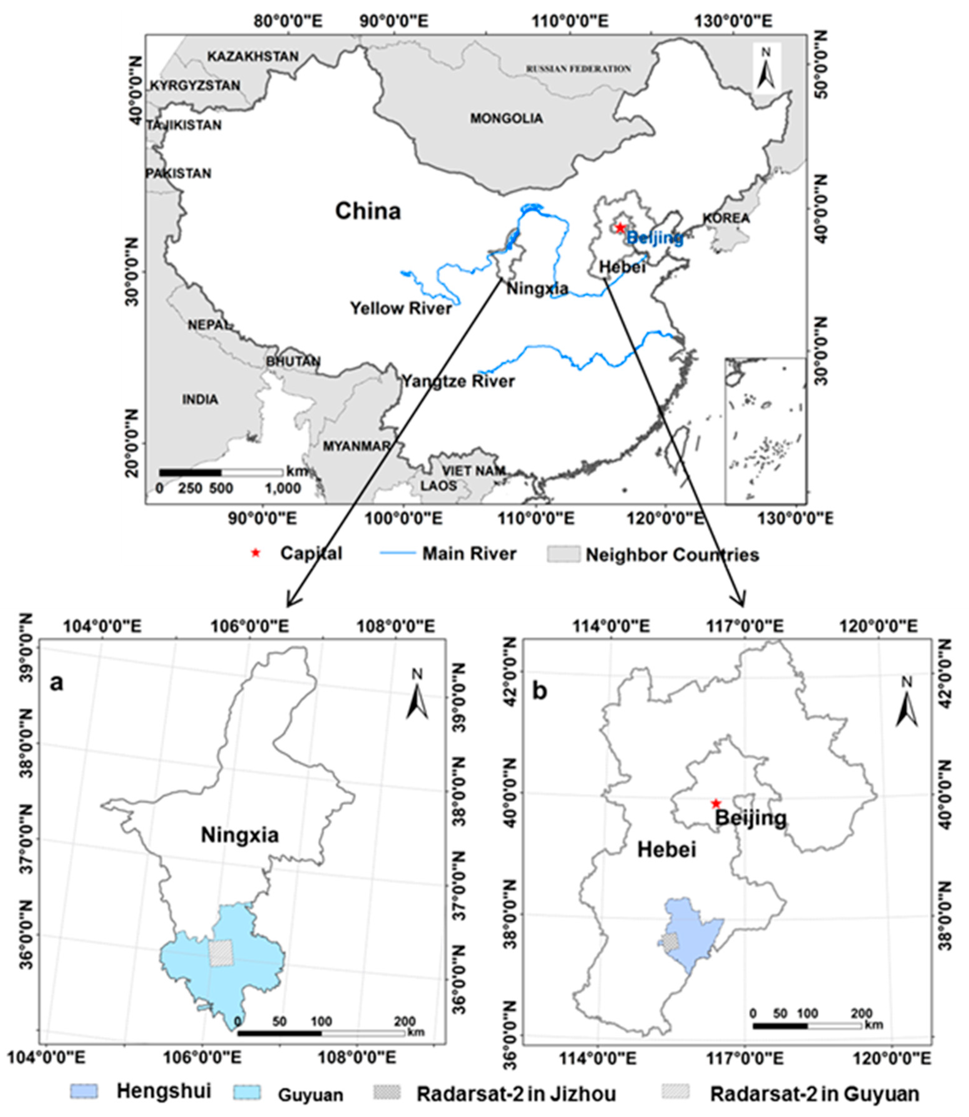
Figure 2.
The distribution of collected samples: (a) samples of land cover types in Guyuan; (b) samples of land cover types in Jizhou; two scenes of GF-1 images are displayed in false color composition (R: NIR, G: red, B: green).
Figure 2.
The distribution of collected samples: (a) samples of land cover types in Guyuan; (b) samples of land cover types in Jizhou; two scenes of GF-1 images are displayed in false color composition (R: NIR, G: red, B: green).

Figure 3.
Workflow of this study (H denotes Entropy from H/A/Alpha decomposition and A denotes Anisotropy from H/A/Alpha decomposition).
Figure 3.
Workflow of this study (H denotes Entropy from H/A/Alpha decomposition and A denotes Anisotropy from H/A/Alpha decomposition).

Figure 4.
The backscattering intensity of land cover types on Radarsat-2 images in Jizhou.
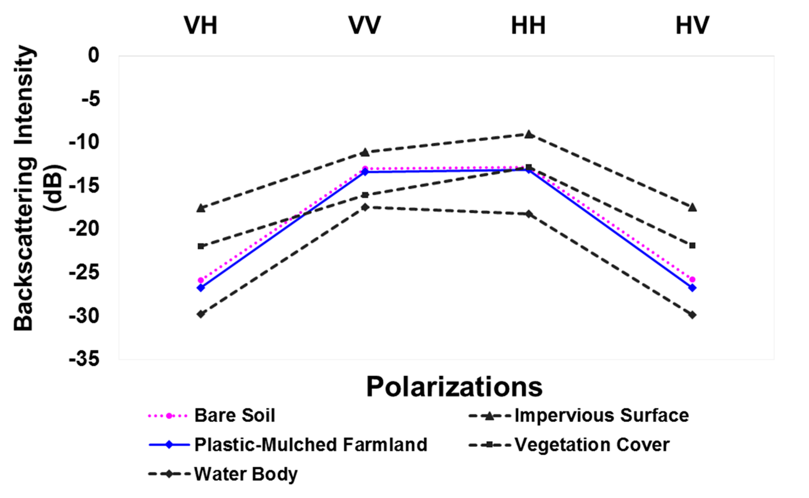
Figure 5.
The backscattering intensity of land cover types on Radarsat-2 images in Guyuan.

Figure 6.
Bar graph (including the standard deviation) showing the SAR features’ importance assessed by RF for mapping PMF in Jizhou and Guyuan.
Figure 6.
Bar graph (including the standard deviation) showing the SAR features’ importance assessed by RF for mapping PMF in Jizhou and Guyuan.
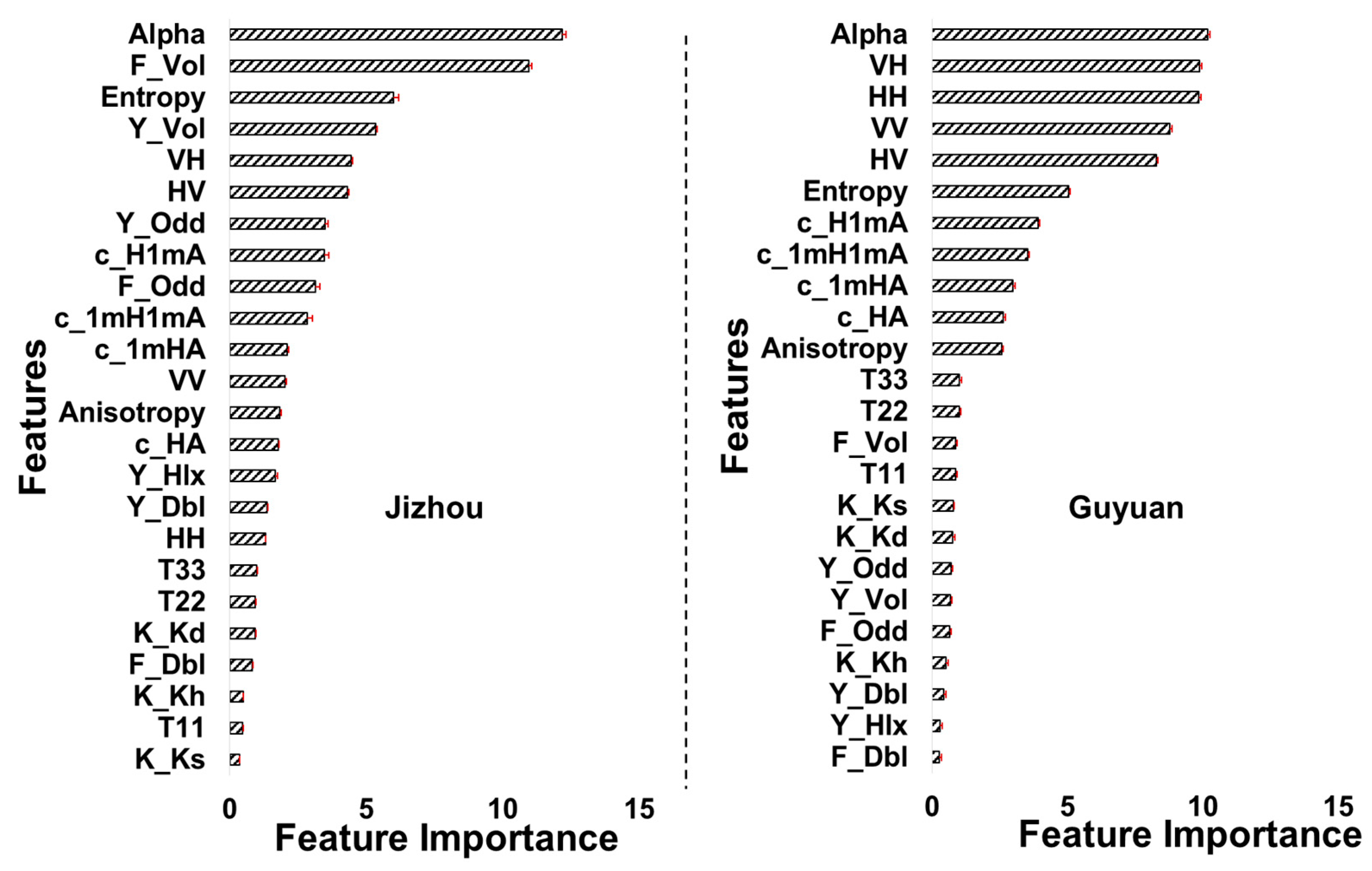
Figure 7.
The images of H/A/Alpha polarization decomposition (the red dashed rectangle represents the main PMF region).
Figure 7.
The images of H/A/Alpha polarization decomposition (the red dashed rectangle represents the main PMF region).
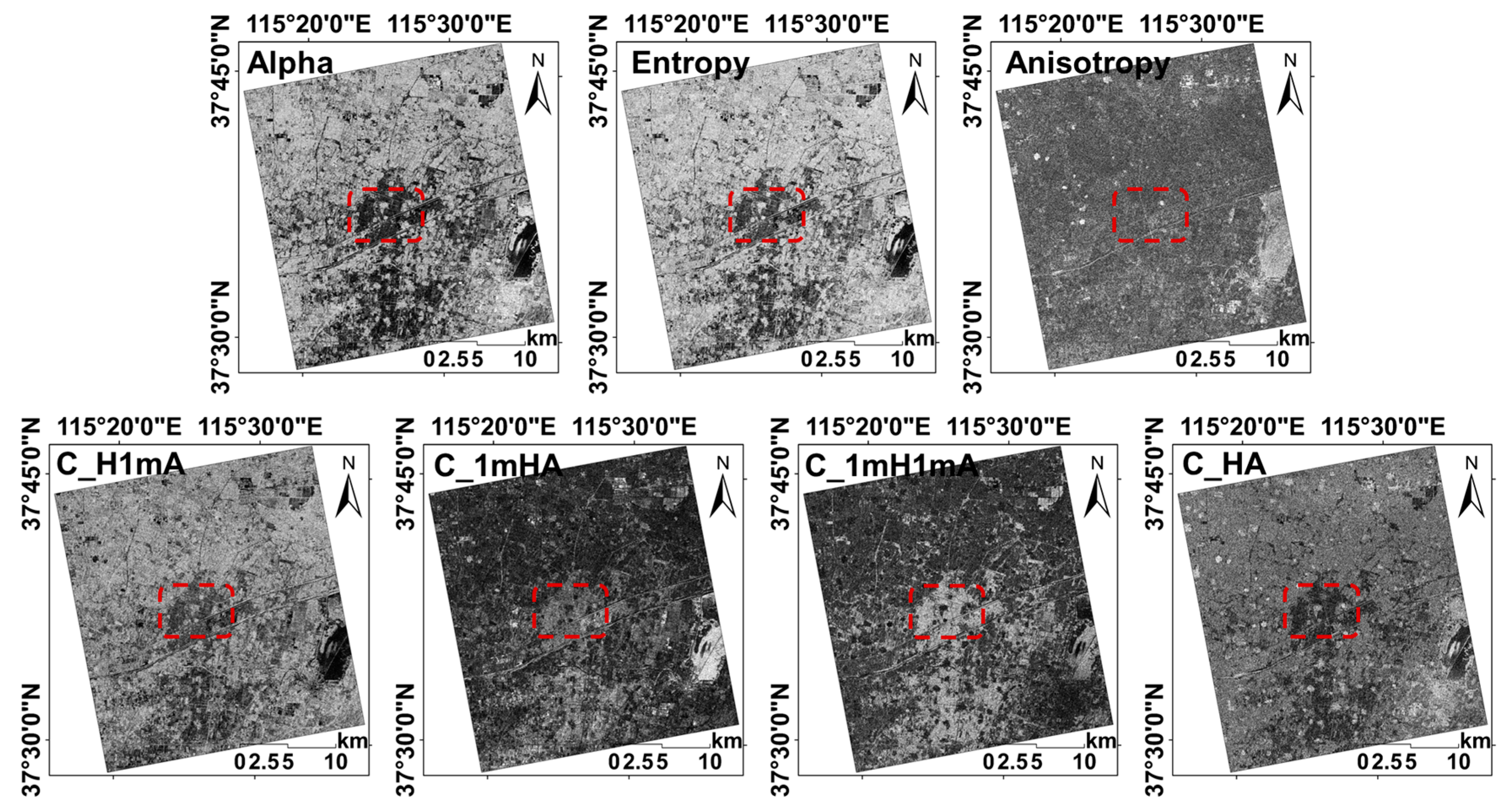
Figure 8.
The spatial distribution of PMF in Jizhou ((a) result from RF using backscattering intensity of four polarizations, (b) result from RF using all features, (c) result from SVM using all features).
Figure 8.
The spatial distribution of PMF in Jizhou ((a) result from RF using backscattering intensity of four polarizations, (b) result from RF using all features, (c) result from SVM using all features).
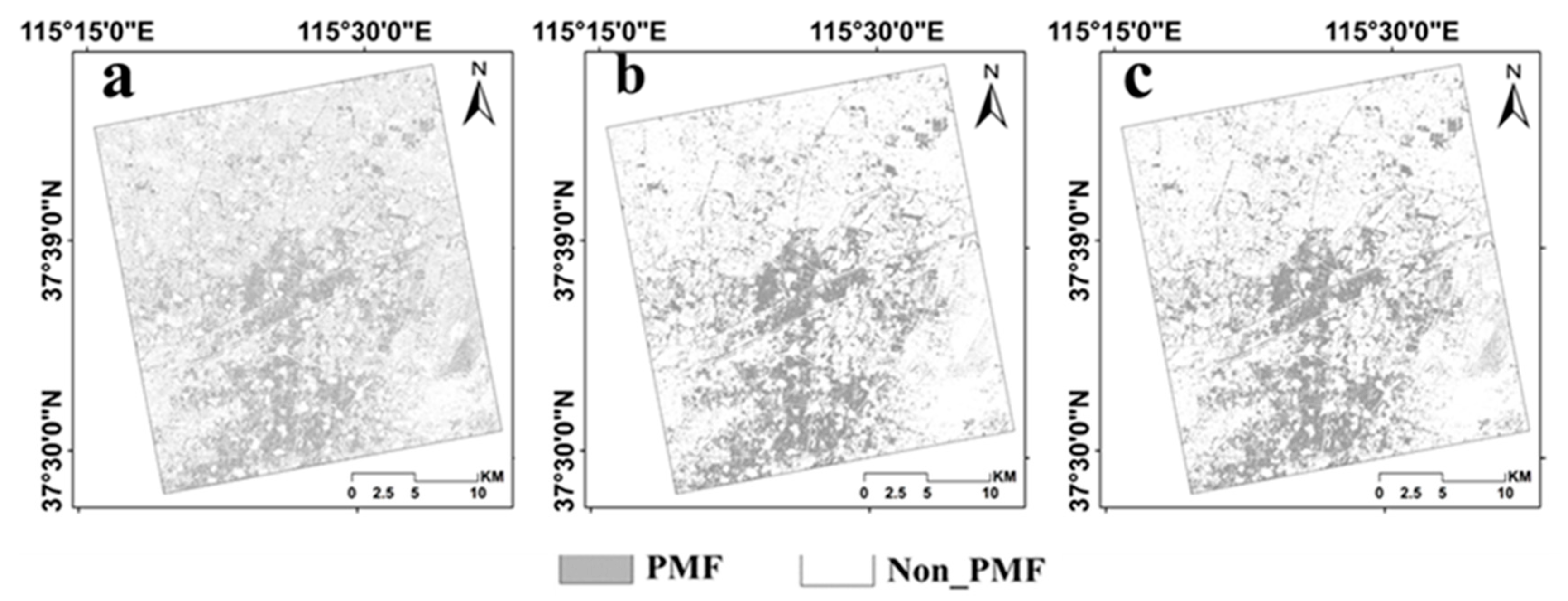
Figure 9.
The spatial distribution of PMF in Guyuan ((a) result from RF using backscattering intensity of four polarizations, (b) result from RF using all features, (c) result from SVM using all features).
Figure 9.
The spatial distribution of PMF in Guyuan ((a) result from RF using backscattering intensity of four polarizations, (b) result from RF using all features, (c) result from SVM using all features).

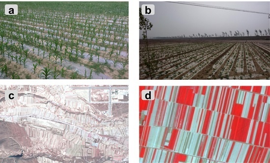
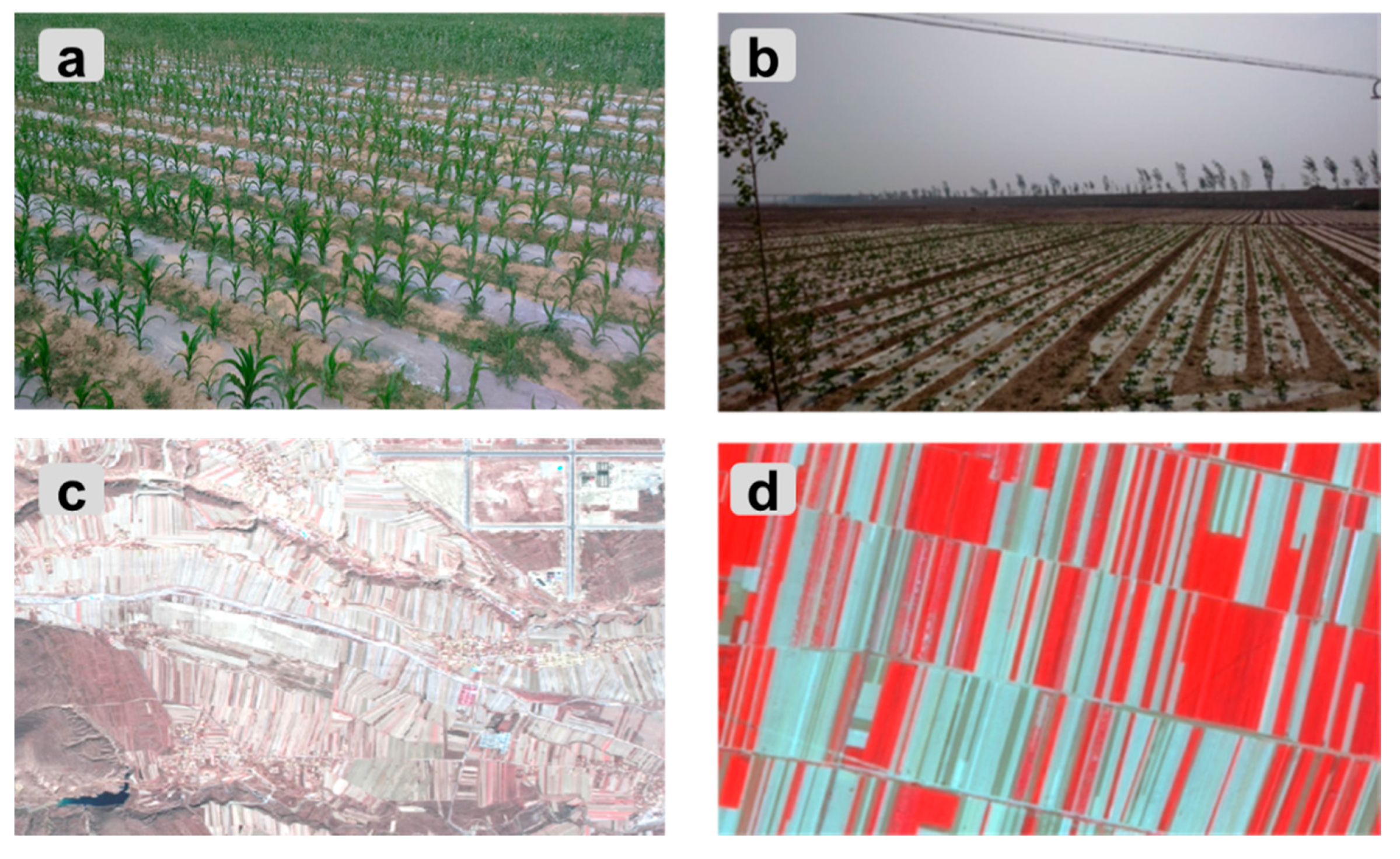
Figure 10.
The photo and GF-1 image showing PMF in Jizhou and Guyuan: (a) field photo of PMF in Guyuan; (b) field photo of PMF in Jizhou; (c) GF-1 image of PMF in Guyuan; (d) GF-1 image of PMF in Jizhou; two GF-1 images are displayed in false color composite (R: NIR, G: red, B: green).
Figure 10.
The photo and GF-1 image showing PMF in Jizhou and Guyuan: (a) field photo of PMF in Guyuan; (b) field photo of PMF in Jizhou; (c) GF-1 image of PMF in Guyuan; (d) GF-1 image of PMF in Jizhou; two GF-1 images are displayed in false color composite (R: NIR, G: red, B: green).

Table 1.
Parameters of Radarsat-2 satellite data in Jizhou and Guyuan
| Parameters of Radarsat-2 | Jizhou | Guyuan |
|---|---|---|
| Nominal swatch width | 25 km | 25 km |
| Wavelength/frequency | C-band (5.405 GHz, 5.54 cm) | C-band (5.405 GHz, 5.54 cm) |
| Polarization | Full quad-polarization HH + VV + HV + VH | Full quad-polarization HH + VV + HV + VH |
| Resolution of range | 4.73 m | 9.14 m |
| Resolution of azimuth | 4.74 m | 5.18 m |
| Incidence angle | 25.91° | 30.42° |
| Repeated cycle | 24 days | 24 days |
| Acquired date | 25 April 2015 | 27 April 2015 |
| Image center | 37°37′N/115°27′E | 36°03′N/106°07′E |
| Upper left corner | 37°43′N/115°18′E | 36°09′N/105°58′E |
| Upper right corner | 37°29′N/115°21′E | 35°54′N/106°01′E |
| Lower left corner | 37°46′N/115°34′E | 36°11′N/106°13′E |
| Lower right corner | 37°32′N/115°37′E | 35°57′N/106°17′E |
Table 2.
The land cover classification scheme and the number of collected samples in Jizhou and Guyuan.
Table 2.
The land cover classification scheme and the number of collected samples in Jizhou and Guyuan.
| Land Cover Types | Remarks | Number of Samples | |
|---|---|---|---|
| Jizhou | Guyuan | ||
| Plastic-Mulched Farmland (PMF) | White Plastic Film | 189 | 161 |
| Impervious Surface (IS) | Buildings, Factories, Road, and Dam Boundaries | 165 | 139 |
| Vegetation Cover (VC) | Crop, Vegetable Field, Grassland, Woodland | 197 | 101 |
| Water Body (WB) | Rivers, Lakes and Irrigation Canals | 64 | 30 |
| Bare Soil (BS) | Bare Land, Fallow land and Abandoned Land | 93 | 71 |
| Plastic Greenhouse (PG) | Walk-in or Medium Plastic Tunnel | - | 30 |
| Mountain Area (MA) | Mountain Area | - | 121 |
| Sum of Samples | - | 708 | 653 |
Table 3.
The polarimetric decomposition descriptors extracted from Radarsat-2 image.
| Polarimetric Decomposition Methods | Polarimetric Decomposition Descriptors | Abbreviation |
|---|---|---|
| Yamaguchi4 | Yamaguchi4_Dbl | Y_Dbl |
| Yamaguchi4_Hlx | Y_Hlx | |
| Yamaguchi4_Odd | Y_Odd | |
| Yamaguchi4_Vol | Y_Vol | |
| Freeman | Freeman_Dbl | F_Dbl |
| Freeman_Odd | F_Odd | |
| Freeman_Vol | F_Vol | |
| H/A/Alpha | Alpha | Alpha |
| Anisotropy | Anisotropy | |
| Entropy | Entropy_ | |
| Combination_1mH1mA | C_1mH1mA | |
| Combination_1mHA | C_1mHA | |
| Combination_H1mA | C_H1mA | |
| Combination_HA | C_HA | |
| Krogager | Krogager_Ks | K_Ks |
| Krogager_Kh | K_Kh | |
| Krogager_Kd | K_Kd |
Table 4.
The classification accuracy of PMF using Radarsat-2 data.
| Classifiers | Features | Jizhou | Guyuan | ||||||
|---|---|---|---|---|---|---|---|---|---|
| OA | CI of OA | PA | UA | OA | CI of OA | PA | UA | ||
| RF | 100% | 74.82 | 74.00–75.64 | 85.31 | 66.73 | 64.21 | 63.67–64.75 | 74.49 | 51.93 |
| 90% | 73.81 | 72.98–74.64 | 80.73 | 67.56 | 63.49 | 62.95–64.03 | 72.80 | 51.88 | |
| 80% | 73.36 | 72.53–74.19 | 79.82 | 67.46 | 63.26 | 62.72–63.80 | 72.29 | 52.14 | |
| Backscattering Intensity | 59.75 | 58.83–60.67 | 68.29 | 52.71 | 56.83 | 55.28–57.38 | 65.43 | 49.69 | |
| SVM | 100% | 73.45 | 72.62– 74.28 | 84.51 | 66.44 | 63.97 | 63.43–64.51 | 70.85 | 51.13 |
| 90% | 73.06 | 72.22– 73.90 | 81.99 | 65.84 | 62.81 | 62.27–63.35 | 69.57 | 50.92 | |
| 80% | 73.14 | 72.30– 73.98 | 78.79 | 67.24 | 62.11 | 61.57–62.65 | 69.56 | 50.32 | |
| Backscattering Intensity | 58.25 | 57.32– 59.18 | 66.21 | 50.73 | 53.97 | 53.41–54.53 | 67.54 | 49.53 | |
Note: The highest accuracies from different features are highlighted in bold. OA denotes the Overall Accuracy. PA denotes the Producer’s Accuracy. UA denotes the User’s Accuracy and CI denotes the 95% confidence interval.
Table 5.
Z test values for testing the significance of mapping PMF in Jizhou and Guyuan.
| Classifiers | Features | Kappa | Z Statistic | p | ||
|---|---|---|---|---|---|---|
| Jizhou | Guyuan | Jizhou | Guyuan | |||
| RF | with the highest accuracy | 0.667 | 0.531 | 163.56 | 7.19 | <0.005 |
| with the worst accuracy | 0.469 | 0.439 | 101.38 | 16.95 | <0.005 | |
| SVM | with the highest accuracy | 0.649 | 0.649 | 156.25 | 6.84 | <0.005 |
| with the worst accuracy | 0.401 | 0.411 | 99.26 | 5.63 | <0.005 | |
Table 6.
Z test values for the pairwise comparison of the error matrices for mapping PMF in Jizhou and Guyuan.
Table 6.
Z test values for the pairwise comparison of the error matrices for mapping PMF in Jizhou and Guyuan.
| Pairwise Comparison | Z Statistic | p | |
|---|---|---|---|
| Jizhou | Guyuan | ||
| The highest accuracy of RF vs. The worst accuracy of RF | 32.13 | 19.32 | <0.005 |
| The highest accuracy of SVM vs. The worst accuracy of SVM | 29.83 | 17.56 | <0.005 |
| The highest accuracy of RF vs. The highest accuracy of SVM | 3.07 | 2.99 | <0.005 |
| The worst accuracy of RF vs. The worst accuracy of SVM | 28.99 | 16.83 | <0.005 |
Table 7.
The confusion matrix from RF in Jizhou.
| Features | OA: 59.75 | PA: 68.29 | UA: 52.71 | CI: 58.83–60.67 | |||
| Land Cover Types | WB | VC | PMF | BS | IS | Total | |
| Backscattering Intensity of four polarizations | WB | 560 | 52 | 157 | 91 | 7 | 867 |
| VC | 103 | 1985 | 379 | 246 | 500 | 3213 | |
| PMF | 267 | 454 | 1790 | 726 | 159 | 3396 | |
| BS | 44 | 77 | 214 | 100 | 54 | 489 | |
| IS | 54 | 561 | 81 | 131 | 2032 | 2859 | |
| Total | 1028 | 3129 | 2621 | 1294 | 2752 | 10,824 | |
| Optimized Feature Set | OA: 74.82 | PA: 85.31 | UA: 66.73 | CI: 74.00–75.64 | |||
| Land Cover Types | WB | VC | PMF | BS | IS | Total | |
| WB | 643 | 34 | 62 | 72 | 14 | 825 | |
| VC | 110 | 2587 | 145 | 224 | 211 | 3277 | |
| PMF | 181 | 88 | 2236 | 827 | 19 | 3351 | |
| BS | 28 | 72 | 165 | 146 | 21 | 432 | |
| IS | 66 | 348 | 13 | 25 | 2487 | 2939 | |
| Total | 1028 | 3129 | 2621 | 1294 | 2752 | 10,824 | |
Table 8.
The confusion matrix from RF in Guyuan.
| Features | OA: 56.83 | PA: 65.43 | UA: 49.69 | CI: 55.28–57.38 | |||||
| Land Cover Types | WB | VC | PMF | MA | PG | IS | BS | Total | |
| Backscattering Intensity of four polarizations | WB | 888 | 77 | 38 | 117 | 174 | 291 | 25 | 1610 |
| VC | 0 | 1057 | 447 | 1100 | 48 | 515 | 136 | 3303 | |
| PMF | 0 | 597 | 2968 | 861 | 16 | 78 | 1453 | 5973 | |
| MA | 0 | 1018 | 382 | 7192 | 386 | 1622 | 173 | 10,773 | |
| PG | 0 | 9 | 26 | 46 | 71 | 184 | 1 | 337 | |
| IS | 90 | 475 | 150 | 1130 | 609 | 5144 | 18 | 7616 | |
| BS | 0 | 209 | 525 | 202 | 7 | 20 | 128 | 1091 | |
| Total | 978 | 3442 | 4536 | 10,648 | 1311 | 7854 | 1934 | 30,703 | |
| Optimized Feature Set | OA: 64.21 | PA: 74.49 | UA: 51.93 | CI: 63.67–64.75 | |||||
| Land Cover Types | WB | VC | PMF | MA | PG | IS | BS | Total | |
| WB | 377 | 3 | 0 | 16 | 35 | 147 | 0 | 578 | |
| VC | 510 | 1637 | 306 | 658 | 30 | 441 | 83 | 3665 | |
| PMF | 0 | 639 | 3379 | 846 | 10 | 34 | 1599 | 6507 | |
| MA | 0 | 751 | 320 | 8143 | 185 | 1064 | 142 | 10,605 | |
| PG | 0 | 6 | 0 | 6 | 84 | 168 | 4 | 268 | |
| IS | 90 | 355 | 136 | 847 | 967 | 5999 | 10 | 8404 | |
| BS | 1 | 51 | 395 | 132 | 0 | 1 | 96 | 676 | |
| Total | 978 | 3442 | 4536 | 10,648 | 1311 | 7854 | 1934 | 30,703 | |
Table 9.
The order of the features selected by RF and SVM in two study areas.
| No. | Order of Features | |||
|---|---|---|---|---|
| Jizhou | Guyuan | |||
| RF | SVM | RF | SVM | |
| 1 | Alpha | VH | Alpha | HV |
| 2 | F_Vol | F_Vol | VH | VH |
| 3 | Entropy | HH | HH | Alpha |
| 4 | Y_Vol | Anisotropy | VV | Entropy |
| 5 | VH | VV | HV | C_H1mA |
| 6 | HH | Alpha | Entropy | F_Vol |
| 7 | Y_Odd | c_HA | C_H1mA | Anisotropy |
| 8 | c_H1mA | HV | C_1mH1mA | HH |
| 9 | F_Odd | Entropy | C_1mHA | VV |
| 10 | c_1mH1mA | c_H1mA | C_HA | C_1mHA |
| 11 | c_1mHA | Y_Hlx | Anisotropy | C_1mH1mA |
| 12 | VV | K_Ks | T22 | C_HA |
| 13 | Anisotropy | c_1mH1mA | T33 | Y_Vol |
| 14 | c_HA | F_Dbl | F_Vol | T22 |
| 15 | Y_Hlx | Y_Vol | T11 | T33 |
| 16 | Y_Dbl | T11 | K_Ks | F_Odd |
| 17 | HH | F_Odd | K_Kd | T11 |
| 18 | T33 | Y_Dbl | Y_Odd | Y_Odd |
| 19 | T22 | Y_Odd | Y_Vol | Y_Dbl |
| 20 | K_Kd | T22 | F_Odd | Y_Hlx |
| 21 | F_Dbl | T33 | K_Kh | Y_Odd |
| 22 | K_Kh | K_Kd | Y_Dbl | F_Dbl |
| 23 | T11 | c_1mHA | Y_Hlx | K_Kh |
| 24 | K_Ks | K_Kh | F_Dbl | K_Ks |
Table 10.
The overall classification accuracy of RF and SVM using the features selected by the same classifier (RF-RF denotes the accuracy of the RF classifier using the features selected by RF; SVM-SVM denotes the accuracy of the SVM classifier using the features selected by SVM).
Table 10.
The overall classification accuracy of RF and SVM using the features selected by the same classifier (RF-RF denotes the accuracy of the RF classifier using the features selected by RF; SVM-SVM denotes the accuracy of the SVM classifier using the features selected by SVM).
| Number of Features | Jizhou | Guyuan | ||
|---|---|---|---|---|
| RF-RF | SVM-SVM | RF-RF | SVM-SVM | |
| 24 | 74.82 | 73.14 | 64.21 | 63.57 |
| 15 | 73.81 | 74.02 | 63.49 | 63.04 |
| 10 | 73.36 | 72.52 | 63.26 | 62.53 |
Table 11.
Accuracies of the existing results.
| No. | OA | PA | UA | Data | Study Region | Reference |
|---|---|---|---|---|---|---|
| 1 | 92.84 | 99.70 | 94.58 | MODIS | Xinjiang, China | [26] |
| 2 | 97.82 | 100.0 | 95.90 | Landsat-5 | Xinjiang, China | [5] |
| 3 | 94.14 | 90.67 | 90.58 | Landsat-8 | Hebei, China | [27] |
| 4 | 97.01 | 92.48 | 96.40 | Landsat-8 | Hebei, China | [28] |
| 5 | 96.05 | 90.99 | 94.22 | GF-1 | Hebei, China | [29] |
| 6 | 74.82 | 85.31 | 66.73 | Radarsat-2 | Hebei, China | This study |
© 2017 by the authors. Licensee MDPI, Basel, Switzerland. This article is an open access article distributed under the terms and conditions of the Creative Commons Attribution (CC BY) license (http://creativecommons.org/licenses/by/4.0/).
Share and Cite
MDPI and ACS Style
Hasituya; Chen, Z.; Li, F.; Hongmei. Mapping Plastic-Mulched Farmland with C-Band Full Polarization SAR Remote Sensing Data. Remote Sens. 2017, 9, 1264. https://doi.org/10.3390/rs9121264
AMA Style
Hasituya, Chen Z, Li F, Hongmei. Mapping Plastic-Mulched Farmland with C-Band Full Polarization SAR Remote Sensing Data. Remote Sensing. 2017; 9(12):1264. https://doi.org/10.3390/rs9121264
Chicago/Turabian StyleHasituya, Zhongxin Chen, Fei Li, and Hongmei. 2017. "Mapping Plastic-Mulched Farmland with C-Band Full Polarization SAR Remote Sensing Data" Remote Sensing 9, no. 12: 1264. https://doi.org/10.3390/rs9121264
Note that from the first issue of 2016, this journal uses article numbers instead of page numbers. See further details here.